Embed Size (px)
Citation preview
Circular 1481
Field Observations During the Third Microwave Water and Energy Balance Experiment (MicroWEX-3): June
16 - December 21, 20041
Tzu-yun Lin, Jasmeet Judge, Kai-Jen Calvin Tien, Joaquin Casanova, Mi-young Jang, Orlando Lanni, Larry
Miller, and Fei Yan2
_______________________________________________________________________________________ 1. This document is Circular 1483, one of a series of the Agricultural and Biological Engineering Department, Florida Cooperative Extension
Service, Institute of Food and Agricultural Sciences, University of Florida. First published November 2005. Please visit the EDIS Web site at http://edis.ifas.ufl.edu.
2. Jasmeet Judge is an Assistant Professor and Director of Center for Remote Sensing (email: [email protected]); Joaquin Casanova is an Undergraduate Research Assistant; and Kai-Jen Tien, Mi-young Jang, and Fei Yan are Graduate Research Assistants. All authors are affiliated with the Agricultural and Biological Engineering Department, Institute of Food and Agricultural Sciences, University of Florida, Gainesville, 32611
The Institute of Food and Agricultural Sciences (IFAS) is an Equal Opportunity Institution authorized to provide research, educational information and other services only to individuals and institutions that function with non-discrimination with respect to race, creed, color, religion, age, disability, sex, sexual orientation, marital status, national origin, political opinions or affiliations. U.S. Department of Agriculture, Cooperative Extension Service, University of Florida, IFAS, Florida A. & M. University Cooperative Extension Program, and Boards of County Commissioners Cooperating. Larry Arrington, Dean.
Archival copy: for current recommendations see http://edis.ifas.ufl.edu or your local extension office.

i
TABLE OF CONTENTS
1. INTRODUCTION ……………………………………………………………………………… 1
2. OBJECTIVES ………………………………………………………………………………… 1
3. FIELD SETUP …………………………………………………………………………………… 1
4. SENSORS ………………………………………………………………………………………… 4
4.1 University of Florida C-band Microwave Radiometer (UFCMR) System ………… 4
4.1.1 Theory of operation …………………………………………………………… 5
4.2 Eddy Covariance System ………………………………………………………………… 7
4.3 Net Radiometer ………………………………………………………………………… 8
4.4 Thermal Infrared Sensor ………………………………………………………………… 9
4.5 Soil Moisture and Temperature Probes ………………………………………………… 9
4.6 Soil Heat Flux Plates……………………………………………………………………… 10
4.7 Rain gauges ……………………………………………………………………………… 10
4.8 Canopy temperatures …………………………………………………………………… 10
5. SOIL SAMPLING ……………………………………………………………………………… 10
5.1 Surface Roughness ……………………………………………………………………… 10
5.2 Gravimetric Soil Moisture ……………………………………………………………… 11
5.3 Soil Temperature and Moisture………………………………………………………………12
6. VEGETATION SAMPLING …………………………………………………………………… 12
6.1 Height and Width…………………………………………………………………………… 12
6.2 Leaf Area Index (LAI) ………………………………………………………………… 12
6.3 Green and Dry Biomass ………………………………………………………………… 12
6.4 Root Sampling …………………………………………………………………………… 12
6.5 Lint Yield ………………………………………………………………………………… 12
7. WELL SAMPLING ……………………………………………………………………………… 13
7.1 Groundwater sampling ………………………………………………………………… 13
7.2 Water level measurement ……………………………………………………………… 13
8. FIELD LOG …………………………………………………………………………………… 14
ACKNOWLEDGEMENT ………………………………………………………………………… 23
REFERENCES ………………………………………………………………………………… 23
A. FIELD OBSERVATIONS …………………………………………………………………… 24
i
Archival copy: for current recommendations see http://edis.ifas.ufl.edu or your local extension office.
1
1. INTRODUCTION
For accurate prediction of weather and near-term climate, root-zone soil moisture is one of the most crucial components driving the surface hydrological processes. Soil moisture in the top meter is also very important because it governs moisture and energy fluxes at the land-atmosphere interface and it plays a significant role in partitioning of the precipitation into runoff and infiltration. Energy and moisture fluxes at the land surface can be estimated by Soil-Vegetation-Atmosphere-Transfer (SVAT) models. These models are typically used in conjunction with climate prediction models and hydrological models. Even though the biophysics of moisture and energy transport is well-captured in most current SVAT models, the computational errors accumulate over time and the model estimates of soil moisture diverge from reality. One promising way to improve significantly model estimates of soil moisture is by assimilating remotely sensed data that is sensitive to soil moisture, for example microwave brightness temperatures, and updating the model state variables. The microwave brightness at low frequencies (< 10 GHz) is very sensitive to soil moisture in the top few centimeters in most vegetated surfaces. Many studies have been conducted in agricultural areas such as bare soil, grass, soybean, wheat, pasture, and corn to understand the relationship between soil moisture and microwave remote sensing. Most of these experiments conducted in agricultural regions have been short-term experiments that captured only a part of growing seasons. It is important to know how microwave brightness signature varies with soil moisture, evapotranspiration (ET), and biomass in a dynamic agricultural canopy with a significant biomass (4-6 kg/m2) throughout the growing season.
2. OBJECTIVES
The goal of MicroWEX-3 was to understand the land-atmosphere interactions during the growing season of cotton, and their effect on observed microwave brightness signatures at 6.7 GHz, matching that of the two satellite-based microwave radiometers (AMSR-E and AMSR). Specific objectives of MicroWEX-3 are:
1. To collect passive microwave and other ancillary data to develop and calibrate a dynamic microwave brightness model for cotton.
2. To collect energy and moisture flux data at land surface and in soil to develop and calibrate a dynamic SVAT model for cotton.
3. To evaluate feasibility of soil moisture retrievals using passive microwave data at 6.7 GHz for the growing cotton canopy.
4. To evaluate feasibility of using Mid Infrared Reflectance for estimating vegetation water content and biomass during the cotton growing season
3. FIELD SETUP
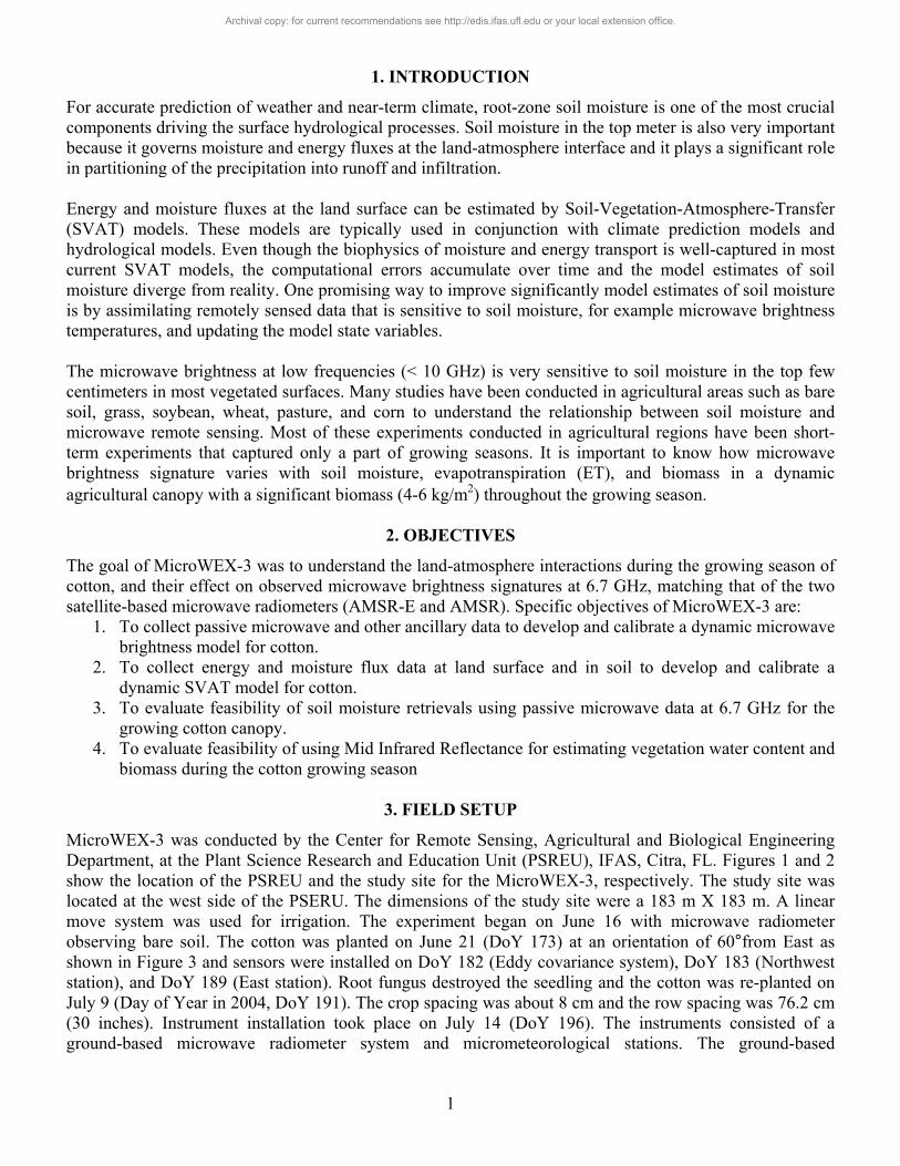
MicroWEX-3 was conducted by the Center for Remote Sensing, Agricultural and Biological Engineering Department, at the Plant Science Research and Education Unit (PSREU), IFAS, Citra, FL. Figures 1 and 2 show the location of the PSREU and the study site for the MicroWEX-3, respectively. The study site was located at the west side of the PSERU. The dimensions of the study site were a 183 m X 183 m. A linear move system was used for irrigation. The experiment began on June 16 with microwave radiometer observing bare soil. The cotton was planted on June 21 (DoY 173) at an orientation of 60°from East as shown in Figure 3 and sensors were installed on DoY 182 (Eddy covariance system), DoY 183 (Northwest station), and DoY 189 (East station). Root fungus destroyed the seedling and the cotton was re-planted on July 9 (Day of Year in 2004, DoY 191). The crop spacing was about 8 cm and the row spacing was 76.2 cm (30 inches). Instrument installation took place on July 14 (DoY 196). The instruments consisted of a ground-based microwave radiometer system and micrometeorological stations. The ground-based
Archival copy: for current recommendations see http://edis.ifas.ufl.edu or your local extension office.

2
microwave radiometer system was installed at the location shown in Figure 3, facing south to avoid the radiometer shadow interfering with the field of view as seen in Figure 3.
Figure 1. Location of PSREU/IFAS.
Figure 2. Location of the field site for MicroWEX-3 at the UF/IFAS PSREU.
MicroWEX-3 field site
Archival copy: for current recommendations see http://edis.ifas.ufl.edu or your local extension office.
3
The micrometeorological station was installed at the center of the field and included soil heat flux plates and the eddy covariance system. Two raingauges were installed at the east and west edge of the radiometer footprint. Two additional raingauges also were installed at the east and west edge of the field to capture the irrigation. Three stations with soil moisture, soil heat flux, and soil temperature sensors installed were set up at the location shown in Figure 3. The Northwest station was installed with a Thermal infrared camera and a net radiometer. This report provides detailed information regarding sensors deployed and data collected during the MicroWEX-3.
100 ft
: Wells
: CR23x, with soil moisture, soil temperature, and soil heat flux*
: CR10, with soil moisture, soil temperature, and soil heat flux*
:Footprint(12.5m*12.5m or 41ft*41ft) :Radiometer
N
18ft
(5.5m
)
600 ft (182.88m)
100ft(30.48m) 100ft(30.48m)100ft(30.48m)
100f
t(30.4
8m)
100f
t(30.4
8m)
200f
t (60
.96m
)20
0ft (
60.96
m)
200ft (60.96m)100ft(30.48m)
100f
t(30.4
8m)
: CR23x, with ECS
200f
t(60.9
6m)
*: The sensors are installed at depth: 2, 4, 8, 16, 32, 64, and 120 cm
Direction of
planting
X : Rainguages
XX
X X
60.6ft(18.5m)
:TIR :CNR
V.S.A. Vegetation: Sampling Area
V.S.A.
V.S.A. V.S.A.
V.S.A.
Figure 3. Layout of the sensors during MicroWEX-3.
Archival copy: for current recommendations see http://edis.ifas.ufl.edu or your local extension office.

4
4. SENSORS
MicroWEX-3 had three major types of instrument subsystems: the ground-based University of Florida C-band Radiometer (UFCMR), the micrometeorological subsystem, and the soil subsystem 4.1 University of Florida C-band Microwave Radiometer (UFCMR) System Microwave brightness temperatures at 6.7GHz (λ = 4.48 cm) were measured every 30 minutes using the University of Florida’s C-band Microwave Radiometer system (UFCMR) (Figure 4 (a)). The radiometer system consisted of a dual polarization total power radiometer operating at the center frequency of 6.7 GHz housed atop a 10 m tower installed on a 16’ trailer bed. UFCMR was designed and built by the Microwave Geophysics Group at the University of Michigan. It operates at the center frequency at 6.7 GHz that is identical to one of the center frequencies on the space borne Advanced Microwave Scanning Radiometer (AMSR) aboard the NASA Aqua Satellite Program. UFCMR observed a footprint of size 11 m X 11 m from a height of 7.6 m. A rotary system was used to rotate the look angle of the UFCMR both for field observations and sky measurements. The brightness temperatures were observed at an incidence angle of 55 degrees, matching that of the space borne AMSR-E sensor. The radiometer was calibrated every two weeks with a microwave absorber as warm load and measurements of sky at several angles as cold load. Figures 4 (b) and 4 (c) show the close-up of the rotary system and the antenna of the UFCMR, respectively. Table 1 lists the specifications of UFCMR. Figure A-1 shows the V- & H-pol brightness temperatures observed during MicroWEX-3.
Table 1. UFCMR specifications Parameter Qualifier Value Frequency Center 6.7 GHz Bandwidth 3 dB 20 MHz
3 dB V-pol elevation 23°a
3 dB V-pol azimuth 21°b 3 dB H-pol elevation 21°c
Beamwidth
3 dB H-pol azimuth 23°d Isolation > 27 dB Polarizations Sequential V/H Receiver temp 437 Ke Noise Figure From Trec 3.99 dB RF gain 85 dB Gain tempco dTsys/dTset -2 K/Cf
1 sec 0.71 Kg NEDT 8 sec 0.25 Kh
Tempature Control – rms 5 mKi Max 40° Cj SetPoint Min 0° C Max 48° Ck Ambient Min < 0° Cl
RF cutout McShane or RF1 thermistor 42° Cm Thermal shutdown Case thermistor 62° Cn
(a). sidelobes < -33 dB, (b). sidelobes < -28 dB, (c). sidelobes < -27 dB, (d). sidelobes < -35 dB, (e). +/- 20 K uncertainty, (f). looking at reference load, (g). tracking of absorber to reference load in lab, Tset = 305 K with PID = 0.75, 0.94, 0, (h). tracking of absorber to reference load in lab, Tset = 305 K with PID = 0.75, 0.94, 0, (i). Tset = 305 K in lab environment, on RF2, over 0.5 hour, after a day running, (j). active components rated to 65 C, filters to 40 C, (k). estimated absolute max Tamb-Tset = 15 C at TEC 100% cooling, (l). estimated, (m). RF power cut only, user recovery only, (n). RF and TEC power, user recovery only.
Archival copy: for current recommendations see http://edis.ifas.ufl.edu or your local extension office.

5
Figure 4 (a).The UFCMR system
Figure 4 (b) and (c). The side view of the UFCMR showing the rotary system and the front view of the
UFCMR showing the receiver antenna. 4.1.1. Theory of operation UFCMR uses a thermoelectric cooler (TEC) for thermal control of the Radio Frequency (RF) stages for the UFCMR. This is accomplished by the Oven Industries “McShane” thermal controller. McShane is used to cool or heat by Proportional-Integral-Derivative (PID) algorithm with a high degree of precision at 0.01°C. The aluminum plate to which all the RF components are attached is chosen to have sufficient thermal mass to eliminate short-term thermal drifts. All components attached to this thermal plate, including the TEC, use thermal paste to minimize thermal gradients across junctions.
6.17 m
Archival copy: for current recommendations see http://edis.ifas.ufl.edu or your local extension office.

6
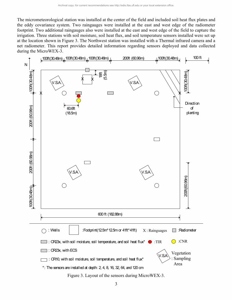
The majority of the gain in the system is provided by a gain and filtering block designed by the University of Michigan for the STAR-Light instrument (De Roo, 2003). The main advantage of this gain block is the close proximity of all the amplifiers, simplifying the task of thermal control. This gain block was designed for a radiometer working at the radio astronomy window of 1400 to 1427 MHz, and so the receiver is a heterodyne type with downconversion from the C-band RF to L-band. To minimize the receiver noise figure, a C-band low-noise amplifier (LNA) is used just prior to downconversion. To protect the amplifier from saturation due to out of band interference, a relatively wide bandwidth, but low insertion loss, bandpass filter is used just prior to the amplifier. Between the filter and the antenna are three components: a switch for choosing polarization, a switch for monitoring a reference load, and an isolator to minimize changes in the apparent system gain due to differences in the reflections looking upstream from the LNA. The electrical penetrations use commercially available weatherproof bulkhead connections (Deutsch connectors or equivalent). The heat sinks have been carefully located employing RTV (silicone sealant) to seal the bolt holes. The radome uses 15mil polycarbonate for radiometric signal penetration. It is sealed to the case using a rubber gasket held down to the case by a square retainer. The first SMA connection electomechanical latching, which is driven by the Z-World control board switches between V- and H-polarization sequentially. The SMA second latching which switches between the analog signal from the first switch and the reference load signal from a reference load resistor sends the analog signal to a isolator, where the signals within 6.4 to 7.2 GHz in radiofrequency are isolated. Then the central frequency is picked up by a 6.7 GHz bandpass filter, which also protects the amplifier to saturation. A Low Noise Amplifier (LNA) is used to eliminate the noise figure and adjust gain. A mixer takes the input from the LNA and a local oscillator to output a 1.4 GHz signal to STAR-Lite. After the Power Amplifier and Filtering Block (Star-Lite back-end), the signal is passed through a Square Law Detector and a Post-Detection Amplifier. UFCMR is equipped with a microcontroller that has responsibility for taking measurements, monitoring the thermal environment, and storing data until a download is requested. A labtop computer is used for running the user interface named FluxMon to communicate with the radiometer through Radiometer Control Language (RadiCL). The radiometer is configured to maintain a particular thermal set point, and make periodic measurements of the brightness at both polarizations sequentially and the reference load. The data collected by the radiometer is not calibrated within the instrument, since calibration errors could corrupt an otherwise useful dataset. Figure 5 shows the block diagram of UFCMR.
Archival copy: for current recommendations see http://edis.ifas.ufl.edu or your local extension office.
7
Figure 5. Block diagram of the University of Florida C-band Radiometer (De Roo, 2002).
4.2 Eddy Covariance System A Campbell Scientific eddy covariance system was located at the center of the field toward the north edge as shown in Figure 3. The system included a CSAT3 anemometer and KH20 hygrometer. Figure 6 shows a close up of the sensor. CSAT3 is a three dimensional sonic anemometer, which measures wind speed and the speed of sound on three non-orthogonal axes. Orthogonal wind speed and sonic temperature are computed from these measurements. KH20 measures the water vapor in the atmosphere. Its output voltage is proportional to the water vapor density flux. Latent and sensible heat fluxes were measured every 30 minutes. The height of the eddy covariance system was set to 2.1m in the beginning of experiment and was changed to 1.2 m on DoY 202, and the orientation of the system was 220° toward southwest. The height of the eddy covariance system was moved to 2.25 m from the ground on DoY 246. Table 2 shows the list of specifications of the CSAT3. Data collected by the eddy covariance system have been processed for coordinate rotation (Kaimal and Finnigan, 1994; Wilczak et al., 2001), WPL (Web et al., 1980), oxygen (van Dijk et al., 2003, 2004), and sonic temperature corrections (Schotanus et al., 1983). Figure A-2 shows the processed latent and sensible heat fluxes observed during MicroWEX-3.
Archival copy: for current recommendations see http://edis.ifas.ufl.edu or your local extension office.

8
Figure 6. Eddy covariance system
Table 2. Specifications of the CSAT3 (Campbell Scientific, 1998)
Description Value Measurement rate 1 to 60 Hz Noise equivalent wind 1 mm/sec in horizontal wind speed and 0.5 mm/sec in vertical wind speed Wind measurement offset < ±4 cm/sec over –30 to 50ºC Output signals Digital SDM or RS-232 and Analog Digital output signal range ±65.535 m/sec in wind speed and 300 to 366 m/sec in speed of sound Digital output signal resolution 0.25 to 2 mm/sec in vertical wind speed and 1 mm/s in speed of sound Analog output signal range ±32.768 to ±65.536 m/sec in wind speed and 300 to 366 m/sec in speed of sound Analog output signal resolution ±8.192 mm/sec in vertical wind speed and 16 mm/sec in speed of sound Measurement path length 10.0 cm vertical and 5.8 cm horizontal Transducer path angle from horizontal 60 degrees Transducer 0.64 cm in diameter Transducer mounting arms 0.84 cm in diameter Support arms 1.59 cm in diameter Dimensions: anemometer head 47.3 cm x 42.4 cm Dimensions: electronics box 26 cm x 16 cm x 9 cm Dimensions: carry case 71.1 cm x 58.4 cm x 33 cm Weight: anemometer head 1.7 kg Weight: electronics box 2.8 kg Weight: shipping 16.8 kg Operating temperature range -30ºC to 50ºC Power requirement: voltage supply 10 to 16 VDC Power requirement: current 200 mA at 60 Hz measurement rate and 100 mA at 20 Hz measurement rate
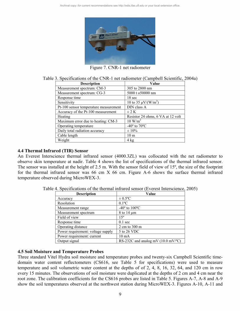
4.3 Net Radiometer A Kipp and Zonen CNR-1 four-component net radiometer (Figure 7) was located at the center of the field to measure up- and down-welling short- and long-wave infrared radiation. The sensor consists of two pyranometers (CM-3) and two pyrgeometers (CG-3). The sensor was installed at the height of 2.5 m above ground and facing south. Table 3 shows s the list of specifications of the CNR-1 net radiometer. Figure A-3 shows the up- and down-welling solar (shortwave) wave radiation observed during MicroWEX-3. Figure A-4 shows the up- and down-welling far infrared (longwave) radiation observedduringMicroWEX-3. Figure A-5 shows the net total radiation observed during MicrWEX-3.
Archival copy: for current recommendations see http://edis.ifas.ufl.edu or your local extension office.
9
Figure 7. CNR-1 net radiometer
Table 3. Specifications of the CNR-1 net radiometer (Campbell Scientific, 2004a)
Description Value Measurement spectrum: CM-3 305 to 2800 nm Measurement spectrum: CG-3 5000 t o50000 nm Response time 18 sec Sensitivity 10 to 35 μV/(W/m2) Pt-100 sensor temperature measurement DIN class A Accuracy of the Pt-100 measurement ± 2 K Heating Resistor 24 ohms, 6 VA at 12 volt Maximum error due to heating: CM-3 10 W/m2 Operating temperature -40º to 70ºC Daily total radiation accuracy ± 10% Cable length 10 m Weight 4 kg
4.4 Thermal Infrared (TIR) Sensor An Everest Interscience thermal infrared sensor (4000.3ZL) was collocated with the net radiometer to observe skin temperature at nadir. Table 4 shows the list of specifications of the thermal infrared sensor. The sensor was installed at the height of 2.5 m. With the sensor field of view of 15º, the size of the footprint for the thermal infrared sensor was 66 cm X 66 cm. Figure A-6 shows the surface thermal infrared temperature observed during MicroWEX-3.
Table 4. Specifications of the thermal infrared sensor (Everest Interscience, 2005) Description Value
Accuracy ± 0.5ºC Resolution 0.1ºC Measurement range -40º to 100ºC Measurement spectrum 8 to 14 µm Field of view 15º Response time 0.1 sec Operating distance 2 cm to 300 m Power requirement: voltage supply 5 to 26 VDC Power requirement: current 10 mA Output signal RS-232C and analog mV (10.0 mV/ºC)
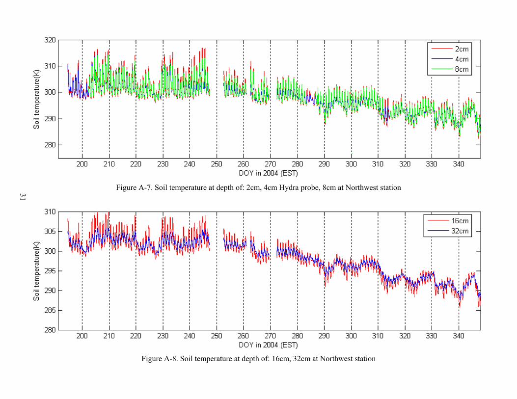
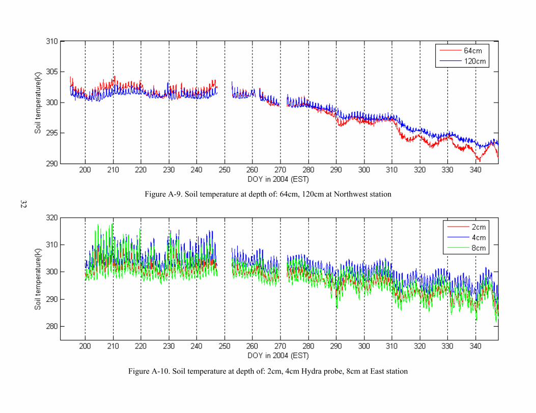
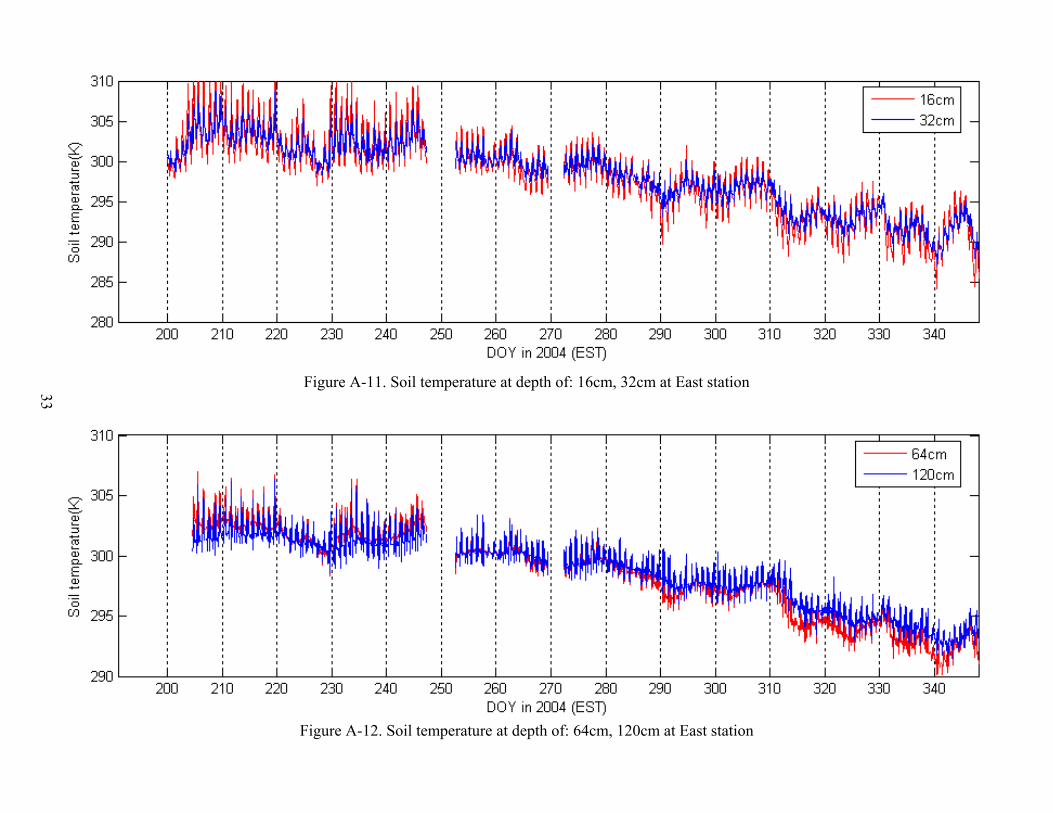
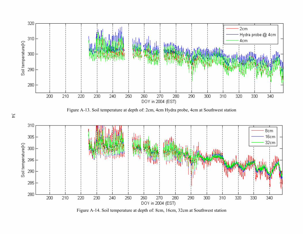
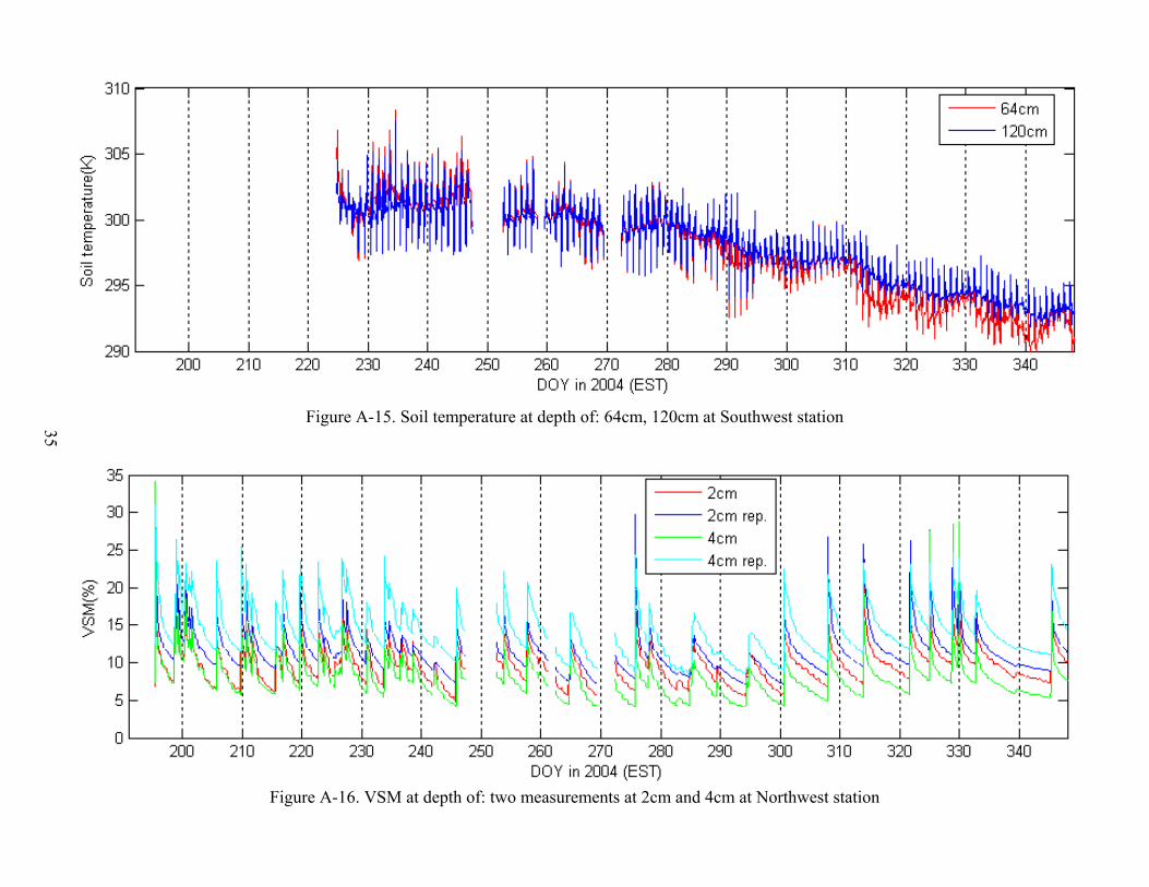
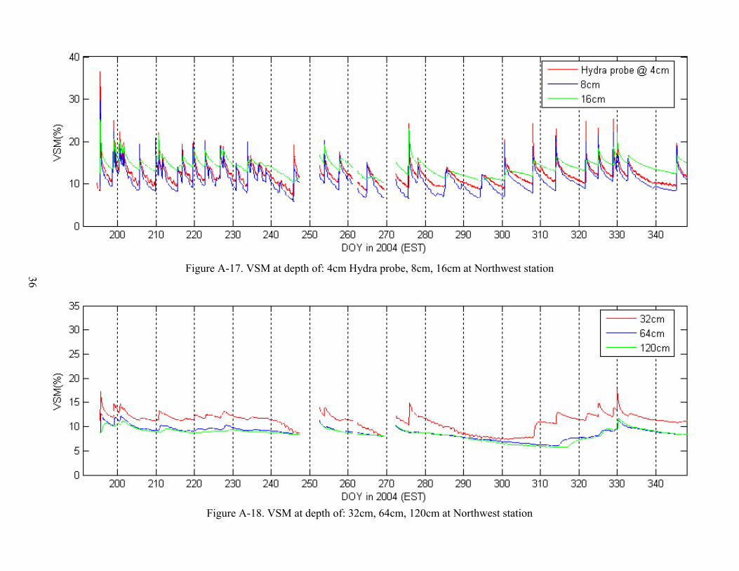
4.5 Soil Moisture and Temperature Probes Three standard Vitel Hydra soil moisture and temperature probes and twenty-six Campbell Scientific time-domain water content reflectometers (CS616, see Table 5 for specifications) were used to measure temperature and soil volumetric water content at the depths of of 2, 4, 8, 16, 32, 64, and 120 cm in row every 15 minutes. The observations of soil moisture were duplicated at the depths of 2 cm and 4 cm near the root zone. The calibration coefficients for the CS616 probes are listed in Table 5. Figures A-7, A-8 and A-9 show the soil temperatures observed at the northwest station during MicroWEX-3. Figures A-10, A-11 and
Archival copy: for current recommendations see http://edis.ifas.ufl.edu or your local extension office.
10
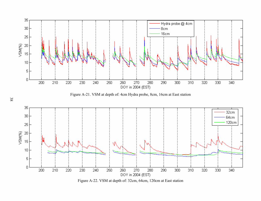
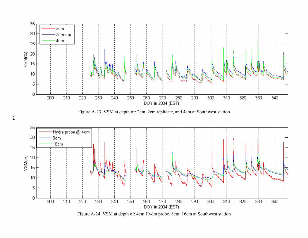
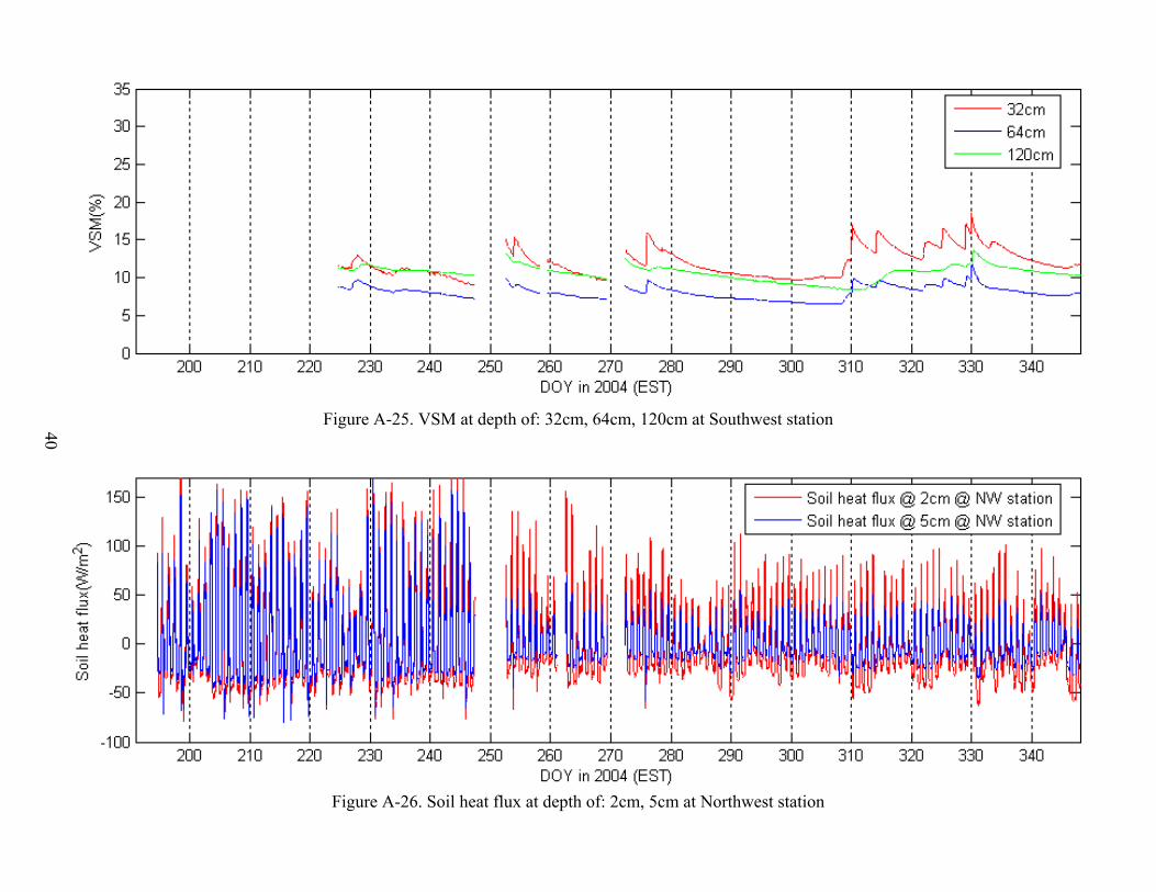
A-12 show the soil temperatures observed at the east station. Figures A-13, A-14 and A-15 show the soil temperatures observed at the southwest station. Figures A-16, A-17 and A-18 show the volumetric soil moisture content observed at the northwest station and Figure A-19 shows the volumetric soil moisture content observed at the depth of 1.7m located near the northwest monitoring well. Figures A-20, A-21 and A-22 show the volumetric soil moisture content observed at the east station. Figures A-23, A-24 and A-25 show the volumetric soil moisture content observed at the southwest station.
Table 5. The calibration coefficients for the CS616 probes (Campbell Scientific, 2004b) Coefficient Value
C0 -0.187 C1 0.037 C2 0.335
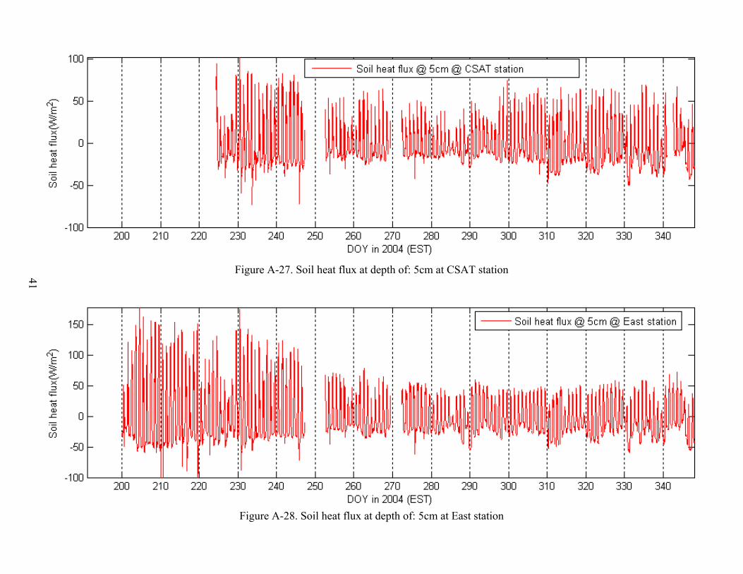
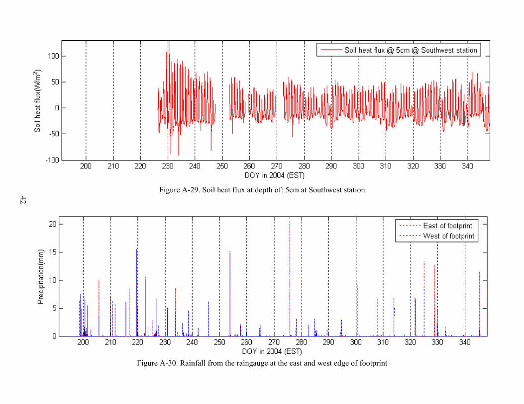
4.6 Soil Heat Flux Plates Two Campbell Scientific (2003) soil heat flux plates (HFT-3) were used to measure soil heat flux at the depths of 2 and 5 cm, in row and near the root area, respectively. Table 6 shows the list of specifications of the soil heat flux plate. Figure A-26 shows the soil heat fluxes observed at 2cm and 5cm at northwest station during MicroWEX-3. Figure A-27 shows the soil heat fluxes observed at 5cm at CSAT station. Figure A-28 shows the soil heat fluxes observed at 5cm at the east station. Figure A-29 shows the soil heat fluxes observed at 5cm at southwest station.
Table 6. Specifications of the soil heat flux plate (Campbell Scientific, 2003) Description Value
Operating temperature -40º to 55ºC Plate thickness 3.91 mm Plate diameter 38.2 mm Sensor Thermopile Measurement range ± 100 W/m2 Signal range ± 2.4 mV Accuracy ± 5% Thermal conductivity 1.22 W/m/K
4.7 Rain gauges Four rain gauges were installed in the field to measure the precipitation/irrigation. There were two rain gauges individually installed on the east and west edge of the footprint of the radiometer and were connected to the Northwest station. The amounts of precipitation/irrigation were recorded every 15 minutes. Figure A-30 shows the rainfall recorded by these two rain gauges. The other two rain gauges were set up on the east and west edge of the field and connected with Onset Hobo rainfall event datalogger to record the rainfall/irrigation. The time of every rainfall/irrigation event, which represents 0.2 mm of rainfall/irrigation, was recorded. Figure A-31 shows rainfall recorded by these rain gauges. 4.8 Canopy temperatures Six thermistors were installed in the canopy to measure the temperatures of canopy at 4 cm, 10 cm, 20 cm, 50 cm, 75 cm, and 90 cm. Perforated metal cans (painted white) were used as radiation shield to protect the sensor from direct sun and rain. Figure A-32 and A-33 show the canopy temperature at different heights.
5. SOIL SAMPLING
Extensive soil sampling was conducted to provide additional information of the spatial distribution of the surface soil moisture, temperature, and surface roughness. 5.1 Surface Roughness
Archival copy: for current recommendations see http://edis.ifas.ufl.edu or your local extension office.
11
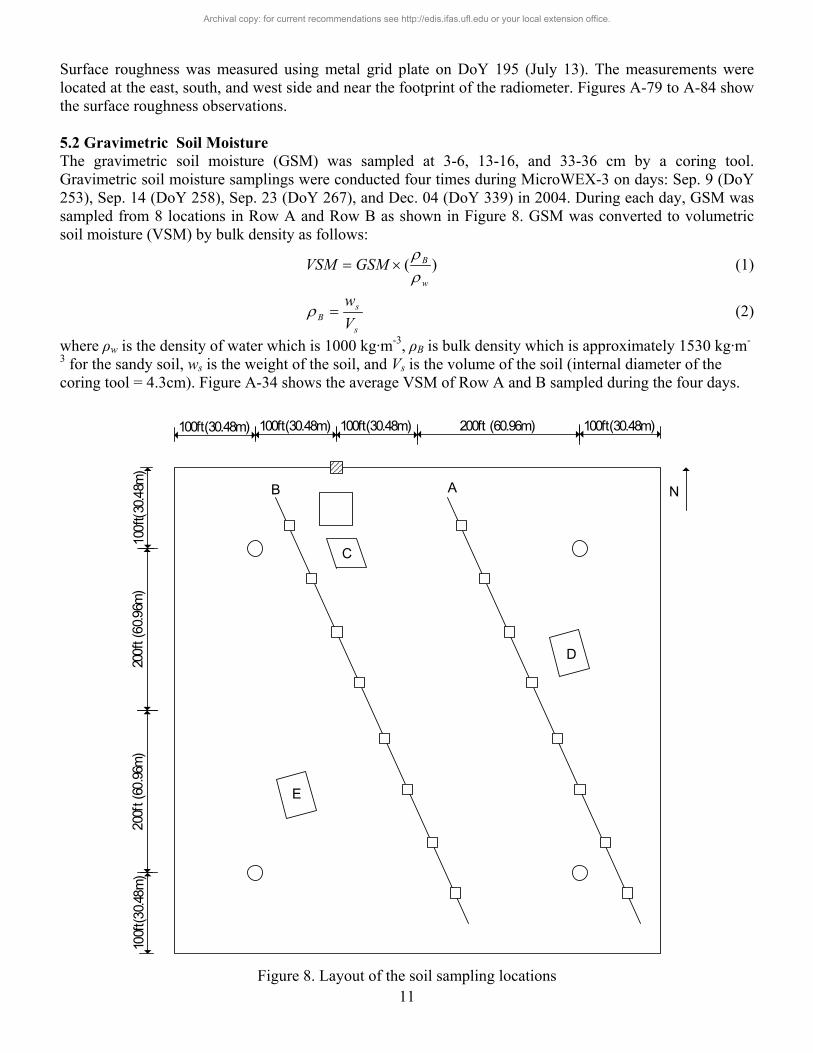
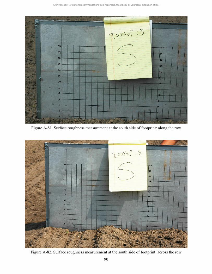
Surface roughness was measured using metal grid plate on DoY 195 (July 13). The measurements were located at the east, south, and west side and near the footprint of the radiometer. Figures A-79 to A-84 show the surface roughness observations. 5.2 Gravimetric Soil Moisture The gravimetric soil moisture (GSM) was sampled at 3-6, 13-16, and 33-36 cm by a coring tool. Gravimetric soil moisture samplings were conducted four times during MicroWEX-3 on days: Sep. 9 (DoY 253), Sep. 14 (DoY 258), Sep. 23 (DoY 267), and Dec. 04 (DoY 339) in 2004. During each day, GSM was sampled from 8 locations in Row A and Row B as shown in Figure 8. GSM was converted to volumetric soil moisture (VSM) by bulk density as follows:
)(w
BGSMVSMρρ
×= (1)
s
sB V
w=ρ (2)
where ρw is the density of water which is 1000 kg·m-3, ρB is bulk density which is approximately 1530 kg·m-
3 for the sandy soil, ws is the weight of the soil, and Vs is the volume of the soil (internal diameter of the coring tool = 4.3cm). Figure A-34 shows the average VSM of Row A and B sampled during the four days.
N
100ft(30.48m) 100ft(30.48m)100ft(30.48m)
100f
t(30.4
8m)
100f
t(30.4
8m)
200f
t (60
.96m
)20
0ft (
60.96
m)
200ft (60.96m)100ft(30.48m)
AB
D
C
E
Figure 8. Layout of the soil sampling locations
Archival copy: for current recommendations see http://edis.ifas.ufl.edu or your local extension office.
12
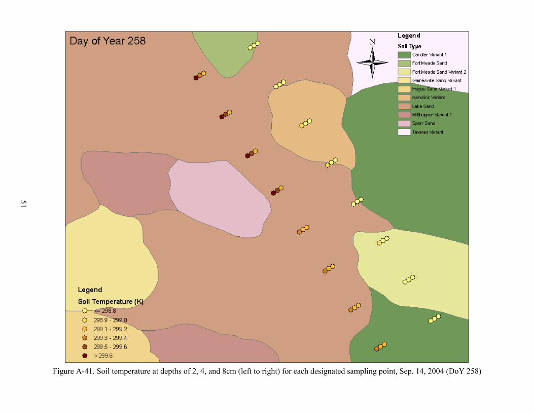
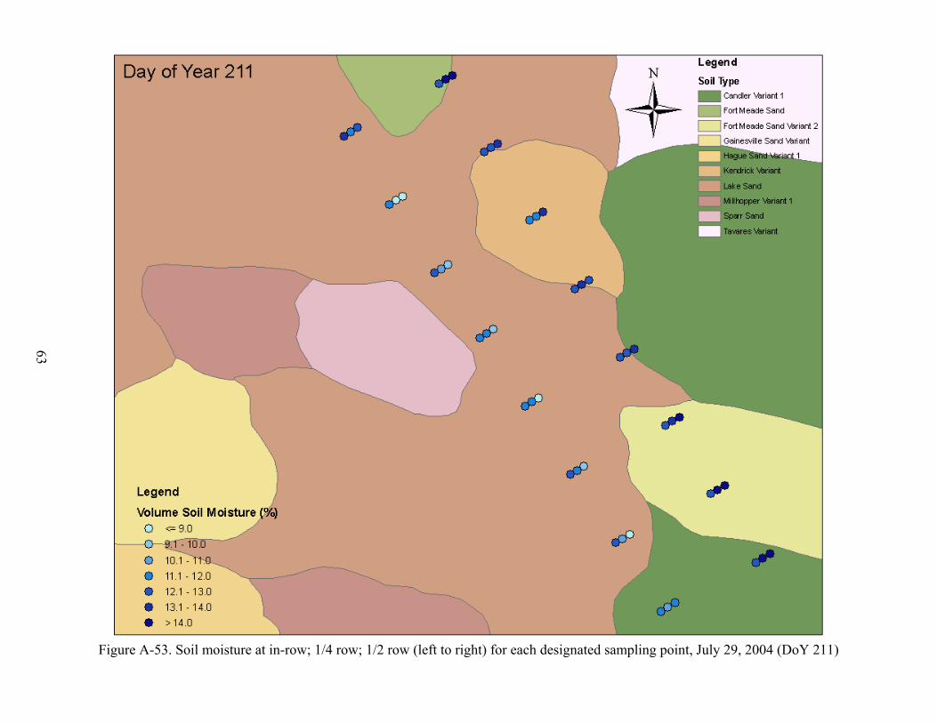
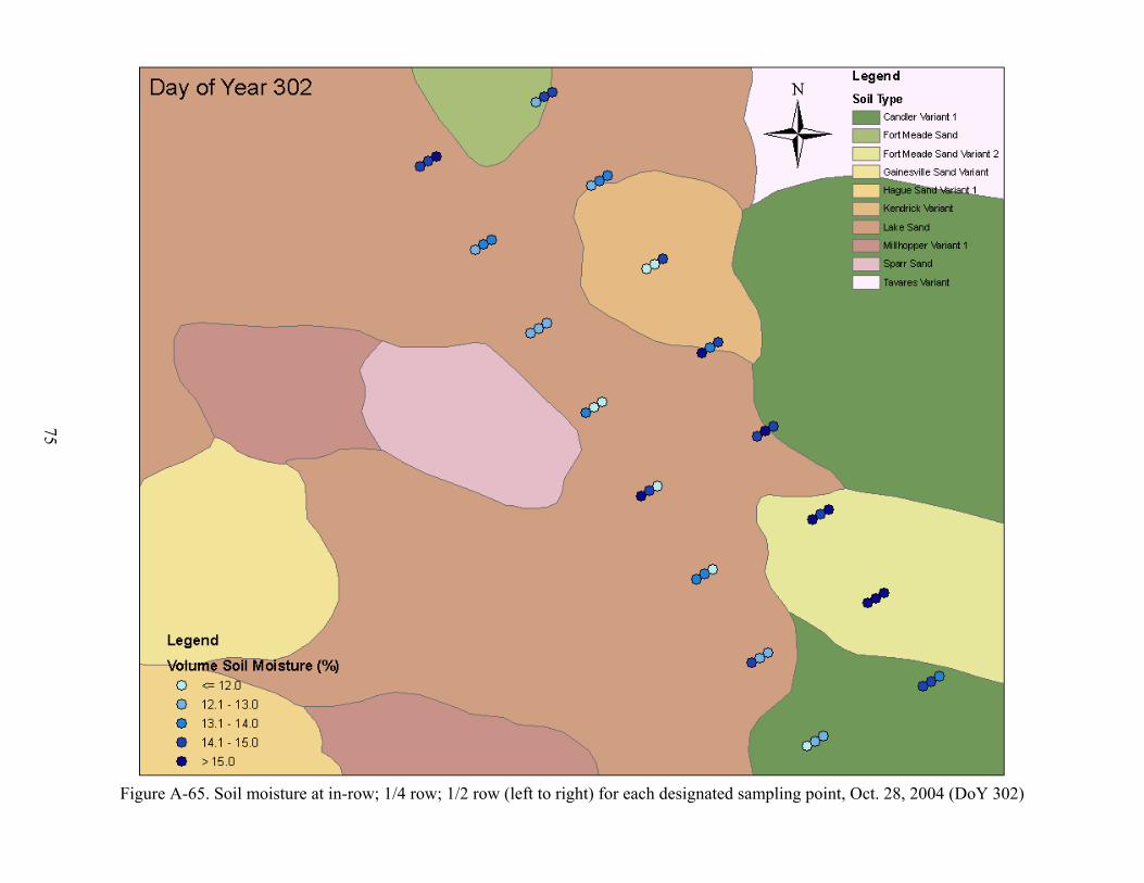
5.3 Soil Temperature A Max/Min waterproof digital thermometer from Forestry Supplier was used to measure the soil temperature at the depths of 2, 4, and 8 cm at locations A to E shown in Figure 8. An ML2 theta probe volumetric soil moisture sensor from Delta-T Devices was used to measure the soil moisture at the locations of in-row; 1/4 row; 1/2 row at the locations A to B shown in Figure 8. Figure A-35 to A-52 show soil temperature and figure A-53 to A-70 show soil moisture observed during the soil sampling.
6. VEGETATION SAMPLING
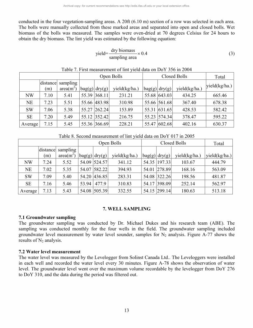
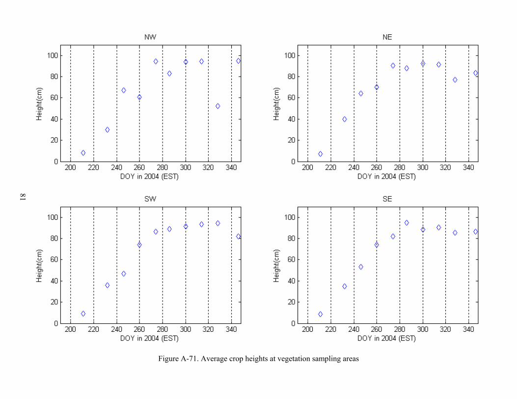
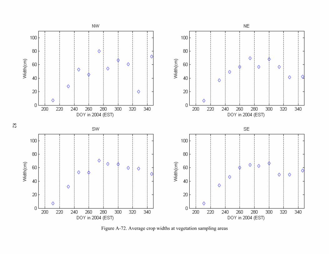
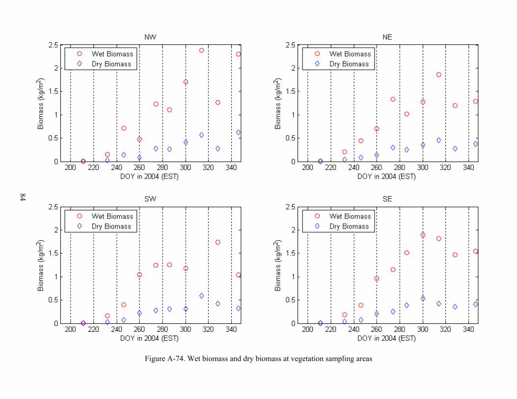
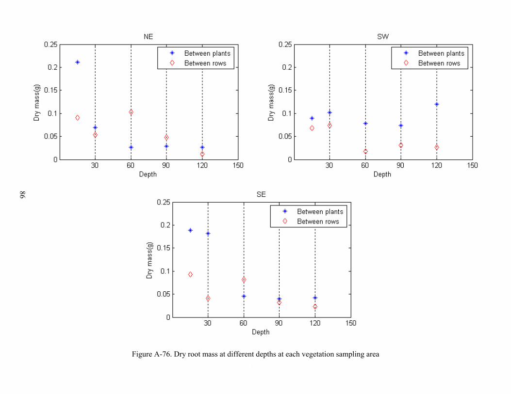
Vegetation properties such as stand density, row spacing, height, biomass, and LAI were measured bi-weekly during the field experiment. The crop density derived from the stand density and row spacing was measured during the first two sampling. The cotton seeds were planted in the fixed spacing and the germination rate is over 90% throughout the field. The bi-weekly measurements included height, width, biomass, LAI, and crop development. In the whole season, the vegetation samplings were conducted on four spatially distributed sampling locations (Figure 3) to characterize the spatial variability of vegetation properties in the study site. 6.1 Height and width Crop height was measured by placing a measuring tape at the soil surface to average height of the crop. The width was measured in the direction of maximum width. The heights inside the vegetation sampling areas were taken for each vegetation sampling. Figure A-71 to A-72 show the crop heights and widths during MicroWEX-3. 6.2 LAI LAI of the footprint was approximated by measuring 4 locations around the footprint bi-weekly. LAI was measured with a Li-Cor LAI-2000 in the inter-row region with 4 cross-row measurements. The LAI-2000 was set to average 4 locations into a single value so one observation was taken above the canopy and 4 beneath the canopy; in the row, ¼ of the way across the row, ½ of the way across the row, and ¾ of the way across the row. This gave a spatial average for row crops of partial cover. Figure A-73 shows the LAI observed during MicroWEX-3. 6.3 Green and Dry Biomass Each vegetation sampling was conducted along one row. The sampling length was measured the same as during stand density measurement. The plants within this length were cut at the base and put in plastic bags to prevent losing moisture. In the laboratory, the canopy samples were separated into leaves, stems, and bolls to measure their wet weights. The vegetation samples were put into paper bags and dried in the oven at 75ºC for 48 hours. Then the vegetation samples were removed from the oven and the dry weights were measured. At the time of harvest, lint yield was measured in certain area to estimate the yield of the whole field. Figure A-74 shows the wet biomass and dry biomass of different plant components observed during MicroWEX-3. 6.4 Root Sampling Root sampling was conducted in three of the four vegetation sampling areas (Northeast, Southeast, and Southwest). The root samples were taken at five depths: 0-15 cm, 15-30 cm, 30-60 cm, 60-90 cm, and 90-120 cm. The samples were then washed and scanned to obtain the structure of the roots. Figure A-75 shows the total root lengths at different depths. Figure A-76 shows the dry root mass at different depths. 6.5 Lint Yield The lint yield of cotton was estimated twice during MicroWEX-3. The first measurement was on DoY 356 (see Table 7) immediately after removal of sensors. The second time was on DoY 17 (see Table 8) in 2005, when harvest would have typically taken place based upon the numbers of open bolls. Harvest was
Archival copy: for current recommendations see http://edis.ifas.ufl.edu or your local extension office.
13
conducted in the four vegetation-sampling areas. A 20ft (6.10 m) section of a row was selected in each area. The bolls were manually collected from these marked areas and separated into open and closed bolls. Wet biomass of the bolls was measured. The samples were oven-dried at 70 degrees Celsius for 24 hours to obtain the dry biomass. The lint yield was estimated by the following equation:
dry biomassyield= 0.4sampling area
× (3)
Table 7. First measurement of lint yield data on DoY 356 in 2004
Open Bolls Closed Bolls Total
distance(m)
sampling area(m2) bag(g) dry(g) yield(kg/ha.) bag(g) dry(g) yield(kg/ha.) yield(kg/ha.)
NW 7.10 5.41 55.39 368.11 231.21 55.68 643.03 434.25 665.46 NE 7.23 5.51 55.66 483.98 310.98 55.66 561.68 367.40 678.38 SW 7.06 5.38 55.27 262.24 153.89 55.31 631.65 428.53 582.42 SE 7.20 5.49 55.12 352.42 216.75 55.23 574.34 378.47 595.22
Average 7.15 5.45 55.36 366.69 228.21 55.47 602.68 402.16 630.37
Table 8. Second measurement of lint yield data on DoY 017 in 2005 Open Bolls Closed Bolls Total
distance(m)
sampling area(m2) bag(g) dry(g) yield(kg/ha.) bag(g) dry(g) yield(kg/ha.) yield(kg/ha.)
NW 7.24 5.52 54.09 524.57 341.12 54.35 197.33 103.67 444.79 NE 7.02 5.35 54.07 582.22 394.93 54.01 278.89 168.16 563.09 SW 7.09 5.40 54.20 436.85 283.31 54.08 322.26 198.56 481.87 SE 7.16 5.46 53.94 477.9 310.83 54.17 398.09 252.14 562.97
Average 7.13 5.43 54.08 505.39 332.55 54.15 299.14 180.63 513.18
7. WELL SAMPLING
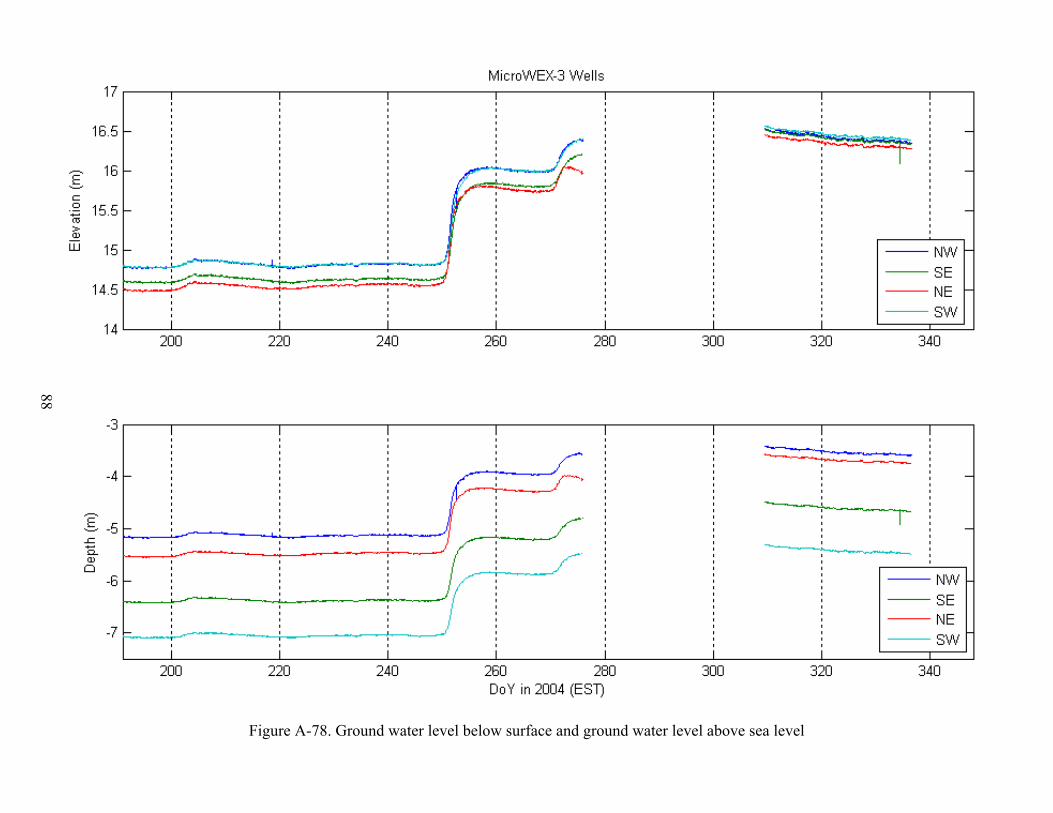
7.1 Groundwater sampling The groundwater sampling was conducted by Dr. Michael Dukes and his research team (ABE). The sampling was conducted monthly for the four wells in the field. The groundwater sampling included groundwater level measurement by water level sounder, samples for N2 analysis. Figure A-77 shows the results of N2 analysis. 7.2 Water level measurement The water level was measured by the Levelogger from Solinst Canada Ltd.. The Leveloggers were installed in each well and recorded the water level every 30 minutes. Figure A-78 shows the observation of water level. The groundwater level went over the maximum volume recordable by the levelogger from DoY 276 to DoY 310, and the data during the period was filtered out.
Archival copy: for current recommendations see http://edis.ifas.ufl.edu or your local extension office.

14
8. FIELD LOG
Note: Time is in Eastern Standard Time.
The cotton was planted on June 21 (DoY173). Root fungus destroyed the seedlings. Cotton was re-planted on July 09 (DoY 191). The field log below was generated from July 09 (DoY191). There were three hurricanes during MicroWEX-3. The UFCMR was disconnected in order to prevent possible damages. UFCMR was overheated once during MicroWEX-3. The events and data gaps for UFCMR are listed in Table 9:
Table 9. The events and dates of data gaps for UFCMR during MicroWEX-3 Event Hurricane Charley Hurricane Frances Hurricane Jeanne Overheating Dates Aug. 14, DoY 227 Sep. 06, DoY 250 Sep. 26, DoY 270 Nov. 02, DoY 307
Dates of data gap DoY 225-229 DoY 247-253 DoY 269-273 DoY 307-309 The stations of dataloggers were also disconnected to power supply during the hurricanes. The data gaps of stations of dataloggers are listed in Table 10 below:
Table 10. The events and dates of data gaps of dataloggers at Northwest, East, and Southwest stations during MicroWEX-3
Event Hurricane Frances Hurricane Jeanne Dates Sep. 06, DoY 250 Sep. 26, DoY 270
Dates of data gap DoY 247-253 DoY 269-273 July 09 (DoY 191)
07:10 Land preparation, finished at 11:30 08:30 Planting, 09:30 to 11:50, 12:40 to 15:00
July 12 (DoY 194)
07:30 Marked the footprint of radiometer 08:00 Set up tripods for all dataloggers 09:30 Connected sensors to Northwest station ( by Miller) 10:30 Connected sensors to East station ( by Miller)
July 13 (DoY 195)
09:30 Set up TIR, CNR, and CSAT ( by Lanni and Miller), the cal.# of CSAT is -0.206, the height of CSAT was 2.1 m.
10:30 Surface roughness measurement near footprint Cotton germination observed
July 14 (DoY 196)
08:30 Buried the sensors at East station 10:30 Measurement of the height of CNR(2.66m), TIR(2.5m)
July 19 (DoY 201)
07:30 Set up raingauges at the east and west edge of field 10:30 The #2 thermistor (at 8cm) at Northwest station was not
working due to broken cable, fixed on DoY 202
Archival copy: for current recommendations see http://edis.ifas.ufl.edu or your local extension office.
15
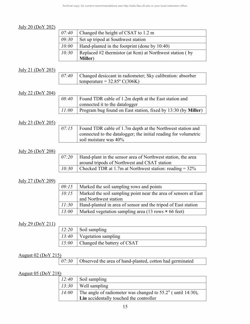
July 20 (DoY 202)
07:40 Changed the height of CSAT to 1.2 m 09:30 Set up tripod at Southwest station 10:00 Hand-planted in the footprint (done by 10:40) 10:30 Replaced #2 thermistor (at 8cm) at Northwest station ( by
Miller) July 21 (DoY 203)
07:40 Changed desiccant in radiometer; Sky calibration: absorber temperature = 32.85º C(306K)
July 22 (DoY 204)
08:40 Found TDR cable of 1.2m depth at the East station and connected it to the datalogger
11:00 Program bug found on East station, fixed by 13:30 (by Miller) July 23 (DoY 205)
07:15 Found TDR cable of 1.7m depth at the Northwest station and connected to the datalogger; the initial reading for volumetric soil moisture was 40%
July 26 (DoY 208)
07:20 Hand-plant in the sensor area of Northwest station, the area around tripods of Northwest and CSAT station
10:30 Checked TDR at 1.7m at Northwest station: reading = 32% July 27 (DoY 209)
09:15 Marked the soil sampling rows and points 10:15 Marked the soil sampling point near the area of sensors at East
and Northwest station 11:30 Hand-planted in area of sensor and the tripod of East station 13:00 Marked vegetation sampling area (13 rows × 66 feet)
July 29 (DoY 211)
12:20 Soil sampling 13:40 Vegetation sampling 15:00 Changed the battery of CSAT
August 02 (DoY 215)
07:30 Observed the area of hand-planted, cotton had germinated August 05 (DoY 218)
12:40 Soil sampling 13:30 Well sampling 14:00 The angle of radiometer was changed to 55.2° ( until 14:30),
Lin accidentally touched the controller
Archival copy: for current recommendations see http://edis.ifas.ufl.edu or your local extension office.

16
August 09 (DoY 222)
08:05 Changed desiccant in radiometer; Sky calibration: absorber temperature = 30.30º (303.45K)
August 11 (DoY 224)
07:30 Connected sensors to Southwest station, done by 14:45 ( by Miller)
07:30 Buried sensors at Southwest station (by Lin) 15:00 Connected soil heat flux sensor to CSAT station ( by Miller)
August 12 (DoY 225)
08:00 Soil sampling 11:30 Shut down radiometer (preparation of Hurricane Charley)
August 13 (DoY 226)
07:30 Connected soil heat flux sensor to Southwest station, done by 7:50
08:00 Uploaded new program to Southwest station August 16 (DoY 229)
08:00 Turned on the radiometer power on 08:30 Replaced battery of CSAT 09:00 Modified the program of Southwest station; find #1 thermistor
(at 2cm) not working, fixed on DoY 232 09:30 Started the radiometer to take reading
August 19 (DoY 232)
13:00 Replaced KH2O with the one from Dr. Jacobs ( by Miller), the cal.# is -0.185
13:30 Soil sampling 14:30 Vegetation sampling 15:00 Modified the program at Northwest station (by Tien)
August 20 (DoY 233)
08:30 Connected thermistors #3~#8 (for canopy temperature, at 4cm, 10cm, 20cm, 50cm, 75cm, and 90cm) at Northwest station, done by 10:00
10:00 Found #4 thermo-couple (at 120 cm) at Northwest station not working, fixed at DoY 234
10:30 LAI measurement 12:00 Program bug found at Northwest station ( by Miller)
August 21 (DoY 234)
06:20 Uploaded the new program at Northwest station to fix the problem of #4 thermo-couple
Cotton square observed
Archival copy: for current recommendations see http://edis.ifas.ufl.edu or your local extension office.
17
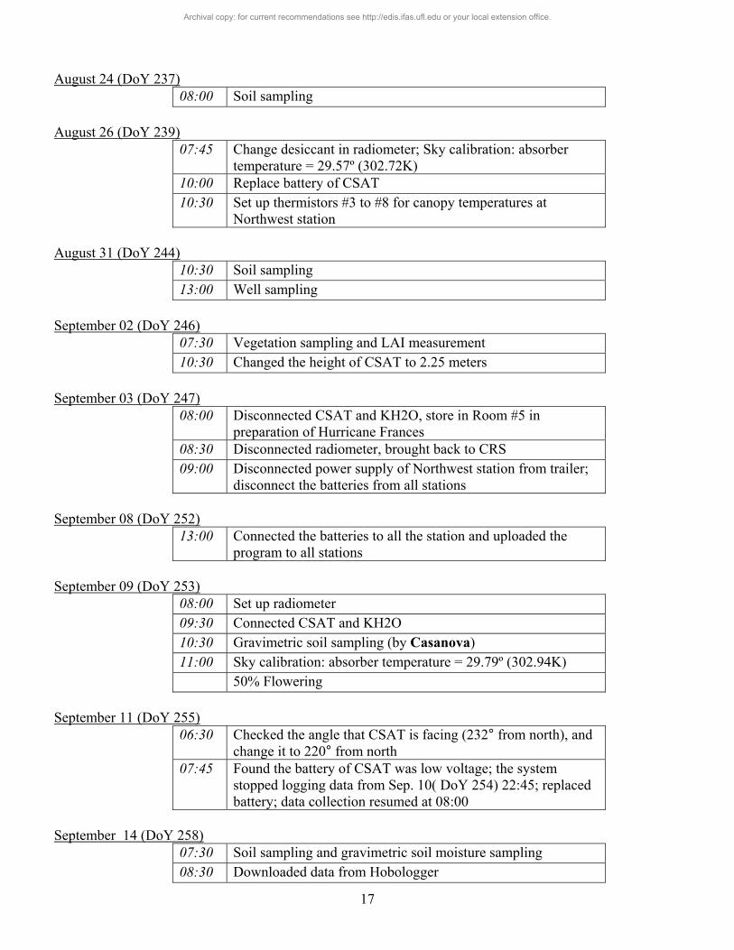
August 24 (DoY 237)
08:00 Soil sampling August 26 (DoY 239)
07:45 Change desiccant in radiometer; Sky calibration: absorber temperature = 29.57º (302.72K)
10:00 Replace battery of CSAT 10:30 Set up thermistors #3 to #8 for canopy temperatures at
Northwest station August 31 (DoY 244)
10:30 Soil sampling 13:00 Well sampling
September 02 (DoY 246)
07:30 Vegetation sampling and LAI measurement 10:30 Changed the height of CSAT to 2.25 meters
September 03 (DoY 247)
08:00 Disconnected CSAT and KH2O, store in Room #5 in preparation of Hurricane Frances
08:30 Disconnected radiometer, brought back to CRS 09:00 Disconnected power supply of Northwest station from trailer;
disconnect the batteries from all stations September 08 (DoY 252)
13:00 Connected the batteries to all the station and uploaded the program to all stations
September 09 (DoY 253)
08:00 Set up radiometer 09:30 Connected CSAT and KH2O 10:30 Gravimetric soil sampling (by Casanova) 11:00 Sky calibration: absorber temperature = 29.79º (302.94K) 50% Flowering
September 11 (DoY 255)
06:30 Checked the angle that CSAT is facing (232° from north), and change it to 220° from north
07:45 Found the battery of CSAT was low voltage; the system stopped logging data from Sep. 10( DoY 254) 22:45; replaced battery; data collection resumed at 08:00
September 14 (DoY 258)
07:30 Soil sampling and gravimetric soil moisture sampling 08:30 Downloaded data from Hobologger
Archival copy: for current recommendations see http://edis.ifas.ufl.edu or your local extension office.

18
Observed 70% to 80% of cotton with flower September 15 (DoY 259)
07:30 Replaced the KH2O with the one of CRS (disconnected the one from Dr. Jacobs and stored in Room#5), the cal.# is -0.206
September 16 (DoY 260)
07:30 Vegetation sampling and LAI measurement 09:00 Found the battery of CSAT was low voltage; the system
stopped logging data from Sep. 16( DoY 260) 06:00; replace battery, data collection resumed at 10:30
September 18 (DoY 262)
08:00 Found the battery of Northwest station was low voltage; the system stopped logging data from Sep. 17( DoY 261) 00:45; connected the power cable; data collection resumed at 09:00
September 20 (DoY 264)
13:30 Replaced battery of CSAT September 23 (DoY 267)
07:30 Soil sampling and gravimetric soil moisture sampling 09:00 Conducted Cropscan in northeast vegetation sampling area 10:00 Checked the battery of CSAT (12.8 volt)
September 25 (DoY 269)
06:30 Found the battery of CSAT was low voltage; the system stopped logging data from Sep. 24 ( DoY 268) 16:30; replace battery
08:00 Shut down radiometer in preparation of Hurricane Jeanne 10:30 Disconnected all batteries from all stations; disconnect all
power supply cable 12:00 Disconnected radiometer and brought back to CRS 12:30 Disconnected KH2O and CSAT and stored in Room #5 at Pine
Acres September 28 (DoY 272)
07:00 Connected all batteries to the stations and reload the programs 08:00 Soil sampling 09:00 Connected CSAT and KH2O Observed 10% to 15% of cotton with bolls The radiometer could not be started because the booting
sequence of radiometer and laptop was mistaken September 29 (DoY 273)
13:00 Changed desiccant in radiometer and reboot radiometer 13:30 Sky calibration: absorber temperature = 33.4° (306.55K)
Archival copy: for current recommendations see http://edis.ifas.ufl.edu or your local extension office.

19
14:15 Staredt the radiometer to log data 15:00 Replace dbattery of CSAT
September 30 (DoY 274)
07:30 Vegetation sampling and LAI measurement October 01 (DoY 275)
14:50 Well sampling October 02 (DoY 276)
08:30 Replaced battery of CSAT The groundwater level went over the range of the levelogger.
Data filtered October 07 (DoY 281)
08:00 Soil sampling Observed 35% to 45% of cotton with bolls
October 09 (DoY 283)
08:30 Found the power supply pole broken due to vehicle operation; took pictures; verified the power supply is working
October 12 (DoY 286)
09:30 Vegetation sampling and LAI measurement October 14 (DoY 288)
07:15 Soil sampling 08:30 Conducted Cropscan in northeast and northwest vegetation
sampling area Observed 50% of cotton with bolls
October 19 (DoY 293)
09:30 Sky calibration: absorber temperature = 30.66° (303.81K) October 21 (DoY 295)
07:30 Soil sampling 08:00 Modifyied the program of Southwest station and added a
reference temperature sensor ( by Miller) October 23 (DoY 297)
06:30 Replaced battery of CSAT 08:00 Downloaded data from Hobologger
October 26 (DoY 300)
09:30 Vegetation sampling and LAI measurement Observed open bolls from the cotton that first planted on June
21 (DoY 173)
Archival copy: for current recommendations see http://edis.ifas.ufl.edu or your local extension office.
20
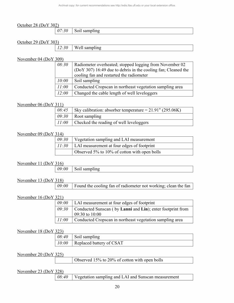
October 28 (DoY 302)
07:30 Soil sampling October 29 (DoY 303)
12:30 Well sampling November 04 (DoY 309)
08:30 Radiometer overheated; stopped logging from November 02 (DoY 307) 16:49 due to debris in the cooling fan; Cleaned the cooling fan and restarted the radiometer
10:00 Soil sampling 11:00 Conducted Cropscan in northeast vegetation sampling area 12:00 Changed the cable length of well leveloggers
November 06 (DoY 311)
08:45 Sky calibration: absorber temperature = 21.91° (295.06K) 09:30 Root sampling 11:00 Checked the reading of well leveloggers
November 09 (DoY 314)
09:30 Vegetation sampling and LAI measurement 11:30 LAI measurement at four edges of footprint Observed 5% to 10% of cotton with open bolls
November 11 (DoY 316)
09:00 Soil sampling November 13 (DoY 318)
09:00 Found the cooling fan of radiometer not working; clean the fan November 16 (DoY 321)
09:00 LAI measurement at four edges of footprint 09:30 Conducted Sunscan ( by Lanni and Lin); enter footprint from
09:30 to 10:00 11:00 Conducted Cropscan in northeast vegetation sampling area
November 18 (DoY 323)
08:40 Soil sampling 10:00 Replaced battery of CSAT
November 20 (DoY 325)
Observed 15% to 20% of cotton with open bolls November 23 (DoY 328)
08:40 Vegetation sampling and LAI and Sunscan measurement
Archival copy: for current recommendations see http://edis.ifas.ufl.edu or your local extension office.
21
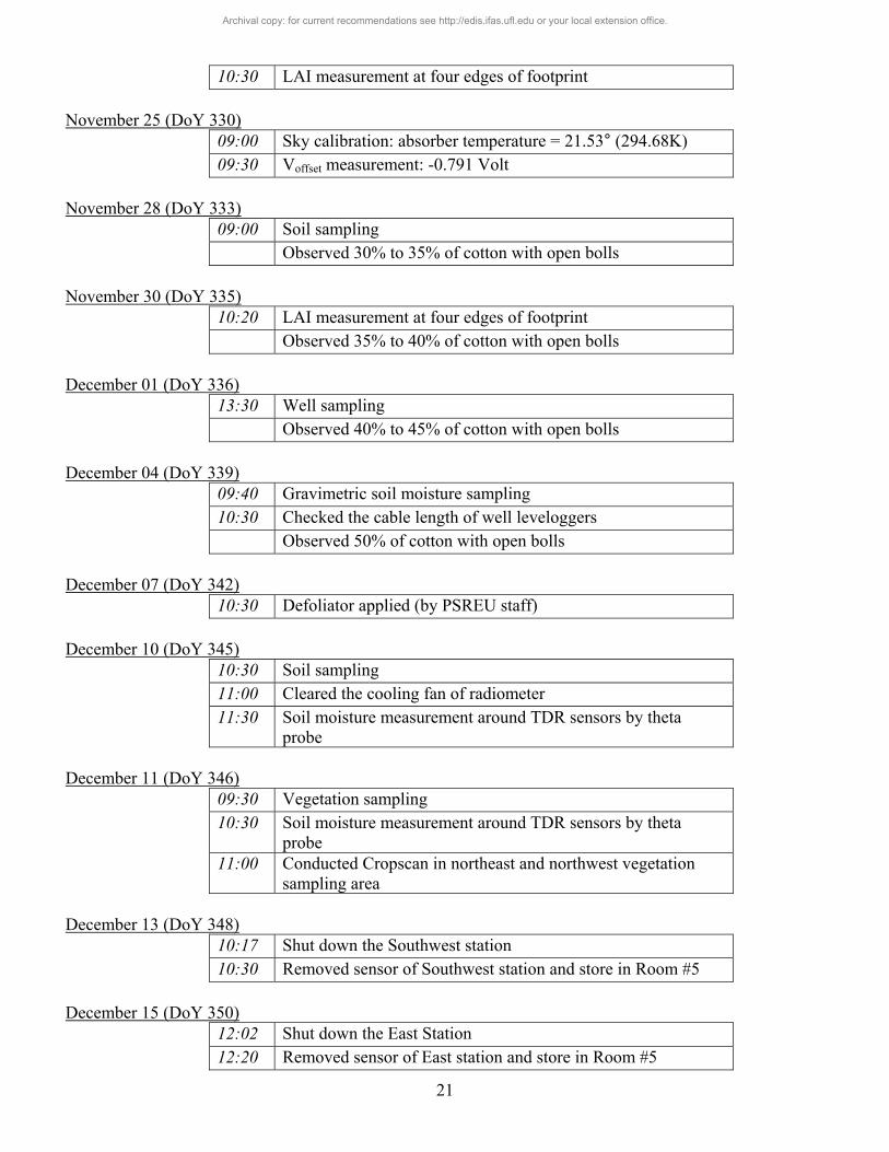
10:30 LAI measurement at four edges of footprint November 25 (DoY 330)
09:00 Sky calibration: absorber temperature = 21.53° (294.68K) 09:30 Voffset measurement: -0.791 Volt
November 28 (DoY 333)
09:00 Soil sampling Observed 30% to 35% of cotton with open bolls
November 30 (DoY 335)
10:20 LAI measurement at four edges of footprint Observed 35% to 40% of cotton with open bolls
December 01 (DoY 336)
13:30 Well sampling Observed 40% to 45% of cotton with open bolls
December 04 (DoY 339)
09:40 Gravimetric soil moisture sampling 10:30 Checked the cable length of well leveloggers Observed 50% of cotton with open bolls
December 07 (DoY 342)
10:30 Defoliator applied (by PSREU staff) December 10 (DoY 345)
10:30 Soil sampling 11:00 Cleared the cooling fan of radiometer 11:30 Soil moisture measurement around TDR sensors by theta
probe December 11 (DoY 346)
09:30 Vegetation sampling 10:30 Soil moisture measurement around TDR sensors by theta
probe 11:00 Conducted Cropscan in northeast and northwest vegetation
sampling area December 13 (DoY 348)
10:17 Shut down the Southwest station 10:30 Removed sensor of Southwest station and store in Room #5
December 15 (DoY 350)
12:02 Shut down the East Station 12:20 Removed sensor of East station and store in Room #5
Archival copy: for current recommendations see http://edis.ifas.ufl.edu or your local extension office.
22
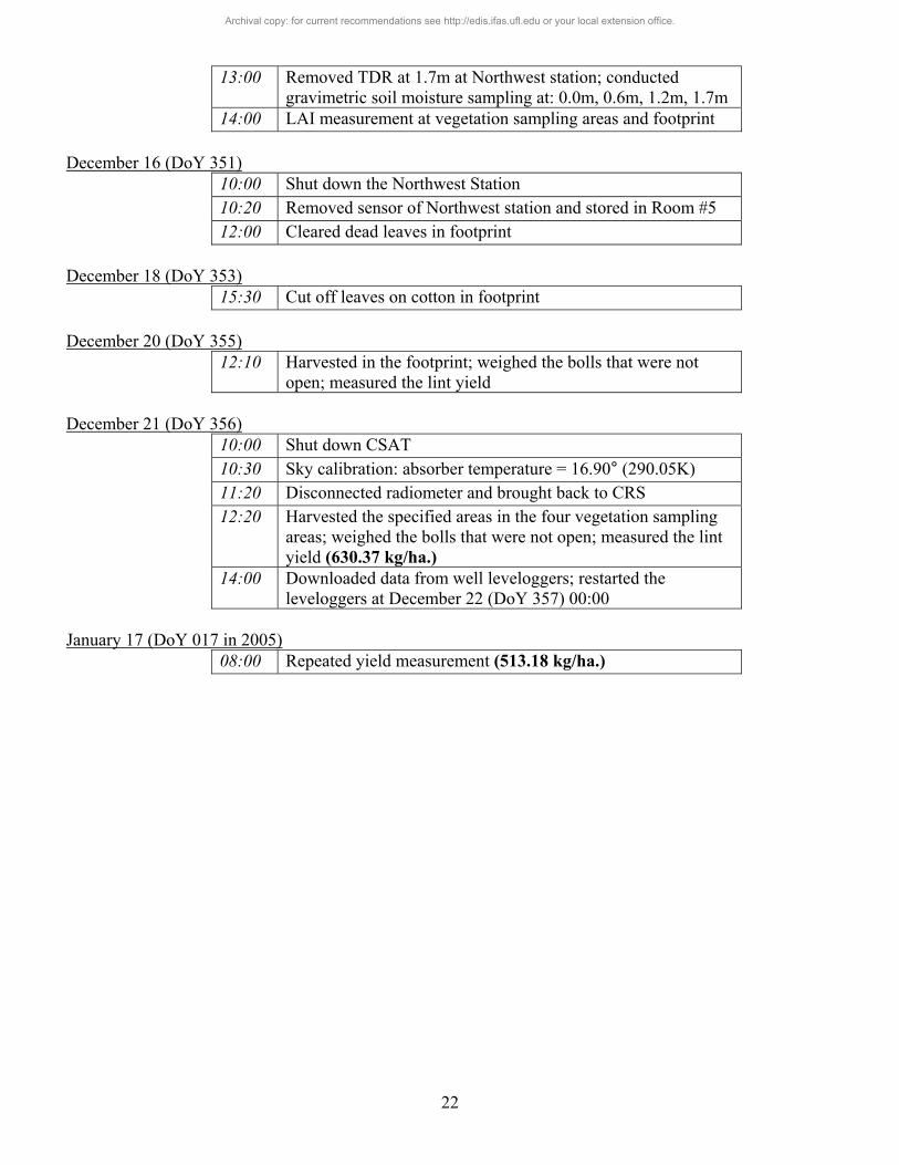
13:00 Removed TDR at 1.7m at Northwest station; conducted gravimetric soil moisture sampling at: 0.0m, 0.6m, 1.2m, 1.7m
14:00 LAI measurement at vegetation sampling areas and footprint December 16 (DoY 351)
10:00 Shut down the Northwest Station 10:20 Removed sensor of Northwest station and stored in Room #5 12:00 Cleared dead leaves in footprint
December 18 (DoY 353)
15:30 Cut off leaves on cotton in footprint December 20 (DoY 355)
12:10 Harvested in the footprint; weighed the bolls that were not open; measured the lint yield
December 21 (DoY 356)
10:00 Shut down CSAT 10:30 Sky calibration: absorber temperature = 16.90° (290.05K) 11:20 Disconnected radiometer and brought back to CRS 12:20 Harvested the specified areas in the four vegetation sampling
areas; weighed the bolls that were not open; measured the lint yield (630.37 kg/ha.)
14:00 Downloaded data from well leveloggers; restarted the leveloggers at December 22 (DoY 357) 00:00
January 17 (DoY 017 in 2005)
08:00 Repeated yield measurement (513.18 kg/ha.)
Archival copy: for current recommendations see http://edis.ifas.ufl.edu or your local extension office.
23
ACKNOWLEDGEMENT The authors would like to acknowledge Mr. James Boyer and his team at the PSREU, Citra, Florida for excellent field management. We also thank Dr. Wendy Graham, Dr. James Jones, and Dr. Jennifer Jacobs for their scientific advice in experimental design. MicroWEX-3 was supported by grant from the Earth Science Directorate of the NSF (Grant number: EAR-0337277).
REFERENCES
Campbell Scientific, CSAT3 Three Dimensional Sonic Anemometer Instruction Manual, Campbell Scientific Inc., Logan, UT, 1998.
Campbell Scientific, HFT3 soil heat flux plate instruction manual, Campbell Scientific Inc., Logan, UT,
2003. Campbell Scientific, CNR1 Net Radiometer Instruction Manual, Campbell Scientific Inc., Logan, UT,
2004a. Campbell Scientific, CS615 andCS625 water content reflectometers instruction manual, Campbell
Scientific Inc., Logan, UT, 2004b. Everest Interscience, Model 4000.3ZL Infrared Temperature Sensor, Everest Interscience Inc., Tuson, AZ,
2005. J. C. Kaimal and J. J. Finnigan, Atmospheric Boundary Layer Flows, Oxford University Press, New York,
NY, 1994. R. D. De Roo, University of Florida C-band Radiometer Summary, Space Physics Research Laboratory,
University of Michigan, Ann Arbor, MI, March, 2002. R. D. D Roo, TMR-3 Radiometer Tuning Procedures, Space Physics Research Laboratory, University of
Michigan, Ann Arbor, MI, March, 2003. P. Schotanus, F. T. M. Nieuwstadt, and H. A. R. DeBruin, “Temperature measurement with a sonic
anemometer and its application to heat and moisture fluctuations,” Bound.-Layer Meteorol., vol. 26, pp. 81-93, 1983.
A. van Dijk, W. Kohsiek, and H. A. R. DeBruin, “Oxygen sensitivity of krypton and Lyman-alpha
hygrometer,” J. Atmos. Ocean. Tech., vol. 20, pp. 143-151., 2003. A. van Dijk, A. F. Moene, and H. A. R. DeBurin, The Principles of Surface Flux Physics: Theory, Practice,
and Description of the ECPACK Library, http://www.met.wau.nl/projects/jep/, 2004. E. K. Webb, G. I. Pearman, and R. Leuning, “ Correction of flux measurements for density effects due to
heat and water vapor transfer,” Quart. J. Roy. Meteorol., Soc., vol. 106, pp. 85-100, 1980. J. M. Wilczak, S. P. Oncley, and S. A. Stage, “Sonic anemometer tilt correction algorithms,” Bound.-Layer
Meteorol., vol. 99, pp. 127-150, 2001.
Archival copy: for current recommendations see http://edis.ifas.ufl.edu or your local extension office.
24
A. FIELD OBSERVATIONS
Figure Captions Figure A-1. Brightness temperatures at vertical and horizontal polarizations ……………………… 28 Figure A-2. Latent (LE) and sensible (H) heat fluxes ……………………………………………… 28 Figure A-3. Down- and up-welling solar radiation ………………………………………………… 29 Figure A-4. Down- and up-welling far infrared radiation ………………………………………… 29 Figure A-5. Total net radiation …………………………………………………………………… 30 Figure A-6. Surface temperature …………………………………………………………………… 30 Figure A-7. Soil temperature at depth of: 2cm, 4cm Hydra probe, 8cm at Northwest station ……… 31 Figure A-8. Soil temperature at depth of: 16cm, 32cm at Northwest station ……………………… 31 Figure A-9. Soil temperature at depth of: 64cm, 120cm at Northwest station ……………………… 32 Figure A-10. Soil temperature at depth of: 2cm, 4cm Hydra probe, 8cm at East station ………… 32 Figure A-11. Soil temperature at depth of: 16cm, 32cm at East station …………………………… 33 Figure A-12. Soil temperature at depth of: 64cm, 120cm at East station ………………………… 33 Figure A-13. Soil temperature at depth of: 2cm, 4cm Hydra probe, 4cm at Southwest station……… 34 Figure A-14. Soil temperature at depth of: 8cm, 16cm, 32cm at Southwest station ……………… 34 Figure A-15. Soil temperature at depth of: 64cm, 120cm at Southwest station …………………… 35 Figure A-16. VSM at depth of: two measurements at 2cm and 4cm at Northwest station ………… 35 Figure A-17. VSM at depth of: 4cm Hydra probe, 8cm, 16cm at Northwest station ……………… 36 Figure A-18. VSM at depth of: 32cm, 64cm, 120cm at Northwest station ………………………… 36 Figure A-19. VSM at depth of: 1.7m near Northwest monitoring well at Northwest station ……… 37 Figure A-20. VSM at depth of: 2cm, 2cm replicate, and 4cm at East station ……………………… 37 Figure A-21. VSM at depth of: 4cm Hydra probe, 8cm, 16cm at East station ……………………… 38 Figure A-22. VSM at depth of: 32cm, 64cm, 120cm at East station ……………………………… 38 Figure A-23. VSM at depth of: 2cm, 2cm replicate, and 4cm at Southwest station ……………… 39 Figure A-24. VSM at depth of: 4cm Hydra probe, 8cm, 16cm at Southwest station ……………… 39 Figure A-25. VSM at depth of: 32cm, 64cm, 120cm at Southwest station ………………………… 40 Figure A-26. Soil heat flux at depth of: 2cm, 5cm at Northwest station …………………………… 40 Figure A-27. Soil heat flux at depth of: 5cm at CSAT station ……………………………………… 41 Figure A-28. Soil heat flux at depth of: 5cm at East station ………………………………………… 41 Figure A-29. Soil heat flux at depth of: 5cm at Southwest station ………………………………… 42 Figure A-30. Rainfall from the raingauge at the east and west edge of footprint ………………… 42 Figure A-31. Rainfall from the raingauge at the east and west edge of the field …………………… 43 Figure A-32. Canopy temperature at 4 cm, 10 cm, 20 cm ………………………………………… 43 Figure A-33. Canopy temperature at 50 cm, 75 cm, and 90 cm …………………………………… 44 Figure A-34. VSM at specific sampling points …………………………………………………… 44
Archival copy: for current recommendations see http://edis.ifas.ufl.edu or your local extension office.
25
Figure A-35. Soil temperature at depths of 2, 4, and 8cm (left to right) for each designated sampling point, July 29, 2004 (DoY 211) ………… 45
Figure A-36. Soil temperature at depths of 2, 4, and 8cm (left to right) for each designated sampling point, Aug. 05, 2004 (DoY 218) ………… 46
Figure A-37. Soil temperature at depths of 2, 4, and 8cm (left to right) for each designated sampling point, Aug. 12, 2004 (DoY 225) ………… 47
Figure A-38. Soil temperature at depths of 2, 4, and 8cm (left to right) for each designated sampling point, Aug. 19, 2004 (DoY 232) ………… 48
Figure A-39. Soil temperature at depths of 2, 4, and 8cm (left to right) for each designated sampling point, Aug. 24, 2004 (DoY 237) ………… 49
Figure A-40. Soil temperature at depths of 2, 4, and 8cm (left to right) for each designated sampling point, Aug. 31, 2004 (DoY 244) ………… 50
Figure A-41. Soil temperature at depths of 2, 4, and 8cm (left to right) for each designated sampling point, Sep. 14, 2004 (DoY 258) ………… 51
Figure A-42. Soil temperature at depths of 2, 4, and 8cm (left to right) for each designated sampling point, Sep. 23, 2004 (DoY 267) ………… 52
Figure A-43. Soil temperature at depths of 2, 4, and 8cm (left to right) for each designated sampling point, Sep. 28, 2004 (DoY 272) ………… 53
Figure A-44. Soil temperature at depths of 2, 4, and 8cm (left to right) for each designated sampling point, Oct. 07, 2004 (DoY 281) ………… 54
Figure A-45. Soil temperature at depths of 2, 4, and 8cm (left to right) for each designated sampling point, Oct. 14, 2004 (DoY 288) ………… 55
Figure A-46. Soil temperature at depths of 2, 4, and 8cm (left to right) for each designated sampling point, Oct. 21, 2004 (DoY 295) ………… 56
Figure A-47. Soil temperature at depths of 2, 4, and 8cm (left to right) for each designated sampling point, Oct. 28, 2004 (DoY 302) ………… 57
Figure A-48. Soil temperature at depths of 2, 4, and 8cm (left to right) for each designated sampling point, Nov. 04, 2004 (DoY 309) ………… 58
Figure A-49. Soil temperature at depths of 2, 4, and 8cm (left to right) for each designated sampling point, Nov. 11, 2004 (DoY 316) ………… 59
Figure A-50. Soil temperature at depths of 2, 4, and 8cm (left to right) for each designated sampling point, Nov. 18, 2004 (DoY 323) ………… 60
Figure A-51. Soil temperature at depths of 2, 4, and 8cm (left to right) for each designated sampling point, Nov. 28, 2004 (DoY 333) ………… 61
Figure A-52. Soil temperature at depths of 2, 4, and 8cm (left to right) for each designated sampling point, Dec. 10, 2004 (DoY 345) ………… 62
Archival copy: for current recommendations see http://edis.ifas.ufl.edu or your local extension office.
26
Figure A-53. Soil moisture at in-row; 1/4 row; 1/2 row (left to right) for each designated sampling point, July 29, 2004 (DoY 211) …………… 63
Figure A-54. Soil moisture at in-row; 1/4 row; 1/2 row (left to right) for each designated sampling point, Aug. 05, 2004 (DoY 218) …………… 64
Figure A-55. Soil moisture at in-row; 1/4 row; 1/2 row (left to right) for each designated sampling point, Aug. 12, 2004 (DoY 225) …………… 65
Figure A-56. Soil moisture at in-row; 1/4 row; 1/2 row (left to right) for each designated sampling point, Aug. 19, 2004 (DoY 232) …………… 66
Figure A-57. Soil moisture at in-row; 1/4 row; 1/2 row (left to right) for each designated sampling point, Aug. 24, 2004 (DoY 237) …………… 67
Figure A-58. Soil moisture at in-row; 1/4 row; 1/2 row (left to right) for each designated sampling point, Aug. 31, 2004 (DoY 244) …………… 68
Figure A-59. Soil moisture at in-row; 1/4 row; 1/2 row (left to right) for each designated sampling point, Sep. 14, 2004 (DoY 258) …………… 69
Figure A-60. Soil moisture at in-row; 1/4 row; 1/2 row (left to right) for each designated sampling point, Sep. 23, 2004 (DoY 267) …………… 70
Figure A-61. Soil moisture at in-row; 1/4 row; 1/2 row (left to right) for each designated sampling point, Sep. 28, 2004 (DoY 272) …………… 71
Figure A-62. Soil moisture at in-row; 1/4 row; 1/2 row (left to right) for each designated sampling point, Oct. 07, 2004 (DoY 281) …………… 72
Figure A-63. Soil moisture at in-row; 1/4 row; 1/2 row (left to right) for each designated sampling point, Oct. 14, 2004 (DoY 288) …………… 73
Figure A-64. Soil moisture at in-row; 1/4 row; 1/2 row (left to right) for each designated sampling point, Oct. 21, 2004 (DoY 295) …………… 74
Figure A-65. Soil moisture at in-row; 1/4 row; 1/2 row (left to right) for each designated sampling point, Oct. 28, 2004 (DoY 302) …………… 75
Figure A-66. Soil moisture at in-row; 1/4 row; 1/2 row (left to right) for each designated sampling point, Nov. 04, 2004 (DoY 309) …………… 76
Figure A-67. Soil moisture at in-row; 1/4 row; 1/2 row (left to right) for each designated sampling point, Nov. 11, 2004 (DoY 316) …………… 77
Figure A-68. Soil moisture at in-row; 1/4 row; 1/2 row (left to right) for each designated sampling point, Nov. 18, 2004 (DoY 323) …………… 78
Figure A-69. Soil moisture at in-row; 1/4 row; 1/2 row (left to right) for each designated sampling point, Nov. 28, 2004 (DoY 333) …………… 79
Figure A-70. Soil moisture at in-row; 1/4 row; 1/2 row (left to right) for each designated sampling point, Dec. 10, 2004 (DoY 345) …………… 80
Archival copy: for current recommendations see http://edis.ifas.ufl.edu or your local extension office.

27
Figure A-71. Average crop heights at vegetation sampling areas ………………………………… 81 Figure A-72. Average crop widths at vegetation sampling areas …………………………………… 82 Figure A-73. LAI at vegetation sampling areas …………………………………………………… 83 Figure A-74. Wet biomass and dry biomass at vegetation sampling areas ………………………… 84 Figure A-75. Total root length at different depths at each vegetation sampling area ……………… 85 Figure A-76. Dry root mass at different depths at each vegetation sampling area ………………… 86 Figure A-77. NO4 concentration at the monitoring wells …………………………………………… 87 Figure A-78. Ground water level below surface and ground water level above sea level ………… 88 Figure A-79. Surface roughness at the east side of the footprint: along the row …………………… 89 Figure A-80. Surface roughness at the east side of the footprint: across the row …………………… 89 Figure A-81. Surface roughness at the south side of the footprint: along the row ………………… 90 Figure A-82. Surface roughness at the south side of the footprint: across the row ………………… 90 Figure A-83. Surface roughness at the west side of the footprint: along the row ………………… 91 Figure A-84. Surface roughness at the west side of the footprint: across the row ………………… 91
Archival copy: for current recommendations see http://edis.ifas.ufl.edu or your local extension office.

Figure A-1. Brightness temperatures at vertically and horizontally polarizations
Figure A-2 Latent (LE) and sensible (H) heat fluxes
28
Archival copy: for current recommendations see http://edis.ifas.ufl.edu or your local extension office.

29
Figure A-3. Down- and up-welling solar radiation
Figure A-4. Down- and up-welling far infrared radiation
29
Archival copy: for current recommendations see http://edis.ifas.ufl.edu or your local extension office.

30
Figure A-5. Total net radiation
Figure A-6. Surface temperature
30
Archival copy: for current recommendations see http://edis.ifas.ufl.edu or your local extension office.
31
Figure A-7. Soil temperature at depth of: 2cm, 4cm Hydra probe, 8cm at Northwest station
Figure A-8. Soil temperature at depth of: 16cm, 32cm at Northwest station
31
Archival copy: for current recommendations see http://edis.ifas.ufl.edu or your local extension office.
32
Figure A-9. Soil temperature at depth of: 64cm, 120cm at Northwest station
Figure A-10. Soil temperature at depth of: 2cm, 4cm Hydra probe, 8cm at East station
32
Archival copy: for current recommendations see http://edis.ifas.ufl.edu or your local extension office.
33
Figure A-11. Soil temperature at depth of: 16cm, 32cm at East station
Figure A-12. Soil temperature at depth of: 64cm, 120cm at East station
33
Archival copy: for current recommendations see http://edis.ifas.ufl.edu or your local extension office.
34
Figure A-13. Soil temperature at depth of: 2cm, 4cm Hydra probe, 4cm at Southwest station
Figure A-14. Soil temperature at depth of: 8cm, 16cm, 32cm at Southwest station
34
Archival copy: for current recommendations see http://edis.ifas.ufl.edu or your local extension office.
35
Figure A-15. Soil temperature at depth of: 64cm, 120cm at Southwest station
Figure A-16. VSM at depth of: two measurements at 2cm and 4cm at Northwest station
35
Archival copy: for current recommendations see http://edis.ifas.ufl.edu or your local extension office.
36
Figure A-17. VSM at depth of: 4cm Hydra probe, 8cm, 16cm at Northwest station
Figure A-18. VSM at depth of: 32cm, 64cm, 120cm at Northwest station
36
Archival copy: for current recommendations see http://edis.ifas.ufl.edu or your local extension office.

37
Figure A-19. VSM at depth of: 1.7m near Northwest monitoring well at Northwest station
Figure A-20. VSM at depth of: 2cm, 2cm replicate, and 4cm at East station
37
Archival copy: for current recommendations see http://edis.ifas.ufl.edu or your local extension office.
38
Figure A-21. VSM at depth of: 4cm Hydra probe, 8cm, 16cm at East station
Figure A-22. VSM at depth of: 32cm, 64cm, 120cm at East station
38
Archival copy: for current recommendations see http://edis.ifas.ufl.edu or your local extension office.
39
Figure A-23. VSM at depth of: 2cm, 2cm replicate, and 4cm at Southwest station
Figure A-24. VSM at depth of: 4cm Hydra probe, 8cm, 16cm at Southwest station
39
Archival copy: for current recommendations see http://edis.ifas.ufl.edu or your local extension office.
40
Figure A-25. VSM at depth of: 32cm, 64cm, 120cm at Southwest station
Figure A-26. Soil heat flux at depth of: 2cm, 5cm at Northwest station
40
Archival copy: for current recommendations see http://edis.ifas.ufl.edu or your local extension office.
41
Figure A-27. Soil heat flux at depth of: 5cm at CSAT station
Figure A-28. Soil heat flux at depth of: 5cm at East station
41
Archival copy: for current recommendations see http://edis.ifas.ufl.edu or your local extension office.
42
Figure A-29. Soil heat flux at depth of: 5cm at Southwest station
Figure A-30. Rainfall from the raingauge at the east and west edge of footprint
42
Archival copy: for current recommendations see http://edis.ifas.ufl.edu or your local extension office.

43
Figure A-31. Rainfall from the raingauge at the east and west edge of the field
Figure A-32. Canopy temperature at 4 cm, 10 cm, 20 cm
43
Archival copy: for current recommendations see http://edis.ifas.ufl.edu or your local extension office.

44
Figure A-33. Canopy temperature at 50 cm, 75 cm, and 90 cm
Figure A-34. VSM at specific sampling points in Row A and Row B
44
Archival copy: for current recommendations see http://edis.ifas.ufl.edu or your local extension office.

45
Figure A-35. Soil temperature at depths of 2, 4, and 8cm (left to right) for each designated sampling point, July 29, 2004 (DoY 211)
45
Archival copy: for current recommendations see http://edis.ifas.ufl.edu or your local extension office.

46
Figure A-36. Soil temperature at depths of 2, 4, and 8cm (left to right) for each designated sampling point, Aug. 05, 2004 (DoY 218)
46
Archival copy: for current recommendations see http://edis.ifas.ufl.edu or your local extension office.

47
Figure A-37. Soil temperature at depths of 2, 4, and 8cm (left to right) for each designated sampling point, Aug. 12, 2004 (DoY 225)
47
Archival copy: for current recommendations see http://edis.ifas.ufl.edu or your local extension office.

48
Figure A-38. Soil temperature at depths of 2, 4, and 8cm (left to right) for each designated sampling point, Aug. 19, 2004 (DoY 232)
48
Archival copy: for current recommendations see http://edis.ifas.ufl.edu or your local extension office.

49
Figure A-39. Soil temperature at depths of 2, 4, and 8cm (left to right) for each designated sampling point, Aug. 24, 2004 (DoY 237)
49
Archival copy: for current recommendations see http://edis.ifas.ufl.edu or your local extension office.

50
Figure A-40. Soil temperature at depths of 2, 4, and 8cm (left to right) for each designated sampling point, Aug. 31, 2004 (DoY 244)
50
Archival copy: for current recommendations see http://edis.ifas.ufl.edu or your local extension office.
51
Figure A-41. Soil temperature at depths of 2, 4, and 8cm (left to right) for each designated sampling point, Sep. 14, 2004 (DoY 258)
51
Archival copy: for current recommendations see http://edis.ifas.ufl.edu or your local extension office.

52
Figure A-42. Soil temperature at depths of 2, 4, and 8cm (left to right) for each designated sampling point, Sep. 23, 2004 (DoY 267)
52
Archival copy: for current recommendations see http://edis.ifas.ufl.edu or your local extension office.

53
Figure A-43. Soil temperature at depths of 2, 4, and 8cm (left to right) for each designated sampling point, Sep. 28, 2004 (DoY 272)
53
Archival copy: for current recommendations see http://edis.ifas.ufl.edu or your local extension office.

54
Figure A-44. Soil temperature at depths of 2, 4, and 8cm (left to right) for each designated sampling point, Oct. 07, 2004 (DoY 281)
54
Archival copy: for current recommendations see http://edis.ifas.ufl.edu or your local extension office.

55
Figure A-45. Soil temperature at depths of 2, 4, and 8cm (left to right) for each designated sampling point, Oct. 14, 2004 (DoY 288)
55
Archival copy: for current recommendations see http://edis.ifas.ufl.edu or your local extension office.

56
Figure A-46. Soil temperature at depths of 2, 4, and 8cm (left to right) for each designated sampling point, Oct. 21, 2004 (DoY 295)
56
Archival copy: for current recommendations see http://edis.ifas.ufl.edu or your local extension office.

57
Figure A-47. Soil temperature at depths of 2, 4, and 8cm (left to right) for each designated sampling point, Oct. 28, 2004 (DoY 302)
57
Archival copy: for current recommendations see http://edis.ifas.ufl.edu or your local extension office.

58
Figure A-48. Soil temperature at depths of 2, 4, and 8cm (left to right) for each designated sampling point, Nov. 04, 2004 (DoY 309)
58
Archival copy: for current recommendations see http://edis.ifas.ufl.edu or your local extension office.

59
Figure A-49. Soil temperature at depths of 2, 4, and 8cm (left to right) for each designated sampling point, Nov. 11, 2004 (DoY 316)
59
Archival copy: for current recommendations see http://edis.ifas.ufl.edu or your local extension office.

60
Figure A-50. Soil temperature at depths of 2, 4, and 8cm (left to right) for each designated sampling point, Nov. 18, 2004 (DoY 323)
60
Archival copy: for current recommendations see http://edis.ifas.ufl.edu or your local extension office.

61
Figure A-51. Soil temperature at depths of 2, 4, and 8cm (left to right) for each designated sampling point, Nov. 28, 2004 (DoY 333)
61
Archival copy: for current recommendations see http://edis.ifas.ufl.edu or your local extension office.

62
Figure A-52. Soil temperature at depths of 2, 4, and 8cm (left to right) for each designated sampling point, Dec. 10, 2004 (DoY 345)
62
Archival copy: for current recommendations see http://edis.ifas.ufl.edu or your local extension office.
63
Figure A-53. Soil moisture at in-row; 1/4 row; 1/2 row (left to right) for each designated sampling point, July 29, 2004 (DoY 211)
63
Archival copy: for current recommendations see http://edis.ifas.ufl.edu or your local extension office.

64
Figure A-54. Soil moisture at in-row; 1/4 row; 1/2 row (left to right) for each designated sampling point, Aug. 05, 2004 (DoY 218)
64
Archival copy: for current recommendations see http://edis.ifas.ufl.edu or your local extension office.

65
Figure A-55. Soil moisture at in-row; 1/4 row; 1/2 row (left to right) for each designated sampling point, Aug. 12, 2004 (DoY 225)
65
Archival copy: for current recommendations see http://edis.ifas.ufl.edu or your local extension office.

66
Figure A-56. Soil moisture at in-row; 1/4 row; 1/2 row (left to right) for each designated sampling point, Aug. 19, 2004 (DoY 232)
66
Archival copy: for current recommendations see http://edis.ifas.ufl.edu or your local extension office.

67
Figure A-57. Soil moisture at in-row; 1/4 row; 1/2 row (left to right) for each designated sampling point, Aug. 24, 2004 (DoY 237)
67
Archival copy: for current recommendations see http://edis.ifas.ufl.edu or your local extension office.

68
Figure A-58. Soil moisture at in-row; 1/4 row; 1/2 row (left to right) for each designated sampling point, Aug. 31, 2004 (DoY 244)
68
Archival copy: for current recommendations see http://edis.ifas.ufl.edu or your local extension office.

69
Figure A-59. Soil moisture at in-row; 1/4 row; 1/2 row (left to right) for each designated sampling point, Sep. 14, 2004 (DoY 258)
69
Archival copy: for current recommendations see http://edis.ifas.ufl.edu or your local extension office.

70
Figure A-60. Soil moisture at in-row; 1/4 row; 1/2 row (left to right) for each designated sampling point, Sep. 23, 2004 (DoY 267)
70
Archival copy: for current recommendations see http://edis.ifas.ufl.edu or your local extension office.

71
Figure A-61. Soil moisture at in-row; 1/4 row; 1/2 row (left to right) for each designated sampling point, Sep. 28, 2004 (DoY 272)
71
Archival copy: for current recommendations see http://edis.ifas.ufl.edu or your local extension office.

72
Figure A-62. Soil moisture at in-row; 1/4 row; 1/2 row (left to right) for each designated sampling point, Oct. 07, 2004 (DoY 281)
72
Archival copy: for current recommendations see http://edis.ifas.ufl.edu or your local extension office.

73
Figure A-63. Soil moisture at in-row; 1/4 row; 1/2 row (left to right) for each designated sampling point, Oct. 14, 2004 (DoY 288)
73
Archival copy: for current recommendations see http://edis.ifas.ufl.edu or your local extension office.

74
Figure A-64. Soil moisture at in-row; 1/4 row; 1/2 row (left to right) for each designated sampling point, Oct. 21, 2004 (DoY 295)
74
Archival copy: for current recommendations see http://edis.ifas.ufl.edu or your local extension office.
75
Figure A-65. Soil moisture at in-row; 1/4 row; 1/2 row (left to right) for each designated sampling point, Oct. 28, 2004 (DoY 302)
75
Archival copy: for current recommendations see http://edis.ifas.ufl.edu or your local extension office.

76
Figure A-66. Soil moisture at in-row; 1/4 row; 1/2 row (left to right) for each designated sampling point, Nov. 04, 2004 (DoY 309)
76
Archival copy: for current recommendations see http://edis.ifas.ufl.edu or your local extension office.

77
Figure A-67. Soil moisture at in-row; 1/4 row; 1/2 row (left to right) for each designated sampling point, Nov. 11, 2004 (DoY 316)
77
Archival copy: for current recommendations see http://edis.ifas.ufl.edu or your local extension office.

78
Figure A-68. Soil moisture at in-row; 1/4 row; 1/2 row (left to right) for each designated sampling point, Nov. 18, 2004 (DoY 323)
78
Archival copy: for current recommendations see http://edis.ifas.ufl.edu or your local extension office.

79
Figure A-69. Soil moisture at in-row; 1/4 row; 1/2 row (left to right) for each designated sampling point, Nov. 28, 2004 (DoY 333)
79
Archival copy: for current recommendations see http://edis.ifas.ufl.edu or your local extension office.

80
Figure A-70. Soil moisture at in-row; 1/4 row; 1/2 row (left to right) for each designated sampling point, Dec. 10, 2004 (DoY 345)
80
Archival copy: for current recommendations see http://edis.ifas.ufl.edu or your local extension office.
81
Figure A-71. Average crop heights at vegetation sampling areas
81
Archival copy: for current recommendations see http://edis.ifas.ufl.edu or your local extension office.
82
Figure A-72. Average crop widths at vegetation sampling areas
82
Archival copy: for current recommendations see http://edis.ifas.ufl.edu or your local extension office.

83
Figure A-73. LAI at vegetation sampling areas
83
Archival copy: for current recommendations see http://edis.ifas.ufl.edu or your local extension office.
84
Figure A-74. Wet biomass and dry biomass at vegetation sampling areas
84
Archival copy: for current recommendations see http://edis.ifas.ufl.edu or your local extension office.

85
Figure A-75. Total root length at different depths at each vegetation sampling area
85
Archival copy: for current recommendations see http://edis.ifas.ufl.edu or your local extension office.
86
Figure A-76. Dry root mass at different depths at each vegetation sampling area
86
Archival copy: for current recommendations see http://edis.ifas.ufl.edu or your local extension office.

87
Figure A-77. NO4 concentration at the monitoring wells
87
Archival copy: for current recommendations see http://edis.ifas.ufl.edu or your local extension office.
88
Figure A-78. Ground water level below surface and ground water level above sea level
88
Archival copy: for current recommendations see http://edis.ifas.ufl.edu or your local extension office.

89
Figure A-79. Surface roughness measurement at the east side of footprint: along the row
Figure A-80. Surface roughness measurement at the east side of footprint: across the row
Archival copy: for current recommendations see http://edis.ifas.ufl.edu or your local extension office.
90
Figure A-81. Surface roughness measurement at the south side of footprint: along the row
Figure A-82. Surface roughness measurement at the south side of footprint: across the row
Archival copy: for current recommendations see http://edis.ifas.ufl.edu or your local extension office.

91
Figure A-83. Surface roughness measurement at the west side of footprint: along the row
Figure A-84. Surface roughness measurement at the west side of footprint: across the row
Archival copy: for current recommendations see http://edis.ifas.ufl.edu or your local extension office.