Fidelity of Flight Control Systems in a Real-Time

Optimal Trajectory Planner

by

Toni El-Dirani

B.S., Massachusetts Institute of Technology (1990)

Submitted to the Department of Aeronautics and Astronauticsin partial fulfillment of the requirements for the degree of

Master of Science in Aeronautics and Astronautics

at the

MASSACHUSETTS INSTITUTE OF TECHNOLOGY

June 1991

@ Massachusetts Institute of Technology 1991. All rights reserved.

- ..'n

Author ............ . , .................. ....................Department of Aeronautics and Astronautics

March, 7 1991

Certified by......... .. -.. .. .. ..- ............ ............Wallace E. Vander Velde

ProfessorThesis Supervisor

fN

Accepted by.......... ............ . ... ..................-. ..I .rof. Harold Wachman

Chairman, Department Graduate CommitteeAero

MASSACHUSETiS ziS,OF TECWHN• ,.

JUN 1• 1991LIBRARIES

Fidelity of Flight Control Systems in a Real-Time Optimal

Trajectory Planner

by

Toni El-Dirani

Submitted to the Department of Aeronautics and Astronauticson March, 7 1991, in partial fulfillment of the

requirements for the degree ofMaster of Science in Aeronautics and Astronautics

Abstract

An integral part of a Mission Planning System consists of an algorithm to optimizethe trajectory of a fighter aircraft. Such an optimization accounts for potential threatsand their geographic locations en route. In the past, different algorithms were devisedto optimize a pre-selected performance measure leading to an optimal trajectory.However, the algorithms used a simplified model of the aircraft dynamics and itsflight control systems.The objective of this research is to investigate the required fidelity of the models of theaircraft's flight control systems used in the trajectory planning process. A simulationdepicting the full dynamics of the aircraft was performed. Two flight control systemswere designed and their responses to deterministic disturbance models of wind gustsand wind shears were evaluated. In addition, a stochastic analysis of the flight controlsystems was performed and their minimum degree of complexity in the optimizingalgorithm was determined.

Thesis Supervisor: Wallace E. Vander VeldeTitle: Professor

Acknowledgments

A sincere note of gratitude goes to Professor W. Vander Velde for his great support

and insightful comments during the progress of this research. The experience gained

from working with him is deeply appreciated.

Also I would like to thank all the members of my family for their encouragement and

invaluable support. I am indebted to them for everything I have achieved and am

very thankful to have them as a family.

This research was supported in part by the Charles Stark Draper Laboratory

m

Contents

Nomenclature

List of Figures

1 Introduction

1.1 Concept of Optimal Trajectory Planner . . . . . . . . . . . . . . . . .

1.2 Thesis Objectives . . . .. . .. .. .. .. . . . . . . . . . . . . . . .

1.3 Thesis Organization .. .. ... ............. .. ......

2 Flight Control Systems Designs

2.1 Usage of Full Aircraft Dynamics

2.2 Equations of Motion . . . . . . .

2.3 Design of Flight Control Systems

2.3.1 Longitudinal Case . . . . .

2.3.2 Performance Limits . . . .

2.3.3 Lateral Case ........

3 Stochastic Analysis

3.1 Atmospheric Turbulence Assumptions . . . . . . . . . . . . . . . . . .

3.2 Dryden Gust Spectra ...........................

3.3 Propagation of State Covariances . . . . . . . . . . . . . . . . . . . .

4 Deterministic Analysis

4.1 Sharp-Edged Gusts ............................

14

. . . . . . 14

. . . . . . 15

. . . . . . 18

. . . . . . 18

. . . . . . 20

..... . 21

4.2 Graded Gusts ......... ........... ....... .... 40

4.3 Discrete Gusts .................... ...... ..... 40

4.4 Aircraft Responses to Wind Gusts ..... . . . . . .... . . . . . . . . 41

4.4.1 Response to Vertical Gusts .... ......... ..... . 42

4.4.2 Response to Lateral Gusts . ....... . ... ....... . 42

5 Complexity of Flight Control System Models 46

5.1 Command Updates .......... ... .... ........... . 46

5.2 Model Simplification ..................... ...... .. 48

6 Conclusions and Recommendations 54

6.1 Summary of Results ........................... 54

6.2 Further Research .............. ... ............ 55

Nomenclature

aNc

aN

Glat

Giong

Li(i = u, v, w)

Pg

p

P

(Q,R)

S

q

r

(u, v, W)

(Ug, Vg, tWg)Uo0Vmn

w(t)

(X,y,z)

(X, Y, Z)

a

6,

OC

Normal acceleration command (ft/sec2 )

Normal acceleration command update (ft/sec2)

Lateral feedback gain matrix

Longitudinal feedback gain matrix

Wind gust scale lengths (ft)

Roll due to gradient of wg along the span of the aircraft (1/sec)

Perturbed roll rate (deg/sec)

State covariance matrix

LQR penalty matrices

Sensitivity function

Perturbed pitch rate (deg/sec)

Perturbed yaw rate (deg/sec)

Perturbed components of the aircraft velocity (ft/sec)

Wind velocity components (ft/sec)

Nominal aircraft forward velocity (ft/sec)

Maximum wind velocity (ft/sec)

Gaussian white noise vector

Inertial coordinates of the aircraft position

Aircraft stability axes system

Perturbed angle of attack (deg)

Aileron deflection (deg)

Elevator deflection (deg)

Rudder deflection (deg)

Throttle angle (deg)

Roll angle command (deg)

Roll angle command update (deg)

Perturbed roll angle (deg)

Nominal aircraft roll angle (deg)

4•;(i = u, v, w)

0o

So

co V

cr( ,v )

Dryden gust spectra of air turbulence

Perturbed pitch angle (deg)

Nominal aircraft pitch angle (deg)

Spatial frequency of air turbulence waves (rad/ft)

Perturbed yaw angle (deg)

Nominal aircraft roll angle (deg)

Frequency of non-minimum phase zero (rad/sec)

Maximum singular value

Gust intensities associated with ug, vg, wg (ft/sec)

m

I

List of Figures

1-1 Mission Planning System . . . . . . . ...............

Normal Acceleration Command Loop . ................. 19

Roll Angle Command Following Loop . ................. 22

Aircraft Stability Axes System ...................... 23

Responses to a Normal Acceleration Step Input . ........... 24

Responses to a Roll Angle Step Input . ................. 25

Singular Value Plot of Longitudinal System Sensitivity Function . . . 26

Stochastic Simulation of Air Turbulence . ............... 33

Normal Acceleration Standard Deviation Plot . ............ 34

Angle of Attack Standard Deviation Plot . ............... 34

Roll Angle Standard Deviation Plot . .................. 35

Side Velocity Standard Deviation Plot . ................ 35

Inertial Lateral Velocity Standard Deviation Plot . . . . . . . . . . . 36

Inertial Vertical Velocity Standard Deviation Plot . . . . . . . . . . . 36

Inertial Lateral Position Standard Deviation Plot . . . . . . . . . . . 37

Inertial Vertical Position Standard Deviation Plot . . . . . . . . . . . 37

Velocity Field of a Downdraft ...................... 39

Sharp-Edged Gust Model ......................... 39

W ind Shear Model ............................ ...... 40

Discrete Gust M odel ........................... 41

4-5 Simulated Vertical Sharp-Edged Gust . . . . . . .

2-1

2-2

2-3

2-4

2-5

2-6

3-1

3-2

3-3

3-4

3-5

3-6

3-7

3-8

3-9

4-1

4-2

4-3

4-4

m

4-6 Aircraft Trajectory Due to Vertical Gust . . . .... ...... 44

4-7 Simulated Lateral Sharp-Edged Gust . .... .......... . . . . 45

4-8 Aircraft Trajectory due to Lateral Gust ................. . . . 45

5-1 Simplified Models of Flight Control Systems . . . .......... . 48

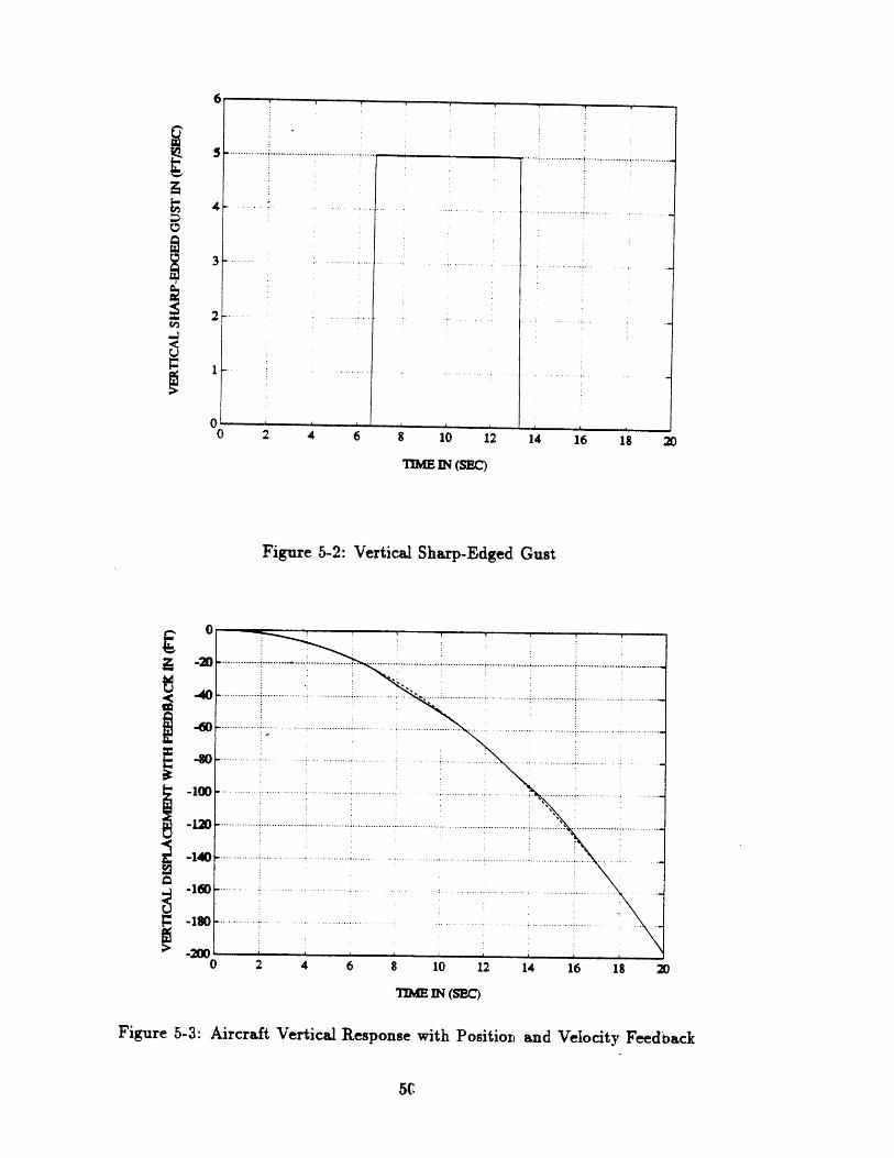
5-2 Vertical Sharp-Edged Gust ........................ 50

5-3 Aircraft Vertical Response with Position and Velocity Feedback . . . 50

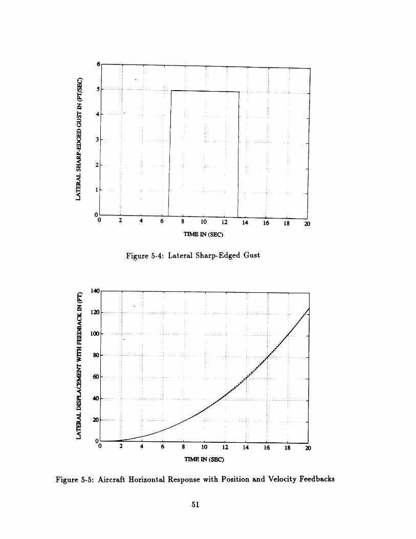
5-4 Lateral Sharp-Edged Gust ............ .... ........ 51

5-5 Aircraft Horizontal Response with Position and Velocity Feedbacks 51

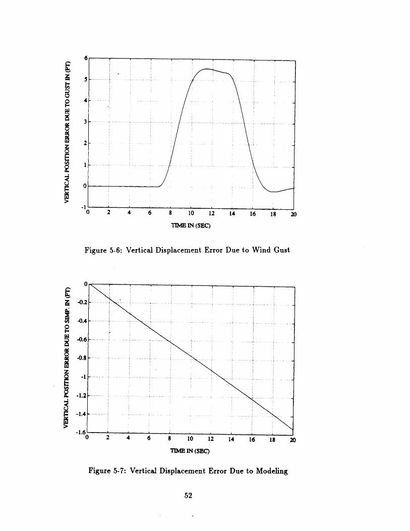
5-6 Vertical Displacement Error Due to Wind Gust . .. ..... . . . . 52

5-7 Vertical Displacement Error Due to Modeling . . . . ......... . . . . 52

5-8 Horizontal Displacement Error Due to Wind Gust ....... . . . . 53

5-9 Horizontal Displacement Error Due to Modeling . ........... 53

Chapter 1

Introduction

1.1 Concept of Optimal Trajectory Planner

As the objectives of a fighter aircraft mission increase, so does the pilot workload. In

addition to the regular navigational tasks, the pilot would be responsible for meeting

various mission requirements. He would have to insure the success of the mission by

avoiding possible ground threats en route. The geographic locations of radars have

a principal impact upon planning a "safe" flight path. Moreover, the pilot would be

required to meet time and fuel constraints simultaneously. Such constraints are im-

posed by the aircraft's fuel consumption and the possibility of mobile ground targets.

Other conceivable obstacles to overcome during the mission are natural threats like

weather conditions and terrain nature.

Severe thunderstorms may jeopardize the feasibility of a mission and its success.

They can cause significant changes in planning a minimum risk flight path and, con-

sequently, a possible exposition of the aircraft to radars or missile sites.

In general, mountain terrain demands substantially rapid maneuvering. The aircraft's

structural limits can be reached while following a steeply varying terrain. Further-

more, the pilot's ability to maneuver may deteriorate trying to avoid nearby ground

threats. In order to alleviate the pilot workload, the concept of an automatic mission

planning system was devised.

For the purpose of this research, the mission planning system can be thought to con-

Goalpoint

Planner

ThreatDatabase

IFOptimalCommands

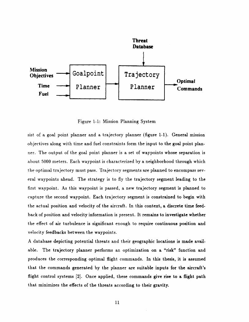
Figure 1-1: Mission Planning System

sist of a goal point planner and a trajectory planner (figure 1-1). General mission

objectives along with time and fuel constraints form the input to the goal point plan-

ner. The output of the goal point planner is a set of waypoints whose separation is

about 5000 meters. Each waypoint is characterized by a neighborhood through which

the optimal trajectory must pass. Trajectory segments are planned to encompass sev-

eral waypoints ahead. The strategy is to fly the trajectory segment leading to the

first waypoint. As this waypoint is passed, a new trajectory segment is planned to

capture the second waypoint. Each trajectory segment is constrained to begin with

the actual position and velocity of the aircraft. In this context, a discrete time feed-

back of position and velocity information is present. It remains to investigate whether

the effect of air turbulence is significant enough to require continuous position and

velocity feedbacks between the waypoints.

A database depicting potential threats and their geographic locations is made avail-

able. The trajectory planner performs an optimization on a "risk" function and

produces the corresponding optimal flight commands. In this thesis, it is assumed

that the commands generated by the planner are suitable inputs for the aircraft's

flight control systems [2]. Once applied, these commands give rise to a flight path

that minimizes the effects of the threats according to their gravity.

Trajectory

Planner

MissionObjectives

TimeFuel

I

I

1.2 Thesis Objectives

Models of the flight control systems must be embedded in the optimization process.

In previous works [1, 2], simple models of the flight control systems were used in

different optimizing algorithms to generate suitable flight commands. Clearly, the

degree of complexity in modeling the aircraft dynamics and its flight control systems

affects the optimal strategy generated by the planner. The actual trajectory flown

by the aircraft depends upon the accuracy in modeling its dynamic equations and is

altered by varying the models of the control systems.

This thesis investigates the fidelity of the flight control systems needed in the trajec-

tory planner. The disadvantage of very complex modeling of the control systems is

an increased computational burden, and hence an untimely generation of the optimal

commands. Such sluggishness may cause the aircraft to fly a trajectory leading to

radar detection or missile sites. However, oversimplified models also tend to sub-

stantially deviate the aircraft from the optimal flight path and expose it to similar

threats. Therefore, it is of interest to determine the minimum degree of complexity

of the flight control systems required by the trajectory planner.

Another issue discussed in this thesis is the monitoring of the position and velocity

of the aircraft. If such monitoring is absent between every set of two waypoints, the

actual aircraft trajectory will be directly affected by wind shears and discrete gusts.

Determination of the need for position and velocity feedbacks is predicated on the

aircraft responses to such disturbances.

1.3 Thesis Organization

Towards the goal of achieving the previous objectives, chapter 2 discusses the designs

of the flight control systems using full aircraft dynamics. Motives for dealing with

full dynamics are presented. Performance limits and response characteristics of the

control systems are studied and evaluated. In chapter 3, the effects of stochastic

wind disturbances are addressed. The aircraft responses to wind gusts characterized

by their Dryden spectra are determined. Deterministic models of wind gusts are

described in chapter 4. The question of continuous monitoring of position and velocity

is also addressed. Command updates based on position and velocity feedbacks and

the resulting aircraft responses are discussed in chapter 5. Flight path errors due

to wind disturbances and model simplification are examined. The required degree

of complexity in the models of the control systems is also presented. Finally, the

results are summarized in chapter 6. Also presented there, are recommendations and

directions for further research.

m

Chapter 2

Flight Control Systems Designs

2.1 Usage of Full Aircraft Dynamics

The objective of this thesis is to determine how complex the models of the flight

control systems in the optimal trajectory planner need to be. Having this in mind, it

is important to investigate the ability of the aircraft to follow the optimal trajectory.

If the flight control systems are not well modeled, the actual aircraft trajectory will

deviate from that predicted by the planner. The susceptibility of the airplane to be

detected by radar will increase and render the mission more dangerous and harder to

accomplish.

On the other hand, increasing the complexity of the models of the flight control

systems may prevent the trajectory planner from converging to the optimal commands

on time. That is, after one waypoint is passed, commands to steer the aircraft to the

next waypoint, while minimizing a certain risk function, may not be available. When

the aircraft is flying over a rough terrain with steep hills or narrow valleys, the timely

availability of the flight commands will be crucial to the success of the mission.

Using full aircraft dynamics will enable us to compare complex versus simplified

models. Subsequently, we can determine the least complex the flight control systems

need to be based on the aircraft responses to commands and wind disturbances.

Another motive to deal with full aircraft dynamics is the determination of the need

for continuous monitoring of position and velocity. Wind gusts and wind shears are

m

widespread in the atmosphere. They form the major source of disturbances which

produce significant trajectory deviations. Since the aircraft in this research is assumed

to be flying at 200 feet above the ground, deviations of 25 feet or larger are of concern

and would necessitate that position and velocity be monitored continuously. As will

be seen later, position and velocity feedbacks proved to be necessary.

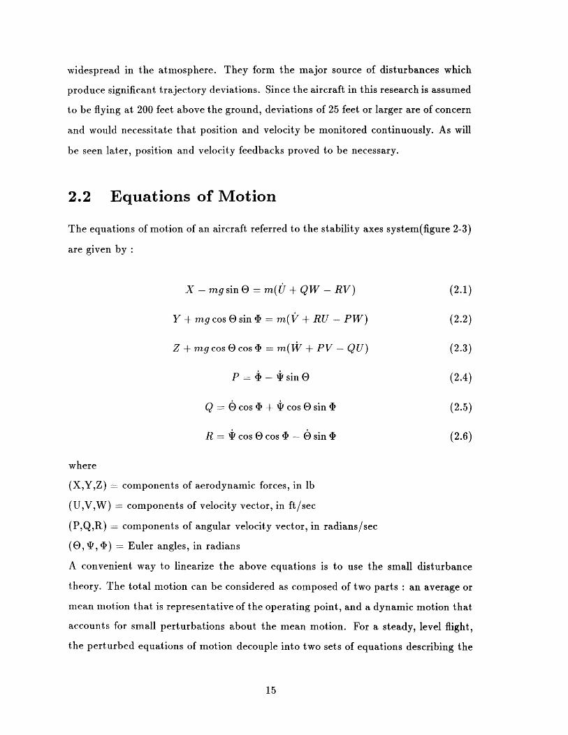
2.2 Equations of Motion

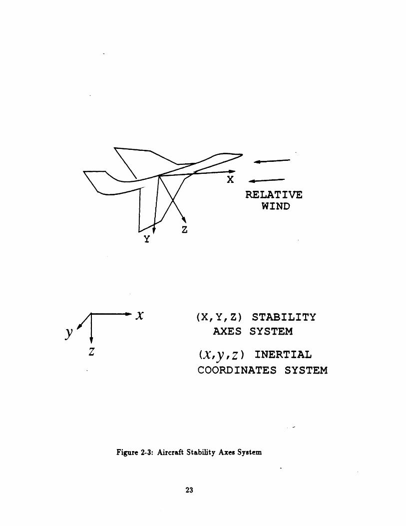
The equations of motion of an aircraft referred to the stability axes system(figure 2-3)

are given by :

X - mg sin 0 = m(U + QW - RV) (2.1)

Y + mg cos O sin 4 = m(V + RU - PW) (2.2)

Z + mg cos O cos 4 = m(W + PV - QU) (2.3)

P = - -ý sin O (2.4)

Q = O cos (b + 9 cos 0 sin 4 (2.5)

R = T cos O cos 4 - O sin 4 (2.6)

where

(X,Y,Z) = components of aerodynamic forces, in lb

(U,V,W) = components of velocity vector, in ft/sec

(P,Q,R) = components of angular velocity vector, in radians/sec

(O, •I, ) = Euler angles, in radians

A convenient way to linearize the above equations is to use the small disturbance

theory. The total motion can be considered as composed of two parts : an average or

mean motion that is representative of the operating point, and a dynamic motion that

accounts for small perturbations about the mean motion. For a steady, level flight,

the perturbed equations of motion decouple into two sets of equations describing the

longitudinal and the lateral motions of the aircraft. This decoupling property aids in

designing the longitudinal and the lateral flight control systems independently.

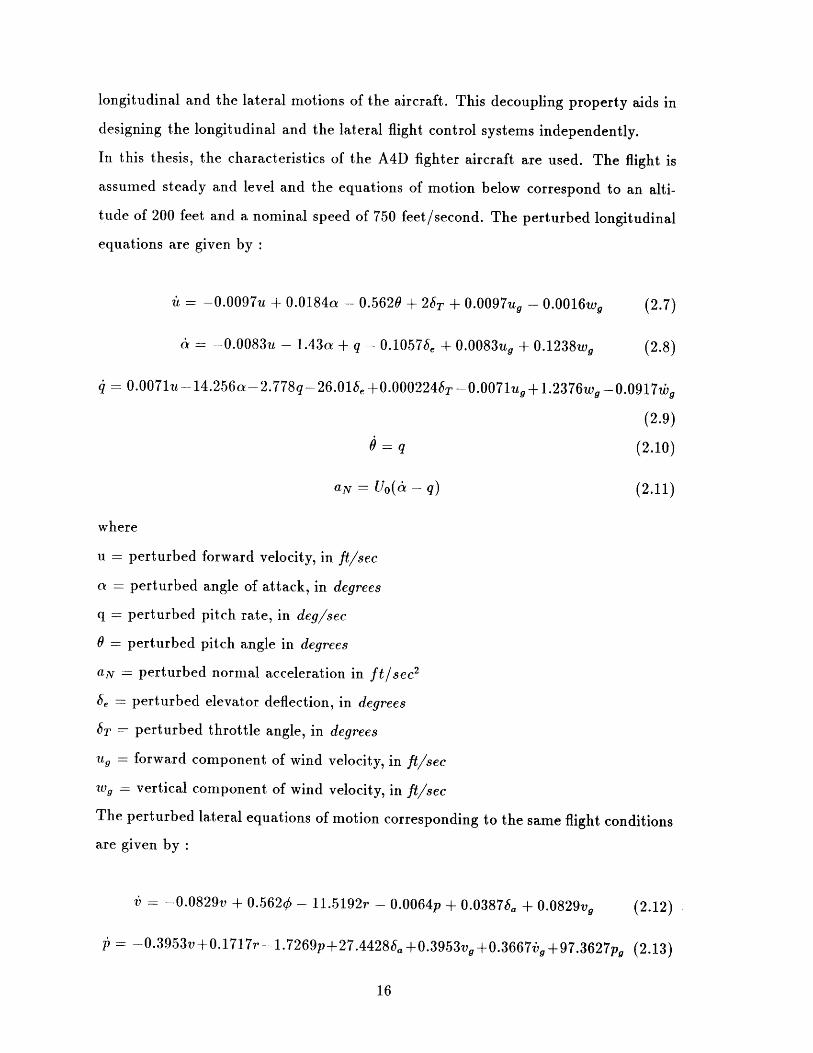
In this thesis, the characteristics of the A4D fighter aircraft are used. The flight is

assumed steady and level and the equations of motion below correspond to an alti-

tude of 200 feet and a nominal speed of 750 feet/second. The perturbed longitudinal

equations are given by :

it = -0.0097u + 0.0184a - 0.5620 + 26T + 0.0097ug - 0.0016 wg (2.7)

a = -0.0083u - 1.43a + q - 0.10576& + 0.008 3ug + 0.1238wg (2.8)

= 0.0071u- 14 .256a-2.778q- 26.016S +0.000 2 2 4 5T-0.0071ug + 1.2376wg -0.0 9 17tbg

(2.9)

0 =q (2.10)

aN = Uo(& - q) (2.11)

where

u = perturbed forward velocity, in ft/sec

a = perturbed angle of attack, in degrees

q = perturbed pitch rate, in deg/sec

0 = perturbed pitch angle in degrees

aN = perturbed normal acceleration in ft/sec2

S, = perturbed elevator deflection, in degrees

5T = perturbed throttle angle, in degrees1g = forward component of wind velocity, in ft/sec

wg = vertical component of wind velocity, in ft/sec

The perturbed lateral equations of motion corresponding to the same flight conditions

are given by :

i, = -0.0829v + 0.5620 - 11.5192r - 0.00 64p + 0.03876a + 0.0 82 9 vg (2.12)

p = -0.3953v+0.1717r- 1.7 2 69p+ 2 7 .4 4 2 86 a +0.3953v +0.3667ib• + 9 7.3 6 2 7pg (2.13)

II

÷ = 0.2922v - 0.0893r - 0.2922v, + 0. 0 0 8 3· bg + 3 .7 4 7 1pg,

¢=-p (2.15)

where

v = perturbed side velocity, in ft/sec

p = perturbed roll rate, in deg/sec

r = perturbed yaw rate, in deg/sec

= roll angle, in degrees

Sa = aileron deflection, in degrees

Vg = lateral component of wind velocity, in ft/sec

p, = roll due to gradient of vertical component of wind velocity along the span of the

aircraft, in 1/sec

Since the aircraft is inherently stable in yaw, the coordination between the aileron

deflection, 6a, and the rudder deflection, 6,, was chosen to cancel out the effect of the

aileron and the roll rate, p, on the yaw rate, r. In this case, the rudder deflection is

given by :

6, - -0.048p + 0.28956a (2.16)

The longitudinal and the lateral equations of motion are referred to the stability axes

system of the aircraft (figure 2-3). This axes system moves with the aircraft. It

consists of the x-axis pointing in the relative wind direction. The y-axis points along

the right wing of the aircraft. The direction of the z-axis is given by the following

cross product : 1, = l. x ly, where l4 and l, are the unit vectors along the x and y

axes respectively. The z-axis is positive down in level flights

Because of the decoupling property, it is possible to design the longitudinal and the

lateral flight control systems independently. The decoupling applies to level flights

(i.e. (0o = 0). However, even for large nominal values of the roll angle, (+4o = O(7r/2)),the designed flight control systems were insensitive to the nominal value of the roll

m

II

(2.14)

angle. In this context, the equations of motion were linearized about a nonzero

nominal value of the roll angle and the control law designed for 4•0 = 0 was applied.

It was found that the locations of the closed loop poles were the same as those of

the closed loop poles corresponding to a linearization about the level flight condition.

Therefore, it is safe to state that the flight control systems designed about 4Io = 0

will lead to stable control systems for arbitrary roll angle values.

2.3 Design of Flight Control Systems

2.3.1 Longitudinal Case

According to the conclusions drawn in the previous section, the command following

loop design of the longitudinal flight control system was performed independently

from the lateral one. Several motion variables are candidates for the command input

such as the pitch angle, 0, or the flight path angle, 7 = a - 0. However, based on

the results of previous works, the normal acceleration, aN, was determined to be the

most suitable [1, 2].

In the flight control system design, the elevator deflection, e6,, and the throttle angle,

6•, were selected as the control variables. In addition to the normal acceleration, aN,T

the forward velocity, uc, was also chosen as a command variable. The availability of

the throttle deflection as a command variable offers the advantage of a concurrent

thrust control system design.

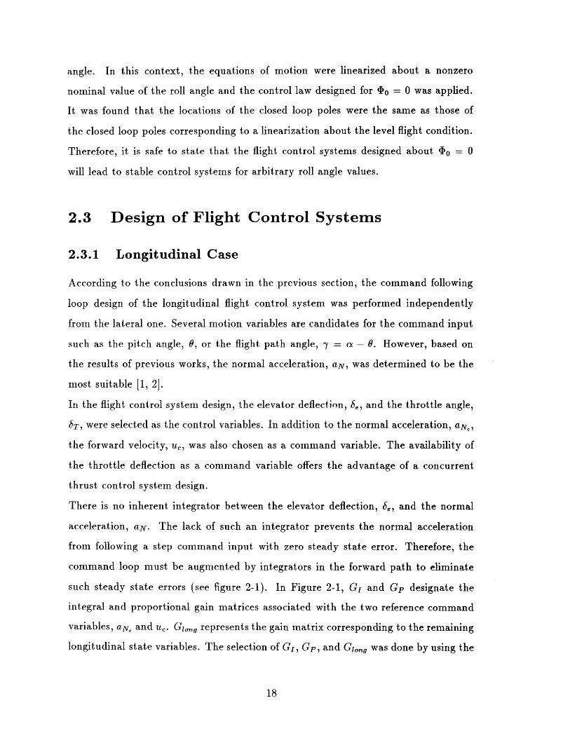
There is no inherent integrator between the elevator deflection, 5e, and the normal

acceleration, aN. The lack of such an integrator prevents the normal acceleration

from following a step command input with zero steady state error. Therefore, the

command loop must be augmented by integrators in the forward path to eliminate

such steady state errors (see figure 2-1). In Figure 2-1, G1 and Gp designate the

integral and proportional gain matrices associated with the two reference command

variables, a.N, and uc. Giong represents the gain matrix corresponding to the remaining

longitudinal state variables. The selection of GI, Gp, and Glong was done by using the

|

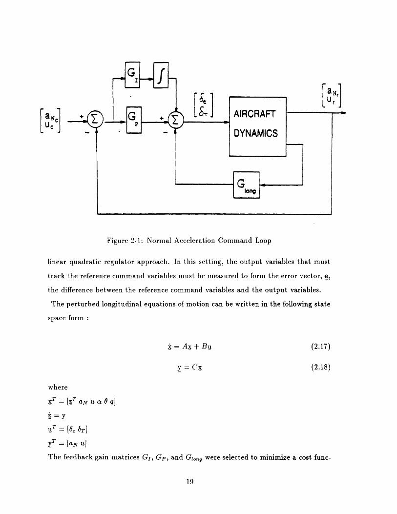
Figure 2-1: Normal Acceleration Command Loop

linear quadratic regulator approach. In this setting, the output variables that must

track the reference command variables must be measured to form the error vector, e,

the difference between the reference command variables and the output variables.

The perturbed longitudinal equations of motion can be written in the following state

space form :

_c = Ax + Bu (2.17)

y = Ox (2.18)

where

xT = [zT aN u a 0 q]

S= y

uT = [6e 6T]

yT = [aN u]

The feedback gain matrices GI, Gp, and Glong were selected to minimize a cost func-

aNcUc

I

tion of the form :

J = [xTQx + uTRu]dt (2.19)

Q and R are diagonal, penalty matrices. Their entries were picked to obtain an ac-

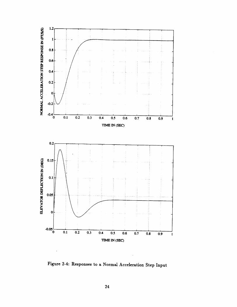
ceptable normal acceleration step response. For instance, the normal acceleration step

response is characterized by an undershoot. This undershoot is the result of a non-

minimum phase zero present in the transfer function having the elevator deflection,

56, as the input, and the normal acceleration, aN, as the output. If the percentage of

the undershoot to a step input was unacceptable, (i.e. greater than 20%), the eleva-

tor deflection would be more heavily penalized. Similarly, if the response error or the

settling time to a normal acceleration step input were too large, the penalty on the

normal acceleration state variable would be increased. The response characteristics

to a step input in the normal acceleration command are shown in figure 2-4.

2.3.2 Performance Limits

The presence of a non-minimum phase zero in the normal acceleration command

loop sets inherent performance limits in the design process. Such a limitation can

be seen by analyzing the sensitivity function. If the control system is described in a

state space form, see equations ( 2.17) and ( 2.18), the sensitivity function, S(jw) =

(I + C(jwl - A)- 1 B) - 1, describes the effect of external disturbances on the output,

y. In general, the energy content of the external disturbances is concentrated in low

frequency ranges. The aircraft is affected most by the long wavelength components

of air turbulence. To minimize the effect of wind gusts on the tracking variable,

aN, the magnitude of S(jw) must be small over the bandwidth of the system (i.e.

SS(jw)l| << 1 at low frequencies).

However, the magnitude of the sensitivity function cannot be made arbitrarily small

due to the presence of the non-minimum phase zero. In fact, the magnitude of the

sensitivity function at the frequency of the non-minimum phase zero is 1.

Using the concept of subharmonic functions [6], quantitative limits on the sensi-

tivity function can be established.

If ao designates the frequency of the non-minimum phase zero and if log | S(jw)JJ |-M for I w I< WB, then the sensitivity function will be constrained to :

log sup I S(jw)1 > M (2.20)wE- 7"r - 0

This result can be attributed to the fact that log &[S(jw)] is a subharmonic func-

tion. & designates the maximum singular value. In equation ( 2.20), M is an

arbitrary constant describing the effect of disturbance rejection. 0 is given by :

0 = 2arctan(wB/co). Unless WB < co0, the sensitivity function will be character-

ized by a substantial peak.

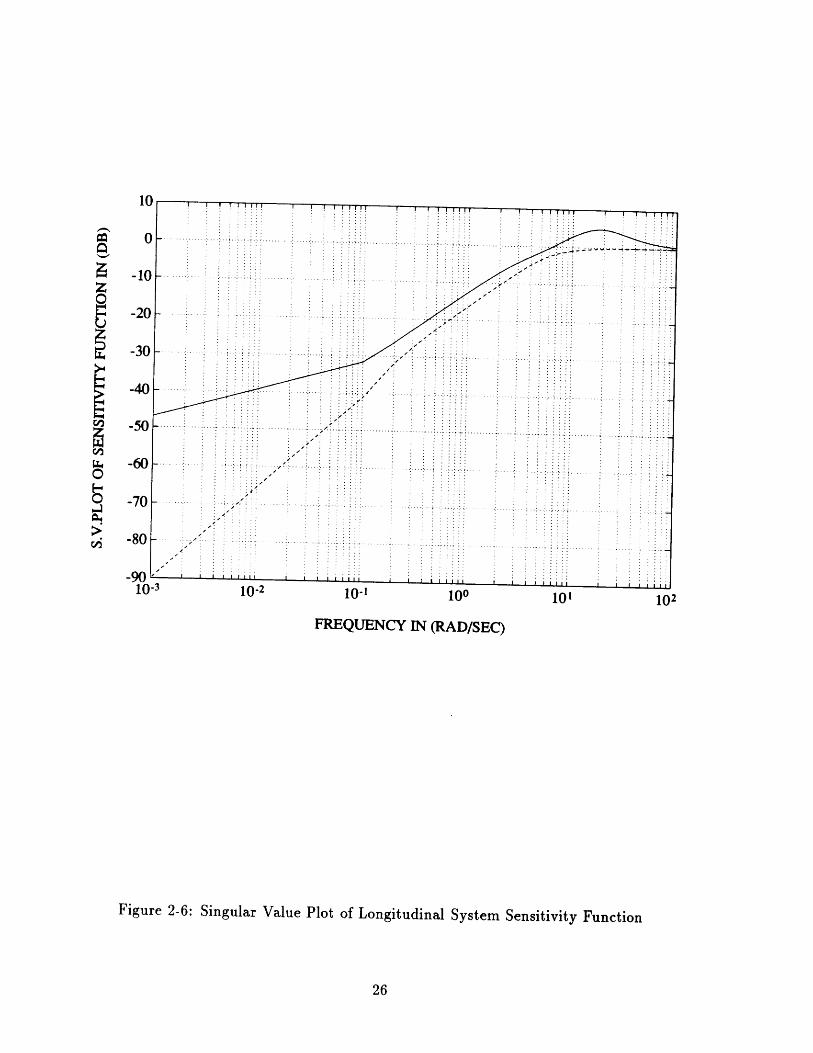
Figure ( 2-6) clearly depicts the same attribute. The normal acceleration command

loop has a non-minimum phase zero at a frequency of or0 = 19rad/sec. If the mag-

nitude of the sensitivity is decreased in the low frequency range, the severity of the

peak at higher frequencies will be more pronounced.

Another performance limit is imposed by the physical limits of the elevator. It is

necessary to maintain the elevator deflection below 250 to avoid stall characteristics

at the elevator. As a consequence, the normal acceleration response cannot track

the reference command arbitrarily fast, leading to limits on the response time of the

normal acceleration.

2.3.3 Lateral Case

The roll angle command following loop is shown in figure 2-2. The aileron deflection,

ba, was selected as the control variable. The coordination between aileron and rudder

deflections is according to equation ( 2.16). The scalar gain, g, is the proportional gain

associated with the roll angle. Giat, a gain matrix, is associated with the remaining

lateral state variables, i.e. the side velocity, v, the roll rate, p, and the yaw rate,r. Both gains, g and Giat, were evaluated by using the linear quadratic approach.

Figure 2-2: Roll Angle Command Following Loop

A quadratic cost form similar to the one used in the longitudinal loop design was

minimized; and the corresponding feedback gains were chosen to lead to an acceptable

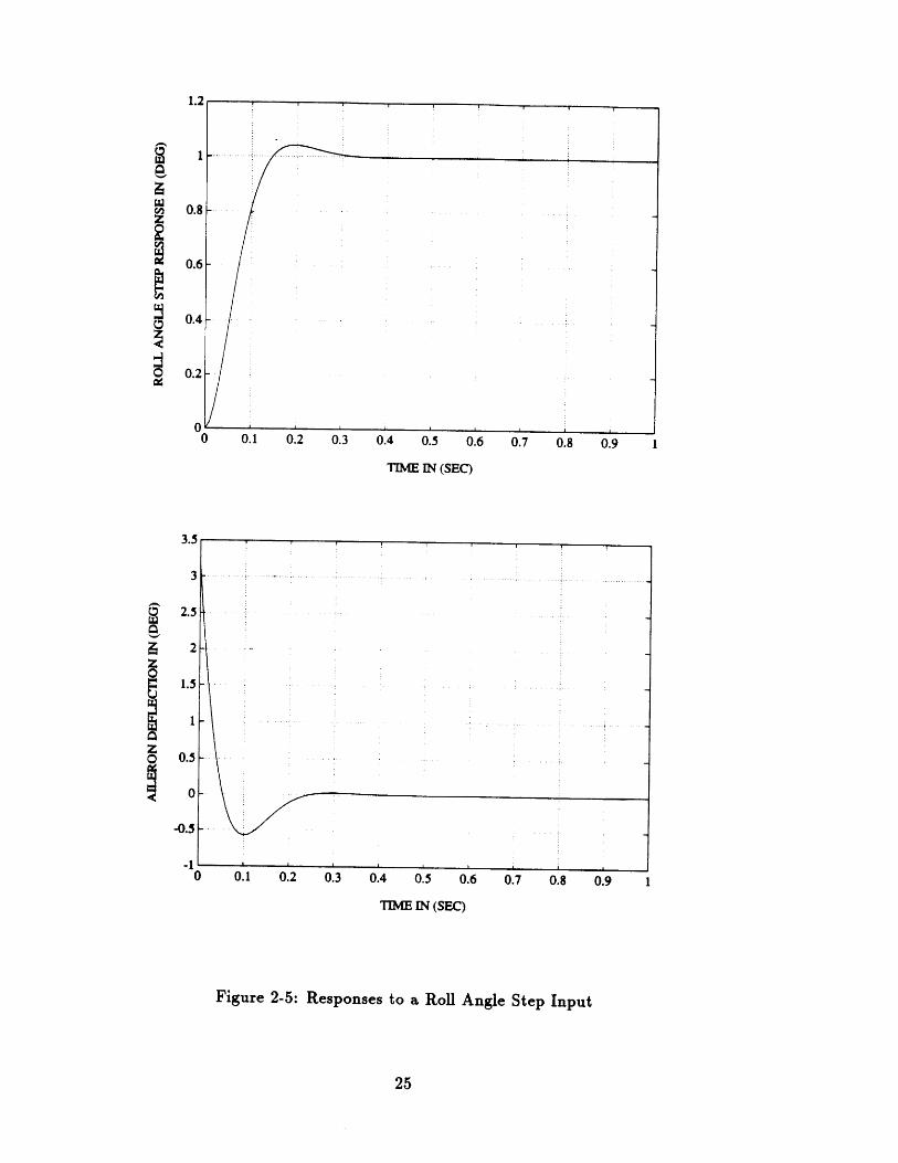
settling time in the roll angle response to a reference step input. Because of the

presence of inherent integrators in the forward loop, no artificial augmentation is

needed. The aircraft's response and the aileron deflection resulting from a roll angle

step command are shown in figures 2-5.

Although no non-minimum phase zero is present in the roll angle command loop,

performance limits exist. They are attributed to the physical constraints imposed

by the aileron deflection. Such constraints are similar to those associated with the

elevator deflection, and they prevent the roll angle from tracking a step command

input arbitrarily fast. In addition, complete rejection of arbitrarily large output

disturbances over the bandwidth of the system cannot be achieved because of these

physical constraints.

C

I

RELATIVE

RELAT IVEWIND

STABILITYAXES SYSTEM

(XyZ) INERTIALCOORDINATES SYSTEM

Figure 2-3: Aircraft Stability Axes System

(X, Y, Z)

U U.i 0.2 0.3 0.4 0.5 0.6 0.7 0.8 0.9

TIME IN (SEC)

V U.l U.2 0.3 0.4 0.5 0.6 0.7 0.8 0.9

TIME IN (SEC)

Figure 2-4: Responses to a Normal Acceleration Step Input

g

od0zPUIz

zIH1

I

m

A

1

0 0.1 0.2 0.3 0.4 0.5 0.6 0.7 0.8TIME IN (SEC)

U.1 0.2 0.3 04 05 06 07 08

TIME IN (SEC)

Figure 2-5: Responses to a Roll Angle Step Input

, 0.8

0.6

0.4

o 0.2

0

z

CI

0z8

1

0.9 1

0.9 1

m

I.V-

FREQUENCY IN (RAD/SEC)

Figure 2-6: Singular Value Plot of Longitudinal System Sensitivity Function

z

I

g8LLC

U

Chapter 3

Stochastic Analysis

If the atmosphere were uniform and wind disturbances were non existent, the de-

signed flight control systems would be satisfactory. No further augmentation to the

command loops would be needed; and the aircraft would closely follow the optimal

trajectory. However, it is known that the atmosphere is in constant motion. Gradi-

ents in temperature, pressure, and velocity give rise to air turbulence.

Since the aircraft is flying very close to the ground, the most serious effects of wind

disturbances are those that cause the aircraft to lose lift and altitude. Of equal im-

portance are the wind disturbances that lead to significant lateral deviations from the

minimum risk flight path produced by the planner.

3.1 Atmospheric Turbulence Assumptions

In this thesis, air turbulence is assumed to take the form of individual patches charac-

terized by their intensity. The intensity in each patch describes the root mean square

of any of the turbulent velocity components. The spectrum or the frequency content

of the turbulence in each patch is related to the intensity.

Another assumption often made about air turbulence is that of isotropy. Statistical

properties are assumed to be independent of orientation of axes. At low altitudes, it

is proved that the atmosphere is anisotropic. Lack of isotropy at low altitudes im-

plies that the statistical properties of the turbulence differ among the three turbulent

velocity components (ug, Vg, Wg). Furthermore, the absence of isotropy leads to the

existence of statistical cross correlations among the three velocity components. For

simplicity however, it is assumed that these cross correlations are negligible.

Taylor's hypothesis is also assumed in this thesis. The hypothesis states that time

variations are statistically equivalent to distance variations in traversing the turbu-

lence field. In this case, the temporal frequency sensed by the aircraft can be related

to the spatial frequency of the turbulence according to the following equation :

w = VQ (3.1)

where w is the temporal frequency in rad/sec, V is the aircraft's velocity in feet/sec

through the turbulence field, and Q is the spatial frequency of the air turbulence

waves in rad/feet.

Another implication of Taylor's hypothesis is that turbulence-induced aircraft re-

sponses result only from the motion of the aircraft relative to the turbulence field. In

this case, statistical properties of the turbulence as sensed by the aircraft are indepen-

dent of time. Consequently, stationary statistical methods can be used in analysis.

In this thesis, the results of wind disturbance analysis apply only to the long wave-

length components of air turbulence. The wavelengths were assumed to be at least

as large as eight times the length of the aircraft. As a consequence, the variation

of the wind gust velocity along the length or the span of the aircraft is approxi-

mately linear. To account for the effects of short wavelength turbulence, equivalent

aerodynamic force and moment terms must be calculated empirically.

3.2 Dryden Gust Spectra

There are two models that describe the spectra of air turbulence. They are known

as the von Karman and Dryden spectra. Both of these models satisfy all the math-

ematical requirements for isotropy. Although the von Karman spectra describe air

turbulence behavior more accurately, the Dryden gust spectra were analyzed in this

research. The selection of the Dryden gust spectra was based upon their rational

form; leading to significant simplification in analysis and computation. The gust

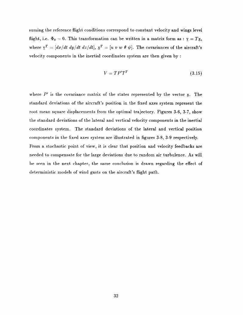
spectra associated with the three wind velocity components (ug, Vg, Wg) are given by

the following equations :

2L/ 14 (W) = 22L 1 (3.2)S Uo [1 + (L,w/Uo)2]

2LL 1 + 3(L,w/Uo) 2

v Uo [1 + (L,w/Uo) 2 ]2

2 L, 1 + 3(Lw/U) 2 (34)4Wg(W)= e (3.4)SUo [1 + (Lw/UUo) 2]2

Equations ( 3.2, 3.3, 3.4) describe the gust spectra directly in terms of the temporal

frequency, w, as sensed by the aircraft. In these equations, Uo designates the nom-

inal velocity of the aircraft, 750 ft/sec. ai, (i = ug, v, wg), represents the intensity

associated with the corresponding gust. Li (i = u,v,w) are scale lengths related to

the altitude of the aircraft and the severity of air turbulence (e.g. clear air turbu-

lence or thunderstorm turbulence). Equations ( 3.2, 3.3, 3.4) are defined such that

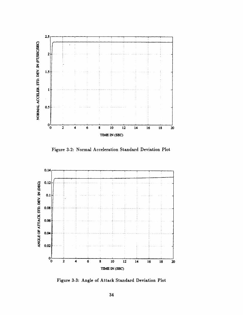
2 = f- fo i((w)dw. In the stochastic simulation, a gust intensity of 5 feet/sec was

used. It was felt that air turbulence having such intensity is not uncommon at the

aircraft's nominal altitude, 200 feet. In fact, the probability of equaling or exceeding

a 5 feet/sec intensity at 200 feet is 0.08 [4]. Clear air turbulence was also assumed in

the simulation.

Gust velocity gradients along the span of the aircraft produce substantial rolling mo-

tions. The spectrum associated with the variations of w, along the span of the aircraft

is given by :

4r / 0.+,(w) = ( )1/ (3.5)

w 4b UoLW [1 + (4bw/7rUo) 2]

where b is the aircraft wing span.

3.3 Propagation of State Covariances

The method of stochastically simulating air turbulence was to pass a Gaussian white

noise through a filter (see figure 3-1). The filter shapes the random output such that

it has certain statistical properties characteristic of the atmospheric turbulence to be

simulated. The two statistical parameters which are reproduced are the turbulence

intensity, cri, and the frequency content, 44i, through the turbulence energy spectrum.

The random effect of air turbulence on the aircraft can be evaluated by propagating

the covariances of the state variables of interest in time. In general, a stochastic pro-

cess can be described by a linear differential equation driven by white noise so that

the power spectral density of the response is the same as the power spectral density

of the original stochastic process.

It is of interest to examine the aircraft stochastic response after implementing the de-

signs of the flight control systems. The aircraft equations of motion can be combined

with the differential equations corresponding to the shaping filters. The resulting

equations can be conveniently arranged in the following state space form :

k = Ax + Bw (3.6)

y = x (3.7)

where the correlation of w is : E[w(t)wT (t - r)] = IS(r). Since equation( 3.6) is

driven by white noise, the propagation of the state covariances is given by the matrix

Lyapunov equation :

P = AP + PAT + BBT (3.8)

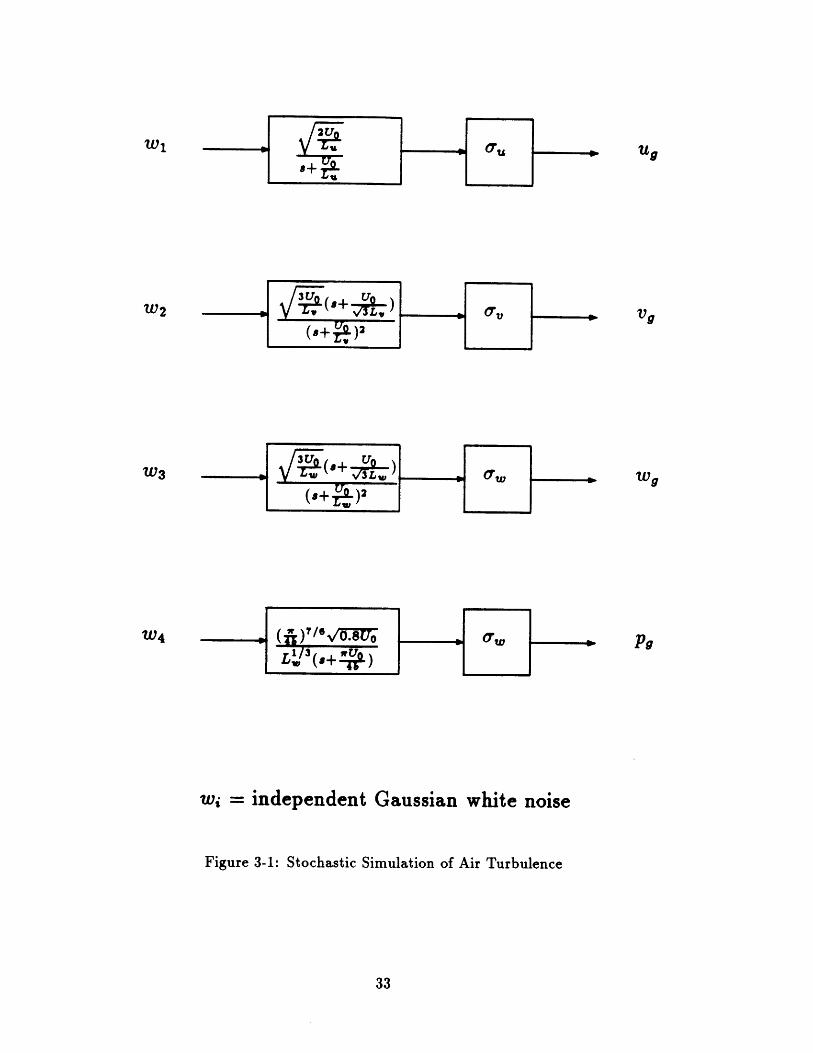
where P represents the state covariance matrix. Integrating equation( 3.8) forward in

time with zero initial conditions (i.e. P(0) = 0), the variations of the state covariances

with respect to time can be determined. Figure 3-2 shows how the standard deviation

of the normal acceleration evolves with time. Similar standard deviation plots for the

angle of attack, the roll angle, and the side velocity are shown in figures 3-3, 3-4, 3-5

respectively.

To appreciate the effect of the random wind turbulence on the aircraft trajectory,

standard deviations of the aircraft's position and velocity seen in a fixed axes system

should be evaluated. Towards this goal, a transformation between the aircraft's sta-

bility axes system and the inertial system must be performed. The components of

the aircraft's velocity in the fixed axes system are given by :

dX/dt = U cos - cos T + V(sin 4 sin 0 cos 9 - cos 4 sin 9) +

W(cos 'b sin 0 cos T + sin 1D sin ') (3.9)

dY/dt = U cos 0 sin I + V(sin 4 sin 0 sin T + cos t cos T) +

W(cos ¶J sin 0 sin T - sin (b cos T) (3.10)

dZ/dt = -U sin + V sin 4cos + W coscoscos (3.11)

Perturbing the motion variables about their nominal values (i.e. U = Uo+u, 0 = 0o0+

etc.), and neglecting second and higher order terms, the perturbed inertial compo-

nents of the aircraft's velocity are obtained :

dz/dt = (Uo + u)cos00 - UoOsinOo + wsin00 (3.12)

dy/dt = Uo cos00 + v (3.13)

dz/dt = -(Uo + u)sin 00 - UoO cos o0 + wcos0o (3.14)

The above equations, describing the transformation sought after, were arrived at as-

suming the reference flight conditions correspond to constant velocity and wings level

flight, i.e. 0o = 0. This transformation can be written in a matrix form as : v = Tx,

where vT = [dx/dt dy/dt dz/dt], xT = [u v w 0 0]. The covariances of the aircraft's

velocity components in the inertial coordinates system are then given by :

V = TP'TT (3.15)

where P' is the covariance matrix of the states represented by the vector x. The

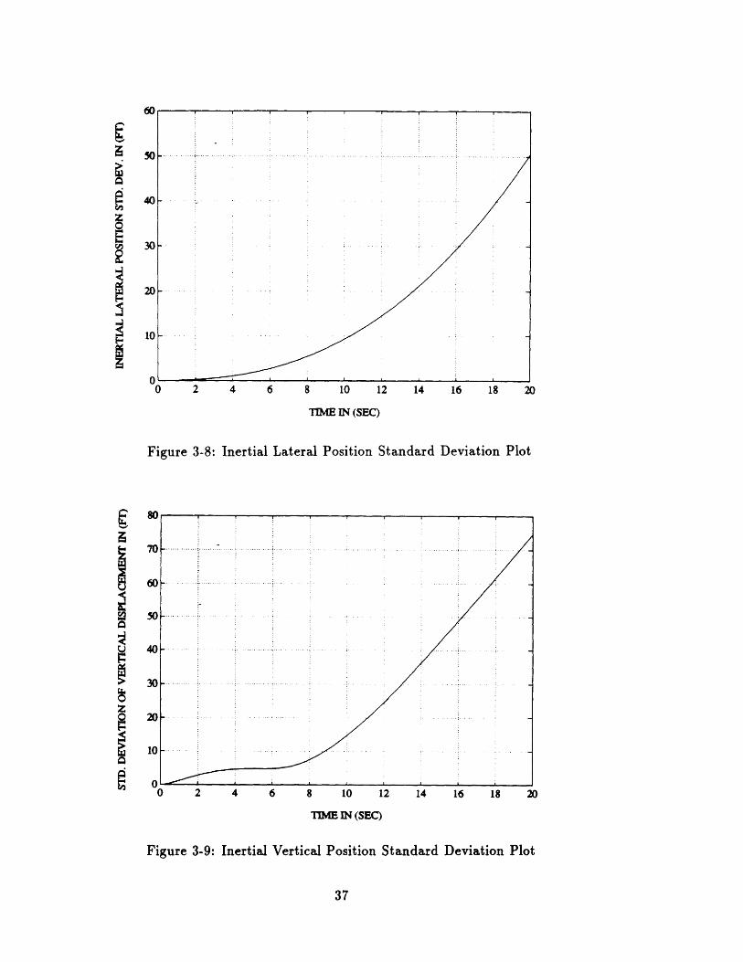
standard deviations of the aircraft's position in the fixed axes system represent the

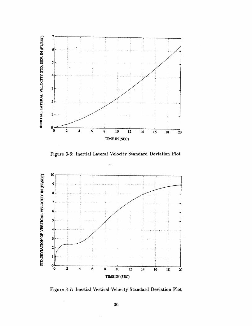
root mean square displacements from the optimal trajectory. Figures 3-6, 3-7, show

the standard deviations of the lateral and vertical velocity components in the inertial

coordinates system. The standard deviations of the lateral and vertical position

components in the fixed axes system are illustrated in figures 3-8, 3-9 respectively.

From a stochastic point of view, it is clear that position and velocity feedbacks are

needed to compensate for the large deviations due to random air turbulence. As will

be seen in the next chapter, the same conclusion is drawn regarding the effect of

deterministic models of wind gusts on the aircraft's flight path.

U

W2

W3

W4

wi = independent Gaussian white noise

Figure 3-1: Stochastic Simulation of Air Turbulence

Wl Ug

Vg

Wg

U

0.5

0 2 4 6 8 10 12 14 16 18 20

TIME IN (SEC)

Figure 3-2: Normal Acceleration Standard Deviation Plot

0.

0

0.1

0.4

0.1

0.(

0 2 4 6 8 10 12 14 16 18 20

TIME IN (SEC)

Figure 3-3: Angle of Attack Standard Deviation Plot

I ' I 1 I I 1 I I

1.5 ·

I

-

2 4 6 8 10 12 14 16 18 20

TIME IN (SEC)

Figure 3-4: Roll Angle Standard Deviation Plot

TIME IN (SEC)

Figure 3-5: Side Velocity Standard Deviation Plot

1% iAGUST INTENSITY = 5 FT/SEC

2 4 6 8 10 12 14 16 18 20

TIME IN (SEC)

Figure 3-7: Inertial Vertical Velocity Standard Deviation Plot

U 2 4 6 8 10 12 14 16 18 20

TIME IN (SEC)

Figure 3-6: Inertial Lateral Velocity Standard Deviation Plot

TIME IN (SEC)

Figure 3-9: Inertial Vertical Position Standard Deviation Plot

L_

0 2 4 6 8 10 12 14 16 18 20

TIME IN (SEC)

Figure 3-8: Inertial Lateral Position Standard Deviation Plot

Chapter 4

Deterministic Analysis

Meteorological circulations or terrain-induced airflows can on occasion induce large

and rapidly changing variations in air velocity over small distances. These variations

produce corresponding sudden changes in the relative flow of air over the aircraft's

wings and other lifting surfaces, with attendant changes in the aircraft's actual flight

path. In order to gain insight about the severity of ensuing trajectory deviations,

deterministic models of air turbulence were analyzed and simulated.

4.1 Sharp-Edged Gusts

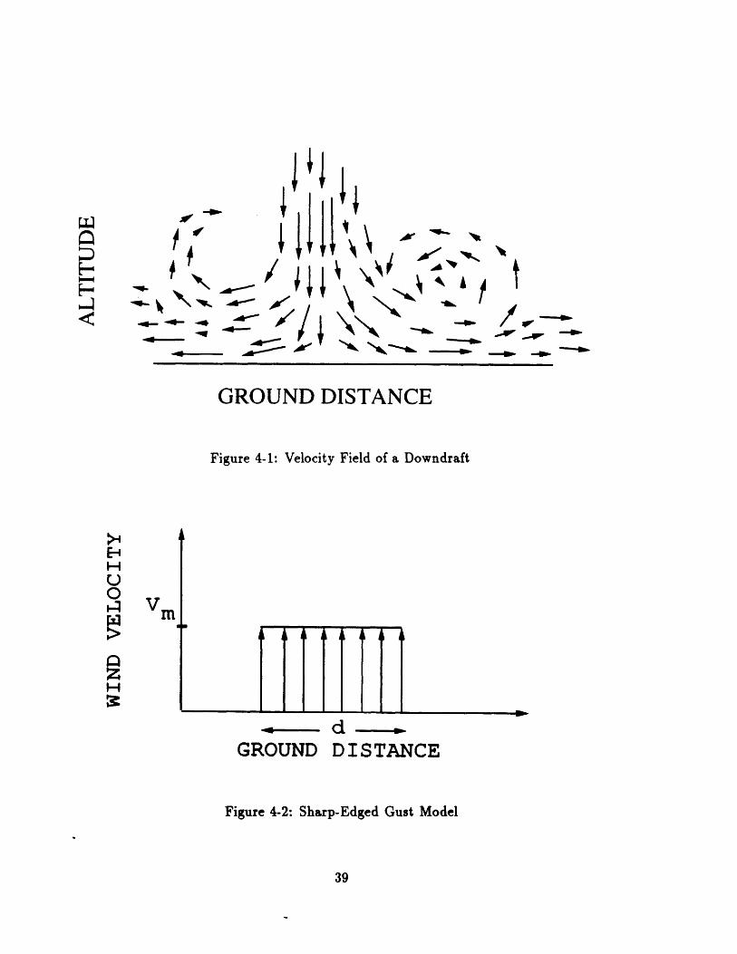
Separate air masses do not mix readily when they come into contact if they have

different temperatures and humidity. Instead, the colder, more dense air mass passes

below the warmer, less dense air mass. Consequent downdrafts result from the airflow

between the two air masses. As the downdrafts approach the ground, they turn and

move outwards along the Earth's surface. The velocity field depicting such air motion

is shown in figure 4-1.

As the aircraft traverses through the downdraft, the effect of the wind gust it senses

can be modeled as a sharp-edged gust (see figure 4-2). The time period during which

the aircraft experiences air turbulence can be varied by changing the length of the

gust, d. The intensity of the gust translates directly into the maximum amplitude,

V,,, of the velocity of the gust model.

.4 **,-V

01

A*--- '0004-Ole

___ -q1

* 4dv jQNZ*\'t

\ NZ~I/

GROUND DISTANCE

Figure 4-1: Velocity Field of a Downdraft

GROUNDdDISTANCE

Figure 4-2: Sharp-Edged Gust Model

Hr-4

r 7P_ Fýi

m lI

I !I I I a

*lr -Ift

dGROUND DISTANCE

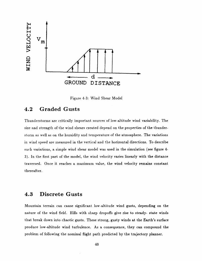
Figure 4-3: Wind Shear Model

4.2 Graded Gusts

Thunderstorms are critically important sources of low-altitude wind variability. The

size and strength of the wind shears created depend on the properties of the thunder-

storm as well as on the humidity and temperature of the atmosphere. The variations

in wind speed are measured in the vertical and the horizontal directions. To describe

such variations, a simple wind shear model was used in the simulation (see figure 4-

3). In the first part of the model, the wind velocity varies linearly with the distance

traversed. Once it reaches a maximum value, the wind velocity remains constant

thereafter.

4.3 Discrete Gusts

Mountain terrain can cause significant low-altitude wind gusts, depending on the

nature of the wind field. Hills with sharp dropoffs give rise to steady- state winds

that break down into chaotic gusts. These strong, gusty winds at the Earth's surface

produce low-altitude wind turbulence. As a consequence, they can compound the

problem of following the nominal flight path predicted by the trajectory planner.

t--4

UOv0 VmH4

>H

I

dGROUND DISTANCE

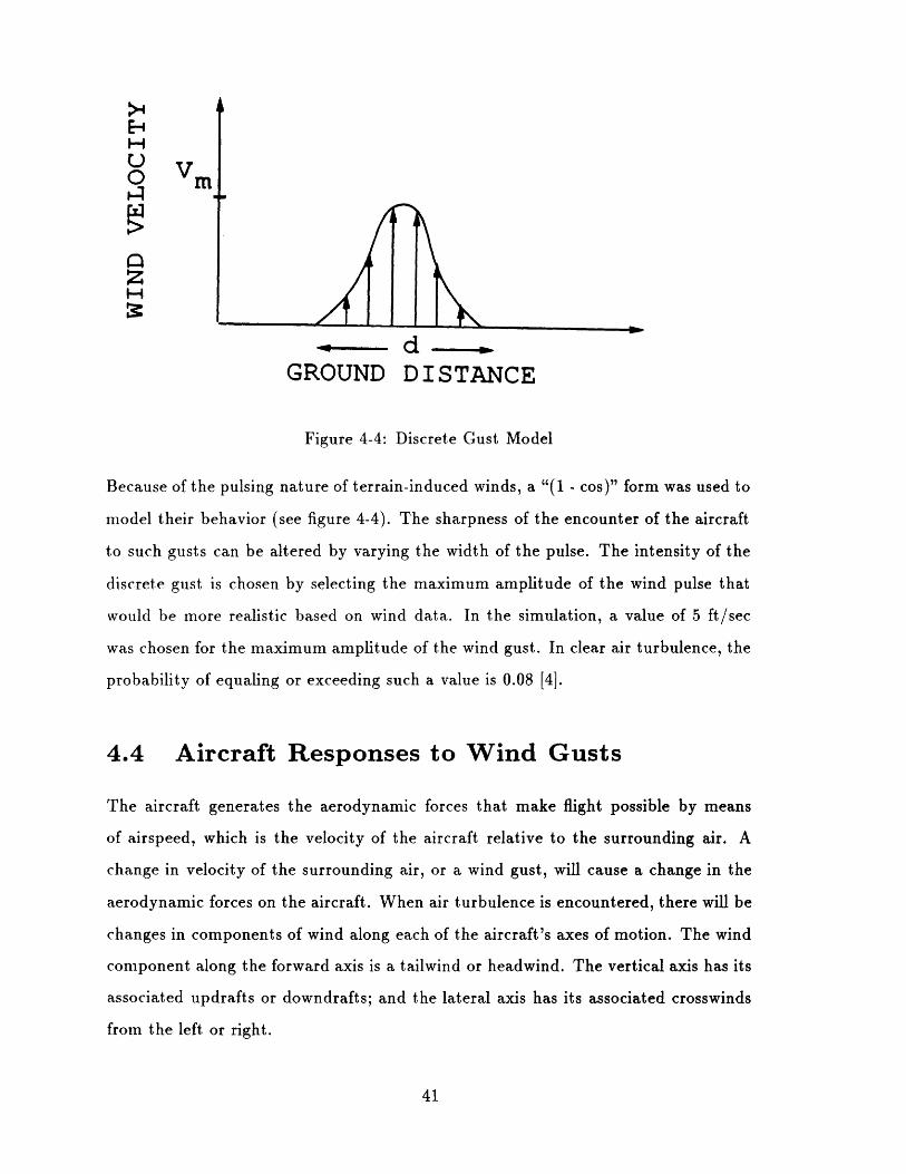
Figure 4-4: Discrete Gust Model

Because of the pulsing nature of terrain-induced winds, a "(1 - cos)" form was used to

model their behavior (see figure 4-4). The sharpness of the encounter of the aircraft

to such gusts can be altered by varying the width of the pulse. The intensity of the

discrete gust is chosen by selecting the maximum amplitude of the wind pulse that

would be more realistic based on wind data. In the simulation, a value of 5 ft/sec

was chosen for the maximum amplitude of the wind gust. In clear air turbulence, the

probability of equaling or exceeding such a value is 0.08 [4].

4.4 Aircraft Responses to Wind Gusts

The aircraft generates the aerodynamic forces that make flight possible by means

of airspeed, which is the velocity of the aircraft relative to the surrounding air. A

change in velocity of the surrounding air, or a wind gust, will cause a change in the

aerodynamic forces on the aircraft. When air turbulence is encountered, there will be

changes in components of wind along each of the aircraft's axes of motion. The wind

component along the forward axis is a tailwind or headwind. The vertical axis has its

associated updrafts or downdrafts; and the lateral axis has its associated crosswinds

from the left or right.

0 V M

Hzr

I

Each of these wind components will produce a different response based on the air-

craft's aerodynamic configuration. The effects of tailwinds or headwinds on the air-

craft trajectory are not of major concern. The reason stems from the fact that the

trajectory planner is made aware of the aircraft's position and velocity as each way-

point is passed. Any substantial loss of time can be made up by increasing the thrust

over the next sets of waypoints. Instead, vertical and lateral wind gusts are the

principal sources expected to cause significant flight deviations.

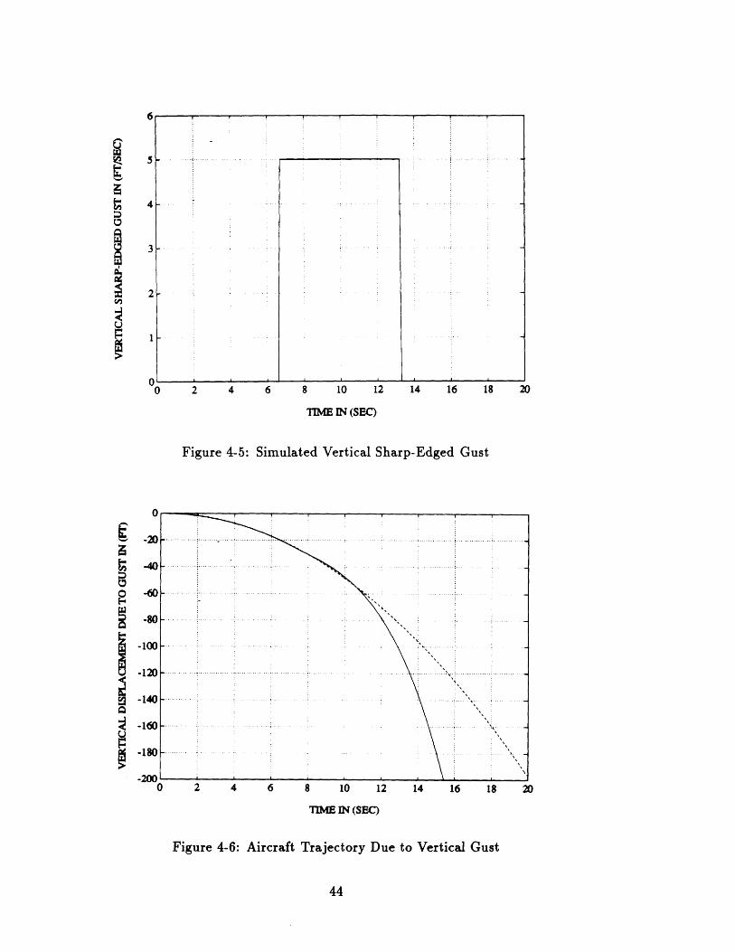
4.4.1 Response to Vertical Gusts

An updraft disturbs the airplane by increasing its angle of attack. This increased

angle of attack increases lift and drag, which cause the aircraft to climb and decelerate.

Assuming the presence of static stability, the increased lift causes the aircraft to pitch

nose-down to reduce the angle of attack and to recover its original value.

The opposite situation, a downdraft, decreases the aircraft's angle of attack, thus

reducing lift and causing it to sink. To appreciate the effect of air turbulence on the

aircraft, a vertical sharp-edged gust of 5 ft/sec intensity was simulated. Figure 4-6

shows the nominal trajectory resulting from a normal acceleration step command. In

the presence of a wind gust, it is clear that the trajectory deviations are significant

and too large to be tolerable. To remedy this problem, position and velocity feedbacks

will be needed.

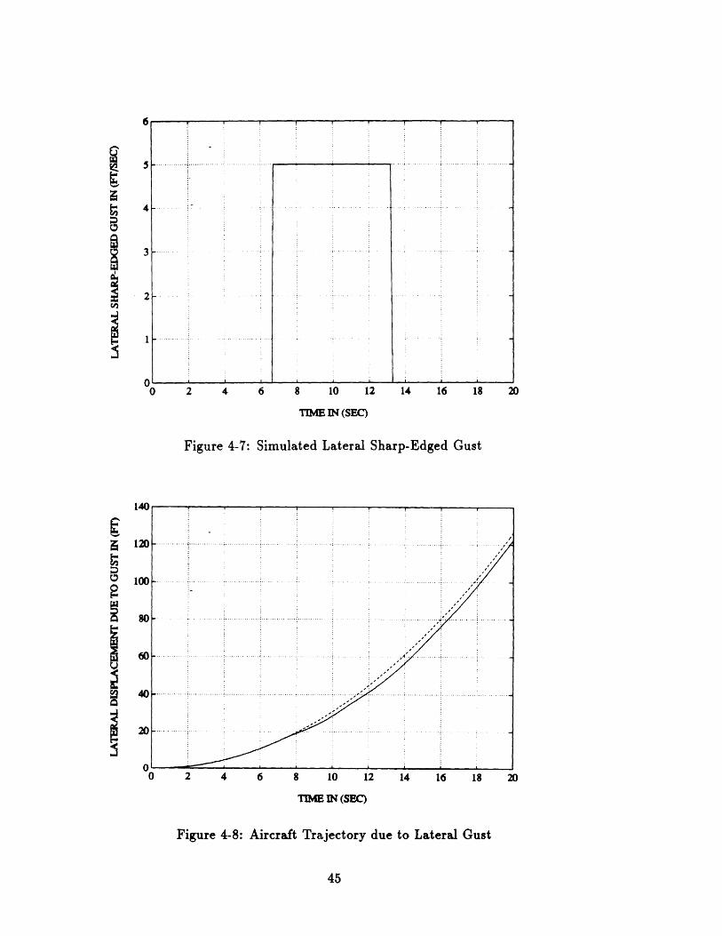
4.4.2 Response to Lateral Gusts

Crosswinds and lateral wind shears act on the aircraft by generating side forces plus

yawing and rolling moments. The initial response is to "weathervane" into the wind.

In a steady crosswind, the airplane will eventually stabilize with the wings approxi-

mately level and flying into the wind on a new heading. Basically, lateral wind shears

do not cause large changes in altitude or airspeed. However, if large bank angles de-

velop, a small loss of lift and rate of descent will be generated. Figure 4-8 shows the

effect of a lateral sharp-edged gust having a 5 ft/sec intensity. Clearly, the horizontal

displacement is not very severe. The discrepancy between the longitudinal and the

lateral responses is attributed to the different aerodynamic configurations seen by the

wind.

Observing the lateral response due to air turbulence, one might conclude that lateral

flight path corrections are not needed. However, it is known that deterministic models

of lateral wind gusts can lead to unconservative results. Instead, one should refer to

the random disturbance analysis. Stochastic results discussed in the previous chapter

determined the need for both, lateral and vertical, trajectory corrections.

0 2 4 6 8 10 12 14 16 18 20

TIME IN (SEC)

Figure 4-6: Aircraft Trajectory Due to Vertical Gust

44

_ · · 1 · ·

1 I I i I I , I I i

---

2 4 6 8 10 12 14 16 18 20

TIME IN (SEC)

Figure 4-5: Simulated Vertical Sharp-Edged Gust

0 2 4 6 8 10 12 14 16 18 20

TIME IN (SEC)

Figure 4-7: Simulated Lateral Sharp-Edged Gust

0 2 4 6 8 10 12 14 16 18 20

TIME IN (SEC)

Figure 4-8: Aircraft Trajectory due to Lateral Gust

i I i i I I

II I i i | i I i |

.... I

.i .. .. .. . .. -. . . ......

:

II

Chapter 5

Complexity of Flight Control

System Models

Results established in the two previous chapters dictate the necessity of continuous

monitoring and control of the aircraft's position and velocity. Such monitoring is

needed to closely track the commands generated by the planner in the presence of

air turbulence. In addition, a radar altitude sensor and a forward-looking radar are

unequivocally needed to avoid any imminent ground impact. This is necessary be-

cause of the expected low-altitude nature of the flight paths. The present chapter

discusses how the flight commands are updated to compensate for trajectory devia-

tions. The minimum degree of complexity of the flight control system models needed

in the trajectory planner is also presented.

5.1 Command Updates

Since position and velocity feedbacks have been proved to be indispensable, the com-

nmands to the flight control systems must incorporate information about the flight

path deviations. Between any set of two waypoints, the aircraft trajectory can be

parametrized in time after implementing the appropriate commands. Consequently,

an error vector, e, described in the inertial coordinates system can be formed. It rep-

resents the deviation between the nominal and the actual trajectories at any instant.

The command updates consist of a linear combination of the components of the air-

craft's position and velocity errors :

aN = -Kez - K2e (5.1)

= -K3e, - K4e, (5.2)

where the subscripts y and z designate respectively the lateral and vertical error com-

ponents in the stability coordinates system. The reason for including the error rate,

e, stems from the fact that it indicates future variations of the error vector, e, and

thus is helpful in stabilizing the loop. The gains, Ki, were selected by forming the

equations describing the propagation of the state variable errors and using the linear

quadratic approach. The objective was to minimize the magnitudes of the vectors e

and e. The penalty matrices were chosen to make the gains that are not associated

with the state variable errors e and e vanishingly small. The resulting flight com-

mands would then have the following form :

aN = aNn + aN (5.3)

, = n + ý (5.4)

where aN, and ,n are the nominal commands generated by the trajectory planner.

Figures 5-3 and 5-5 show the aircraft's trajectory resulting from position and velocity

feedbacks. It is assumed that the nominal commands are step functions and that a

sharp-edged gust is present en route.

Comparing figures 5-3 and 5-5 to figures 4-6 and 4-8 where position and velocity

feedbacks are absent, one can conclude that the command updates successfully re-

solved the problem of experiencing substantial deviations from the flight path that is

predicted by the planner.

aNc 1 aNr1+0.1s

Oc 1 Oer1+0.18

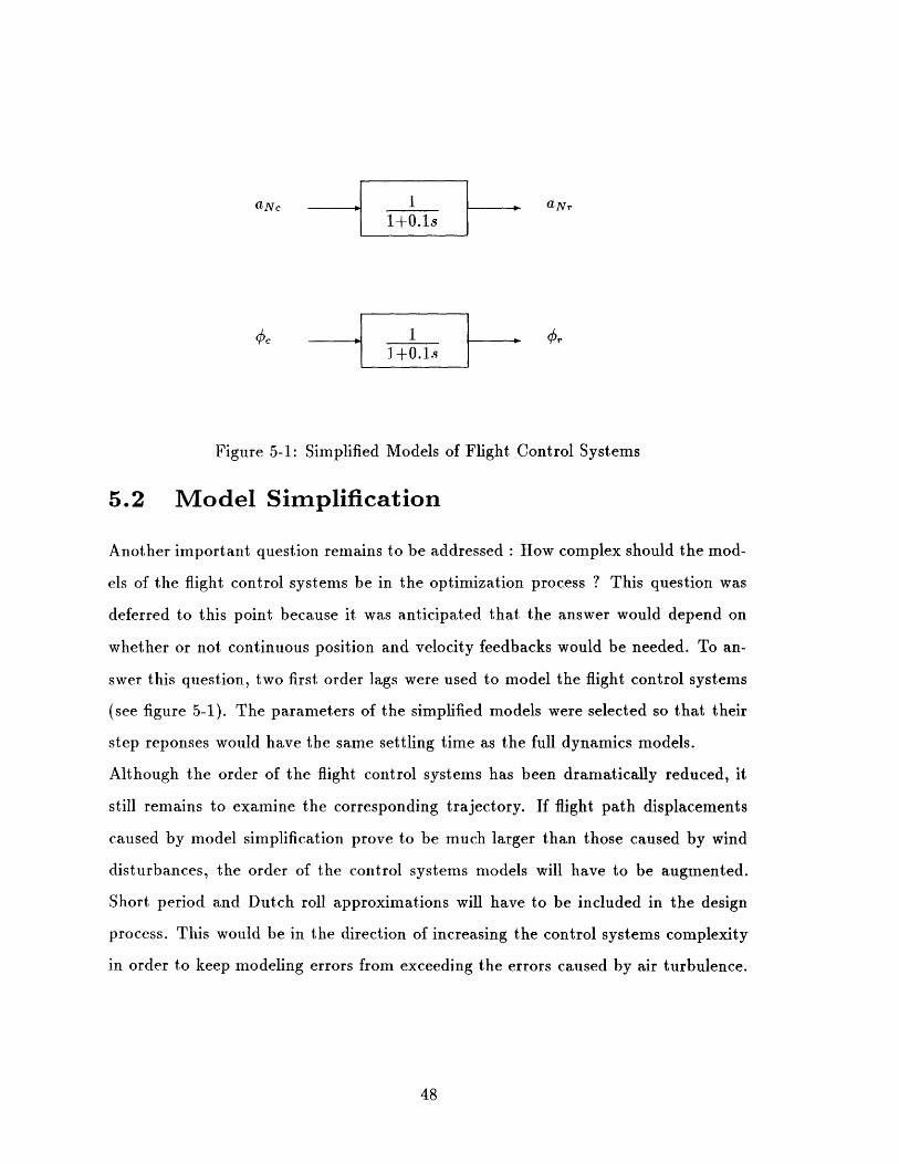
Figure 5-1: Simplified Models of Flight Control Systems

5.2 Model Simplification

Another important question remains to be addressed : How complex should the mod-

els of the flight control systems be in the optimization process ? This question was

deferred to this point because it was anticipated that the answer would depend on

whether or not continuous position and velocity feedbacks would be needed. To an-

swer this question, two first order lags were used to model the flight control systems

(see figure 5-1). The parameters of the simplified models were selected so that their

step reponses would have the same settling time as the full dynamics models.

Although the order of the flight control systems has been dramatically reduced, it

still remains to examine the corresponding trajectory. If flight path displacements

caused by model simplification prove to be much larger than those caused by wind

disturbances, the order of the control systems models will have to be augmented.

Short period and Dutch roll approximations will have to be included in the design

process. This would be in the direction of increasing the control systems complexity

in order to keep modeling errors from exceeding the errors caused by air turbulence.

The validity of the models in figure 5-1 is determined by examining the trajectory

deviations due to modeling errors. It is expected that modeling restrictions will

be alleviated by requiring position and velocity feedbacks. This observation is based

upon the sensitivity decrease of the aircraft's trajectory to modeling errors due to such

feedbacks. Figures 5-6 and 5-7 show the vertical displacement errors generated by air

turbulence and modeling errors respectively. Similar plots describing the horizontal

displacement errors are presented in figures 5-8 and 5-9. Continuous feedbacks of

position and velocity errors are used in each case.

It is obvious that errors resulting from simplified modeling are of the same order

as those due to air turbulence. Therefore, it would be unnecessary to increase the

complexity of the flight control systems for the purpose of achieving a more accurate

trajectory following. As a concluding remark, it should be added that first order lags

are the most simple representation into which models of flight control systems could

be cast.

2 4 6 8 10 12TIME IN (SEQ

Figure 5-2: Vertical Sharp-Edged Gust

TIE IN (SEC

Vertical Response with Positiorn

.....

...............................

. . .. . ........... ; .... . .... ......

14 16 18 20

|

Figure 5-3: Aircraft and Velocity Feedback

I r I , .

... ............ ................ .

......................

;

16 18 20

TIME IN (SEC)

Figure 5-4: Lateral Sharp-Edged Gust

16 18 20

TIME IN (SEC)

Velocity Feedbacks

U

TIME IN (SEC)

Figure 5-6: Vertical Displacement Error Due to Wind Gust

I S 4 6 8 10 12 14 16 18 20

TIME IN (SEC)

Figure 5-7: Vertical Displacement Error Due to Modeling

2 4 6 8 10 12 14 16 18 20

TIME IN (SEC)

Figure 5-8: Horizontal Displacement Error Due to Wind Gust

U 2 4 6 8 10 12 14 16 18 20

TIME IN (SEC)

Figure 5-9: Horizontal Displacement Error Due to Modeling

2 4 6 8 10 12 14 16 18 200

Chapter 6

Conclusions and

Recommendations

6.1 Summary of Results

The minimum degree of complexity of the flight control systems models needed in the

optimization process was determined in the context of position and velocity feedbacks.

Since the aircraft is flying at very low altitudes, it was expected that position and

velocity monitoring are needed to suppress the effects of wind disturbances. Stochastic

and deterministic analyses of air turbulence were carried out and specific wind gust

models were simulated.

Normal acceleration and bank angle command updates were used to minimize the

sensitivity of the aircraft's trajectory against wind-induced deviations. The updates

were based upon position and velocity errors between the actual flight path and the

one predicted by the trajectory planner.

Once the computed trajectory was followed closely, even in the presence of wind gusts,

simplified flight control systems models were developed. Use of the simplified models

in the optimization process was justified by comparing trajectory deviations due to

modeling errors to those that are due to air turbulence.

|

6.2 Further Research

Although it was possible to keep the complexity of the flight control systems models at

a minimum, the issue of timely command generation remains to be investigated. This

timeliness is directly associated with the mission success through avoidance of ground

threats. Unless a powerful computer on board is used in the optimization process, a

"back-up unit" must be available. The task of this unit would be to develop a reason-

able strategy ensuring the safety of the mission until the optimal command history is

available. It is expected that such strategy would account for terrain nature and the

distribution of nearby threats. For instance, if the aircraft is flying over a flat terrain

with widely dispersed ground threats, a sensible strategy might be to implement the

most recent command history as the last waypoint is passed until convergence of the

optimization algorithm is reached.

In this research, as well as in previous works [1, 2], it was assumed that the waypoints

distribution is two dimensional. In reality, the waypoints generated by the goal point

planner are depicted in three dimensions. A similar assumption applies to the threat

database. A substantial work might be concentrated on a reliable command genera-

tion taking into account a three-dimensional threat database. Another direction for

further research might be to simplify the optimization process. Reduced computa-

tional tasks translate into rapid convergence and, consequently, relieving the need for

a "back-up unit".

Finally, it would be interesting to implement the concept of the mission planning

system in real-time. Using simplified models of the flight control systems, the aircraft

response to the generated commands should be evaluated via comparing the actual

flight path to the one predicted by the trajectory planner.

Bibliography

[1] Alexander, J.R., Aircraft Command Interface for a Real-Time Trajectory Plan-

ning System, Master's Thesis, Massachusetts Institute of Technology, 1988.

[2] Walker, W.J., Flight Control Command Generation in a Real-Time Mission

Planning System, Master's Thesis, Massachusetts Institute of Technology, 1990.

[3] Etkin, B., Dynamics of Flight, Wiley, New York, 1959.

[4] Hoblit, F.M., Gust Loads on Aircraft : Concepts and Applications, AIAA Press,

Washington, DC, 1988.

[5] Freudenberg, J.S., and D.P. Looze, Frequency Domain Properties of Scalar and

Multivariable Feedback Systems, Springer-Verlag, 1988.

[6] Boyd, S. and Desoer, C.A., Subharmonic Functions and Performance Bounds on

Linear Time-Invariant Feedback Systems, IMA Jour. of Infor. and Contr., 1985.

[7] McRuer, D., I. Ashkenas, and D. Graham, Aircraft Dynamics and Automatic

Control, Princeton University Press, Princeton, NJ, 1973.

[8] Nelson, R.C., Flight Stability and Automatic Control, McGraw-Hill, New York,

1989.

m