Gradient Theory of Optimal Flight Paths HENRY J. KELLEY1

G r u m m a n Aircraft Engineering Corp. Bethpage, N. Y.

An analytical development of flight performance opt imizat ion according to the method of gradi­ents or "method of steepest descent" is presented. Construction of a min imiz ing sequence of flight paths by a stepwise process of descent along the local gradient direction is described as a computa ­tional scheme. Numerical application of the technique is i l lustrated in a s imple example of orbital transfer via solar sail propulsion. Successive approximations to m i n i m u m t i m e planar flight paths from Earth's orbit to the orbit of Mars are presented for cases corresponding to free and fixed bound­ary conditions on terminal velocity components .

THE PAST decade has seen considerable progress in techniques for the determination of flight paths which are

optimal in the sense of various performance criteria. Treat­ments have employed almost exclusively the classical "in­direct" method of the calculus of variations which is based on the reduction of variational problems to differential equa­tions. A number of works on this subject are listed in (1 through 9).2 An excellent bibliography is presented in the survey paper of (10).

Although many interesting results have been forthcoming from analytical solutions of the Euler-Lagrange differential equations governing optimal flight, the idealizing assump­tions usually invoked limit their applicability in practical situations. Under more realistic assumptions, a numerical attack on these equations is required, and in this approach a serious difficulty may arise in the satisfaction of two-point boundary conditions. [See, for example, (11, 12 and 13).] This difficulty becomes a limiting factor where the order of the differential equations governing the basic system is four or higher.

Attention is directed in the present work to one of the direct methods of the calculus of variations, namely the method of gradients or "method of steepest descent," which offers cir­cumvention of the two-point boundary value difficulty. The method also possesses the attractive feature of simultaneous optimization with respect to configuration parameters.

The notion of descent along the gradient direction was originally introduced by Hadamard in connection with mathematical existence proofs (14). Only in recent years has it found practical application to multivariable minimum problems of ordinary calculus (15) and to solution of systems of algebraic equations (16, 17) and integral equations (18).

The main idea of the present treatment stems from material presented by Prof. R. Courant in a 1941 address to the Ameri­can Mathematical Society (19). An application of the gradient method to fixed end-point variational problems has been given by Stein (20). Our extension of the gradient idea to the case which includes differential equations as subsidiary condi­tions is heuristic in character.

Problem Formulation

For present purposes it will be assumed that the system of differential equations to be satisfied along the flight path is

Presented at the ARS Semi-Annual Meeting, May 9-12, 1960, Los Angeles, Calif.

1 Section Leader, Systems Research. Member ARS. 2 Numbers in parentheses indicate References at end of paper.

given in first-order form

(Xi, . . ., Xn, V, t) 1, [1]

These equations relate velocities and positions, forces and accelerations, mass and flow of propellants and coolants, and the like. xm may be termed problem variables, and y the control variable. Differentiation with respect to the inde­pendent variable, time t, is denoted by a superscribed dot.

An important class of problems is that in which the per­formance quantity to be minimized is expressed as a func­tion of the final values of the variables xm and t

P = P(xlf, . 0) [2]

At a specified initial time to as many as n boundary condi­tions on the xm may be stipulated. Since an entire function y(t) is at our disposal, we may reasonably consider problems in which numerous conditions are imposed upon the xm at various subsequent t values. In the following we will restrict attention to conditions imposed at the terminal point of the flight path. Among the n + 1 quantities consisting of the n final values of the xm plus the final time tf, no more than n relations may be specified in order that the value of P not be predetermined.

Neighboring Solutions—^Variations

We now assume that a solution of Equations [1 ] is available which satisfies the boundary conditions but which does not minimize P. Denoting the solution by xm = xm(t), y = y(t), we examine behavior in the neighborhood of this solution by setting xm = xm + dxm, y = y + 8y and linearizing

. A dgm OXm = 1_J ^ °X3 ~T

dgm

by ty m = 1, [3]

The partials of gm are evaluated along xm = xm, y = y and are therefore known functions of the independent variable t. The functions 8xm and by are the variations of xm and y in the neighborhood of xm, y.

A formal solution of Equations [3] may be written in the form

dXm = ] C fopo£mp(t) + I Mm(7 39 = 1 Jto

t r)8y(r)dr

m = 1, . . ., n [4]

where the first member represents solution of the homogeneous system of equations and the second a superposition of control variable effects. The functions /um are Green's functions or in-

OCTOBER 1960 947

Dow

nloa

ded

by U

NIV

ER

SIT

Y O

F C

AL

IFO

RN

IA -

DA

VIS

on

Janu

ary

31, 2

015

| http

://ar

c.ai

aa.o

rg |

DO

I: 1

0.25

14/8

.528

2

fluence functions; ^m(r, t — r) may be thought of as the solution for 8xm corresponding to 8y a uni t impulse (Dirac delta function) introduced a t t ime r (21).

Since interest centers on final values of xm, we evaluate the expressions [4] a t t = tf; however, to cover the possibility of a variable end point, tf = lf -{- 8t/, a first-order correction term must be included

n fir 8xmf = E top&mvOi) + T Vmir, 1/ — T)8y(r)dT + xmf8tf

v = \ J u

= E fap0£mp(h) + I »m(T, If — T)8y(r)dr + gmf8tf P = i J t o

m = 1, . . ., n [5]

where gmf = gm(xlf, . . ., xnf, yf, tf).

Computation of the Functions \xm

Since computat ion of the functions AiTO(r, t — r) over a complete range of both arguments is unnecessary, only their evaluation a t t = tf required for subsequent calculations, it is reasonable to seek a means for performing the special compu­tat ion which avoids the labor of the more general one. The following development relates the functions /*OT(T, If — r) to solutions of a system of equations adjoint to the system [3] through an application of Green's theorem. The scheme em­ployed is due to Bliss, as reported by Goodman and Lance (22).

We rewrite Equat ions [3] employing a subscript notat ion suitable to our immediate purpose

^ *Qi *Qi 8±i = E ^ dxJ + ^ dV i = l , . . ., n

j = 1dxj by;

and write the system of equations adjoint to this system

Ai = - L — Aj i = 1, . . ., n j = i OXi

which is obtained by transposing the matr ix of coefficients and changing the sign.

The solutions of the two systems are related by

[6]

[7]

d-± \<Sxt = ± *<*-'Sy dtf?! i = 1 by

[8]

After integration of both left and right members between definite limits U and lf) we find

E Hb)tei(l,) - E \i(fo)Sxi(to) = I / E ^i—^^ydt [9] 1=1 *=i J h %=i dy

This is the one-dimensional form of Green's theorem (22). We now consider numerical solutions of the adjoint system

with all boundary values specified a t t = tf. To the special solutions corresponding to

\i(tf) = 0 t V w i \%(if) = 1 i = m

[10]

we assign the symbols \i(m\f). In this fashion n expressions for the values of the 8xm{lf) are obtained from [9]

te~(h) = E X/m)(*o)fc(*o) + P E *i(m)^rtydt

m = 1, . . ., n [11]

By comparison with Equat ions [5] it may be seen t h a t the de­sired relation between the /xTO(r, lf — r) and the X/m) is the following one

Mm (r, If — T) = E ^ dy

and, also, t ha t the £mp(i/) of Equat ions [5] is equal to \pim)(to).

In the preceding development the choice of symbols A for the variables of the adjoint system is deliberate, for Equat ions [7] are precisely those governing the Lagrange multiplier functions of the "indirect" theory. We note the important distinction, however, t ha t the coefficients of [7] employed in the "indirect" theory are evaluated along a minimal solution of Equat ions [1], whereas in gradient computat ions they correspond to nonminimal pa ths .

Descent Parameter

Following Courant (19), we now introduce a parameter a as a second independent variable, and seek a functional de­pendence of the control variable y(t, a) on this parameter such t h a t the derivative of the performance quan t i ty dP/da is negative. I n fact, within the restrictions imposed by the boundary conditions and the system equations, we shall a t t empt to make the slope of descent dP/da "as steep as possible."

To enable operation within the restrictions just mentioned, we break down the control variable y as follows

y(f, a) = 4>{t, a) + E aMfS) [13] ff = i

Here the fg(t) are a set of known linearly independent func­tions of t. Our intention is t h a t the coefficients aq of the second member of [13] be sacrificed to the fulfillment of boundary conditions, the number r being chosen appro­priately for this purpose. This will leave the function </> free for the minimization of P.

We now take the derivatives of various quanti t ies with re­spect to a and evaluate them a t a = a, corresponding to the nonminimal solution xm(t, a) = xm, y(t, a) = y introduced in the preceding section. For a — a = Aa small, the varia­tions appearing in Equat ions [5] m a y be identified as

Xm0 + 8xmo = xmo + (dxmJda)Aa m = 1, . . ., n [14]

+ 8xmf = xmf + (dxmf/da)Aa m = 1, . . ., n [15]

tf = If + 8tf = If + (dt//d*)A<r [16]

y = y + $y=zy+ (dy/da-)Aa

= $ + E agm + q = l Oa q=z da

Aa [17]

Equations [5] then take the form

dxmf \^ dxPo C

Oa v = \ da Jto

7 / 7 \ ^ Vm{T, tf ~ T) — G

Oa

lr +

t P fttf^(r,lf~r)f,(r)dr + g,nf

l = l aa J to

dtf

da

., n [18]

Boundary Conditions

We consider boundary conditions of the separated type, i.e., equations relating either initial values or final values. Boundary values may be variable on a surface, typified by

<J\Xuj) Xvf) If) vJ [19]

in which case the following linear combination of derivatives mus t vanish

m = 1, . . ., n [12] d3 _ d3 dxUf , d3 dxvs c)3 dtf _

da OXu da dxv da dtf da [20]

948 ARS JOURNAL

Dow

nloa

ded

by U

NIV

ER

SIT

Y O

F C

AL

IFO

RN

IA -

DA

VIS

on

Janu

ary

31, 2

015

| http

://ar

c.ai

aa.o

rg |

DO

I: 1

0.25

14/8

.528

2

In this expression the partial derivatives of 3 are evaluated at could be expressed as %uf == %"Ufj *£"i>f == % vf ano. t/ == tf>

In the case of fixed boundary conditions of the form xUf = xUf = constant, tf = tf = constant, the relations to be satisfied

dP da

= grad P- — da

[28]

take the simple form

§* = 0 or f' = 0 da da

[21]

As many as n final conditions, fixed or of the form [19] may be specified, as mentioned earlier. Where fewer than this number are specified, we speak of "free" or "open" boundary values.

At the initial point similar freedom of choice may exist among the n initial values of the xm, the only difference here being that to will usually be fixed.

Gradient of P

Upon inspection it may be noted that there are n equations of the form [18] and at most 2n equations for boundary values, making a possible total of 3n equations. These relate 2n + 1 derivatives of the xmo, xmf and tf, the r derivatives of the aq and integrals containing d(f>/ba. We accordingly choose the number r of the aq as r = n — 1 — s, where s is the number of open boundary conditions. Thus the system of equations will be determinate for arbitrary b^/ba.

These equations may be arranged as a linear simultaneous system

AZ = B [22]

where Z has Sn — s elements consisting of the derivatives with respect to a of xmo, xmf, tf and aq. The matrix A is square and contains among its elements the quantities £mp, gmf, the 3 partials, and integrals of products jnmfq, all of which are known. The column B includes integrals containing b4>/ba in their integrands. The solution

Z = A~lB [23]

may be obtained through matrix inversion or equivalent proc­esses. The matrix A expresses the relationship between small shifts in boundary values and small adjustments in the con­trol function (through the aq) to deal with them. Hence in normal circumstances A will be nonsingular.

The derivative with respect to a of the quantity P to be minimized

*P _ &L ^n 4. dP dXnf d P ^ da dxif da ' ' ' bxnf da bt/ da

[24]

may now be expressed in terms of known quantities and inte­grals containing b<f)/ba according to the solution [23]. It will take the form of a linear combination of the integrals

dP da

Vm{T, tf — T) — l Oa tc.s:

1 = 1 J h

ressed as a (T J to [_ms=1

which may be expressed as a single integral

r) dP

d7

[25]

[26]

By analogy with a characteristic property of a vector gradi­ent, we are now prepared to identify the gradient of P with respect to the function 4>. [See p. 222 of the Courant-Hilbert English edition, (23), also (19).] If 0 were a vector possessing a finite number of components </>;, i = 1, . . ., j , the derivative of P with respect to a

dP da i = i d(j)i da

[27]

If 4>{t, a) is a continuous function, and P a functional of 0, as in the case of present interest

da Oa [29]

and the function occurring in product with d<f>/da, which we denote [P]</>, may be regarded as the gradient of P by ex­tended definition.

Thus for the problem at hand it is evident from Equation [26] that

IP]* = Z Cm/xm(r, 1/ - r) m = l

[30]

is the gradient of P. Were the solution xm = xm, y = y such as to minimize P,

contrary to our assumption, the gradient [P]<t> would vanish. If our development were to parallel the classical or "indirect" approach, the construction of a solution would be sought from the vanishing of [P]^ for which P is stationary and possibly a minimum. Thus [P]0 is in some sense an Euler expression and the equation [P]^ = 0 and the relations [23] have an equiva­lence to the Euler-Lagrange equations and transversality conditions of the "indirect" theory.

Descent Process

Returning momentarily to the elementary geometric con­cept of a vector gradient, we regard P(<f>i, . . ., <f>j) as a surface, and starting from P(0i, . . ., 0y) we move a point along this surface so that P and fa become functions of a time parameter a. Then the velocity of ascent or descent along a line on the surface is as given by Equations [27 and 28]. We now choose the line along which the descent is as steep as possible, characterized by

^ = fc d p

[31]

where k positive corresponds to ascent and k negative to descent.

It is clear that in this continuous process, wherein the point moves according to the system of ordinary differential equa­tions [31], the process will for cr—^ °o approach a position for which grad P = 0, if P is bounded below.

This elementary idea may be generalized to the present variational problem according to the extended interpretation of the gradient of P, Equation [29]. We set

^ =k[PU= -[P]+ Oa

[32]

and starting from the nonminimal solution a = a, <t> = 0, xm — evaluate these quantities on a continuous basis

as the parameter a increases. Thus the continuous version of descent along the gradient

requires numerical treatment of a partial differential equation for <j>(t, a) with determination of <f>(t, °°) the ultimate objec­tive.

Stepwise Version

As an alternative to the continuous procedure given by Equation [32], we may elect to proceed stepwise, correcting a set of approximations to the solution [P]^ = 0 by corrections proportional to the negative of the gradient

4> (i+D 0 (0 _ [PU*<T [33]

OCTOBER 1960 949

Dow

nloa

ded

by U

NIV

ER

SIT

Y O

F C

AL

IFO

RN

IA -

DA

VIS

on

Janu

ary

31, 2

015

| http

://ar

c.ai

aa.o

rg |

DO

I: 1

0.25

14/8

.528

2

MARS ORBIT

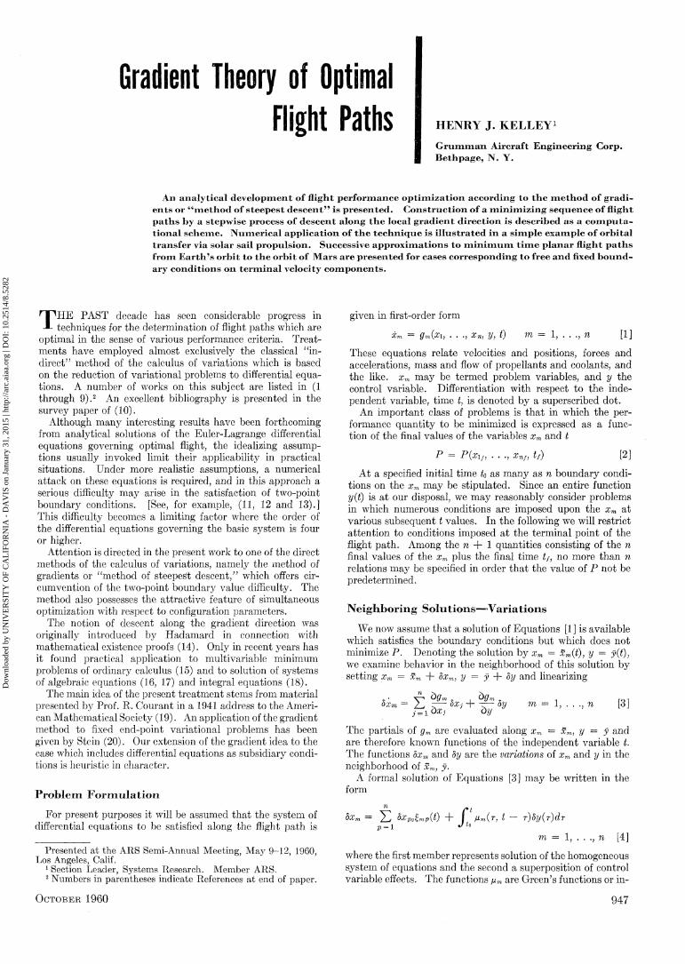
Fig. 1 Orbital transfer schematic

After choice of step size Aa and evaluation of 0 ^ + 1 ) and the a<z( t+1\ the functions xm^+1^ would be obtained from numeri­cal integration of the basic system Equations [1 ] and P ^ + ^ de­termined from the values at £/*+1) .

Since the determination of the gradient [P]<j> is expensive in terms of volume of numerical computations, it would seem desirable to exploit each calculation of local gradient direction of the utmost, taking A a- as large as possible. A procedure em­ployed in some applications (17) is to follow the local gradient direction until the function P reaches a minimum. Such a procedure could be implemented by numerical integration of Equations [1] for a number of values of Aa and selection of the value of Aa for minimum P.

A possible pitfall of such a scheme of operation is that the boundary conditions, having been satisfied only in linearized version (Eq. [20]), may long since have been violated before minimum P is reached (24). Thus the choice of Aa involves a compromise which must be decided in the particular appli-tion at hand. If the minimum P rule is employed for choice of Aa, the boundary conditions must be restored by a correc­tion cycle designed to recover from the departures.

After such restoration has been accomplished, for example via the coefficients aq, the solution so obtained takes on the role of xm, y for the computation of a new local gradient direc­tion.

Convergence

The convergence of the descent process has been investi­gated by Stein for a case not complicated by subsidiary condi­tions (20); his conclusion was that the process will converge if the functional whose minimum is sought is bounded below. In the process described in the preceding sections, the ques­tion of convergence is intimately related to the success of the technique for maintaining or correcting the boundary values at the terminal point.

The possibility of correcting small departures in terminal values of the xm through small changes in the coefficients ag

can be shown to hinge on the nonvanishing of the determinant of the matrix A of Equation [22]. In certain cases a tendency of this determinant to become small may be observed as a minimum of P is approached. Where the difficulty is acute, the behavior may be likened to breakdown of a first-order differential correction scheme for guidance along the trajec­tory.

This type of behavior is a close relative of the conjugate

end-point phenomenon of classical variational theory. If an extremal through point 1 has on it a contact point 2 with the envelope of a family of extremals through 1, then point 2 is said to be conjugate to point 1. The term conjugate end points refers to specification of boundary values at two such points as 1 and 2. The reader is advised to consult the text of Bliss (25) for the analytical basis of conjugate point theory.

The relevant test of the classical theory, the necessary con­dition of Jacobi, employs a determinant as a criterion. The requisite analysis amounts to investigation of optimal dif­ferential corrections of terminal values. Thus a matrix which is the optimal correction analog of the matrix A is set up, and the criterion of the Jacobi test is the nonvanishing of the de­terminant of this matrix at points along the extremal up to the terminal point of interest. Vanishing at the terminal point indicates that the end points are conjugates, and the necessary condition is fulfilled in borderline fashion. Computational procedures for applying the Jacobi test are of some interest; however, the acquisition of a "test specimen" solution requires that any convergence difficulty encountered in the descent process first be overcome.

Thus a possibility of convergence difficulty arises in conju­gate end-point cases if the functions fq selected happen to re­semble the optimal correction functions of the indirect theory. There are certainly other possibilities for unfortunate choice of correction functions. Computational experience will be required to establish guidelines on this matter.

Configuration Parameters

In many practical engineering applications, optimal per­formance is sought not only in terms of flight path selection but also in terms of parameters influencing vehicle configura­tion. We have, for clarity, avoided complicating the preced­ing analytical work by such considerations. It is an easy matter, however, to add terms to Equations [5] of the form (dxmf/dei)8ei and to carry them through along with con­straints relating ei} thus forming a basis for simultaneous optimization of configuration and flight path. The slopes dxmf/dei are probably best determined by numerical integra­tion of Equations [1 ] for small changes in e*.

Solar Sai l ing Example

For the purpose of exploring the computational aspect of the gradient optimization technique, we have chosen a planar case of transfer between planetary orbits by means of the in­teresting solar sailing scheme. The potential capabilities of solar sail propulsion have been investigated in the papers of Garwin (26), Cotter (27), Tsu (28) and London (29). This problem has the simplicity appropriate to an exploration of method, yet sufficient complexity to render analytical solu­tion quite difficult unless drastic simplifications are intro­duced.

The equations of motion and kinematic relations are given in a notation nearly the same as that of Tsu (28). With reference to the schematic of Fig. 1, these are as follows:

Radial acceleration

U = & = R~ AO\R) + a VR) 'C0S °\ [ 3 4 ]

Circumferential acceleration

uv i) = g2 = - — - a(Ro/R)2 sin B cos2 6 [35]

K

Radial velocity

R = g3 = u [36]

Circumferential angular velocity

t = v/R [37]

950 ARS JOURNAL

Dow

nloa

ded

by U

NIV

ER

SIT

Y O

F C

AL

IFO

RN

IA -

DA

VIS

on

Janu

ary

31, 2

015

| http

://ar

c.ai

aa.o

rg |

DO

I: 1

0.25

14/8

.528

2

Since the heliocentric angle \p does not appear in the first three equations, and will not appear in the s ta tements of boundary conditions to be considered, Equat ion [37] may be ignored for purposes of gradient optimization. This amounts to the assumption tha t terminal matching of the heliocentric angles of vehicle and " t a rge t " planet is accomplished by selec­tion of launch t ime.

Seeking minimum-time transfer, we identify the functional P a s

P = tf [38]

The functions u, v, R are the variables xm of the theoretical development, and the sail angle 6 appears in the role of the control variable y.

As initial conditions we specify velocity components u, v and radius R corresponding to motion in Ea r th ' s orbit ap­proximated as a circle

£o = 0 [39]

u(0) = UQ = uE = 0

V(0) = VQ = VE

R(0) = Ro = RE

[40]

[41]

[42]

We consider terminal conditions corresponding to arrival a t the orbit of the planet Mars (also taken as a circle) with pre­scribed velocity components

U(tf) = Uf

V(tf) = Vf

R{tf) = Rf = RM

[43]

[44]

[45]

For fixed boundary values of u, v and R, the equations cor­responding to Equat ions [5] of the preceding theoretical de­velopment are

8iif = 1 jjudddr + (jifUf = 0

bVf = Jo ^Qdr + g2f8tf = 0

oRf = f'f tizbddr + gSfdtf = 0

[46]

[47]

[48]

In this case the number of functions fg and coefficients aq

required is

3 - 1 - 0 [49] r = n — 1 — s

We select the functions fg as

Mt) = l [50]

MO = t* [51]

and the control function 6(f) is broken down as

e = <j> + ait + a2t2 [52]

The system of equations corresponding to Equat ion [22] simplifies to

a 'ff \ dai ( (h \ <kh , . dtf

L

a,7wo:f+a 2 ^ ^ d a 2 i -

•lld2dr ) — + g2f

vi —dr [53] u Oa

(fof T^TY£ + (fof T2^dT)d£ + dtf_

rda

- ; . Ms ^ dr [55]

0 Oa

This 3 X 3 case may conveniently be inverted analytically. There seems little point in listing the inverse e lements here, however.

fdai

| da

1 da2

1 da

\ d t f

\_da _

= -

"

C

/mi ^— dr Jo ^da rtr dcf>

Jo ^Zad'>

rif d 0 . J 0 MB-dr da

[56]

The slope of descent dtf /da is given by

dh _ __ rif

da ~ JO

and the gradient of P by

[P]<t> — ""(ftlMl + C32/i2 + C33M3)

Accordingly we set

d<t>/da = - [ P ] 0 = CSIMI + C32M2 + C*m

{Czini + C32M2 + CW3) T~ O r [57]

[58]

[59]

and proceed with stepwise descent as in Equat ion [33]. A particularly suitable case for a first illustration of com­

putat ional technique is the one in which terminal velocity components are unspecified—"free" boundary conditions. Here Equat ions [46 and 47] may be deleted and

r = n - l ~ s = 3 - l - 2 = 0

so t h a t no functions fq are needed. Hence

[60]

and

d0

da

dtf

da

_ M3_

03/

M3' dr

[61]

[62]

in this case. Computat ions have employed numerical values of the

various constants from Tsu 's paper, with

a = 0.1 cm/sec 2 = 3.28 X 10~3 fps2

This value corresponds to about 10 ~4 g thrus t acceleration developed by the sail when oriented broadside to the sun (0 = 0) a t Ea r th ' s orbit radius, or about 17 per cent of the sun's gravitat ional a t t ract ion.

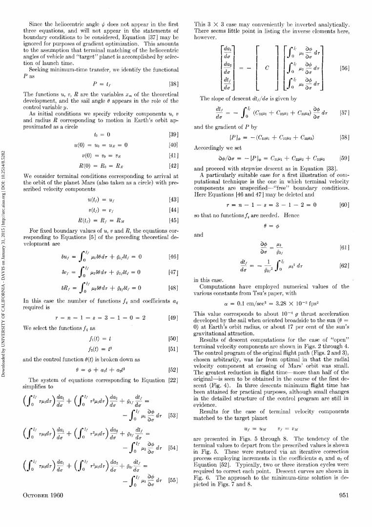
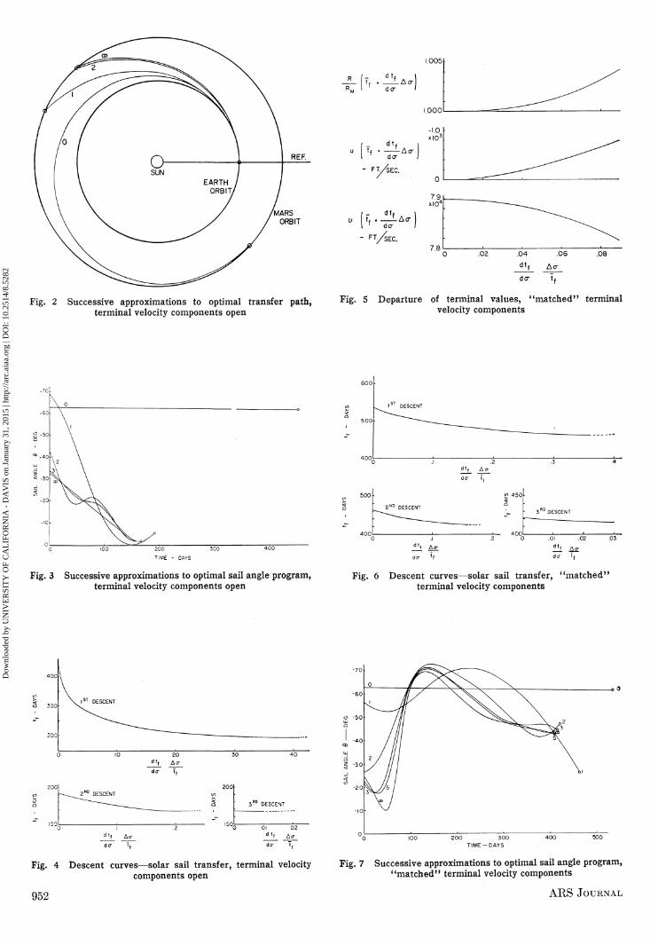
Results of descent computat ions for the case of "open" terminal velocity components are shown in Figs. 2 through 4. The control program of the original flight pa th (Figs. 2 and 3), chosen arbitrarily, was far from optimal in t h a t the radial velocity component a t crossing of Mars ' orbit was small. The greatest reduction in flight t ime—more than half of the original—is seen to be obtained in the course of the first de­scent (Fig. 4) . In three descents minimum flight t ime has been at ta ined for practical purposes, al though small changes in the detailed structure of the control program are still in evidence.

Results for the case of terminal velocity components matched to the target planet

Uf = UM Vf = VM

are presented in Figs. 5 through 8. The tendency of the terminal values to depart from the prescribed values is shown in Fig. 5. These were restored via an i terative correction process employing increments in the coefficients ai and a2 of Equat ion [52]. Typically, two or three iteration cycles were required to correct each point. Descent curves are shown in Fig. 6. The approach to the minimum-time solution is de­picted in Figs. 7 and 8.

O C T O B E R 1960 951

Dow

nloa

ded

by U

NIV

ER

SIT

Y O

F C

AL

IFO

RN

IA -

DA

VIS

on

Janu

ary

31, 2

015

| http

://ar

c.ai

aa.o

rg |

DO

I: 1

0.25

14/8

.528

2

MARS

ORBIT

Fig. 2 Successive approximations to optimal transfer path, terminal velocity components open

-Ao -

IOOO

T dcr J

FT/SEC.

„ K . ^ - A c r ;

" FT/SEC.

Fig. 5 Departure of terminal values, "matched" terminal velocity components

200 300

TIME - DAYS

Fig. 3 Successive approximations to optimal sail angle program, terminal velocity components open

2 N 0 DESCENT

d 1 f A C T

Fig. 6 Descent curves—solar sail transfer, "matched" terminal velocity components

IS T DESCENT

0 2 f f Ac-

Fig. 4 Descent curves—solar sail transfer, terminal velocity components open

e>

Q I

I

AN

GLE

S

AIL

-70

-60

-50

-40

-30

-2 0

-10

0

,

2 /

^ V

//•5 /

^—^\

100 2 0 0 3 0 0

T I M E - D A Y S

Fig. 7 Successive approximations to optimal sail angle program, "matched" terminal velocity components

952 ARS JOURNAL

Dow

nloa

ded

by U

NIV

ER

SIT

Y O

F C

AL

IFO

RN

IA -

DA

VIS

on

Janu

ary

31, 2

015

| http

://ar

c.ai

aa.o

rg |

DO

I: 1

0.25

14/8

.528

2

MARS ORBIT

Fig. 8 Successive approximations to optimal transfer path, "matched" terminal velocity components

The first a t t emp t a t computations for this "matched ve­loci ty" case employed functions fq constant and linear with time. This met with near zero determinant difficulty of the type discussed earlier. The combination of linear and square-law corrections indicated in the foregoing was successfully used to avoid this difficulty.

C o n c l u d i n g R e m a r k s

Attent ion has been confined in the preceding development to the main ideas of the gradient technique. The extension to cases involving several control variables offers no particular difficulty. The limited computat ional experience reported here suggests t ha t the gradient technique may be a useful one in applications, and particularly in those presenting difficulty when the classical " indirect" approach—numerical integration of the Euler-Lagrange equations—is used. Apar t from the feature of surmounting the two-point boundary value dif­ficulties of such cases, the gradient method may be particu­larly appropriate in distinguishing between minimal solutions of the Euler-Lagrange equations and those which are merely stationary.

A c k n o w l e d g m e n t s

The writer is pleased to acknowledge the contributions of Messrs. William P . O'Dwyer and H . Gardner Moyer of Grum-man 's Computat ion Facility in handling the computat ional phase of this s tudy on the I B M 704, and of Mrs . Agnes Zevens of the Systems Research Section in checking and preparing the numerical results for publication.

N o m e n c l a t u r e

y Qm

t P 8xm

Mm

&y

problem variables control variable functions of xm and y appearing in basic system

equations time function of final values of xm to be minimized variations of xm and y functions appearing in the solution of Equations

[3] Green's functions in the solution of Equations [3] variable of integration

Ao 3 A Z

k et u V

R

A,

u, v\

Subscripts

f 0 m, p. q, r)

E M (•) (-) ( i ) (m)

variables of the adjoint system, Equation [7] descent parameter auxiliary control variable, Equation [13] known linearly independent functions of t coefficients of the functions fq

increment in a-function relating boundary values of xm and t matrix of coefficients, Equation [22 ] column matrix having dxmJdv, dxmf/da, dtf/da

and dag/da as elements, Equation [22] column matrix containing integrals of fxm(dcf>/d<T)

products, Equation [22] coefficients of the linear combination of /*m, Equa­

tion [26] gradient of P , Equation [30 ] proportionality constant of descent configuration parameters radial velocity component (see Fig. 1) circumferential velocity component (see Fig. 1) radial distance to sun (see Fig. 1) heliocentric angle acceleration due to sun's gravitational attraction

at Earth 's radial distance thrust acceleration of radially oriented solar sail

at Earth 's radial distance sail angle measured from radial orientation

denotes final value denotes initial value

general indexes

Ear th Mar denotes time derivative denotes nonminimal solution denotes value at ith step denotes special functional notation, explained by

Equation [10]

R e f e r e n c e s

1 Hestenes, M. R., "A General Problem in the Calculus of Variations with Applications to Paths of Least Time," Rand RM-100, March 1950.

2 Garfinkel, B., "Minimal Problems in Airplane Performance," Quart. Appl. Math., vol. 9, no. 2, 1951.

3 Cicala, P., "Le Evoluzioni Ottime di un Aereo," Atti della Accademia delle Scienze di Torino, Classe di Scienze Matematiche, Fisiche e Naturali, vol. 89, 1954-1955. (Translated as NASA Technical Translation TTF-4, Oct. 1959.)

4 Miele, A., "An Extension of the Theory of the Optimum Burning Program for the Level Flight of a Rocket-Powered Aircraft," Purdue Uni­versity School of Aeronautical Engineering, Rep. no. A-56-1, Technical Note no. AFOSR-TN-56-302, June 1956; also J. Aeron. Sci., vol. 24, no. 12, Dec. 1957.

5 Breakwell, J. V., "The Optimization of Trajectories," North American Aviation, Inc., Rep. AL-2706, Aug. 1957; also J. Soc. Ind. Appl. Math., vol. 7, no. 2, June 1959.

6 Okhotsimskii, D. E. and Eneev, T. M., "Some Variation Problems Connected with the Launching of Artificial Satellites of the Earth," Uspekhi Fizicheskikh Nauk, Sept. 1957. (Translated in J. Brit. Interplanet. Soc, vol. 16, no. 5, Jan.-Feb. 1958.)

7 Miele, A., "General Variational Theory of the Flight Paths of Rocket-Powered Aircraft, Missiles and Satellite Carriers," Purdue University School of Aeronautical Engineering, Rep. no. A-58-2, Technical Note no. AFOSR-TN-58-246, Jan. 1958; also Astronautica Acta, vol. IV, fasc. IV, Dec. 1958.

8 Kelley, H. J., "An Investigation by Variational Methods of Flight Paths for Optimum Performance," Sc.D. thesis, Guggenheim School of Aero­nautics, New York University, May 1958. (Published in part as "An In­vestigation of Optimal Zoom Climb Techniques," J. Aero/Space Sci., vol. 26, no. 12, Dec. 1959.)

9 Leitmann, G., "On a Class of Variational Problems in Rocket Flight," Lockheed Missile and Space Systems Division Rep. 5067, September 1958; also J. Aero/Space Set., vol. 26, no. 3, Sept. 1959.

10 Leitmann, G., "The Optimization of Rocket Trajectories—A Sur­vey," in "Progress in the Astronautical Sciences," S. F. Singer, Ed., to appear in 1961.

11 Mengel, A. S., "Optimum Trajectories," Proceedings of Project Cy­clone Symposium 1 on REAC Techniques, Reeves Instrument Corp. and USN Special Devices Center, N.Y., March 15-16, 1951.

12 Irving, J. H. and Blum, E. K., "Comparative Performance of Ballistic and Low-Thrust Vehicles for Flight to Mars," in "Vistas in Astronautics," vol. II, Pergamon Press, N. Y., 1959, pp. 191-218.

13 Faulder^, C. R., "Low-Thrust Steering Program for Minimum Time Transfer Between Planetary Orbits," SAE National Aeronautic Meeting, Los Angeles, Calif., Sept. 29-Oct. 4, 1958.

14 Hadamard, J., "M£moire sur le Problem d'Analyse Relatif a l'Equi-libre des Plaques Elastiques Encastr^es," M6moires presented par divers savants ^strangers a l'Acad£mie des Sciences de l 'lnstitut de France (2), vol.

O C T O B E R 1960 953

Dow

nloa

ded

by U

NIV

ER

SIT

Y O

F C

AL

IFO

RN

IA -

DA

VIS

on

Janu

ary

31, 2

015

| http

://ar

c.ai

aa.o

rg |

DO

I: 1

0.25

14/8

.528

2

33, no. 4, 1908. 15 Curry, H. B., "The Method of Steepest Descent for Non-Linear

Minimization Problems," Quart. Appl. Math., vol. II , no. 3, Oct. 1944. 16 Hestenes, M. R. and Stiefel, E., "Method of Conjugate Gradients

for Solving Linear Systems," Nat. Bur. Standards, J. Research, vol. 49, 1952, pp. 409-436.

17 Forsythe, A. I. and Forsythe, G. E., "Punched-Card Experiments with Accelerated Gradient Methods for Linear Equations," Nat. Bur. Standards, Applied Mathematics Series 39, Sept. 1954, pp. 55-69.

18 Muller, C , "A New Method for Solving Fredholm Integral Equa­tions," New York University Institute of Mathematical Sciences, Division of Electromagnetic Research Rep. no. BR-15, 1955.

19 Courant, R., "Variational Methods for the Solution of Problems of Equilibrium and Vibrations," Bull. A-mer. Math. Soc, vol. 49, no. 1, Jan. 1943.

20 Stein, M. L., "On Methods for Obtaining Solutions of Fixed End-Point Problems in the Calculus of Variations," Nat. Bur. Standards, J. Research, vol. 50, no. 5, May 1953.

21 Friedman, B., "Principles and Techniques of Applied Mathematics," John Wiley and Sons, Inc., N. Y., 1956.

22 Goodman, T. R. and Lance, G. N., "The Numerical Integration of Two-Point Boundary Value Problems," Mathematical Tables and Other Aids to Computation, vol. 10, no. 54, April 1956.

23 Courant, R. and Hilbert, D., "Methoden der Mathematischen Physik," Julius Springer, Berlin, vol. 1, 1924, 1931. (Translated and re­vised edition of vol. 1, Interscience Publishers, N. Y., 1953.)

24 Tompkins, C. B., "Methods of Steep Descent," in "Modern Mathe­matics for the Engineer," E. F. Beckenbach, Ed., McGraw-Hill Book Co., Inc., N. Y., 1956, chap. 18.

25 Bliss, G. A., "Lectures on the Calculus of Variations," University of Chicago Press, Chicago, 1946.

26 Garwin, R. L., "Solar Sailing—A Practical Method of Propulsion Within the Solar System," J E T PROPULSION, vol. 28, no. 3, March 1958.

27 Cotter, T. P., "Solar Sailing," Sandia Research Colloquium, April 1959.

28 Tsu, T. C , "Interplanetary Travel by Solar Sail," ARS JOURNAL, vol. 29, no. 6, June 1959.

29 London, H. S., "Some Exact Solutions of the Equations of Motion of a Solar Sail With Constant Sail Setting," ARS JOURNAL, vol. 30, no. 2, Feb. 1960.

Optimum Thrust Programming of Electrically Powered Rocket Vehicles

in a Gravitational Field C. R. FAULDERS1

North American Aviation, Inc. Downey, Calif.

The general problem of o p t i m u m thrust programming of an electrically powered rocket under the condition of constant je t power is considered. The thrust vector is assumed to be parallel to the instantaneous velocity vector at all t imes . The various opt imizat ion problems possible under these restrictions are shown to be equivalent to maximizat ion of the change in velocity for specified pro­pellant mass and arbitrary range, maximizat ion of range for specified propellant mass and arbi­trary change in velocity, and maximizat ion of the change in velocity for specified range and specified propellant mass . The calculus of variations is employed to obtain analytical expressions for the thrust acceleration program for the foregoing problems wi th a constant gradient of the tangential component of gravitational force. Limit ing values of this gradient for which the tangent ia l c o m ­ponent of gravity can be assumed constant in the derivation of o p t i m u m thrust programs are deter­mined.

ELECTRICALLY powered rocket engines, such as the ion rocket and the plasma rocket, are characterized by a

power source that is separate from the propellant. For a fixed power setting, therefore, the rate of propellant expendi­ture and the exhaust velocity can be varied over wide ranges, and a variety of thrust programs can be achieved. Electrical rockets are presently limited to very low thrust levels of the order of 10 ~3 or 10 ~4 Earth gr's per unit mass of the complete space vehicle. For this reason, an entire mission would generally be carried out under power, with operating times measured in days or weeks.

The various possible requirements for optimum thrust programs are summarized in Table 1, assuming that the total

Received Dec. 8,1959. 1 Research Specialist, Aero-Space Laboratories, Missile Divi­

sion.

time of powered flight is a specified parameter, and that the thrust is always in the tangential direction. The change in vehicle velocity is indicated by AV, the change in position, or range, by As, and the propellant mass by mv.

Table 1

Case 1 2 3 4 5 6 7

Optimum thrust program requirements (total time specified)

AV maximum specified arbitrary arbitrary maximum specified specified

As arbitrary arbitrary maximum specified specified maximum specified

mv

specified minimum specified minimum specified specified minimum

954 ARS JOURNAL

Dow

nloa

ded

by U

NIV

ER

SIT

Y O

F C

AL

IFO

RN

IA -

DA

VIS

on

Janu

ary

31, 2

015

| http

://ar

c.ai

aa.o

rg |

DO

I: 1

0.25

14/8

.528

2