FEYNMAN INTEGRALS AND MOTIVESmatilde/ECMpaper.pdf · FEYNMAN INTEGRALS AND MOTIVES MATILDE MARCOLLI and Beyond the Inﬁnite (Stanley Kubrick, 2001 - A Space Odyssey) Contents 1

FEYNMAN INTEGRALS AND MOTIVES

MATILDE MARCOLLI

and Beyond the Infinite

(Stanley Kubrick, 2001 - A Space Odyssey)

Contents

1. Introduction: quantum fields and motives, an unlikely match 11.1. Feynman diagrams: graphs and integrals 31.2. Perturbative Quantum Field Theory in a nutshell 31.3. The Feynman rules 61.4. Parametric representation of Feynman integrals 71.5. Algebraic varieties and motives 91.6. The mixed Tate mystery: supporting evidence 112. A bottom-up approach to Feynman integrals and motives 122.1. Feynman rules in algebraic geometry 142.2. Determinant hypersurfaces and manifolds of frames 172.3. Handling divergences 193. The Connes–Kreimer theory 203.1. The BPHZ renormalization procedure 203.2. Renormalization, Hopf algebras, Birkhoff factorization 214. A top-down approach via Galois theory 224.1. Counterterms as iterated integrals 244.2. From iterated integrals to differential systems 244.3. Flat equisingular connections 254.4. Flat equisingular vector bundles 254.5. The Riemann–Hilbert correspondence 265. The geometry of Dim Reg 275.1. The noncommutative geometry of DimReg 275.2. The motivic geometry of DimReg 28Acknowledgement 29References 30

1. Introduction: quantum fields and motives, an unlikely match

This paper, based on the plenary lecture delivered by the author at the 5th European Con-gress of Mathematics in Amsterdam, aims at giving an overview of the current approachesto understanding the role of motives and periods of motives in perturbative quantum field

1

2 MATILDE MARCOLLI

theory. It is a priori surprising that there should be any relation at all between such dis-tant fields. In fact, motives are a very abstract and sophisticated branch of algebraic andarithmetic geometry, introduced by Grothendieck as a universal cohomology theory for al-gebraic varieties. On the other hand, perturbative quantum field theory is a procedure forcomputing, by successive approximations in powers of the relevant coupling constants, valuesof physical observables in a quantum field theory. Perturbative quantum field theory is notentirely mathematically rigorous, though as we will see later in this paper, a lot of interestingmathematical structures arise when one tries to understand conceptually the procedure ofextraction of finite values from divergent Feynman integrals known as renormalization.

The theory of motives itself has its mysteries, which make it a very active area of research incontemporary mathematics. The categorical structure of motives is still a problem very muchunder investigation. While one has a good abelian category of pure motives (with numeri-cal equivalence), that is, of motives arising from smooth projective varieties, the “standardconjectures” of Grothendieck are still unsolved. Moreover, when it comes to the much morecomplicated setting of mixed motives, which no longer correspond to smooth projective va-rieties, one knows that they form a triangulated category, but in general one cannot improvethat to the level of an abelian category with the same nice properties one has in the case ofpure motives. See [13], [40] for an overview of the theory of mixed motives.

The unlikely interplay between motives and quantum field theory has recently become anarea of growing interest at the interface of algebraic geometry, number theory, and theoreticalphysics. The first substantial indications of a relation between these two subjects came fromextensive computations of Feynman diagrams carried out by Broadhurst and Kreimer [20],which showed the presence of multiple zeta values as results of Feynman integral calculations.From the number theoretic viewpoint, multiple zeta values are a prototype case of thosevery interesting classes of numbers which, altough not themselves algebraic, can be realizedby integrating algebraic differential forms on algebraic cycles in arithmetic varieties. Suchnumbers are called periods, cf. [38], and there are precise conjectures on the kind of operations(changes of variables, Stokes formula) one can perform at the level of the algebraic data thatwill correspond to relations in the algebra of periods. As one can consider periods of algebraicvarieties, one can also consider periods of motives. In fact, the nature of the numbers oneobtains is very much related to the motivic complexity of the part of the cohomology of thevariety that is involved in the evaluation of the period.

There is a special class of motives that are better understood and better behaved withrespect to their categorical properties: the mixed Tate motives. They are also the kind ofmotives that are expected (see [34], [48]) to be supporting the type of periods like multiplezeta values that appear in Feynman integral computations.

At the level of pure motives the Tate motives Q(n) are simply motives of projective spacesand their formal inverses, but in the mixed case there are very nontrivial extensions of theseobjects possible. In terms of algebraic varieties, for instance, varieties that have stratificationswhere the successive strata are obtained by adding copies of affine spaces provide examples ofmixed Tate motives. There are various conjectural geometric descriptions of such extensions(see e.g. [7] for one possible description in terms of hyperplane arrangements). Understandingwhen certain geometric objects determine motives that are or are not mixed Tate is in generala difficult question and, it turns out, one that is very much central to the relation to quantumfield theory.

FEYNMAN INTEGRALS AND MOTIVES 3

In fact, the main conjecture we describe here, along with an overview of some of the currentapproaches being developed to answer it, is whether, after a suitable subtraction of infinities,the Feynman integrals of a perturbative scalar quantum field theory always produce valuesthat are periods of mixed Tate motives.

1.1. Feynman diagrams: graphs and integrals. We briefly introduce the main charac-ters of our story, starting with Feynman diagrams. By these one usually means the dataof a finite graph together with a prescription for assigning variables to the edges with lin-ear relations at the vertices and a formal integral in the resulting number of independentvariables.

For instance, consider a graph of the form

pp

kk

k-p

Γ

The corresponding integral gives

(2π)−2D

∫

1

k4

1

(k − p)21

(k + ℓ)21

ℓ2dDk dDℓ

As is often the case, the resulting integral is divergent. We will explain below the regulariza-tion procedure that expresses such divergent integrals in terms of meromorphic functions. Inthis case one obtains

(4π)−D Γ(2− D2 )Γ(D

2 − 1)3Γ(5−D)Γ(D − 4)

Γ(D − 2)Γ(4 − D2 )Γ(3D

2 − 5)(p2)D−5

and one identifies the divergences with poles of the resulting function.The renormalization problem in perturbative quantum field theory consists of removing

the divergent part of such expressions by a redefinition of the running parameters (masses,coupling constants) in the Lagrangian of the theory. To avoid non-local expressions in thedivergences, which cannot be canceled using the local terms in the Lagrangian, one needs amethod to remove divergences from Feynman integrals that accounts for the nested structureof subdivergences inside a given Feynman graphs. Thus, the process of extracting finite valuesfrom divergent Feynman integrals is organized in two steps: regularization, by which onedenotes a procedure that replaces a divergent integral by a function of some new regularizationparameters, which is meromorphic in these parameters, and happens to have a pole at thevalue of the parameters that recovers the original expression; and renormalization, whichdenotes the procedure by which the polar part of the Laurent series obtained as a result ofthe regularization process is extracted consistently with the hierarchy of divergent subgraphsinside larger graphs.

1.2. Perturbative Quantum Field Theory in a nutshell. We recall very briefly herea few notions of perturbative quantum field theory we need in the following. A detailedintroduction for the use of mathematicians is given in Chapter 1 of [28].

To specify a quantum field theory, which we denote by T in the following, one needsto assign the Lagrangian of the theory. We restrict ourselves to the case of scalar theories,

4 MATILDE MARCOLLI

though it is possible that similar conjectures on number theoretic aspects of values of Feynmanintegrals may be formulated more generally.

A scalar field theory T in spacetime dimension D is determined by a classical Lagrangiandensity of the form

(1) L(φ) =1

2(∂φ)2 +

m2

2φ2 + Lint(φ),

in a single scalar field φ, with the interaction term Lint(φ) given by a polynomial in φ ofdegree at least three. This determines the corresponding classical action as

S(φ) =

∫

L(φ)dDx = S0(φ) + Sint(φ).

While the variational problem for the classical action gives the classical field equations, thequantum corrections are implemented by passing to the effective action Seff (φ). The latteris not given in closed form, but in the form of an asymptotic series, the perturbative expan-sion parameterized by the “one-particle irreducible” (1PI) Feynman graphs. The resultingexpression for the effective action is then of the form

(2) Seff (φ) = S0(φ) +∑

Γ

Γ(φ)

#Aut(Γ)

where the contribution of a single graph is an integral on external momenta assigned to the“external edges” of the graph,

Γ(φ) =1

N !

∫

P

i pi=0φ(p1) · · · φ(pN )U z

µ(Γ(p1, . . . , pN ))dp1 · · · dpN .

In turn, the function of the external momenta that one integrates to obtain the coefficientΓ(φ) is an integral in momentum variables assigned to the “internal edges” of the graph Γ,with momentum conservation at each vertex. Thus, it can be expressed as an integral in anumber of variables equal to the number b1(Γ) of loops in the graph, of the form

(3) U(Γ(p1, . . . , pN )) =

∫

IΓ(k1, . . . , kℓ, p1, . . . , pN )dDk1 · · · dDkℓ.

The graphs involved in the expansion (2) are the 1PI Feynman graphs of the theory T , i.e.

those graphs that cannot be disconnected by the removal of a single edge. As Feynmangraphs of a given theory, they are also subject to certain combinatorial constraints: each ver-tex in the graph has valence equal to the degree of one of the monomials in the Lagrangian.The edges are subdivided into internal edges connecting two vertices and external edges (orhalf edges) connected to a single vertex. The Feynman rules of the theory T specify howto assign an integral (3) to a Feynman graph, namely it specifies the form of the functionIΓ(k1, . . . , kℓ, p1, . . . , pN ) of the internal momenta. This is a product of “propagators” associ-ated to the internal lines. These are typically of the form 1/q(k), where q is a quadratic formin the momentum variable of a given internal edge, which is obtained from the fundamental(distributional) solution of the associated classical field equation for the free field theory com-ing from the S0(φ) part of the Lagrangian, such as the Kline–Gordon equations for the scalarcase. Momentum conservations are then imposed at each vertex, and multiplied by a power


of the coupling constant (the coefficient of the corresponding monomial in the Lagrangian)and a power of 2π.

As we mentioned above, the resulting integrals (3) are very often divergent. Thus, aregularization and renormalization method is used to extract a finite value. There are dif-ferent regularization and renormalization schemes used in the physics literature. We concen-trate here on Dimensional Regularization and Minimal Subtraction, which is a widely usedregularization method in particle physics computations, and on the recursive procedure ofBogolyubov–Parashuck–Hepp–Zimmermann for renormalization. Regularization and Renor-malization are two distinct steps in the process of extracting finite values from divergentFeynman integrals. The first replaces the integrals with meromorphic functions with polesthat account for the divergences, while the latter organizes subdivergences in such a way thatthe divergent parts can be eliminated (in the case of a renormalizable theory) by readjustingfinitely many parameters in the Lagrangian.

The procedure of Dimensional Regularization is based on the curious idea of making senseof the integrals (3) in “complexified dimension” D−z, with z ∈ C∗, instead of working in theoriginal dimension D ∈ N. It would seem at first that, to make sense of such a procedure,one would need to make sense of geometric spaces in dimension D− z and of a correspondingtheory of measure and integration in such spaces. However, due to the special form of theFeynman integrals (3), a lot less is needed. In fact, it turns out that it suffices to have aformal procedure to define the Gaussian integral

(4)

∫

e−λt2dDt := πD/2λ−D/2

in the case where D is no longer a positive integer but a complex number. Clearly, since theright hand side of (4) continues to make sense for D ∈ C∗, one can use that as the definitionof the left hand side and set:

(5)

∫

e−λt2dzt := πz/2λ−z/2, ∀z ∈ C∗.

The computations of Feynman integrals can be reformulated in terms of Gaussian integrationsusing the method of Schwinger parameters we return to in more detail below, hence oneobtains a well defined notion of integrals in dimension D − z:

(6) U zµ(Γ(p1, . . . , pN )) =

∫

µzℓdD−zk1 · · · dD−zkℓIΓ(k1, . . . , kℓ, p1, . . . , pN ).

The variable µ has the physical units of a mass and appears in these integrals for dimensionalreasons. It will play an important role later on, as it sets the dependence on the energy scaleof the renormalized values of the Feynman integrals, hence the renormalization group flow.

It is not an easy result to show that the dimensionally regularized integrals give meromor-phic functions in the variable z, with a Laurent series expansion at z = 0. See a detaileddiscussion of this point in Chapter 1 of [28]. We will not enter in details here and talk looselyabout (6) as a meromorphic function of z depending on the additional parameter µ.

We return to a discussion of a possible geometric meaning of the dimensional regularizationprocedure in the last section of this paper.

6 MATILDE MARCOLLI

1.3. The Feynman rules. The integrand IΓ(k1, . . . , kℓ, p1, . . . , pN ) in the Feynman integrals(3) is determined by the Feynman rules of the given quantum field theory, see [36], [11]. Thesecan be summarized as follows:

• A Feynman graph Γ of a scalar quantum field theory with Lagrangian (1) has verticesof valences equal to the degrees of the monomials in the Lagrangian, internal edgesconnecting pairs of vertices, and external edges connecting to a single vertex.• To each internal edge of a Feynman graph Γ one assigns a momentum variable ke ∈ RD

and a propagator, which is a quadratic form qe in the variable ke, which (in Euclideansignature) is of the form

(7) qe(ke) = k2e + m2.

• The integrand is obtained by taking a product over all internal edges of the inversepropagators

1

q1 · · · qn

and imposing a linear relation at each vertex, which expresses the conservation law∑

ei∈E(Γ):s(ei)=v

ki = 0

for the momenta flowing through that vertex. One obtains in this way the integrand

(8) IΓ(k1, . . . , kℓ, p1, . . . , pN ) =δ(

∑

i∈Eint(Γ) ǫv,iki +∑

j∈Eext(Γ) ǫv,jpj)

q1(k1) · · · qn(kn),

where ǫe,v denotes the incidence matrix of the graph

ǫe,v =

+1 t(e) = v−1 s(e) = v

0 otherwise.

• For each vertex of Γ one also multiplies the above by a constant factor involvingthe coupling constants of the terms in the Lagrangian of power corresponding to thevalence of the vertex and by a power of (2π), which we omit for simplicity.

There are two properties of Feynman rules that it is useful to recall for comparison withalgebro-geometric settings:

(1) Reduction from graphs to connected graphs: the Feynman rules are multiplicativeover disjoint unions of graphs

(9) U(Γ, p) = U(Γ1, p1) U(Γ2, p2), for Γ = Γ1 ∐ Γ2.

(2) Reduction from connected graphs to 1PI graphs. An arbitrary connected finite graphcan be written as a tree T where some of the vertices are replaced by 1PI graphs witha number of external edges matching the valence of the vertex, Γ = ∪v∈V (T )Γv. Forthese graphs the Feynman rules satisfy

(10) U(Γ) =∏

v∈V (T )

U(Γv)∏

e∈Eext(Γv),e′∈Eext(Γv′ ),e=e′∈Eint(Γ)

δ(pe − pe′)

qe(pe)


These properties reduce the combinatorics of Feynman graphs to the 1PI case. Notice thatin the particular case where m 6= 0 (massive theories) and the external momenta are set tozero, p = 0, the case (10) reduces to the simpler form

(11) U(Γ) = U(L)#E(T )∏

v∈V (T )

U(Γv),

where U(L) is the inverse propagator for a single edge, in this case just equal to the constantfactor m−2.

1.4. Parametric representation of Feynman integrals. The Feynman parameterization(also known as α-parameterization) reformulates the Feynman integrals (3) in such a waythat they become manifestly (modulo divergences) written as the integral of an algebraicdifferential form on an algebraic variety, integrated over a cycle with boundary on a divisorin the variety, see [11], [36], [46].

One starts with the Feynman integral, written as above in the form

U(Γ) =

∫

δ(∑n

i=1 ǫv,iki +∑N

j=1 ǫv,jpj)

q1 · · · qndDk1 · · · d

Dkn

with n = #Eint(Γ) and N = #Eext(Γ) and with ǫe,v the incidence matrix.Then, one introduces the Schwinger parameters. These are variables si ∈ R+ defined by

the identity

q−k11 · · · q−kn

n =1

Γ(k1) · · ·Γ(kn)

∫ ∞

0· · ·

∫ ∞

0e−(s1q1+···+snqn) sk1−1

1 · · · skn−1n ds1 · · · dsn.

The Feynman trick, which consists of writing

1

q1 · · · qn= (n− 1)!

∫

δ(1 −∑n

i=1 ti)

(t1q1 + · · ·+ tnqn)ndt1 · · · dtn,

is obtained from a particular case of the identity defining the Schwinger parameters, after asimple change of variables.

One then further introduces a change of variables ki = ui +∑ℓ

k=1 ηikxk, where ηik is thematrix

ηik =

+1 edge ei ∈ loop lk, same orientation

−1 edge ei ∈ loop lk, reverse orientation

0 otherwise.

This depends on the choice of an orientation of the edges and of a basis of loops, i.e. abasis of H1(Γ). The equations imposing the conservation laws for momenta at each vertex,together with the constraint

∑

i tiuiηir = 0 determine uniquely ui as functions of the externalmomenta p and give

∑

i

tiu2i = p†RΓ(t)p,

where RΓ(t) is a function defined in terms of the combinatorics of the graph. Thus, onerewrites the Feynman integral after this change of coordinates in the form

U(Γ) =Γ(n−Dℓ/2)

(4π)ℓD/2

∫

σn

ωn

ΨΓ(t)D/2VΓ(t, p)n−Dℓ/2,

8 MATILDE MARCOLLI

where ωn is the volume form and the domain of integration is the simplex σn = t ∈Rn

+|∑

i ti = 1. In the massless case (with m = 0) the term VΓ(t, p) = p†RΓ(t)p + m2 isof the form

VΓ(t, p)|m=0 =PΓ(t, p)

ΨΓ(t),

where PΓ(t, p) is a homogeneous polynomial of degree b1(Γ) + 1 in t, defined in terms of thecut-sets of the graph (complements of spanning tree plus one edge),

PΓ(t, p) =∑

C⊂Γ

sC

∏

e∈C

te,

with sC = (∑

v∈V (Γ1) Pv)2 and Pv =

∑

e∈Eext(Γ),t(e)=v pe, where the momenta satisfy the

conservation law∑

e∈Eext(Γ) pe = 0. The graph polynomial ΨΓ(t) is a homogeneous polynomial

of degree b1(Γ) given by

ΨΓ(t) = detMΓ(t) =∑

T

∏

e/∈T

te,

with the sum over spanning trees of Γ, and the matrix

(MΓ)kr(t) =

n∑

i=0

tiηikηir.

Notice how the determinant of this matrix is independent both of the choice of an orientationof the edges and of a basis of H1(Γ). Similarly, in the case where m 6= 0 but with externalmomenta p = 0 one has

VΓ(t, p)|m6=0,p=0 =m2

ΨΓ(t).

After Dimensional Regularization the parametric Feynman integral can be rewritten as

Uµ(Γ)(z) = µ−zℓ Γ(n− (D+z)ℓ2 )

(4π)ℓ(D+z)

2

∫

σn

ωn

ΨΓ(t)(D+z)

2 VΓ(t, p)n−(D+z)ℓ

2

.

Assume for simplicity that we work in the “stable range” of dimensions D such thatn ≤ Dℓ/2, so that we write the integral U(Γ, p), up to a divergent Γ-factor, in the form

(12)

∫

σn

PΓ(p, t)−n+Dℓ/2

ΨΓ(t)−n+(ℓ+1)D/2ωn.

The integrand is an algebraic differential form on the complement of the hypersurface

(13) XΓ = t = (t1, . . . , tn) ∈ An |ΨΓ(t) = 0.

Since the polynomial is homogeneous, one can also consider the projective hypersurface

(14) XΓ = t = (t1 : . . . : tn) ∈ Pn−1 |ΨΓ(t) = 0.

Moreover, the domain of integration is the simplex σn with bondary ∂σn contained in thenormal crossings divisor Σn = t ∈ An |

∏

i ti = 0. Thus, as we discuss briefly below, ifthe integral converges, it defines a period of the hypersurface complement. The integral ingeneral is still divergent, even if we have already removed a divergent Γ-factor (hence we areconsidering the residue of the Feynman graph U(Γ)). The divergences of (12) come from the

intersections Σn ∩ XΓ 6= ∅. We discuss later how one can treat these divergences.


It is worth pointing out here that the varieties XΓ are in general singular hypersurfaces,with a singularity locus that is often of low codimension. This can be seen easily by observingthat the varieties defined by the derivatives of the graph polynomial are in turn cones overgraph hypersurfaces of smaller graphs and that these cones do not intersect transversely.Techniques from singularity theory can be employed to estimate how singular these varietiestypically are. Notice how, from the motivic viewpoint, the fact that they are highly singularis what makes it possible for many of these varieties (and possibly always for a certainpart of their cohomology), to be sufficiently “simple” as motives, i.e. mixed Tate. This wouldcertainly not be the case if we were dealing with smooth hypersurfaces. So the understandingof the singularities of these varieties may play a useful role in the conjectures on Feynmanintegrals and motives.

The parametric representation of Feynman integrals and its relation to the algebraic geom-etry of the graph hypersurfaces was generalized to theories with bosonic and fermionic fieldsin [44] where the analogous result is obtained in the form of an integration of a Berezinianon a supermanifold.

1.5. Algebraic varieties and motives. The other main objects involved in the conjectureon Feynman integrals and periods are motives. These are the focus of a deep chapter ofarithmetic algebraic geometry, still in itself very much at the center of recent investigationsin the field. Roughly speaking, motives are a universal cohomology theory for algebraicvarieties, or, to say it differently, a way to embed the category of varieties into a better(triangulated, abelian, Tannakian) category.

Let VK denote category of smooth projective algebraic varieties over a field K. For ourpurposes, we may assume that K is Q or a number field. The category MK of pure motives(numerical) is defined as having objects given by triples (X, p,m) of a smooth projectivevariety X, a projector p = p2 ∈ End(X), and an integer m ∈ Z. The morphisms extendthe usual notion of morphism of varieties, by allowing also correspondences, that is, algebraiccycles in the product X×Y . A morphism in the usual sense is represented by the cycle givenby its graph in X × Y . More precisely, one has

Hom((X, p,m), (Y, q, n)) = qCorrm−n/∼ (X,Y ) p,

for projectors p2 = p, q2 = q, and where Corrm−n(X,Y ) means the abelian group or vectorspace of cycles in X × Y of codimension equal to dim(X) −m + n and ∼ is the numericalequivalence relation on cycles (two cycles are the same if they have the same intersectionnumbers with any cycle of complementary dimension).

One defines the Tate motives Q(m) by formally setting Q(1) = L−1, the inverse of theLefschetz motive (the motive of an affine line) and Q(m) = Q(1)m, with Q(0) the motive ofa point, so that (X, p,m) = (X, p) ⊗Q(m). The reason for introducing these new objects inthe category of motives is to allow for cycles of varying codimension: this makes it possibleto have a duality (X, p,m)∨ = (X, pt,−m) and a rigid tensor structure on the categoryMK.It is known that, with the numerical equivalence on cycles, MK is an abelian category andit is in fact Tannakian. Since it is a semisimple category, its Tannakian Galois group (themotivic Galois group) is reductive. The subcategory generated by the Q(m) is the categoryof pure Tate motives, whose motivic Galois group is Gm.

10 MATILDE MARCOLLI

The situation becomes considerably more complicated when the varieties considered arenot smooth projective, for instance, when one wants to include singular varieties, as is nec-essarily the case in relation to quantum field theory, since we have seen that the XΓ areusually singular varieties. In this case, the theory of motives is not as well understood as inthe pure case. Mixed motives, the theory of motives that accounts for these more generaltypes of varieties, are known to form a triangulated category DMK, by work of Voevodsky,Levine, Hanamura [40], [52]. Distinguished triangles in this triangulated category of motivescorrespond to long exact sequences in cohomology of the form

m(Y )→ m(X)→ m(X r Y )→ m(Y )[1]

in the case of closed embeddings Y ⊂ X. Moreover, one has a homotopy invariance propertyexpressed by the identity

m(X × A1) = m(X)(−1)[2].

However, in general one does not have an abelian category. The subcategory DMTK ⊂DMK of mixed Tate motives is the triangulated subcategory generated by the Q(m). Inthe case where K is a number field, it is known (see [40]) that one has a t-structure onDMTK whose heart defines an abelian category MTK of mixed Tate motives. It is in fact aTannakian category (see [30]), whose Galois group is of the form U ⋊Gm, where the reductivepart Gm accounts for the presence of the pure Tate motives among the mixed ones, while Uis a pro-unipotent affine group scheme which accounts for the nontrivial extensions betweenpure Tate motives.

More concretely, examples of mixed Tate motives are given for instance by algebraic vari-eties that admit a stratification where all the strata are built out of locally trivial fibrationsof affine spaces. We will discuss some explicit examples of this sort below, in the context ofquantum field theory.

While explicitly constructing objects in MTK or checking whether given varieties thatdefine objects in DMK are actually mixed Tate, i.e. whether they give objects in DMTK orMTK, may in general be very difficult, there is an easier way to check the motivic natureof a variety X by looking at its class in the Grothendieck ring of varieties K0(VK). Thisis generated by isomorphism classes [X], subject to the inclusion-exclusion relation [X] =[Y ]+ [X rY ] for closed embeddings Y ⊂ X and with the product given by [X][Y ] = [X×Y ].

The class in the Grothendieck ring can be thought of as a universal Euler characteristic

for algebraic varieties, [10]. In fact, additive invariants of varieties, i.e. invariants with valuesin a commutative ring R which satisfy χ(X) = χ(Y ) if X ∼= Y are isomorphic varieties,χ(X) = χ(Y ) + χ(X r Y ), for closed embeddings Y ⊂ X, and are compatible with products,χ(X × Y ) = χ(X)χ(Y ), correspond to ring homomorphisms χ : K0(V) → R. Examples ofadditive invariants are the usual Euler characteristic, or the motivic Euler characteristic ofGillet–Soule [33], χ : K0(VK)→ K0(MK) with values in the Grothendieck ring of the categoryof motives, defined on projective varieties by χ(X) = [(X, id, 0)] and on more general varietiesin terms of a complex in the category of complexes over MK.

If one denotes by L = [A1] ∈ K0(VK) the Lefschetz motive, then the part of K0(VK)generated by the Tate motives is a polynomial ring Z[L] (or Z[L, L−1] after formally invertingthe Lefschetz motive in K0(MK)). Checking that the class [X] of a variety X lies in thissubring gives a strong evidence for X being a mixed Tate motive. It may seem that a lot ofinformation is lost in passing from objects in DMK to classes in K0(VK), since in this ring


does not retain the information on the extensions but only keeps the rough information onscissor relations. However, at least modulo standard conjectures on motives, knowing thatthe class [X] lies in the Tate subring Z[L, L−1] of K0(MK) should in fact suffice to knowthat the motive is mixed Tate. In any case, computing in K0(VK) provides a lot of usefulinformation on the motivic nature of given varieties.

One last thing that we need to recall briefly is the notion of period, as in [38]. A period isa complex number that can be obtained by pairing via integration

(ω, σ) 7→

∫

σω

an algebraic differential form ω ∈ ΩdimX(X) on an algebraic variety X defined over a numberfield K with a cycle σ defined by semi-algebraic relations (equalities and inequalities) alsodefined over the same field K. If the domain of integration σ has boundary ∂σ 6= 0, then theperiod should be thought of as a pairing with a relative homology group

σ ∈ HdimX(X(C),Σ(C)),

where Σ is a divisor in X containing the boundary of σ. It is conjectured in [38] that the onlyrelations between periods arise from the change of variable and Stokes formulae for integrals.

1.6. The mixed Tate mystery: supporting evidence. The main conjecture on the re-lation between quantum fields and motives can be formulated as follows.

Conjecture 1.1. Are residues of Feynman integrals in scalar field theories always periods of

mixed Tate motives?

The supporting evidence for this conjecture starts from extensive numerical computationsof Feynman integrals collected by Broadhurst and Kreimer [20], which showed the pervasivepresence of zeta and multiple zeta values. This first suggested the fact that mixed Tatemotives may be involved in this computation, in view of the fact that multiple zeta valuesare periods of mixed Tate motives, according to [34], [48].

Modulo the serious issue of divergences, the use of Schwinger and Feynman parametersexpresses Feynman integrals as integrations of an algebraic differential form on the comple-ment of a hypersurface XΓ in affine space defined by a homogeneous polynomial dependingon the combinatorics of the graph.

Kontsevich formulated the conjecture that the graph hypersurfaces XΓ themselves mayalways be mixed Tate motives, which would imply Conjecture 1.1. Although numericallythis conjecture was at first verified up to a large number of loops, Belkale and Brosnan [8]later disproved the conjecture in general, showing that in fact the XΓ can be arbitrarilycomplicated as motives: they proved that the XΓ generate the Grothendieck ring of varieties.This, however, does not disprove Conjecture 1.1. In fact, even though the varieties themselvesmay be more complicated as motives, the part of the cohomology that is involved in thecomputation of the period may still be a realization of a mixed Tate motive.

More evidence for the fact that the cohomology involved, that is the relative cohomologyHn−1(Pn−1rXΓ,Σnr(Σn∩XΓ)), where Σn denotes the union of the coordinate hyperplanes,is a realization of a mixed Tate motive was collected by Bloch–Esnault–Kreimer, [15], [12].

More recently, the question has been reformulated by Aluffi–Marcolli [4] in terms of adifferent relative cohomology involving determinant hypersurfaces and the motives of varieties

12 MATILDE MARCOLLI

of frames, which gives further evidence for the conjecture, as we explain below. A differentkind of evidence comes from the approach followed in the work of Connes–Marcolli [25],where instead of constructing motives for specific Feynman graphs, one compares the “global”properties of the Tannakian categoryMTK with a similar category constructed out of the dataof perturbative renormalization, the Tannakian category of flat equisingular vector bundles.Although one obtains in this way only a non-canonical identification between these Tannakiancategories, it contributes to adding evidence to the conjectured relation between perturbativerenormalization and mixed Tate motives.

We give in the following a general overview of these different methods and results.

2. A bottom-up approach to Feynman integrals and motives

With these preliminaries in place, we are now ready to discuss more closely the two differentapproaches to the relation of quantum field theory and motives. We first introduce whatwe refer to as a “bottom-up” approach, in the sense that it deals with the problem on agraph-by-graph basis and tries, for individual graphs or families of graphs sharing similarcombinatorial properties, to construct explicit associated motives and periods computing theFeynman integrals. This approach was pioneered by the work of Bloch–Esnault–Kreimer [15]and further developed in [12], [16]. Here I will concentrate mostly on my recent joint workwith Aluffi [2], [3], [4].

As we have mentioned above, the parametric formulation of Feynman integrals shows that,modulo divergences, they can be written as periods on the hypersurface complement AnrXΓ,with n = #Eint(Γ). One can reformulate the integral in the projective setting. Then thequestion of whether the period so computed is a period of a mixed Tate motive can bereformulated as in [15] as the question of whether the relative cohomology

(15) Hn−1(Pn−1 r XΓ,Σn r XΓ ∩ Σn)

is the realization of a mixed Tate motive

(16) m(Pn−1 r XΓ,Σn r XΓ ∩ Σn),

where Σn = t ∈ Pn−1 |∏

i ti = 0 is a normal crossings divisor containing ∂σn, the boundaryof the domain of integration.

This leads to the question of how complex, in motivic terms, the graph hypersurfaces XΓ

can be. Clearly, if it were to be the case that these would always be mixed Tate as motives,then the conjecture on the nature of the period would follow easily. However, this is knownnot to be the case, as we already mentioned above: it is known by [8] that the classes [XΓ]generate the Grothendieck ring of varieties, hence they cannot all be contained in the Tatesubring Z[L] ⊂ K0(V). The question remains, however, on whether the particular piece (15)may nonetheless be always mixed Tate even when the variety XΓ itself may turn out to bemore complicated.

One can exhibit explicit examples of computations of classes [XΓ] in the Grothendieckring. A useful method to obtain information on these classes is the observation, made in [12]and used extensively in [2], [14], that the classical Cremona transformation relates the graphhypersurfaces of a planar graph and its dual graph.


In fact, if Γ is a planar graph and Γ∨ denotes the dual graph in a chosen embedding of Γ,the graph polynomials are related by

ΨΓ(t1, . . . , tn) = (∏

e

te)ΨΓ∨(t−11 , . . . , t−1

n ).

This means that the graph hypersurfaces have the property that

C(XΓ ∩ (Pn−1 r Σn)) = XΓ∨ ∩ (Pn−1 r Σn),

under the Cremona transformation. The latter is defined as

C : (t1 : · · · : tn) 7→ (1

t1: · · · :

1

tn),

which is well defined outside the singularity locus Sn of Σn defined by the ideal ISn =(t1 · · · tn−1, t1 · · · tn−2tn, · · · , t1t3 · · · tn). Notice that this relation only gives an isomorphismof the parts of XΓ and XΓ∨ that lie outside of Σn.

For example, using this method, an explicit formula for the classes [XΓn ] of the hypersur-faces of the infinite family of so called “banana graphs” were computed in [2]. The bananagraphs have graph polynomial

ΨΓ(t) = t1 · · · tn(1

t1+ · · · +

1

tn).

The parametric integral in this case is∫

σn

(t1 · · · tn)(D2−1)(n−1)−1 ωn

ΨΓ(t)(D2−1)n

.

One has in this case ([2]) that the class in the Grothendieck ring is of the form

[XΓn ] =Ln − 1

L− 1−

(L− 1)n − (−1)n

L− n (L− 1)n−2,

so it is manifestly mixed Tate. In fact, in this case the dual graph Γ∨ is just a polygon, sothat XΓ∨ = L is a hyperplane in Pn−1. One has

[Lr Σn] = [L]− [L ∩ Σn] =Tn−1 − (−1)n−1

T + 1

where T = [Gm] = [A1] − [A0] is the class of the multiplicative group. Moreover, one findsthat XΓn ∩ Σn = Sn and the scheme of singularities of Σn has class

[Sn] = [Σn]− nTn−2.

This then gives

[XΓn ] = [XΓn ∩ Σn] + [XΓn r Σn],

where one uses the Cremona transformation to identify [XΓn ] = [Sn] + [Lr Σn].

14 MATILDE MARCOLLI

In particular this calculation yields a value for the Euler characteristic of XΓn , of theform χ(XΓn) = n + (−1)n. A different computation of the Euler characteristic based oncharacteristic classes of singular varieties is also given in [2].

A very interesting observation recently made in [14] is that, although individually thevarieties of Feynman graphs may not be mixed Tate, as the result of [8] shows, cancellationshappen when one sums over graphs and one ends up with a class in Z[L] ⊂ K0(VK). Moreprecisely, it is shown in [14] that the class

SN =∑

#V (Γ)=N

[XΓ]N !

#Aut(Γ)

is in Z[L]. This is in agreement with the fact that in quantum field theory individual Feynmangraphs do not represent observable physical processes and only sums over graphs, usually withfixed external edges and external momenta, can be physically meaningful. This result suggeststhat a more appropriate formulation of the conjecture on Feyman integrals and motives mayperhaps be given directly in terms that involve the full expansion of perturbative quantumfield theory, with sums over graphs, rather than in terms of individual graphs. As we aregoing to see below, this also fits in naturally with the other, “top-down” approach to relatingFeynman integrals to motives that we discuss in the second half of this paper.

2.1. Feynman rules in algebraic geometry. The graph hypersurfaces have another in-teresting property, namely the hypersurface complements behave like Feynman rules. Thiswas first observed and described in detail in the work [3], but we summarize it here briefly.

As we recalled above, Feynman rules have certain multiplicative properties that makes itpossible to reduce the combinatorics of graphs from arbitrary finite graphs to connected andthen 1PI graphs, namely the properties listed in (9) and (11). When working in affine space,one has

An1+n2 r XΓ = (An1 r XΓ1)× (An2 r XΓ2),

for a graph Γ that is a disjoint union Γ = Γ1 ∐ Γ2. This follows immediately from the factthat the graph polynomial factors as

ΨΓ(t1, . . . , tn) = ΨΓ1(t1, . . . , tn1)ΨΓ2(tn1+1, . . . , tn1+n2).

In projective space, this would no longer be the case and one has a more complicated relationin terms of joins instead of products of varieties, which gives a fibration

Pn1+n2−1 r XΓ → (Pn1−1 r XΓ1)× (Pn2−1 r XΓ2)

which is a Gm-bundle (assuming that Γi not a forest, else the above map in projectivespaces would not be well defined). Notice that the classes of the affine and the projectivehypersurface complements are related by ([3])

[An r XΓ] = (L− 1)[Pn−1 r XΓ],

when Γ is not a forest, since [XΓ] = (L − 1)[XΓ] + 1 is the class of the affine cone XΓ overXΓ.

One can then work either with the Grothendieck ring K0(VK) (in which case one can talk ofmotivic Feynman rules), or with a more refined version where one does not identify varietiesup to isomorphisms but only up to linear coordinate changes coming from embeddings in someambient affine space AN . This version of Grothendieck ring was introduced in [3] under the


name of ring of immersed conical varieties FK. It is generated by classes [V ] of equivalenceunder linear coordinate changes of varieties V ⊂ AN (for some arbitrarily large N) definedby homogeneous ideals (hence the name “conical”), with the usual inclusion-exclusion andproduct relations

[V ∪W ] = [V ] + [W ]− [V ∩W ]

[V ] · [W ] = [V ×W ].

By imposing equivalence under isomorphisms one falls back on the usual Grothendieck ringK0(V). The reason for working with FK instead is that it allowed us in [3] to constructinvariants of the graph hypersurfaces that behave like algebro-geometric Feynman rules andthat measure to some extent how singular these varieties are, and which do not factor throughthe Grothendieck ring, since they contain specific information on how the XΓ are embeddedin the ambient affine space A#Eint(Γ).

In general, one defines an R-valued algebro-geometric Feynman rule, for a given commu-tative ring R, as in [3] in terms of a ring homomorphism I : F → R by setting

U(Γ) := I([An])− I([XΓ])

and by taking as value of the inverse propagator

U(L) = I([A1]).

This then satisfies both (9) and (11). The ring F then is the receptacle of the universalalgebro-geometric Feynman rule given by

U(Γ) = [An r XΓ] ∈ F .

A Feynman rule defined in this way is motivic if the homomorphism I : F → R factorsthrough the Grothendieck ring K0(VK).

An example of algebro-geometric Feynman rule that does not factor through K0(VK) wasconstructed in [3] using the theory of characteristic classes of singular varieties.

In the case of smooth varieties, one knows that the Chern classes of the tangent bundle canbe written as a class c(V ) = c(TV ) ∩ [V ] in homology whose degree of the zero dimensionalcomponent satisfies the Poincare–Hopf theorem

∫

c(TV )∩ [V ] = χ(V ), which gives the topo-logical Euler characteristic of the smooth variety. This was generalized to singular varieties,following two different approaches that then turned out to be equivalent, by Marie–HeleneSchwartz [47] and Robert MacPherson [41]. The approach followed by Schwartz generalizedthe definition of Chern classes as the homology classes of the loci where a family of k+1-vectorfields become linearly dependent (for the lowest degree case one reads the Poincare–Hopf the-orem as saying that the Euler characteristic measures where a single vector field has zeros).In the case of singular varieties a generalization is obtained, provided that one assigns someradial conditions on the vector fields with respect to a stratification with good properties. Theapproach of MacPherson was instead based on functoriality: a conjecture of Grothendieck–Deligne stated that there should be a unique natural transformation c∗ between the functorF(V ) of constructible functions on a variety V , whose objects are linear combinations ofcharacteristic classes 1W of subvarieties W ⊂ V and where morphisms are defined by theprescription f∗(1W ) = χ(W ∩ f−1(p)), with χ the Euler characteristic, to the homology (orChow group) functor, which in the smooth case agrees with c∗(1V ) = c(TV )∩ [V ]. MacPher-son constructed this natural transformation in terms of data of Mather classes and local

16 MATILDE MARCOLLI

Euler obstructions. The results of Aluffi [1] show that, in fact, it is possible to compute theseclasses without having to use the original definition and the local data that are usually verydifficult to compute. Most notably, the resulting characteristic classes (denoted cCSM (X) forChern–Schwartz–MacPherson) satisfy an inclusion–exclusion formula

cCSM (X) = cCSM (Y ) + cCSM (X r Y ),

but are not invariant under isomorphism, hence they are naturally defined on classes in FK

but not on K0(VK). This classes give a good information on the singularities of a variety:for example, in the case of hypersurfaces with isolated singularities, they can be expressedin terms of Milnor numbers, while more generally for non-isolated singularities, as observedby Aluffi, they can be expressed in terms of Euler characteristics of varieties obtained byrepeatedly taking hyperplane sections.

To construct a Feynman rule out of these Chern classes, one uses the following procedure.Given a variety X ⊂ AN , one can view it as a locally closed locus in PN , hence one can applyto its characteristic function 1X the natural transformation c∗ that gives an element in the

Chow group A(PN ) or in the homology H∗(PN ). This gives as a result a class of the form

c∗(1X) = a0[P0] + a1[P

1] + · · ·+ aN [PN ].

One then defines an associated polynomial given by ([3])

GX(T ) := a0 + a1T + · · ·+ aNTN .

It is in fact independent of N as it stops in degree equal to dim X. It is by constructioninvariant under linear changes of coordinates. It also satisfies an inclusion-exclusion propertycoming from the fact that the classes cCSM satisfy inclusion-exclusion, namely

GX∪Y (T ) = GX(T ) + GY (T )−GX∩Y (T )

It is a more delicate result to show that it is multiplicative,

GX×Y (T ) = GX(T ) ·GY (T ).

The proof of this fact is obtained in [3] using an explicit formula for the CSM classes of joinsin projective spaces, where the join J(X,Y ) ⊂ Pm+n−1 of two X ⊂ Pm−1 and Y ⊂ Pn−1 isdefined as the set of

(sx1 : · · · : sxm : ty1 : · · · : tyn), with (s : t) ∈ P1,

and is related to product in affine spaces by the property that the product X× Y of the affinecones over X and Y is the affine cone over J(X,Y ). The resulting multiplicative property ofthe polynomials GX(T ) shows that one has a ring homomorphism ICSM : F → Z[T ] definedby

ICSM ([X ]) = GX(T )

and an associated Feynman rule

UCSM(Γ) = CΓ(T ) = ICSM([An])− ICSM ([XΓ]).

This is not motivic, i.e. it does not factor through the Grothendieck ring K0(VK), as canbe seen by the example given in [3] of two graphs (see the figure below) that have differentUCSM(Γ),

CΓ1(T ) = T (T + 1)2 CΓ2(T ) = T (T 2 + T + 1)


but the same hypersurface complement class in the Grothendieck ring,

[An r XΓi] = [A3]− [A2] ∈ K0(V).

2.2. Determinant hypersurfaces and manifolds of frames. As our excursus into thealgebraic geometry of graph hypersurfaces up to this point shows, it seems very difficult tocontrol the complexity of the motive

m(Pn−1 r XΓ,Σn r XΓ ∩Σn)

that governs the computation of the parametric Feynman integral as a period.One way to try to estimate whether the period remains mixed Tate, as the complexity of

the XΓ grows, is to use the properties of periods, in particular the change of variable formula,which allows one to recast the computation of the same integral

∫

σ ω associated to the data(X,D,ω, σ) of a variety X, a divisor D, a differential form ω on X, and an integration domainσ with boundary ∂σ ⊂ D, by mapping it via a morphism f of varieties to another set of data(X ′,D′, ω′, σ′), with the same resulting period whenever ω = f∗(ω′) and σ′ = f∗(σ). In otherwords, we try to map the variety XΓ inside a larger ambient variety in such a way that thepart of the cohomology that is involved in the period computation will not disappear, but themotivic complexity of the new ambient space will be easier to control. This is the strategythat we followed in [4], which I will briefly describe here.

The matrix MΓ(t) associated to a Feynman graph Γ determines a linear map of affinespaces

Υ : An → Aℓ2, Υ(t)kr =∑

i

tiηikηir

such that the affine graph hypersurface is obtained as the preimage

XΓ = Υ−1(Dℓ)

under this map of the determinant hypersurface

Dℓ = x = (xij) ∈ Aℓ2 | det(xij) = 0.

The advantage of moving the period computation via the map Υ = ΥΓ from the hypersurface

complement An r XΓ to the complement of the determinant hypersurface Aℓ2 r Dℓ is that,unlike what happens with the graph hypersurfaces, it is well known that the determinanthypersurface Dℓ is a mixed Tate motive.

One can give explicit combinatorial conditions on the graph that ensure that the map Υ isan embedding. As shown in [4], for any 3-edge-connected graph with at least 3 vertices andno looping edges, which admit a closed 2-cell embedding of face width at least 3, the map Υis injective. These combinatorial conditions are natural from a physical viewpoint. In fact,2-edge-connected is just the usual 1PI condition, while 3-edge-connected or 2PI is the nextstrengthening of this condition (the 2PI effective action is often considered in quantum fieldtheory), and the face width condition is also the next strengthening of face width 2, which a

18 MATILDE MARCOLLI

well known combinatorial conjecture on graphs [45] expects should simply follow for graphsthat are 2-vertex-connected. (The latter condition is a bit more than 1PI: for graphs withat least two vertices and no looping edges it is equivalent to all the splittings of the graphat vertices also being 1PI.) The conditions that the graph has no looping edges is only atechnical device for the proof. In fact, it is then easy to show (see [4]) that adding loopingedge does not affect the injectivity of the map Υ.

One can then rewrite the Feynman integral (as usual up to a divergent Γ-factor) in theform

U(Γ) =

∫

Υ(σn)

PΓ(x, p)−n+Dℓ/2ωΓ(x)

det(x)−n+(ℓ+1)D/2,

for a polynomial PΓ(x, p) on Aℓ2 that restricts to PΓ(t, p), and with ωΓ(x) the image of the

volume form. Let then ΣΓ be a normal crossings divisor in Aℓ2 , which contains the boundaryof the domain of integration, Υ(∂σn) ⊂ ΣΓ. The question on the motivic nature of theresulting period can then be reformulated (again modulo divergences) in this case as thequestion of whether the motive

(17) m(Aℓ2 r Dℓ, ΣΓ r (ΣΓ ∩ Dℓ))

is mixed Tate. One sees immediately that, in this reformulation of the question, the difficultyhas been moved from understanding the motivic nature of the hypersurface complementto having some control on the other term of the relative cohomology, namely the normalcrossings divisor ΣΓ and the way it intersects the determinant hypersurface. One would liketo have an argument showing that the motive of ΣΓ r (ΣΓ ∩ Dℓ) is always mixed Tate. In

that case, knowing that Aℓ2 r Dℓ is always mixed Tate, the fact that mixed Tate motivesform a triangulated subcategory of the triangulated category of mixed motives would showthat the motive (17) whose realization is the relative cohomology would also be mixed Tate.

A first observation in [4] is that one can use the same normal crossings divisor Σℓ,g for allgraphs Γ with a fixed number of loops and a fixed genus (that is, the minimal genus of anorientable surface in which the graph can be embedded). This divisor is given by a union oflinear spaces

Σℓ,g = L1 ∪ · · · ∪ L(f2)

defined by a set of equations

xij = 0 1 ≤ i < j ≤ f − 1

xi1 + · · ·+ xi,f−1 = 0 1 ≤ i ≤ f − 1

where f = ℓ− 2g + 1 is the number of faces of an embedding of the graph Γ on a surface ofgenus g. A second observation of [4] is then that, using inclusion-exclusion, it suffices to show

that arbitrary intersections of the components Li of Σℓ,g have the property that (∩i∈ILi)rDℓ

is mixed Tate. A sufficient condition is given in [4] in terms of manifolds of frames. Theseare defined as

F(V1, . . . , Vℓ) := (v1, . . . , vℓ) ∈ Aℓ2 | vk ∈ Vk

for an assigned collection of linear subspaces Vi of a given vector space V = Aℓ2. If themanifolds of frames are mixed Tate motives for arbitrary choices of the subspaces, then the


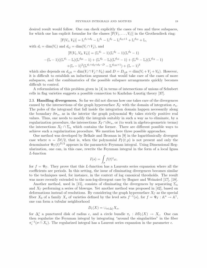
desired result would follow. One can check explicitly the cases of two and three subspaces,for which one has explicit formulae for the classes [F(V1, . . . , Vℓ)] in the Grothendieck ring:

[F(V1, V2)] = Ld1+d2 − Ld1 − Ld2 − Ld12+1 + Ld12 + L,

with di = dim(Vi) and dij = dim(Vi ∩ Vj), and

[F(V1, V2, V3)] = (Ld1 − 1)(Ld2 − 1)(Ld3 − 1)

−(L− 1)((Ld1 − L)(Ld23 − 1) + (Ld2 − L)(Ld13 − 1) + (Ld3 − L)(Ld12 − 1)

+(L− 1)2(Ld1+d2+d3−D − Ld123+1) + (L− 1)3

which also depends on dijk = dim(Vi ∩Vj ∩Vk) and D = Dijk = dim(Vi + Vj + Vk). However,it is difficult to establish an induction argument that would take care of the cases of moresubspaces, and the combinatorics of the possible subspace arrangements quickly becomesdifficult to control.

A reformulation of this problem given in [4] in terms of intersections of unions of Schubertcells in flag varieties suggests a possible connection to Kazhdan–Lusztig theory [37].

2.3. Handling divergences. So far we did not discuss how one takes care of the divergencescaused by the intersections of the graph hypersurface XΓ with the domain of integration σn.The poles of the integrand that fall inside the integration domain happen necessarily alongthe boundary ∂σn, as in the interior the graph polynomial ΨΓ takes strictly positive realvalues. Thus, one needs to modify the integrals suitably in such a way as to eliminate, by aregularization procedure, the intersections XΓ∩∂σn, or (to work in algebro-geometric terms)the intersections XΓ ∩ Σn which contains the former. There are different possible ways toachieve such a regularization procedure. We mention here three possible approaches.

One method was developed by Belkale and Brosnan in [9] in the logarithmically divergentcase where n = Dℓ/2, that is, when the polynomial PΓ(t, p) is not present and only the

denominator ΨΓ(t)D/2 appears in the parametric Feynman integral. Using Dimensional Reg-ularization, one can, in this case, rewrite the Feynman integral in the form of a local IgusaL-function

I(s) =

∫

σf(t)sω,

for f = ΨΓ. They prove that this L-function has a Laurents series expansion where all thecoefficients are periods. In this setting, the issue of eliminating divergences becomes similarto the techniques used, for instance, in the context of log canonical thresholds. The resultwas more recently extended to the non-log-divergent case by Bogner and Weinzierl [17], [18].

Another method, used in [15], consists of eliminating the divergences by separating Σn

and XΓ performing a series of blowups. Yet another method was proposed in [42], based ondeformations instead of resolutions. By considering the graph hypersurface XΓ as the specialfiber X0 of a family Xs of varieties defined by the level sets f−1(s), for f = ΨΓ : An → A1,one can form a tubular neighborhood

Dǫ(X) = ∪s∈∆∗ǫXs,

for ∆∗ǫ a punctured disk of radius ǫ, and a circle bundle πǫ : ∂Dǫ(X) → Xǫ. One can

then regularize the Feynman integral by integrating “around the singularities” in the fiberπ−1

ǫ (σ ∩Xǫ). The regularized integral has a Laurent series expansion in the parameter ǫ.

20 MATILDE MARCOLLI

In general, as we discuss at length below, a regularization procedure for Feynman integralsreplaces a divergent integral with a function of some regularization parameters (such as thecomplexified dimension of DimReg, or the deformation parameter ǫ in the example hereabove) in which the resulting function has a Laurent series expansion around the pole thatcorresponds to the divergent integral originally considered. One then uses a procedure ofextraction of finite values to eliminate the polar parts of these Laurent series in a way thatis consistent over graphs, that is, a renormalization procedure. We therefore turn now torecalling how renormalization can be formulated geometrically, using the results of Connes–Kreimer, as this will be the step relating the “bottom-up” approach to Feynman integralsand motives discussed so far, to the top down approach developed in [25], [26], [27], [28].

3. The Connes–Kreimer theory

We give here a very brief overview of the main results of the Connes–Kreimer theory,as they form the basis upon which the “top-down” approach to understanding the relationbetween quantum field theory and motives rests.

3.1. The BPHZ renormalization procedure. The main steps of what is known in thephysics literature as the Bogolyubov–Parashchuk–Hepp–Zimmermann procedure (BPHZ) aresummarized as follows. (For more details the reader is invited to look at Chapter 1 on [28]).

Step 1: Preparation: one replaces the Feynman integral U(Γ) of (6) by the expression

(18) R(Γ) = U(Γ) +∑

γ∈V(Γ)

C(γ)U(Γ/γ).

Here we suppress the dependence on z, µ and the external momenta p for simplicity ofnotation. The expression (18) is to be understood as a sum of Laurent series in z, dependingon the extra parameter µ. The sum is over the set V(Γ) all proper subgraphs γ ⊂ Γ with theproperty that the quotient graph Γ/γ, where each component of γ is shrunk to a vertex, isstill a Feynman graph of the theory. The main result of BPHZ is that the coefficient of poleof R(Γ) is local.

Step 2: Counterterms: These are the expressions by which the Lagrangian needs to bemodified to cancel the divergence produced by the graph Γ. They are defined as the polarpart of the Laurent series R(Γ),

C(Γ) = −T (R(Γ)).

Here T denotes the operator of projection onto the polar part of a Laurent series.

Step 3: Renormalized value: One then extracts a finite value from the integral U(Γ)by removing the polar part, not of U(Γ) itself but of its preparation:

R(Γ) = R(Γ) + C(Γ)

= U(Γ) + C(Γ) +∑

γ∈V(Γ)

C(γ)U(Γ/γ)

A very nice conceptual understanding of the BPHZ renormalization procedure with theDimReg+MS regularization was obtained by Connes and Kreimer [23], [24], based on areformulation of the BPHZ procedure in geometric terms.


3.2. Renormalization, Hopf algebras, Birkhoff factorization. The first step in thegeometric theory of renormalization is the understanding that the combinatorics of Feynmangraphs of a given theory is governed by an algebraic structure, which accounts for the book-keeping of the hierarchy of subdivergences that occur in multi-loop Feynman integrals. Theright mathematical structure that describes their interactions is a Hopf algebra. This wasfirst formulated by Kreimer [39] as a Hopf algebra of rooted trees decorated by Feynmandiagrams, and then by Connes–Kreimer [23], [24] more directly in the form of a Hopf algebraof Feynman diagrams.

The Connes–Kreimer Hopf algebra ([23]) H = H(T ) depends on the choice of the physicaltheory, in the sense that it involves only graphs that are Feynman graphs for the specifiedLagrangian L(φ). As an algebra it is the free commutative algebra with generators the 1PIFeynman graphs Γ of the theory. It is graded, by loop number, or by the number of internallines,

deg(Γ1 · · ·Γn) =∑

i

deg(Γi), deg(1) = 0.

This grading corresponds to the order in the perturbative expansion.The coproduct already reveals a close relation to the BPHZ formulae. It is given on

generators by

∆(Γ) = Γ⊗ 1 + 1⊗ Γ +∑

γ∈V(Γ)

γ ⊗ Γ/γ,

where the sum is over proper subgraphs γ ⊂ Γ in a specific class V(Γ) determined by theproperty that the quotient graph Γ/γ is still a 1PI Feynman graph of the theory and thatγ itself is a disjoint union of 1PI Feynman graphs of the theory. Unlike Γ which is assumedconnected, the subgraphs γ can have multiple connected components, in which case thequotient graph Γ/γ is the one obtained by shrinking each component to a single vertex.

The antipode is defined inductively by

S(X) = −X −∑

S(X ′)X ′′,

where X is an element with coproduct ∆(X) = X ⊗ 1 + 1⊗X +∑

X ′ ⊗X ′′, where all theX ′ and X ′′ have lower degrees.

We only recalled how the Connes–Kreimer Hopf algebra is constructed for scalar fieldtheories. Recently, van Suijlekom showed [49], [50], [51] how to extend it to gauge theories,icorporating Ward identities as Hopf ideals.

A commutative Hopf algebra H is dual to an affine group scheme G, defined by algebrahomomorphisms

G(A) = Hom(H, A),

for any commutative unital algebra A. In the case of the Connes–Kreimer Hopf algebra thisG is called the group of diffeographisms of the physical theory T and it was proved in [23]that it acts by local diffeomorphisms on the coupling constants of the theory.

The complex Lie group G(C) of complex points of the affine group scheme G, defined asG(C) = Hom(H, C), is a pro-unipotent Lie group. For such groups, which are dual to gradedconnected Hopf algebras that are finite dimensional in each degree, Connes and Kreimerproved by a recursive formula that is is always possible to have a multiplicative Birkhoff

22 MATILDE MARCOLLI

factorization

γ(z) = γ−(z)−1γ+(z)

of loops γ : ∆∗ → G, defined on an infinitesimal disk ∆∗ around the origin in C∗, in termsof two holomorphic functions γ±(z) respectively defined on ∆ and on P1(C) r 0. Thefactorization is unique upon fixing a normalization condition γ−(∞) = 1. Notice that suchBirkhoff factorizations do not always exist for other kinds of complex Lie groups, as onecan see in the example of GLn(C) where the existence of holomorphic vector bundles on theRiemann sphere is an obstruction.

In Hopf algebra terms, one can describe a loop γ : ∆∗ → G(C) on an infinitesimal punctureddisk ∆∗ as an algebra homomorphism φ ∈ Hom(H, C(z)) with values in the field of germs ofmeromorphic functions (covergent Laurent series). The two terms γ+ and γ− of the Birkhofffactorization are, respectively, algebra homomorphisms φ+ ∈ Hom(H, Cz) to convergentpower series, and φ− ∈ Hom(H, C[z−1]). The BPHZ recursive formula is then reformulatedin [23] [24] as the Birkhoff factorization applied to the loop φ(Γ) = U(Γ) given by thedimensionally regularized unrenormalized Feynman integrals. In fact, the recursive formulaof Connes and Kreimer for the Birkhoff factorization can be written as

φ−(X) = −T (φ(X) +∑

φ−(X ′)φ(X ′′)),

for ∆(X) = X⊗1+1⊗X +∑

X ′⊗X ′′, and with T the projection onto the polar part of theLaurent series, and φ+(X) = φ(X) + φ−(X). The fact that the φ± obtained in this way arestill algebra homomorphism depends on the fact that the projection onto the polar part ofLaurent series is a Rota–Baxter operator. In fact, this renormalization procedure by Birkhofffactorization was easily generalized in [31], [32] to arbitrary algebra homomorphisms φ ∈Hom(H,A) from a commutative graded connected Hopf algebra to a Rota–Baxter algebra.When one applies this formula to φ(Γ) = U(Γ) one finds the BPHZ formula with φ−(Γ) =C(Γ) the counterterms and φ+(Γ)|z=0 = R(Γ) the renormalized values.

Notice how, from this point of view, the algebro-geometric Feynman rules discussed above,correspond to the data of a Hopf algebra homomorphism φ ∈ Hom(H,FK) or, in the motiviccase, φ ∈ Hom(H,K0(VK)), together with the assignment of the propagator U(L) = L. Itwould therefore be interesting to know if the rings FK and K0(VK) have a non-trivial Rota–Baxter structure.

4. A top-down approach via Galois theory

As we mentioned earlier, the “top-down” approach to the question of Feynman integralsand periods of mixed Tate motives consists of comparing categorical structures, instead oflooking at varieties and motives associated to individual Feynman graphs. The main idea,developed in my joint work with Connes in [25], [26], [27], [28], is to show that the dataof perturbative renormalization can be reformulated in terms of a Tannakian category ofequivalence classes of differential systems with irregular singularities.

A neutral Tannakian category C is an abelian category, which is k-linear for some field k,has a rigid tensor structure and a fiber functor ω : C → V ectk, which is a faithful exact tensorfunctor to the category of vector spaces over the same field k.


Tannakian categories are extremely rigid structures, namely such a category is equivalentto a category of finite dimensional linear representations of an affine group scheme,

C ≃ RepG.

The affine group scheme G is reconstructed from the category as the invertible natural trans-formations of the fiber functor.

Thus, in order to relate two sets of objects of a seemingly very different nature, of whichone is known (as is the case for mixed Tate motives over a number field) to form a Tannakiancategory, it suffices to show that the other set of objects can also be organized in a similarway, and check that the resulting affine group schemes are isomorphic: this gives then anequivalence of categories. This is precisely what is done in the results of [25].

The reason why this does not yet give an answer to the conjecture lies in the fact thatone only obtains in this way a non-canonical identification, which cannot therefore be usedto explicitly match Feynman integrals to mixed Tate motives. There are other mysteriousaspects, for instance the category of mixed Tate motives involved in the result of [25] is notover Q or Z, but over the ring Z[i][1/2], while all the varieties XΓ involved in the parametricformulation of Feynman integrals are defined over Z. Relating explicitly the top-down ap-proach described below to the bottom-up approach is still an important missing ingredient inthe geometric theory of renormalization, which may possibly provide the key to completinga proof of the main conjecture.

The main results of [25], [26], [27] are summarized as follows.

• Step 1: Counterterms as iterated integrals. One writes the negative piece γ−(z) ofthe Birkhoff factorization as an iterated integral depending on a single element β inthe Lie algebra Lie(G) of the affine group scheme dual to the Connes–Kreimer Hopfalgebra. This is a way of formulating what is known in physics as the ’t Hooft–Grossrelations, that is, the fact that counterterms only depend on the beta function of thetheory (the infinitesimal generator of the renormalization group flow).

• Step 2: From iterated integrals to solutions of irregular singular differential equations.

The iterated integrals obtained in the first step are uniquely solutions to certain dif-ferential equations. This makes it possible to classify the divergences of quantum fieldtheories in terms of families of differential systems with singularities. The fact that, bydimensional analysis, counterterms are independent of the energy scale correspondsin these geometric terms to the flat singular connections describing the differentialsystems satisfying a certain equisingularity condition.

• Step 3: Equisingular vector bundles. Instead of working with equisingular connectionsin the context of principal G-bundles, one can formulate things equivalently in termsof linear representations and of flat connections on vector bundles. These data canthen be organized in a neutral Tannakian category E which is independent of G andtherefore universal for all physical theories.

• Step 4: The Galois group. The Tannakian category of flat equisingular connectionsis equivalent to a category of representations E ≃ RepU∗ of an affine groups schemeU∗ = U ⋊ Gm, where U is the prounipotent affine group scheme dual to the Hopfalgebra HU = U(L)∨, where L = F(e−n;n ∈ N) is the free graded Lie algebra withone generator in each degree.

24 MATILDE MARCOLLI

• Step 5: Motivic Galois group. The same group U∗ = U ⋊ Gm is known to arise (up toa non-canonical identification) as the motivic Galois group of the category of mixedTate motives over the scheme S = Spec(Z[i][1/2]), by a result of Deligne–Goncharov.

We describe briefly each of these steps below.

4.1. Counterterms as iterated integrals. In the Birkhoff factorization, there is in facta dependence on a mass scale µ, inherited from the same dependence of the dimensionallyregularized Feynman integrals Uµ(Γ), so that we have

γµ(z) = γ−(z)−1γµ,+(z),

where one knows by reasons of dimensional analysis that the negative part is independent ofµ. This part is written as a time ordered exponential

γ−(z) = Te−1z

R

∞

0θ−t(β)dt = 1 +

∞∑

n=1

dn(β)

zn,

where

dn(β) =

∫

s1≥s2≥···≥sn≥0θ−s1(β) · · · θ−sn(β)ds1 · · · dsn,

and where β ∈ Lie(G) is the beta function, that is, the infinitesimal generator of renormal-ization group flow, and the action θt is induced by the grading of the Hopf algebra by

θu(X) = unX, for u ∈ Gm, and X ∈ H, with deg(X) = n,

with generator the grading operator Y (X) = nX. This result follows from the analysis of therenormalization group in the Connes–Kreimer theory given in [23] [24], with the recursiveformula for the coefficients dn explicitly solved to give the time ordered exponential above.

The loop γµ(z) that collects all the unrenormalized values Uµ(Γ) of the Feynman integralssatisfies the scaling property

(19) γetµ(z) = θtz(γµ(z))

in addition to the property that its negative part is independent of µ,

(20)∂

∂µγ−(z) = 0.

The Birkhoff factorization is then written in [25] in terms of iterated integrals as

γµ,+(z) = Te−1z

R

−z log µ0 θ−t(β)dt θz log µ(γreg(z)).

Thus γµ(z) is specified by β up to an equivalence given by the regular term γreg(z). Theequivalence corresponds to “having the same negative part of the Birkhoff factorization”.

4.2. From iterated integrals to differential systems. The second step of the argument

of [25] goes as follows. An iterated integral (or time-ordered exponential) g(b) = TeR ba

α(t)dt

is the unique solution of a differential equation dg(t) = g(t)α(t)dt with initial conditiong(a) = 1. In particular, given the differential field (K = C(z), δ) and an affine groupscheme G, and the logarithmic derivative

G(K) ∋ f 7→ D(f) = f−1δ(f) ∈ LieG(K),


one can consider differential equations of the form D(f) = ω, for a flat LieG(C)-valuedconnection ω, singular at z = 0 ∈ ∆∗. The existence of solutions is ensured by the conditionof trivial monodromy on ∆∗

M(ω)(ℓ) = TeR 10

ℓ∗ω = 1, ℓ ∈ π1(∆∗).

These differential systems can be considered up to the gauge equivalence relation of D(fh) =Dh + h−1Df h, for a regular h ∈ Cz. The gauge equivalence is the same thing as therequirement considered above that the solutions have the same negative piece of the Birkhofffactorization,

ω′ = Dh + h−1ωh ⇔ fω− = fω′

− ,

where D(fω) = ω and D(fω′

) = ω′.

4.3. Flat equisingular connections. The third step of [25] consists of reformulating thedata of the loops γµ(z) up to the equivalence of having the same negative piece of the Birkhofffactorization in terms of gauge equivalence classes of differential systems as above. The pointhere is that one keeps track of the µ-dependence and of the way γµ(z) scales with µ and thefact that the negative part of the Birkhoff factorization is independent of µ, as in (19), (20).In geometric terms these conditions are reformulated in [25] as properties of connections on aprincipal G-bundle P = B×G over a fibration Gb → B → ∆, where z ∈ ∆ is the complexifieddimension of DimReg and the fiber µz ∈ Gm over z corresponds to the changing mass scale.The multiplicative group acts by

u(b, g) = (u(b), uY (g)) ∀u ∈ Gm.

The two conditions (19) and (20) correspond to the properties that the flat connection onP ∗ is equisingular, that is, it satisfies:

• Under the action of u ∈ Gm the connection transforms like

(z, u(v)) = uY ((z, u)).

• If γ is a solution in G(C(z)) of the equation Dγ = , then the restrictions alongdifferent sections σ1, σ2 of B with σ1(0) = σ2(0) have “the same type of singularities”,namely

σ∗1(γ) ∼ σ∗

2(γ),

where f1 ∼ f2 means that f−11 f2 ∈ G(Cz), regular at zero.

4.4. Flat equisingular vector bundles. The fourth step of [25] consists of transformingthe information obtained above from equivalence classes of flat equisingular connections onthe principal G-bundle P to a category E of flat equisingular vector bundles. This is possi-ble without losing any amount of information, since the affine group scheme G dual to theConnes–Kreimer Hopf algebra of Feynman graphs of a given physical theory is completely de-termined by its category RepG of finite dimensional linear representations. Thus, consideringall possible flat equisingular vector bundles gives rise to a category that in particular containsas a subcategory the vector bundles that come from finite dimensional representations of G,for any G associated to a particular physical theory, while in itself the category E does notdepend on any particular G, so it is therefore universal for different physical theories.

The category E of flat equisingular vector bundles is defined in [25] as follows.

26 MATILDE MARCOLLI

The objects Obj(E) are pairs Θ = (V, [∇]), where V is a finite dimensional Z-graded vectorspace, out of which one forms a bundle E = B × V . The vector space has a filtrationW−n(V ) = ⊕m≥nVm induced by the grading and a Gm action also coming from the grading.The class [∇] is an equivalence class of equisingular connections, which are compatible withthe filtration, trivial on the induced graded spaces GrW

−n(V ), up to the equivalence relationof W -equivalence. This is defined by T ∇1 = ∇2 T for some T ∈ Aut(E) which iscompatible with filtration and trivial on GrW

−n(V ). Here the condition that the connections∇ are equisingular means that they are Gm-invariant and that restrictions of solutions tosections of B with the same σ(0) are W -equivalent. The morphisms HomE(Θ,Θ′) are linearmaps T : V → V ′ that are compatible with grading, and such that on E ⊕ E′ the followingconnections are W -equivalent:

(

∇′ 00 ∇

)

W−equiv≃

(

∇′ T∇−∇′T0 ∇

)

.

4.5. The Riemann–Hilbert correspondence. Finally, we proved in [25] that the categoryE is a Tannakian category

E ≃ RepU∗ , with U∗ = U ⋊ Gm,

where U is dual, under the relation U(A) = Hom(HU, A), to the Hopf algebra HU = U(L)∨

dual (as Hopf algebra) to the universal enveloping algebra of the free graded Lie algebraL = F(e−1, e−2, e−3, · · · ). The renormalization group rg : Ga → U is a 1-parameter subgroupwith generator e =

∑∞n=1 e−n. In particular, the morphism U → G that realizes the finite

dimensional linear representations of G with equisingular connections as a subcategory of Eis given by mapping the generators e−n 7→ βn to the n-th graded piece of the beta functionof the theory, seen as an element β =

∑

n βn in the Lie algebra Lie(G). There are universalcounterterms in U∗ given in terms of a universal singular frame

γU(z, v) = Te−1z

R v0 uY (e)du

u .

For Θ = (V, [∇]) in E there exists unique ρ ∈ RepU∗ such that

Dρ(γU)W−equiv≃ ∇.

This same affine group scheme U∗ appears in the work of Deligne–Goncharov as the motivicGalois group of the category of mixed Tate motives MS ≃ RepU∗ , with S = Spec(Z[i][1/2]),albeit up to a non-canonical identification. This leads to an identification (non-canonically)of the category E , which by the previous steps classifies the data of the counterterms inperturbative renormalization, with the category MS of mixed Tate motives.

Cartier conjectured [21] the existence of a Galois group acting on the coupling constants ofthe physical theories and related both to the groups of diffeographisms of the Connes–Kreimertheory and to the symmetries of multiple zeta values, and he referred to it as a cosmic Galois

group. In this sense the result of [25] is a positive answer to Cartier’s conjecture, whichidentifies his cosmic Galois group with the affine group scheme U∗ = U ⋊ Gm.


5. The geometry of Dim Reg

We end this exposition with a brief discussion on the subject of Dimensional Regularization.In physics this is taken to mean a formal extension of the rules of integration of Gaussiansby setting

∫

e−λt2dzt := πz/2λ−z/2,

for z ∈ C∗. This prescription can then be used to make sense of a larger set of integrations incomplexified dimension z, which can be reduced to this Gaussian form by the use of Schwingerparameters. However, no attempt is made to make sense of an actual geometry in complexifieddimension z ∈ C∗. We argue here that there are (at least) two possible approaches that canbe used to make sense of spaces in dimension z compatibly with the prescription for theGaussian integration. One is based on noncommutative geometry and it was proposed firstin the unpublished work [29] and later included in our book [28], while the second approachis based on motives and was proposed in [42]. The noncommutative geometry approach isbased on the idea of taking a product, in the sense of metric noncommutative spaces (spectraltriples) of the spacetime manifold over which the quantum field theory is constructed bya noncommutative space Xz whose dimension spectrum (the most sophisticated notion ofdimension in noncommutative geometry) is given by a single point z ∈ C∗. The motivicapproach is based also on taking a product, but this time of the motive associated to anindividual Feynman graph by a projective limit of logarithmic motives Log∞.

In both cases the main idea is to deform the geometry by taking a product of the originalgeometry on which the computation of the un-regularized Feynman integral was performedby a new space, either noncommutative or motivic, which accounts for the shift of z indimension. Recently there has been a considerable amount of activity in relating noncom-mutative geometry and motives (see [22] and [28]). It would be interesting to see if, in thiscontext, there is a way to combine these two approaches to the geometry of DimensionalRegularization.

5.1. The noncommutative geometry of DimReg. The notion of metric space in non-commutative geometry is provided by spectral triples. These consist of data of the formX = (A,H,D), with A an associative involutive algebra represented as an algebra of boundedoperators on a Hilbert space H, together with a self-adjoint operator D on H, with compactresolvent, and with the property that the commutators [a,D] are bounded operators on H,for all a ∈ A. This structure generalizes the data of a compact Riemannian spin manifold,with the (commutative) algebra of smooth functions, the Hilbert space of square integrablespinors and the Dirac operator. It makes sense, however, for a wide range of examples thatare not ordinary manifolds, such as quantum groups, fractals, noncommutative tori, etc. Forsuch spectral triples there are various different notions of dimension. The most sophisticatedone is the dimension spectrum which is not a single number but a subset of the complex planeconsisting of all poles of the family of zeta functions associated to the spectral triple,

Dim = s ∈ C|ζa(s) = Tr(a|D|−s) have poles .

These are points where one has a well defined integration theory on the non-commutativespace, the analog of a volume form, given in terms of a residue for the zeta functions. It isshown in [29], [28] that there exists a (type II) spectral triple Xz with the properties that

28 MATILDE MARCOLLI

the dimension spectrum is Dim = z and that one recoves the DimReg prescription for theGaussian integration in the form

Tr(e−λD2z ) = πz/2λ−z/2.

The operator Dz is of the form Dz = ρ(z)F |Z|1/z , where Z = F |Z| is a self-adjoint operator

affiliated to a type II∞ von Neumann algebra N and ρ(z) = π−1/2(Γ(1 + z/2))1/z , with thespectral measure Tr(χ[a,b](Z)) = 1

2

∫

[a,b] dt, for the type II trace. The ordinary spacetime

over which the quantum field theory is constructed can itself be modeled as a (commutative)spectral triple

X = (A,H,D) = (C∞(X), L2(X,S), /DX)

and one can take a product X ×Xz given by the cup product of spectral triples (adapted totype II case)

(A,H,D) ∪ (Az,Hz,Dz) = (A⊗Az,H⊗Hz,D ⊗ 1 + γ ⊗Dz).

This agrees with what is usually described in physics as the Breitenlohner–Maison prescriptionto resolve the problem of the compatibility of the chirality γ5 operator with the DimRegprocedure, [19]. The Breitenlohner–Maison prescription consists of changing the usual Diracoperator to a product, which is indeed of the form as in the cup product of spectral triples,

D ⊗ 1 + γ ⊗Dz.

It is shown in [29] and [28] that an explicit example of space Xz that can be used to performDimensional Regularization geometrically can be constructed from the adele class space,the noncommutative space underlying the spectral realization of the Riemann zeta functionin noncommutative geometry (see e.g. [22]), by taking the crossed product of the partiallydefined action

N = L∞(Z× R∗) ⋊ GL1(Q)

and the trace

Tr(f) =

∫

Z×R∗

f(1, a) da,

with the operator

Z(1, ρ, λ) = λ, Z(r, ρ, λ) = 0, r 6= 1 ∈ Q∗.

5.2. The motivic geometry of DimReg. We now explain briefly the motivic approach toDimensional Regularization proposed in [42]. The Kummer motives are simple examples ofmixed Tate motives, given by the extensions

M = [u : Z→ Gm] ∈ Ext1DM(K)(Q(0), Q(1))

with u(1) = q ∈ K∗ and the period matrix(

1 0log q 2πi

)

.

These can be combined in the form of the Kummer extension of Tate sheaves

K ∈ Ext1DM(Gm)(QGm(0), QGm(1)),

QGm(1)→ K → QGm(0)→ QGm(1)[1].


The logarithmic motives Logn = Symn(K) are defined as symmetric products of this exten-sion, [6] [35]. They form a projective system and one can take the limit as a pro-motive

Log∞ = lim←−n

Logn.

This corresponds to the period matrix

1 0 0 · · · 0 · · ·log(s) (2πi) 0 · · · 0 · · ·log2(s)

2! (2πi) log(s) (2πi)2 · · · 0 · · ·...

...... · · ·

... · · ·logn(s)

n! (2πi) logn−1(s)(n−1)! (2πi)2 logn−2(s)

(n−2)! · · · (2πi)n−1 · · ·...

...... · · ·

... · · ·

The graph polynomials ΨΓ associated to Feynman graphs define motivic sheaves

MΓ = (ΨΓ : An r XΓ → Gm, Σn r (XΓ ∩ Σn), n − 1, n − 1),

viewed as objects (f : X → S, Y, i, w) in Arapura’s category of motivic sheaves, [5].Then the procedure of Dimensional Regularization can be see as taking a product MΓ ×

Log∞ in the Arapura category of the motivic sheaf MΓ by the logarithmic pro-motive. Theproduct in the Arapura category is given by the fibered product

(X1 ×S X2 → S, Y1 ×S X2 ∪X1 ×S Y2, i1 + i2, w1 + w2).

The reason for this identification is that period computations on a fibered products satisfy∫

π∗X1

(ω) ∧ π∗X2

(η) =

∫

ω ∧ f∗1 (f2)∗(η),

where the integration takes place on σ1×Sσ2 with σi ⊂ Xi with boundary ∂σi ⊂ Yi, accordingto the diagram

X1 ×S X2

πX1yyttttt

ttttt

πX2%%

JJJJJJJJJJ

X1f1

%%KKKKKKKKKKK

X2f2

yysssssssssss

S

This leads to writing the dimensionally regularized parametric Feynman integrals (at least inthe log-divergent case where the term PΓ(t, p) is absent) in the Igusa L-function form

∫

σ ΨzΓα

as a period computation on MΓ × Log∞.

Acknowledgement. A large part of what I described in this paper is based on recent jointwork with Paolo Aluffi and on previous joint work with Alain Connes, whom I thank for theiressential contributions to the development of these ideas and results. Although the articlereflects closely the content of the lecture I delivered at the ECM in the summer of 2008,the actual writing was carried out in the winter 2009, during a stay at MSRI: I thank theinstitute for the hospitality and for support. Discussions with Nikolai Reshetikhin and a talk

30 MATILDE MARCOLLI

I gave in Yongbin Ruan’s seminar helped finalizing the form of this exposition. The topicscovered in this survey will appear in extended form in the book [43] based on a course givenat Caltech in the fall 2008.

References

[1] P. Aluffi, Limits of Chow groups, and a new construction of Chern-Schwartz-MacPherson classes. PureAppl. Math. Q. 2 (2006), no. 4, part 2, 915–941.

[2] P. Aluffi, M. Marcolli, Feynman motives of banana graphs, to appear in Communications in NumberTheory and Physics, arXiv:0807.1690.

[3] P. Aluffi, M. Marcolli, Algebro-geometric Feynman rules, arXiv:0811.2514.[4] P. Aluffi, M. Marcolli, Parametric Feynman integrals and determinant hypersurfaces, arXiv:0901.2107.[5] D. Arapura, A category of motivic sheaves, arXiv:0801.0261.[6] J. Ayoub, The motivic vanishing cycles and the conservation conjecture, in “Algebraic Cycles and Mo-

tives”, London Mathematical Society Lecture Note Series, Vol.343, pp.3–54, Cambridge University Press,2007.

[7] A.A.Beilinson, A.B. Goncharov, V.V. Schechtman, A.N. Varchenko, Aomoto dilogarithms, mixed Hodge

structures and motivic cohomology of pairs of triangles on the plane. in “The Grothendieck Festschrift,Vol. I”, pp.135–172, Progr. Math., 86, Birkhauser, 1990.

[8] P. Belkale, P. Brosnan, Matroids, motives, and a conjecture of Kontsevich, Duke Math. Journal, Vol.116(2003) 147–188.

[9] P. Belkale, P. Brosnan, Periods and Igusa local zeta functions. Int. Math. Res. Not. 2003, no. 49, 2655–2670.

[10] F. Bittner, The universal Euler characteristic for varieties of characteristic zero. Compos. Math. 140(2004), no. 4, 1011–1032.

[11] J. Bjorken, S. Drell, Relativistic Quantum Mechanics, McGraw-Hill, 1964, and Relativistic Quantum

Fields, McGraw-Hill, 1965.[12] S. Bloch, Motives associated to graphs, Japan J. Math., Vol.2 (2007) 165–196.[13] S. Bloch, Lectures on mixed motives. Algebraic geometry—Santa Cruz 1995, 329–359, Proc. Sympos.

Pure Math., 62, Part 1, Amer. Math. Soc., 1997.[14] S. Bloch, Motives associated to sums of graphs, arXiv:0810.1313.[15] S. Bloch, E. Esnault, D. Kreimer, On motives associated to graph polynomials, Commun. Math. Phys.,

Vol.267 (2006) 181–225.[16] S. Bloch, D. Kreimer, Mixed Hodge structures and renormalization in physics, arXiv:0804.4399.[17] C. Bogner, S. Weinzierl, Periods and Feynman integrals, arXiv:0711.4863.[18] C. Bogner, S. Weinzierl, Resolution of singularities for multi-loop integrals, arXiv:0709.4092.[19] P. Breitenlohner, D. Maison, Dimensional renormalization and the action principle, Comm. Math. Phys.

Vol.52 (1977) N.1, 11–38.[20] D. Broadhurst, D. Kreimer, Association of multiple zeta values with positive knots via Feynman diagrams

up to 9 loops, Phys. Lett. B, Vol.393 (1997) 403–412.[21] P. Cartier, A mad day’s work: from Grothendieck to Connes and Kontsevich. The evolution of concepts

of space and symmetry. Bull. Amer. Math. Soc. (N.S.) 38 (2001), no. 4, 389–408.[22] A.Connes, C. Consani, M. Marcolli, Noncommutative geometry and motives: the thermodynamics of

endomotives, Advances in Mathematics, Vol.214 (2007) N.2, 761-831.[23] A. Connes, D. Kreimer, Renormalization in quantum field theory and the Riemann–Hilbert problem I. The

Hopf algebra structure of graphs and the main theorem, Comm. Math. Phys., Vol.210 (2000) 249–273.[24] A. Connes, D. Kreimer, Renormalization in quantum field theory and the Riemann-Hilbert problem. II.

The β-function, diffeomorphisms and the renormalization group. Comm. Math. Phys. 216 (2001), no. 1,215–241.

[25] A. Connes, M. Marcolli, Renormalization and motivic Galois theory. International Math. Res. Notices(2004) N.76, 4073–4091.


[26] A. Connes, M. Marcolli, From Physics to Number Theory via Noncommutative Geometry. Part II: Renor-

malization, the Riemann-Hilbert correspondence, and motivic Galois theory, in ”Frontiers in NumberTheory, Physics, and Geometry, II” pp.617–713, Springer Verlag, 2006.

[27] A. Connes, M. Marcolli, Quantum fields and motives, Journal of Geometry and Physics, Volume 56,(2005) N.1, 55–85.

[28] A. Connes, M. Marcolli, Noncommutative Geometry, Quantum Fields, and Motives, Colloquium Publi-cations, Vol.55, American Mathematical Society, 2008.

[29] A. Connes, M. Marcolli, Anomalies, Dimensional Regularization and noncommutative geometry, unpub-lished manuscript, 2005, available at www.its.caltech.edu/ matilde/work.html

[30] P. Deligne, A.B. Goncharov, Groupes fondamentaux motiviques de Tate mixte. Ann. Sci. Ecole Norm.Sup. (4) 38 (2005), no. 1, 1–56.

[31] K. Ebrahimi-Fard, L. Guo, D. Kreimer, Spitzer’s identity and the algebraic Birkhoff decomposition in

pQFT. J. Phys. A 37 (2004), no. 45, 11037–11052.[32] K. Ebrahimi-Fard, J.M. Gracia-Bondia, F. Patras, A Lie theoretic approach to renormalization. Comm.

Math. Phys. 276 (2007), no. 2, 519–549.[33] H. Gillet, C.Soule, Descent, motives and K-theory. J. Reine Angew. Math. 478 (1996), 127–176.[34] A.B. Goncharov, Multiple polylogarithms and mixed Tate motives, arXiv:math/0103059.[35] A.B. Goncharov, Explicit regulator maps on polylogarithmic motivic complexes. in “Motives, polyloga-

rithms and Hodge theory, Part I” (Irvine, CA, 1998), 245–276, Int. Press Lect. Ser., 3, I, Int. Press,Somerville, MA, 2002.

[36] C. Itzykson, J.B. Zuber, Quantum Field Theory, Dover Publications, 2006.[37] D. Kazhdan, G. Lusztig, Schubert varieties and Poincare duality. in “Geometry of the Laplace operator”

pp. 185–203, Proc. Sympos. Pure Math., XXXVI, Amer. Math. Soc. 1980.[38] M. Kontsevich, D. Zagier, Periods. in “Mathematics unlimited—2001 and beyond”, pp.771–808, Springer,

2001.[39] D. Kreimer, On the Hopf algebra structure of perturbative quantum field theories. Adv. Theor. Math.

Phys. 2 (1998), no. 2, 303–334.[40] M. Levine, Mixed motives, Math. Surveys and Monographs, Vol. 57, AMS, 1998.[41] R.D. MacPherson, Chern classes for singular algebraic varieties. Ann. of Math. (2) 100 (1974), 423–432.[42] M. Marcolli, Motivic renormalization and singularities, arXiv:0804.4824.[43] M. Marcolli, Feynman Motives, book in preparation for Imperial College Press/World Scientific.[44] M. Marcolli, A. Rej, Supermanifolds from Feynman graphs, Journal of Physics A, Vol.41 (2008) 315402

(21pp). arXiv:0806.1681.[45] B. Mohar, C. Thomassen, Graphs on Surfaces, Johns Hopkins University Press, 2001.[46] N. Nakanishi, Graph Theory and Feynman Integrals. Gordon and Breach, 1971.[47] M.H. Schwartz, Classes caracteristiques definies par une stratification d’une variete analytique complexe.

I. C. R. Acad. Sci. Paris, Vol.260 (1965) 3262–3264.[48] T. Terasoma, Mixed Tate motives and multiple zeta values. Invent. Math. 149 (2002), no. 2, 339–369.[49] W. van Suijlekom, Renormalization of gauge fields: a Hopf algebra approach. Comm. Math. Phys. 276

(2007), no. 3, 773–798.[50] W. van Suijlekom, The Hopf algebra of Feynman graphs in quantum electrodynamics. Lett. Math. Phys.

77 (2006), N.3, 265–281.[51] W. van Suijlekom, Representing Feynman graphs on BV-algebras, arXiv:0807.0999.[52] V. Voevodsky, Triangulated categories of motives over a field. in “Cycles, transfers, and motivic homology

theories”, pp.188–238, Ann. of Math. Stud., 143, Princeton Univ. Press, 2000.

Documents

FEYNMAN INTEGRALS AND MOTIVESmatilde/ECMpaper.pdf · FEYNMAN INTEGRALS AND MOTIVES MATILDE MARCOLLI and Beyond the Inﬁnite (Stanley Kubrick, 2001 - A Space Odyssey) Contents 1