Ple

ase

note

that

this

is a

n au

thor

-pro

duce

d P

DF

of a

n ar

ticle

acc

epte

d fo

r pub

licat

ion

follo

win

g pe

er re

view

. The

def

initi

ve p

ublis

her-a

uthe

ntic

ated

ver

sion

is a

vaila

ble

on th

e pu

blis

her W

eb s

ite

1

Deep Sea Research Part I: Oceanographic Research Papers November 2007, Volume 54, Issue 11, Pages 1912-1935 http://dx.doi.org/10.1016/j.dsr.2007.06.011 © 2007 Elsevier Ltd All rights reserved.

Archimer Archive Institutionnelle de l’Ifremer

http://www.ifremer.fr/docelec/

Ferromanganese nodule fauna in the Tropical North Pacific Ocean :

species richness, faunal cover and spatial distribution

Julie Veillette1, *, Jozée Sarrazin2, Andrew J. Gooday3, Joëlle Galéron2, Jean-Claude Caprais2, Annick Vangriesheim2, Joël Étoubleau2, James R. Christian4, S. Kim Juniper1, 5

1Centre GÉOTOP, Université du Québec à Montréal, C.P. 8888, Succursale Centre-Ville, Montréal, Québec H3C 3P8, Canada 2Institut Français de Recherche pour l'Exploitation de la MER/ Département Étude des Écosystèmes Profonds, Centre de Brest BP 70, 29280 PLOUZANE, France 3National Oceanography Centre, Southampton, University of Southampton Waterfront Campus, European Way, Southampton, SO14 3ZH, UK 4Fisheries and Oceans Canada, Canadian Centre for Climate Modelling and Analysis, University of Victoria, P.O. Box 1700, Victoria, British Columbia V8W 2Y2, Canada 5Present address : School of Earth and Ocean Sciences, University of Victoria, P.O. Box 3020, Victoria, British Columbia V8W 3N5, Canada *: Corresponding author : Julie Veillette, email address : julie.veillette.2@ulaval.ca

Abstract: The poorly known ferromanganese nodule fauna is a widespread hard substratum community in the deep sea that will be considerably impacted by large-scale nodule mining operations. The objective of this study was to analyze the spatial distribution of the fauna attached to nodules in the Clarion-Clipperton Fracture Zone at two scales; a regional scale that includes the east (14°N, 130°W) and the west (9°N, 150°W) zones and a local scale in which different geological facies (A, B, C and west) are recognizable. The fauna associated with 235 nodules was quantitatively described: 104 nodules from the east zone (15 of facies A, 50 of facies B and 39 of facies C) and 131 nodules from the west zone. Percent cover was used to quantify the extent of colonization at the time of sampling, for 42 species out of the 62 live species observed. Fauna covered up to 18% of exposed nodule surface with an average of about 3%. While species richness increased with exposed nodule surface, both at the regional and at the facies scales (except for facies A), total species density decreased (again except for facies A). When all nodules were included in the statistical analysis, there was no relation between faunal cover and exposed nodule surface. Nevertheless, faunal cover did decrease with exposed nodule surface for the east zone in general and for both facies B and C in particular. Species distributions among facies were significantly different but explained only a very small portion of the variance (not, vert, similar5%). We identified two groups of associated species: a first group of two species and a second group of six species. The other species (34) were independently distributed, suggesting that species interactions play only a minor role in the spatial distribution of nodule fauna. The flux of particulate organic carbon to the bottom is the only major environmental factor considered to vary between the two zones within this study. We conclude that the higher species richness and higher percent faunal cover of the east zone can be partially attributed to greater food availability derived from surface inputs. Moreover, the surfaces of facies B and C nodules had a complex, knobby micro-relief, creating microhabitat heterogeneity that may also have contributed to the greater species richness observed in the east zone. Keywords: Ferromanganese nodules; Fixed fauna; Agglutinated foraminifera; Geographical distribution; Environmental factors; Environmental impacts

4

1. Introduction

Faunas that encrust ferromanganese nodules are poorly known, even though the hard

substratum formed by the nodules is widespread in the deep sea, particularly in the

Pacific Ocean where they may cover more than 50% of the seafloor (Smith and

Demopoulos, 2003; Thistle, 2003). Nodules represent a valuable natural resource.

However, in order for nodule mining to be economically viable, exploitation will

likely be at scales of tens to hundreds of thousands of square kilometres (Glover and

Smith, 2003; Thiel, 2003). Among the potential impacts of nodule mining is the

destruction of the fauna attached to the nodules (Thiel et al., 1993) and the partial

covering of surrounding epifauna by sediment blanketing (Morgan et al., 1999;

Sharma et al., 2001; Thiel et al., 2001). In order to manage and mitigate these

impacts, it is critical that we better understand the composition and distribution of the

nodule fauna and its relationship to the mineral substratum and other environmental

factors.

The study of hard substratum communities in nodule fields has been neglected

compared to adjacent sediment communities, probably because of the difficulties

inherent in remotely sampling nodules from the sea surface. Most previous studies of

nodule faunas focused on their role in nodule formation and growth (Graham and

Cooper, 1959; Ehrlich, 1972; Dudley and Margolis, 1974; Greenslate et al., 1974;

Wendt, 1974; Dudley, 1976; Dugolinsky, 1976; Dugolinsky et al., 1977; Dudley,

5

1978; Thiel, 1978; Bignot and Lamboy, 1980; Riemann, 1983; von Stackelberg,

1984; Riemann, 1985; Thiel et al., 1993). The bacteria associated with nodules

(Ehrlich, 1972; Burnett and Nealson, 1981) and the fauna found within nodule

crevices have been examined (Thiel et al., 1993; Maybury, 1996), but the only

detailed ecological study of organisms living on nodule surface was conducted by

Mullineaux (1987, 1989). Her investigation, which included previously overlooked,

delicate, mat- or net-like foraminiferal taxa that are a major element of these

encrusting assemblages, was based on box core samples from the central (30ºN,

157ºW) and tropical (5ºN, 125ºW) North Pacific. Other deep-sea, hard substratum

communities that have been studied systematically at the same spatial scales

(centimeters-millimeters) as the nodules include sponge stalks (Beaulieu, 2001),

indurated sediment around hydrothermal vents (Jonasson et al., 1995; Jonasson and

Schröder-Adams, 1996), dropstones (Heron-Allen and Earland, 1932; Gooday,

unpublished data), large foraminiferal tests (Gooday and Haynes, 1983), experimental

substrates on seamounts (Bertram and Cowen, 1994) and sunken woods (Turner,

1973). At a larger spatial scale, Tilot (2006a, b) has examined the megafaunal

assemblages of the nodule ecosystem in the tropical North Pacific Ocean.

Several major research programs in the Pacific and Indian Oceans have investigated

the potential impacts of nodule mining. These include: DISCOL (Disturbance and

Recolonization Experiment in a Manganese Nodule Area of the Deep South Pacific

Ocean) (Borowski and Thiel, 1998; Thiel et al., 2001), BIEs (Benthic Impact

6

Experiments) (Sharma et al., 2000; Sharma et al., 2001; Radziejewska, 2002), JET

(Japan Deep-sea Impact Experiment) (Fukushima 1995) and INDEX (Indian Deep-

sea Environment Experiment) (Raghukumar et al., 2001). However, these studies did

not specifically consider the impact of nodule mining on the nodule-dwelling fauna.

The objective of the present study was to improve knowledge of pristine nodule

faunas in order to facilitate environmentally sustainable management of mining

activities. The spatial distribution of the nodule fauna was analyzed at two scales: a

regional scale that includes the east (14°N, 130°W) and the west (9°N, 150°W) zones

and a local scale within which different nodule facies (A, B, C and west) were

recognizable. Water depth was similar in the two zones (varying from 4900 to 5050

m). Four properties of the nodule substratum that could influence faunal distribution

were also examined: nodule size, geochemical composition, morphology and surface

texture. We analyzed the distribution of species among zones and facies, and nodule

groupings using faunal characteristics in order to determine the most influential

factors on faunal spatial distribution. Finally, species assemblages were investigated

as a potential factor structuring faunal distributions on nodules.

The present study extends previous work by Mullineaux (1987, 1989) in several key

respects. First, we carried out a sampling method comparison, comparing results from

nodules obtained with a USNEL box corer with those from nodules scooped up by

the Nautile submersible. Secondly, the large number of nodules sampled at locations

7

that differed from those studied by Mullineaux permitted extensive characterization,

quantification and distribution analysis of nodule fauna. The spatial distribution of the

nodule fauna at the scale of the nodule itself is considered in a separate paper

(Veillette et al., in press).

2. Materials and methods

2.1. Sampling sites

The NODINAUT cruise (RV l’Atalante; May 18th – June 27th 2004) explored and

sampled two geographical zones located in the French mining claim in the tropical

Pacific: the east zone (14°N, 130°W) and the west zone (9°N, 150°W) (Fig. 1). Both

zones are located in the Clarion-Clipperton Fracture Zone at depths varying from

4900 to 5050m. The east zone is located to the north of Mullineaux’s (1987)

equatorial Pacific site. It was previously visited by the NIXONAUT cruise

(November 18th – December 22nd 1988) (Cochonat et al., 1992). Three different

nodule facies were observed in the east zone (A, B and C) where they cover hundreds

of square kilometers. The facies were differentiated according to their general shape,

size, surface morphology of the nodules and the relation between the nodule and its

environment (degree of burial in the sediment, presence of volcanic material)

(Saguez, 1985; Morel and Le Suavé, 1986). Facies A nodules were small spheres

(less than 4 cm diameter) with smooth surfaces and lay at the surface of the sediments

8

on slight slopes. Facies C nodules were the largest (average of 11 cm diameter) but

their sizes varied considerably (from 2 to 15 cm diameter). They appeared as half

buried spheres in the sediments. Knobs and protrusions characterized their smooth-

textured upper region and their sides were rough. Facies B nodules were ovoid,

medium in size (average length 5 cm), most of their surface texture was rough and

they were slightly buried in the sediments. An undescribed facies that characterizes

the west zone is referred to as the “west facies”. These nodules were generally ovoid

but occurred in different shapes. They were small to medium in size (from 2 to 9 cm

in length), their surface texture was rough and they were slightly buried in the

sediments. Even though our visual classification, commonly used by geologists,

appears to be subjective, differences in the geochemical composition of the nodules

from different facies support this approach (Tilot, 1992, 1993; Hoffert and Saget,

2004).

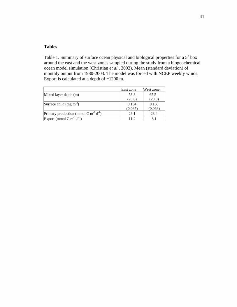
Primary productivity in this region is estimated to be moderate compared to the high

equatorial productivity (DuCastel, 1985; Skornyakova and Murdmaa, 1992; Knoop et

al., 1998). We developed estimates of surface chlorophyll, mixed layer depth,

primary productivity and production export for 5˚ boxes around the east and west

zones, using SeaWiFs ocean color data and numerical modeling. Surface chlorophyll

was slightly higher in the east zone (Fig. 2 and Table 1), as was primary productivity

(Table 1). The greatest difference between the two zones was for export production

(Table 1). While the sedimentation rate in the Clarion-Clipperton Fracture Zone

9

appears to be moderate (Hoffert, pers. comm.), the east zone benefits from a greater

flux of particulate organic carbon to the bottom, likely as a result of longitudinal

advection of organic matter. The east zone lies beneath the North Equatorial Current

and the west zone beneath the North Equatorial Counter Current (DuCastel, 1985;

Smith and Demopoulos, 2003).

Near-bottom currents observed during the NODINAUT cruise (short term ADCP-

WH300 measurements at ten meters above the bottom) were very weak and were of

the same order in the two zones (3.5 – 4 cm s-1). Their direction was toward

east/south-east in the east zone and east/north-east in the west zone meaning that

nodule faunas do not always experience unidirectional currents. There were some

very slight speed and direction variations due to semi-diurnal tidal oscillations.

Previous long-term data (Pujol, 1988; Mauviel, 1990) indicated the existence of

inertial oscillations (2 – 3 days) and longer term oscillations (around 2 – 3 months) of

higher amplitude. According to these data, the current direction encountered during

the NODINAUT cruise was always associated with higher current speeds. We

assume, therefore, that the NODINAUT cruise took place during a period when

current speeds were somewhat higher than normal.

Bottom relief can influence current speed and direction (Morgan et al., 1999). We

attempted to estimate currents at the scale of the nodules at several cm above the

bottom with a modified weathercock but results are too preliminary to be significant.

10

Measured bottom water temperature in both zones was around 1ºC. Seawater

chemical properties measured at the nodule scale (pH, salinity, dissolved oxygen,

alkalinity, dissolved organic carbon (DOC) and nutrients) were also similar in the two

zones.

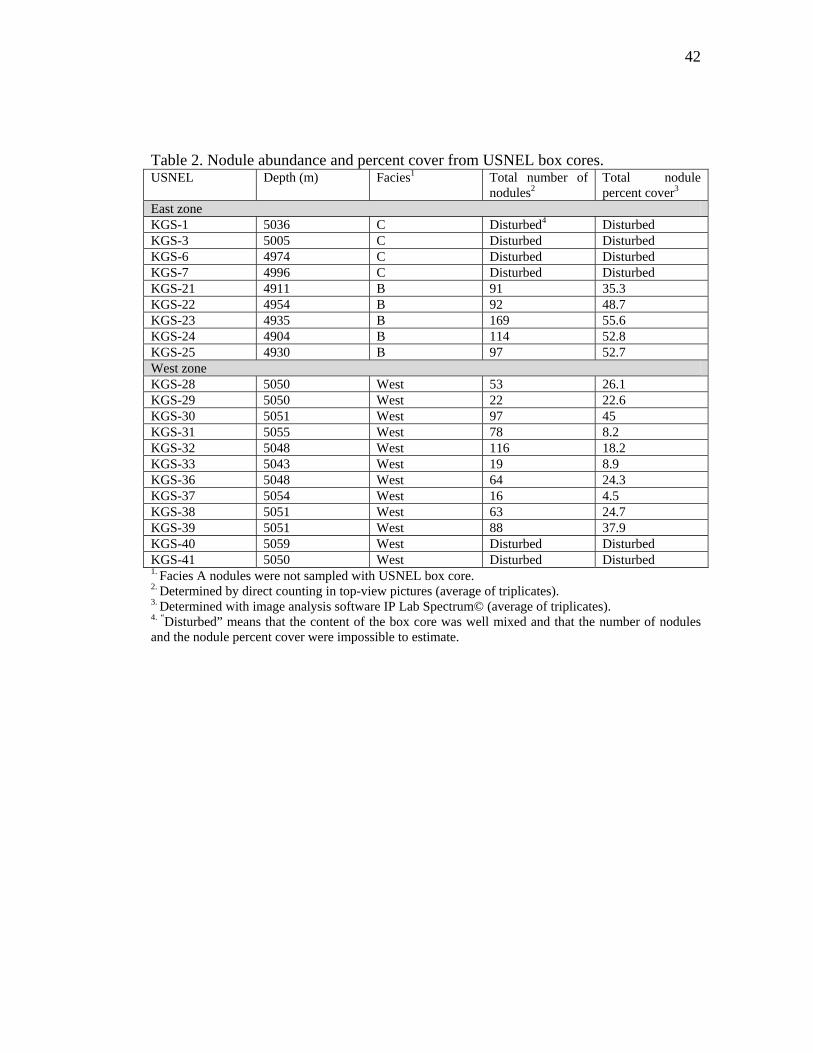
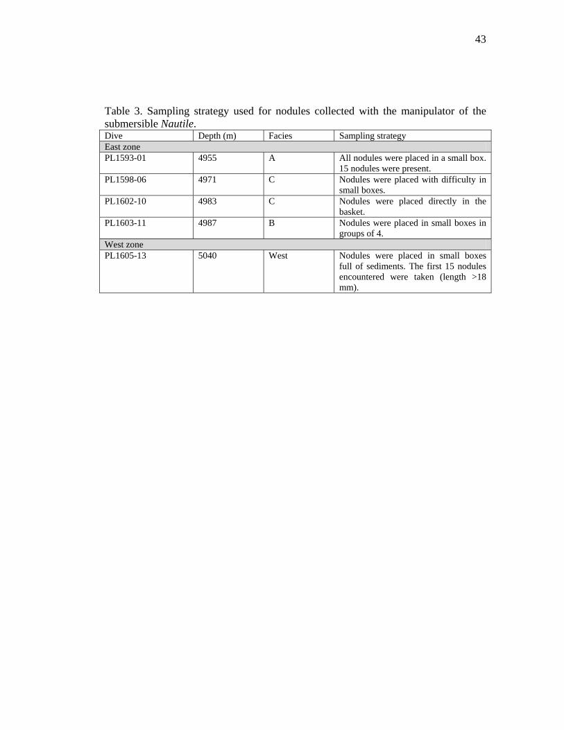
2.2. Sampling methods

Nodules were sampled using either a USNEL box corer (sampled area of 50 X 50 cm)

or the manipulator of the Nautile submersible (Table 2 and 3). A top-view photo of

each USNEL box core was taken before eight randomly chosen nodules were

removed from the sediment and washed carefully with seawater. The sampled

nodules were stored in 4% formaldehyde and transferred to 70% alcohol after several

days. They were all carefully packed for transportation in jars of different sizes.

Plastic packing was placed in the jars to immobilize the nodules. During all

manipulations, nodules were never allowed to dry and were handled with the greatest

care possible because of their high friability.

The two different sampling methods (USNEL box corer versus Nautile submersible)

were compared in order to test the effect of sampling method on our results and on

nodule integrity and fauna. We were particularly interested in whether: 1) the

sampling method influenced the size of the nodules collected; 2) one sampling

method was more destructive than the other, damaging the most fragile living forms

11

and decreasing species richness. The nodule surface above the sediment line was used

as an indicator of nodule size.

2.3. Nodule substratum

Four characteristics of the nodule substratum were considered in relation to faunal

distribution: nodule size, geochemical composition, morphology and texture. The

influence of nodule size on the attached fauna was investigated by testing regressions

of species richness, species density and percent faunal cover in relation to the nodule

surface above the sediment line. For the geochemical composition analysis, the

metallic composition of a nodule cross section from each facies was determined. We

were specifically interested in possible relationships between the fauna and the

geochemical composition of the outer nodule layer. Nodule morphology and texture

are described elsewhere (Veillette et al., in press).

2.4. Nodule surface area determination

Nodule surface area was calculated in order to compare zones and facies. Since

nodule surfaces below the sediment line are rarely colonized, only the area above the

sediment line was considered. This exposed surface area was determined differently

for each facies since the constituent nodules exhibited different morphologies. The

entire surface of facies A nodules could be colonized since they were situated on the

12

sediment surface. For these nodules, the surface area available for colonization was

estimated using the sphere surface formula (4πr2). Facies B and west nodules were

mostly ovoid and buried in the sediment. Their surface area was determined using IP

Lab Spectrum© image analysis software, assuming that top-view photos provided a

good representation of nodule surface area above the sediment line. Facies C nodules

appeared as spheres half buried in the sediment. When the vertical or near vertical

sides of the nodules extended more than 30 mm above the sediment before flattening

to form the upper region, the surface area was separated into top and side. In order to

control for the irregular shape of most nodules, eight measures of the height of the

sides were taken at every 45º around the nodule circumference. When the sides of

facies C nodules were 30 mm or less in height, nodule surface area was determined

using the same methodology as for facies B and west. For nodules greater than 30

mm in side heights, side surface area was calculated using the surface formula for an

open cylinder (height x circumference). All measurements and surface determination

with IP Lab Spectrum© were made in triplicate.

2.5. Faunal identification and quantification

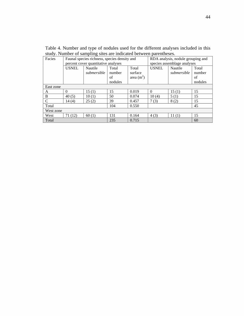
The fauna associated with 235 nodules (greater than 18 mm in length), collected

either by a USNEL box corer or by the Nautile from four different nodule facies, was

described quantitatively (Table 4). The total nodule surface area examined was 0.715

m2. Identification of living organisms on nodule surfaces was done using a binocular

13

dissecting microscope. High power light microscopy and scanning electron

microscopy were also used to examine smaller forms or particular structures and to

determine if unknown forms were protozoans, metazoans or inorganic forms. The

tests of most foraminifera (protozoans) were partially broken in order to determine if

protoplasm was present and therefore whether the organism was alive or dead.

Foraminiferal species that were considered to be alive at the time of collection (based

on the presence of intact protoplasm) were quantified. However, some foraminifera,

for example, komokiacean-like forms in which the test interior is dominated by

stercomata, rarely contained visible protoplasm. In these cases, unbroken tests were

regarded as being live when collected. Despite all precautions taken during handling

of the nodules, some very fragile structures may have been destroyed or lost prior to

identification. Thus, faunal identifications in this study could be biased towards more

robust forms firmly attached to nodule surfaces.

Faunal mats and domes were quantified by their percent cover (Mullineaux, 1987),

whereas upright structures were quantified by their presence/absence.

Presence/absence data were used to calculate species richness, defined as “the

number of species present, without any regard for the exact area or number of

individuals examined” (Hurlbert, 1971). The surface area covered by upright

structures is negligible and thus, the percent cover includes all forms covering the

nodule surface. In order to simplify the faunal cover analysis, every encrusting

14

species was assumed to represent a circle or a rectangle. The dimensions of the

organisms were then measured under a binocular microscope equipped with an

eyepiece scale. For species forming anastomosing networks, percent cover within the

limits of the structure was estimated. Density (number of individuals per unit area)

was not used in this study since the vast majority of the living forms were

foraminifera that were best quantified in terms of percent cover (Mullineaux, 1987).

We recognised two foraminiferal feeding types. Type I included species in which the

test contained cytoplasm and lacked obvious accumulations of stercomata (faecal

pellets). In feeding type II , which included komokiaceans such as Chrondrodapis,

the test contains accumulations of stercomata and the cytoplasm is very sparse.

2.6. Statistical analyses

The quantitative comparison of faunal species richness, species density and percent

cover between zones included all nodules, since the sample sizes of both zones were

relatively similar (neast=104, nwest = 131; Table 4). The non-parametric Mann-Whitney

test was used to test for differences between the two zones because the two main

assumptions for the t-test (homogeneity of variances and normal distributions) were

never met. All nodules were included in the inter-facies comparisons but unbalanced

sample size (nA= 15, nB= 50, nC= 39, nwest= 131; Table 4) was controlled for. Spatial

bias could not be controlled for because of the variation in the number of sampling

15

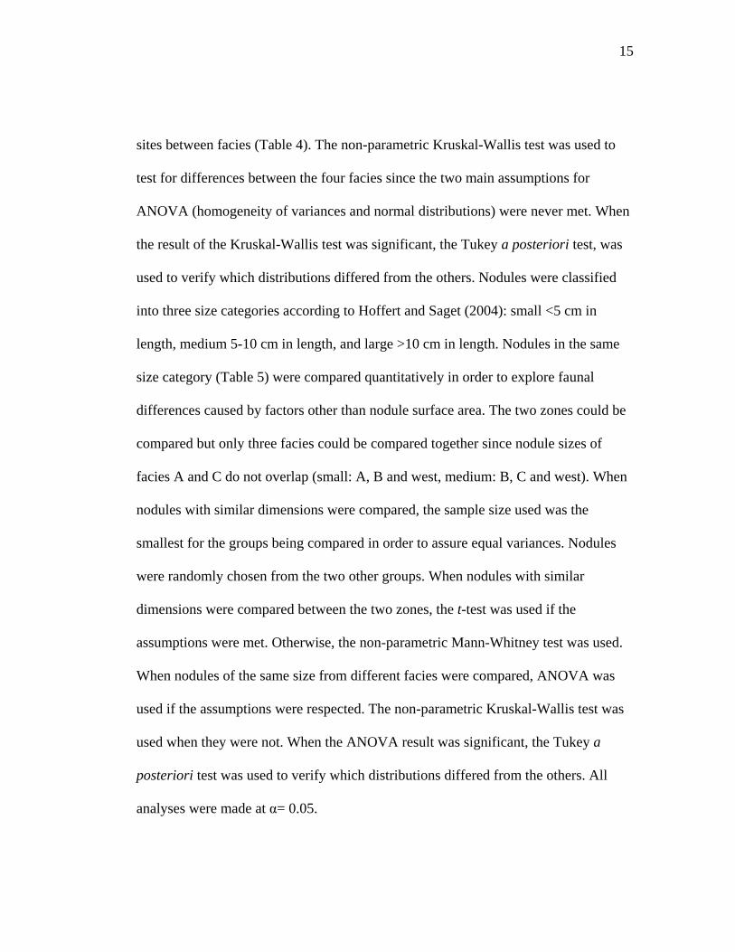
sites between facies (Table 4). The non-parametric Kruskal-Wallis test was used to

test for differences between the four facies since the two main assumptions for

ANOVA (homogeneity of variances and normal distributions) were never met. When

the result of the Kruskal-Wallis test was significant, the Tukey a posteriori test, was

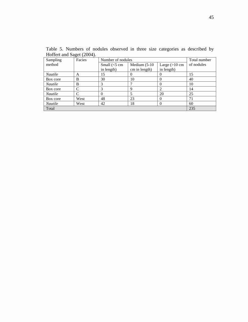
used to verify which distributions differed from the others. Nodules were classified

into three size categories according to Hoffert and Saget (2004): small <5 cm in

length, medium 5-10 cm in length, and large >10 cm in length. Nodules in the same

size category (Table 5) were compared quantitatively in order to explore faunal

differences caused by factors other than nodule surface area. The two zones could be

compared but only three facies could be compared together since nodule sizes of

facies A and C do not overlap (small: A, B and west, medium: B, C and west). When

nodules with similar dimensions were compared, the sample size used was the

smallest for the groups being compared in order to assure equal variances. Nodules

were randomly chosen from the two other groups. When nodules with similar

dimensions were compared between the two zones, the t-test was used if the

assumptions were met. Otherwise, the non-parametric Mann-Whitney test was used.

When nodules of the same size from different facies were compared, ANOVA was

used if the assumptions were respected. The non-parametric Kruskal-Wallis test was

used when they were not. When the ANOVA result was significant, the Tukey a

posteriori test was used to verify which distributions differed from the others. All

analyses were made at α= 0.05.

16

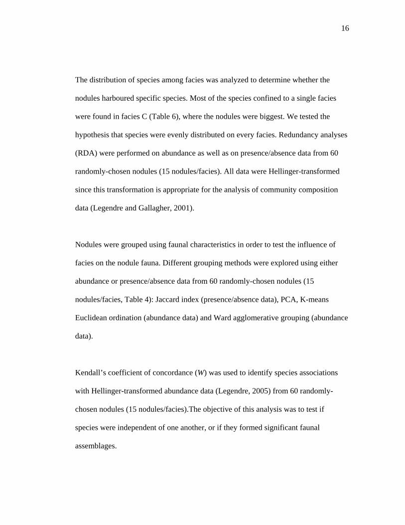
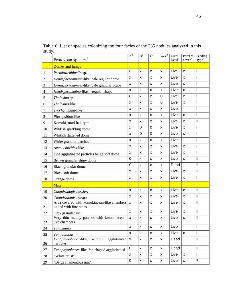
The distribution of species among facies was analyzed to determine whether the

nodules harboured specific species. Most of the species confined to a single facies

were found in facies C (Table 6), where the nodules were biggest. We tested the

hypothesis that species were evenly distributed on every facies. Redundancy analyses

(RDA) were performed on abundance as well as on presence/absence data from 60

randomly-chosen nodules (15 nodules/facies). All data were Hellinger-transformed

since this transformation is appropriate for the analysis of community composition

data (Legendre and Gallagher, 2001).

Nodules were grouped using faunal characteristics in order to test the influence of

facies on the nodule fauna. Different grouping methods were explored using either

abundance or presence/absence data from 60 randomly-chosen nodules (15

nodules/facies, Table 4): Jaccard index (presence/absence data), PCA, K-means

Euclidean ordination (abundance data) and Ward agglomerative grouping (abundance

data).

Kendall’s coefficient of concordance (W) was used to identify species associations

with Hellinger-transformed abundance data (Legendre, 2005) from 60 randomly-

chosen nodules (15 nodules/facies).The objective of this analysis was to test if

species were independent of one another, or if they formed significant faunal

assemblages.

17

3. Results

3.1. Sampling methods

For facies B and C nodules, the two sampling methods yielded different size

distributions (Table 5). The results of the analyses showed that the nodules sampled

with the submersible Nautile were statistically bigger for both facies (Fig. 3). The

dominant species on the nodules sampled by the USNEL box corer and the Nautile

were slightly different, but in general all sampled nodules yielded similar

assemblages of delicate organisms (Table 8A and 8B). The sampling method did not

seem to influence species richness for facies B and C since the species accumulation

curves of the two sampling methods overlapped (Fig. 4). Facies west nodules

collected with the Nautile had lower species richness than those collected with the

USNEL box corer. The number of nodules observed appeared to be sufficient since

all accumulation curves tended towards an asymptote, where the number of new

species observed no longer increased with increasing sample size (Fig. 4). However,

some of these trends [Facies A, B (PL), C (USNEL)] could also be artefacts due to

the small number of observed nodules.

3.2. Nodule faunal composition

18

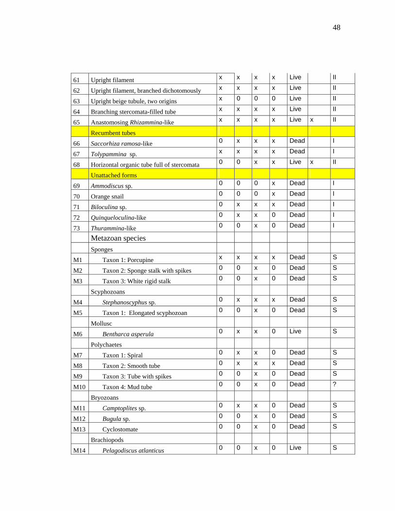
We identified a total of 73 protozoan and 17 metazoan species associated with nodule

surfaces (see “Catalogue of nodule fauna”) (Fig. 5 and Table 6). Eleven protozoan

and 8 metazoan species were identified to species or genus level, the remainder were

indeterminate, i.e. they could not be assigned to any described species or genera. The

protozoans were all foraminifera, with the exception of two probable

xenophyophores. They were all attached directly to the nodule surface except for five

species, which were incorporated into agglutinated mats.

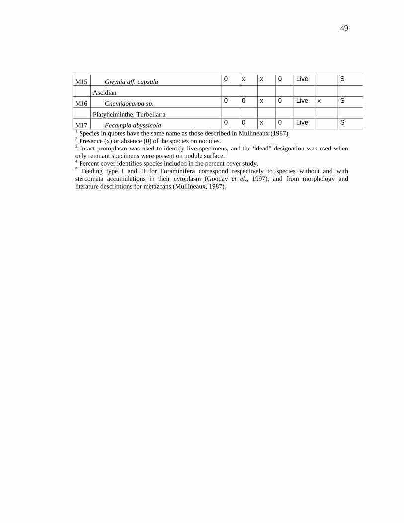
Around 70% (62 out of 90) of the species observed were considered to be living

when collected. However, the proportion was substantially higher for protozoans

(78%) than for metazoans (29%). Only these 62 live species (57 protozoans and 5

metazoans) were included in the species richness analysis. Sixty percent of the

protozoan species represented feeding type I based on the presence of stercomata-free

protoplasm. The remainder (37%) are considered to be feeding type II based on the

accumulation of stercomata within the test (Gooday et al., 1997). All metazoan

species (except “mud tube”) were classified as suspension feeders.

Percent cover was used to quantify the extent of colonization at the time of sampling.

Out of the 62 live species, 41 protozoans (mostly mats, domes and tunnels) and one

metazoan (the ascidian Cnemidocarpa sp.) were quantified by percent cover. Fauna

covered up to 18% of the exposed nodule surface, with a mean of about 3%.

19

3.3. Species richness and density

Species richness per nodule was higher in the east zone than in the west zone (Fig.

6A) even when nodules of the same size were compared (Table 7). Moreover, at the

facies scale, facies C followed by facies B hosted more species than facies A or west

as confirmed by the Tukey test (Fig. 7A). Also, facies B nodules yielded a more

diverse assemblage than facies A or west nodules when only small nodules were

considered (Table 7). On the other hand, facies C nodules were more species rich

than facies B or west nodules when only medium nodules were included in the

analysis (Table 7).

Species density (number of species per mm2) was not significantly higher in the east

zone than in the west zone (Fig. 6B). However, when only small nodules were

considered, species density was higher in the east than in the west zone (Table 7). At

the facies level, facies B had the highest species density, while facies A and west

were not different, and facies C had the lowest species density according to the Tukey

test (Fig. 7B). These rankings still hold when only small nodules were compared but

in this case, facies C was not included (Table 7). For medium nodules, there was no

significant difference in species density between facies B and C, or between facies C

and facies west. However, facies B had a higher species density than facies west

(Table 7).

20

3.4. Percent cover

Percent faunal cover was significantly higher in the east zone than in the west zone

even when the same nodule sizes were compared (Fig. 6C). At the facies scale, facies

B nodules were more heavily encrusted with fauna than facies C, followed by facies

A and west according to the Tukey test (Fig. 7C). These trends remained true for

small nodules only, although in this case, facies C was not included (Table 7).

However, there were no differences in percent cover between facies B, C and west for

medium nodules (Table 7).

3.5. Nodule size

Facies C nodules were larger than facies A, B or west nodules when nodules obtained

using both sampling methods were pooled together (Fig. 3). There was no significant

difference in nodule surface area between facies A, B and west. We examined the

relationship between nodule size and species richness, species density and percent

cover. It might be expected that the number of species would increase with nodule

surface area. Figure 7A shows that the regression between the number of species and

the exposed nodule surface is significant when all nodules are considered (P<0.0001),

at both the regional (east, P<0.0001; west, P<0.0001) and the facies scales (facies B,

P= 0.0310; facies C, P<0.0001), except for facies A (P= 0.1882). These regressions

exhibit positive slopes, as expected. The regressions between species density and

21

exposed nodule surface are significant as well (all, P<0.0001; east, P<0.0001; west,

P=0.0011; facies B, P<0.0001; facies C, P<0.0001), again except for facies A

(P=0.8656) (Fig. 8B). Nevertheless, the slopes of these regressions are negative,

meaning that the number of species per unit surface area decreased with nodule size.

Furthermore, there is no relation between faunal cover and exposed nodule surface

when all nodules are included (P= 0.5219) (Fig. 8C). However, east zone (P<0.0001)

as well as facies B (P=0.0161)and C (P<0.0001) nodules present significant

regressions with negative slopes.

3.6. Species distributions between facies

Tables 8A and 8B show, respectively, the relative abundance of the top ten species in

both zones (Table 8A) and among the four facies studied (Table 8B). Seven species

were abundant in both zones and six species were abundant in every facies. Two

foraminiferal species were observed only on facies A nodules, one foraminiferal

species was only found on facies B, one unattached foraminiferan and ten metazoan

species were noted only on facies C nodules and two unattached forms of

foraminifera only occurred on facies west (Table 6).

For all facies, the redundancy analyses show similar patterns with abundance and

presence/absence data (Fig. 9). Species 1 and 36 seem to be strongly associated with

facies west. Species 22, 23, 45, 19, 28 and 46 were found mostly in the east zone.

22

Although species 28 and 46 were present in every facies, their abundance was much

greater on facies C nodules. However, these trends, although significant (p= 0.0005

and p= 0.0001), explain only a very small portion of the variance of the distribution

of species among facies (R2= 0.054 and R2= 0.063).

3.7. Nodule grouping and species assemblages

Nodule grouping using the Jaccard index method yielded three groups of seven, two

and 49 nodules. Nodules were at most 75% similar. The PCA, K-means Euclidean

ordination and the Ward agglomerative grouping method used abundance data and

yielded similar results. For the PCA, K-means Euclidean ordination, six groups

composed of eight, five, four, two, ten and 26 nodules respectively were formed. The

Ward agglomerative grouping method also formed six groups, containing in this case

nine, two, 20 and three groups, each of eight nodules. The nodules composing these

groups were almost the same ones, irrespective of the method used.

Table 9C shows that two significant groups of associated species exist: one that

includes two species and the other including six species. The remaining 34 species

(out of 42) are independently distributed.

4. Discussion

23

4.1. Sampling methods

There was a bias toward the sampling of larger nodules with the Nautile submersible.

However, the nodule size differences were too slight to explain the observed faunal

differences and nodules collected using both methods were therefore pooled. In future

studies, human bias in the collection of nodules with the submersible could easily be

minimized by using a sampling frame with the same area as that sampled by the box

corer (50 X 50 cm). This frame could be laid out on the sediment surface and nodules

randomly collected from within. Any remaining variation between the two sampling

methods could then be attributed to differences in the degree to which they damaged

the nodule fauna.

The smaller seafloor area sampled could explain the lower species richness of the

facies west nodules collected with Nautile submersible compared to those collected

with the USNEL box corer. Together, the ten USNEL box cores sampled a larger

surface area of the west zone than the samples from the dive PL1605-13. To test this

hypothesis, the fauna on six nodules from one USNEL box core was compared to six

random nodules from PL1605-13. Species richness was not significantly different

between the two sets of nodules (t0.05(2),10 = 2.228, p=0.2545). Hence, the smaller

seafloor area sampled rather than the sampling method may explain the different

species accumulation curves obtained for this facies. This conclusion could apply to

facies A nodules as well since only 15 nodules from one submersible dive were

24

available for analyses. The results obtained from facies A nodules might also reflect

the fact that the nodules were collected from a relatively small area (‘location effect’)

rather than being a facies effect.

4.2. Comparisons with previous studies

Approximately 21 protozoan species out of 73 recorded in this study resembled taxa

listed by Mullineaux (1987) from her central and equatorial Pacific sites and the

metazoan groups were similar to those observed by her as well. None of the

protozoan and metazoan species colonizing nodule surfaces has been observed among

soft sediment communities at either the east (Nozawa et al., 2006) or west

(Ohkawara, 2006) zones. Dugolinsky (1976) and Mullineaux (1987) likewise

reported a lack of overlap between sediment and nodule-dwelling faunas at their

Pacific study sites. Data on the abundance and diversity of foraminifera living in the

sediment between the nodules at the east and west zones are difficult to compare with

our observations since the assemblages were quantified in terms of numbers of

individuals and fragments (Nozawa et al., 2006). These sediment assemblages

consisted mainly of monothalamous soft-shelled taxa and fragments of komokiaceans

and tubular species.

Species richness of the nodule fauna analyzed in this study was dominated by

foraminiferans (92.4%), as also observed by Mullineaux (1987) and Dugolinsky

25

(1976). Taxa colonizing some other hard substrata, such as the interior of

Bathysiphon rusticus tubes (Gooday and Haynes, 1983) and experimental substrata

on seamounts (Bertram and Cowen, 1994) are also dominated by foraminifera. This

protozoan group may play a more significant ecological role in deep-sea benthic

communities, particularly in terms of carbon cycling, than the metazoan macrofaunal

taxa on which deep-sea ecological studies have often focussed (Gooday,2003;

Nomaki et al., 2005). It has been suggested that sediment-dwelling foraminifera reach

their highest diversity on abyssal plains (Buzas and Gibson, 1969; Gooday et al.,

1998). Where present, the nodule assemblages will further enhance these diversity

levels. The sponge stalks studied by Beaulieu (2001), on the other hand, were

predominantly colonized by metazoans. In our material, metazoans were represented

mainly by the remnants of dead organisms, for example, empty worm tubes. Indeed,

these structures were more common on exposed nodule surfaces than dead

foraminiferan tests. This probably reflects the fact that the metazoan structures were

more robust than those built by protozoans.

Although presence/absence data included more species than percent cover data, the

latter provides a better indicator of the magnitude of faunal colonization. On this

basis, the nodules that we examined exhibited a species richness similar to that of

nodules studied by Mullineaux (1987). However, since the species accumulation

curves tended towards an asymptote but did not reach it (Fig. 4), these must be

regarded as minimum values. Species richness depends upon the sampling effort and

26

inter-site comparisons are meaningful only if faunal characterization is sufficient

(Etter and Mullineaux, 2001). Species richness of metazoan-dominated sponge stalk

communities (total number of species observed= 144; Beaulieu, 2001) is higher than

that of nodule fauna. On the other hand, while nodule species density for the east (0.9

species cm-2) and the west (0.7 species cm-2) zones was slightly lower than for sponge

stalks (1.1 species cm-2; Beaulieu, 2001), species density on facies B nodules (1.4

species cm-2) was higher. Percent faunal cover on nodules (average of 3%) was lower

but of the same order of magnitude as that reported by Mullineaux (1987) (average of

10%). Sponge stalks were almost entirely covered by fauna (Beaulieu, 2001), and

faunal coverage on experimental substrata from Cross Seamount (central North

Pacific, 410 m depth) reached 37% on basalt surfaces and 13% and 20% on

ferromanganese-oxide and CaCO3 substrata, respectively (Bertram and Cowen,

1994).

Two foraminiferal feeding types (I and II), characterised respectively by the presence

and absence of stercomata accumulations, were distinguished. Most species were

low-lying domes and mats, which we suspect feed mainly on the organic material,

microorganisms and clay-sized sediment particles present on nodule surfaces (Burnett

and Nealson, 1981). In contrast, the sponge stalk fauna described by Beaulieu (2001)

included a variety of feeding types (scavengers, mobile predators, suspension and

deposit feeders), most of them metazoans. Deposit feeders usually dominate deep-sea

sediment communities (Hessler and Jumars, 1974; Etter and Mullineaux, 2001) and

27

abyssal species are usually generalists (Dayton and Hessler, 1972). However,

structures extending from the sediment into higher current flow above the benthic

boundary layer, such as nodules, sponge stalks or rocks, can provide a hard

substratum for suspension feeders (Beaulieu, 2001; Etter and Mullineaux, 2001). All

of our nodule-dwelling metazoans were considered to be suspension feeders. In the

case of nodule mining, it is predicted that suspension and deposit feeders living

adjacent to mined areas will be most heavily influenced by sediment resuspension

and deposition (Jumars, 1981).

4.3. Environmental influences on nodule faunas

Current speeds were uniformly low at both study sites and the chemical properties of

bottom-water masses were also similar. These factors are therefore unlikely to have

influenced the nodule faunas, except in the sense that some current motion is required

for renewing water surrounding nodules, replenishing particulate food and removing

waste material (Thistle, 2003). The flux of particulate organic carbon to deep-sea

benthic ecosystems often overrides other environmental factors and exerts a

controlling influence on many aspects of deep-sea benthic ecology (Gooday, 2002)

and diversity (Levin et al., 2001). This probably applies to hard-substrate faunas as it

does to sediment-dwelling communities.

28

An east-west gradient of decreasing surface productivity is known to occur in the

equatorial Pacific (Smith and Demopoulos, 2003). However, notable differences in

productivity along this gradient are most apparent at scales of many tens of degrees of

longitude (Knoop et al. 1998, Christian et al. 2002), rather than at the scale of the 20˚

separation of our east and west zones. Furthermore, the Clarion-Clipperton Fracture

Zone is located at the northern margin of the equatorial zone of high productivity

where nutrients upwell (Murray et al., 1994) and is therefore more food-limited than

areas closer to the equator. Nonetheless, our modeling results showed that the eastern

zone sampled in this study experiences a higher carbon flux to the deep ocean than

our western zone, as a result of higher productivity combined with longitudinal

advection of organic matter. This regional difference in organic matter flux may

explain the higher species richness and percent faunal cover in the east zone,

although, as observed by Mullineaux (1987), it apparently does not have much effect

on faunal composition at the species level.

Mullineaux (1987) recorded 24 of her 56 nodule-dwelling foraminiferal species at

both of her sites in the central and equatorial North Pacific. More than half (13) of the

monothalamous species that she recognized occurred at both sites, despite the fact

that the equatorial Pacific is characterized by higher surface productivity that the

central North Pacific. This suggests that some nodule-dwelling species have wide

distributions, at least at the regional scale, that are independent of organic matter

supply.

29

4.4. Influence of nodule characteristics on faunas

Nodule size can influence species richness, species density and percent faunal cover.

Our data show that species richness increases with nodule size. The non-significance

of the regressions between nodule size and these parameters in the case of facies A

could be explained by the smaller sample size (n=15), their collection from a limited

spatial area during the same submersible dive, and the fact that the nodules were

small (Table 5). The negative slope of the regressions between species density and

exposed nodule surface implies that the number of species observed on a nodule

reaches a maximum value at a threshhold nodule surface area. This suggests that

species richness is not limited by the space on the nodule surface available for

colonization. The relationship of percent cover and nodule surface area is negative for

the east zone and facies B and C. Furthermore, there is no link between species

richness and percent faunal cover.

Scanning electron microprobe geochemical analysis of the nodule outer surfaces

(Étoubleau et al., 2000) produced maps of relative concentrations of metals. Some

trends were common to all facies: a patchy presence of highly concentrated iron, a

uniform layer of highly concentrated cobalt and patches of highly concentrated

calcium. There were also geochemical differences between facies. Facies A and C

nodules showed silica correlated with calcium and manganese spots just beneath the

30

surface. The outer metallic composition of facies west nodules was different from that

of the other nodule facies, exhibiting higher manganese and nickel concentrations and

some sparse spots of copper. No clear relationship was found between fauna and the

geochemical composition of the outer nodule surface.

The RDA analyses of species distribution among facies based on abundance and

presence/absence yielded very similar results (Fig. 9). The analyses suggest that

facies type significantly influences the composition of nodule fauna, although it is

probably not the main regulating factor. In deep-sea sedimentary environments,

small-scale heterogeneity has been invoked to explain high local species diversity in

soft-bottom communities (Grassle and Maciolek, 1992; Snelgrove and Smith, 2002).

The higher species richness on facies C and B nodules could be due to the presence of

morphological irregularities, such as knobs, protrusions and depressions, that create

habitat heterogeneity and different ecological niches for the encrusting fauna.

Similarly, cluster analyses of the fauna colonizing sponge stalks suggested that

substratum complexity may have an influence on communities (Beaulieu, 2001). In

contrast, the lower species richness on spherical facies A nodules and on the

regularly-shaped facies west nodules may reflect the relative lack of surface

irregularities. Nodule surface texture, either rough or smooth, could also contribute to

the structuring of the faunal spatial distribution (Mullineaux and Butman, 1990). This

may be related to, among other factors, the responses of larvae and other dispersive

propagules to surface texture. See Veillette et al. (in press) for a more detailed

31

discussion on the roles of nodule surface characteristics and microhabitats in

structuring faunal communities.

4.5. Nodule grouping and species assemblages

Nodule groupings were examined to ascertain why certain nodules grouped together

based on species-level analyses. Nodules that did not join with the largest group

obtained by the Jaccard index method were mostly facies A and west nodules. This

suggests that the faunal composition of facies B and C nodules was similar and

distinct from that of facies A or west. Also, nodules coming from the same box core

or dive tended to cluster more closely, indicating that their faunas were similar.

Nodules grouping with the PCA, K-means Euclidean ordination and the Ward

agglomerative grouping method did not correspond to any facies type, indicating

again that facies type is not the main factor influencing the nodule fauna. Moreover,

sponge stalks act as isolated island habitats for encrusting organisms (Beaulieu, 2001)

whereas nodules are often a dominant habitat, which offer a much greater area for

colonization at larger spatial scales.

Thirty-four species out of 42 were independently distributed (Table 9), suggesting

that species interactions play only a minor role in explaining the distribution of the

fauna on the nodules. The species assemblages that we recognize did not include

metazoans since only their presence or absence was recorded, not their abundance.

32

Moreover, the vast majority were dead when collected. Metazoans were mostly found

on facies C which is composed of the largest nodules and this is probably related to

the higher flow necessary for suspension feeding.

5. Conclusions

The higher species richness and percent faunal cover found on nodules of the east

zone can be attributed, at least in part, to greater food availability. The complex,

knobby micro-relief of facies B and C nodules probably creates microhabitat

heterogeneity that could have contributed to the greater species richness of the east

zone. Nodule size also exerted a significant influence on the nodule fauna; in most

cases, species richness increased with the area of exposed nodule surface while

species density decreased. The analysis of the distribution of species among facies

explained only a very small portion of the variance and species assemblages only

played a minor role in the spatial distribution of nodule fauna. During mining, there

will be avoidable and unavoidable impacts. One unavoidable impact is the loss of the

nodule as a habitat and of the special fauna inhabiting its surface and crevices. A

much fuller understanding of the biodiversity and biogeography of nodule-dwelling

species is required before we can determine the threat to any identified member of the

nodule fauna or before we can begin monitoring the impact of nodule mining, if and

when it becomes a reality.

33

Acknowledgements

This research would not have been possible without the help of the NODINAUT

scientific party. We extend great thanks to everyone in the Laboratoire

Environnement Profond of Ifremer in Brest and to Ifremer for its financial support.

We also thank the Atalante ship crew and Nautile pilots as well as Joëlle Galéron,

chief scientist of the cruise. We thank the metazoan taxonomic specialists: P.

Hayward (bryozoans), R. von Cosel (mollusks), F. Monniot (ascidians) and D.

Gaspard (brachiopods). We also thank P. Legendre and his students for their great

help with the statistical analyses. A.J. Gooday participated in this study as part of the

project “Biodiversity, species ranges, and gene flow in the abyssal Pacific nodule

province: Predicting and managing the impacts of deep seabed mining” supported by

the Kaplan Foundation and International Seabed Authority. This research partially

fulfilled requirements for a Masters degree in environmental sciences by the senior

author at Université du Québec à Montréal.

References Beaulieu, S.E., 2001. Life on glass houses: sponge stalk communities in the deep sea. Marine Biology 138, 803-817. Bertram, M.A. and Cowen, J.P., 1994. Testate rhizopod growth and mineral deposition on experimental substrates from Cross Seamount. Deep-Sea Research I 41, 575-601. Bignot, G. and Lamboy, M., 1980. Les foraminifères épibiontes à test calcaire hyalin des encroûtements polymétalliques de la marge continentale au nord-ouest de la péninsule ibérique. Revue de Micropaléontologie 23, 3-15.

34

Borowski, C. and Thiel, H., 1998. Deep-sea macrofaunal impacts of a large-scale physical disturbance experiment in the Southeast Pacific. Deep-Sea Research II 45, 55-81. Burnett, B.R. and Nealson, K.H., 1981. Organic films and microorganisms associated with manganese nodules. Deep-Sea Research 28A, 637-645. Buzas, M.A. and Gibson, T.G., 1969. Species diversity: Benthonic Foraminifera in Western North Atlantic. Science 163, 72-75. Christian, J.R., Verschell, M.A., Murtugudde, R., Busalacchi, A.J. and McClain, C.R., 2002. Biogeochemical modelling of the tropical Pacific Ocean. I. Seasonal and interannual variability. Deep-Sea Research II 49, 509-543. Cochonat, P., Le Suavé, R., Charles, C., Greger, B., Hoffert, M., Lenoble, J.-P., Meunier, J. and Pautot, G., 1992. First in situ studies of nodule distribution and geotechnical measurements of associated deep-sea clay (Northeastern Pacific Ocean). Marine Geology 103, 373-380. Dayton, P.K. and Hessler, R.R., 1972. Role of biological disturbance in maintaining diversity in the deep sea. Deep-Sea Research 19, 199-208. Du Castel, V., 1985. Établissement d'une carte géologique au 1/20000 d'un domaine océanique profond dans une zone riche en nodules polymétalliques du Pacifique Nord (zone Clarion-Clipperton). Thèse de doctorat, Brest, unpublished. Dudley, W.C., 1976. Cementation and iron concentration in foraminifera on manganese nodules. Journal of Foraminiferal Research 6, 202-207. Dudley, W.C., 1978. Biogenic influence on the composition and structure of marine manganese nodules. Colloque International du C.N.R.S. sur la Genèse des Nodules de Manganèse. Dudley, W.C. and Margolis, S.V., 1974. Iron and trace element concentration in marine manganese nodules by benthic agglutinated foraminifera. Geological Society of America, Abstracts with Programs 6, 716. Dugolinsky, B.K., 1976. Chemistry and morphology of deep-sea manganese nodules and the significance of associated encrusting protozoans on nodule growth. Ph.D. thesis, unpublished.

35

Dugolinsky, B.K., Margolis, S.V. and Dudley, W.C., 1977. Biogenic influence on growth of manganese nodules. Journal of Sedimentary Petrology 47, 428-445. Ehrlich, H.L., 1972. The role of microbes in manganese nodule genesis and degradation. Conference on Ferromanganese Deposits on the Ocean Floor. pp. 63-70. Étoubleau, J., Bohn, M., Fouquet, Y., Cambon, P. et R., LeSuavé, 2000. Apport des techniques par rayons X à la caractérisation des encroûtements cobaltifères océaniques. Journal de Physique IV France 10, 363-374. Etter, R.J. and Mullineaux, L.S., 2001. Deep-sea Communities. In: Bertness, M.D., Gaines, S.D. and Hay, M.E. (Eds.), Marine Community Ecology. Sinauer Associates, Inc., Sunderland, Massachusetts, pp. 367-393. Fukushima, T., 1995. Overview of Japan deep-sea impact experiment ¼ JET. In: Proceedings of the First ISOPE-Ocean Mining Symposium, Tsukuba, Japan, pp. 47–53. Glover, A.G. and Smith, C.R., 2003. The deep-sea floor ecosystem: current status and prospects of anthropogenic change by the year 2025. Environmental Conservation 30, 219-241. Gooday, A.J. 2002. Biological responses to seasonally varying fluxes of organic matter to the ocean floor: a review. Journal of Oceanography 58, 305-332. Gooday, A.J. 2003. Benthic foraminifera (Protista) as tools in deep-water palaeoceanography: a review of environmental influences on faunal characteristics. Advances in Marine Biology 46, 1-90. Gooday, A.J. and Haynes, J.R., 1983. Abyssal foraminifers, including two new genera, encrusting the interior of Bathysiphon rusticus tubes. Deep-Sea Research 30, 591-614. Gooday, A.J., Bett, B.J., Shires, R., Lambshead, P.J.D. 1998. Deep-sea benthic foraminiferal diversity in the NE Atlantic and NW Arabian sea: a synthesis. Deep-Sea Research II 45, 165-201. Gooday, A.J., Shires, R. and Jones, A.R., 1997. Large, deep-sea agglutinated foraminifera: two differing kinds of organization and their possible ecological significance. Journal of Foraminiferal Research 27, 278-291. Graham, J.W. and Cooper, S.C., 1959. Biological origin of manganese-rich deposits on the sea floor. Nature 183, 1050-1051.

36

Grassle, J.F. and Maciolek, N.J., 1992. Deep-sea species richness: regional and local diversity estimates from quantative bottom samples. The American Naturalist 139, 313-341. Greenslate, J., Hessler, H.L. and Thiel, H., 1974. Manganese nodules are alive and well on the sea floor. 10th Annual Conference Proceedings, Marine Technology Society. pp. 171-181. Heron-Allen, E. and Earland, A., 1932. Foraminifera Part I. The ice-free area of the Falkland Islands and adjacent seas. Discovery Reports 4, 291-460. Hessler, R.R. and Jumars, P.A., 1974. Abyssal community analysis from replicate box cores in the central North Pacific. Deep-Sea Research 21, 185-209. Hoffert, M. and Saget, P., 2004. Manuel d'identification des "faciès nodules" pour la zone de plongées Nixo-45. Ifremer, Brest, unpublished. Honjo, S., 1996. Fluxes of particles to the interior of the open oceans. In: Ittekkot, V., Schäfer, P., Honjo, S. and Depetris, P.J. (Eds.), Particle flux in the ocean, SCOPE Report 57. John Wiley and Sons, New York, pp. 91-154. Hurlbert, S.H., 1971. The nonconcept of species diversity: a critique and alternative parameters. Ecology 52, 577-586. Jonasson, K.E. and Schröder-Adams, C.J., 1996. Encrusting agglutinated foraminifera on indurated sediment at a hydrothermal venting area on the Juan de Fuca Ridge, northeast Pacific Ocean. Journal of Foraminiferal Research 26, 137-149. Jonasson, K.E., Schröder-Adams, C.J. and Patterson, R.T., 1995. Benthic foraminiferal distribution at Middle Valley, Juan de Fuca Ridge, a northeast Pacific hydrothermal venting site. Marine Micropaleontology 25, 151-167. Jumars, P.A., 1981. Limits in predicting and detecting benthic community responses to manganese nodule mining. Marine Mining 3, 213-229. Knoop, P.A., Owen, R.W. and Morgan, C.L., 1998. Regional variability in ferromanganese nodule composition: northeastern tropical Pacific Ocean. Marine Geology 147 1-12. Legendre, P., 2005. Species Associations: The Kendall Coefficient of Concordance Revisited. Journal of Agricultural, Biological, and Environmental Statistics 10, 226-245.

37

Legendre, P. and Gallagher, E.D., 2001. Ecologically meaningful transformations for ordination of species data. Oecologia 129, 271-280. Levin, L.A., Etter, R. J., Rex, M.A., Gooday, A.J., Smith, C. R. S., Pineda, J., Stuart, C.T., Hessler, R.R. and Pawson, D. 2001. Environmental influences on regional deep-sea species diversity. Annual Review of Ecology and Systematics 32, 51-93. Mauviel, F., 1990. Campagne de mesures océanométéorologiques. Mouillage courantométrique de subsurface (NIXO 46). Résultats statistiques. Toulon. GEMONOD. Maybury, C., 1996. Crevice foraminifera from abyssal South East Pacific manganese nodules. In: Moguilevsky, A. and Whatley, R. (Eds.), Microfossils and Oceanic Environments. Aberystwyth-Press, University of Wales, pp. 281-295. Morel, Y. and Le Suavé, R., 1986. Variabilité de l'environnement morphologique et sédimentaire dans un secteur intra plaque du Pacifique Nord (zone Clarion-Clipperton). Bulletin de la Société Géologique de France 8, 361-372. Morgan, C.L., Odunton, N.A. and Jones, A.T., 1999. Synthesis of environmental impacts of deep seabed mining. Marine Georesources and Geotechnology 17, 307-356. Mullineaux, L.S., 1987. Organisms living on manganese nodules and crusts: distribution and abundance at three North Pacific sites. Deep-Sea Research 34, 165-184. Mullineaux, L.S., 1989. Vertical distributions of the epifauna on manganese nodules: Implications for settlement and feeding. Limnology and Oceanography 34, 1247-1262. Mullineaux, L.S. and Butman, C.A., 1990. Recruitment of encrusting benthic invertebrates in boundary-layer flows: A deep-water experiment on Cross Seamount. Limnology and Oceanography 35 (2), 409-423. Murray, J.W., Barber, R.T., Roman, M.R., Bacon, M.P. and Feely, R.A., 1994. Physical and biological controls on carbon cycling in the equatorial Pacific. Science 266, 58-65. Nomaki, H., Heinz, P., Nakatsuka, T., Shimanaga, M. and Kitazato, H. 2005. Species-specific ingestion of organic carbon by deep-sea benthic foraminifera and

38

meiobenthos: in situ tracer experiments. Limnology and Oceanography 50 (1), 134-146. Nozawa, F., Kitazato, H., Tsuchiya, M. and Gooday, A.J., 2006. ‘Live’ benthic foraminifera at an abyssal site in the equatorial Pacific nodule province: Abundance, diversity and taxonomic composition. Deep-Sea Research I 53, 1406–1422. Ohkawara, N., 2006. Deep-sea benthic foraminiferal fauna in the central Equatorial Pacific. Unpublished undergraduate thesis, Hirosaki University, Japan, 26 pp, figs 1-16, tables 1-5, pls 1-25.

Pujol, S., 1988. Étude de la courantologie dans la zone "nodules" du Pacifique Est et des oscillations d'inertie. Rapport de stage "Maîtrise et Techniques de la mer", unpublished. Radziejewska, T., 2002. Responses of deep-sea meiobenthic communities to sediment disturbance simulating effects of polymetallic nodule mining. International Review of Hydrobiology 87 (4), 457-477. Raghukumar, C., Bharathi, P.A.L., Ansari, Z.A., Nair, S., Ingole, B., Sheelu, G., Mohandass, C., Nath, B.N. and Rodrigues, N., 2001. Bacterial standing stock, meiofauna and sediment–nutrient characteristics: indicators of benthic disturbance in the Central Indian Basin. Deep-Sea Research II 48, 3381–3399. Riemann, F., 1983. Biological aspects of deep-sea manganese nodule formation. Oceanologica Acta 6, 303-311. Riemann, F., 1985. Iron and manganese in Pacific deep-sea rhizopods and relationships to manganese nodule formation. Internationale Revue der gesamten Hydrobiologie 70, 165-172. Saguez, G., 1985. Étude de la morphologie, de la structure interne et de la lithologie des nodules polymétalliques de la zone Clarion-Clipperton: relations avec l'environnement. Ph.D. Thesis, Brest, unpublished. Sharma, R., Nagender, N.B., Parthiban, G. and Jai, S.S., 2001. Sediment redistribution during simulated benthic disturbance and its implication on deep seabed mining. Deep-Sea Research II 48, 3363-3380. Sharma, R., Nagendernath, B., Valsangkar, A.B., Parthiban, G., Sivakolundu, K.M. and Walker, G., 2000. Benthic disturbance and impact experiments in the Central Indian Ocean Basin. Marine Georesources and Geotechnology 18, 209-221.

39

Skornyakova, N.S. and Murdmaa, I.O., 1992. Local variations in distribution and composition of ferromanganese nodules in the Clarion-Clipperton Nodule Province. Marine Geology 103, 381-405. Smith, C.R. and Demopoulos, A.W.J., 2003. The Deep Pacific Ocean Floor. In: Tyler, P.A. (Ed.), Ecosystems of the World 28. Elsevier, Amsterdam, pp. 179-218. Snelgrove, P.V.R. and Smith, C., 2002. A riot of species in an environmental calm: The paradox of the species-rich deep-sea floor. Oceanography and Marine Biology 40, 311-342. Thiel, H., 1978. The faunal environment of manganese nodules and aspects of deep sea time scales. In: Krumbein, W.E. (Ed.), Proceedings of the Third International Symposium on Environmental Biogeochemistry. Ann Arbor Science Publishers inc., pp. 887-896. Thiel, H., 2003. Anthropogenic impacts on the deep sea. In: Tyler, P.A. (Ed.), Ecosystems of the World 28. Elsevier, Amsterdam, pp. 427-472. Thiel, H., Schriever, G., Ahnert, A., Bluhm, H., Borowski, C. and Vopel, K., 2001. The large-scale environmental impact experiment DISCOL-reflection and foresight. Deep-Sea Research II 48, 3869-3882. Thiel, H., Schriever, G., Bussau, C. and Borowski, C., 1993. Manganese nodule crevice fauna. Deep-Sea Research I 40, 419-423. Thistle, D., 2003. The Deep-Sea Floor: an Overview. In: Tyler, P.A. (Ed.), Ecosystems of the Deep Oceans 28. Elsevier, Amsterdam, pp. 5-37. Tilot, V., 1992. La structure des assemblages mégabenthiques d'une province à nodules polymétalliques de l'océan Pacifique tropical Est. Thèse de doctorat, Brest, unpublished. Tilot, V., 1993. La structure des assemblages mégabenthiques d’une province à nodules polymétalliques de l’océan Pacifique tropical Est, 1993. Annales de l’ Institut Océanographique, nouvelle série 69 (2), 344–346. Tilot, V., 2006a. Biodiversity and distribution of the megafauna. Vol. 1. The polymetallic nodule ecosystem of the Eastern Equatorial Pacific Ocean. Intergovernmental Oceanographic Commission. Technical Series 69, Project UNESCO COI/Min Vlanderen, Belgium.

40

Tilot, V., 2006b. Biodiversity and distribution of the megafauna. Vol. 2. Annotated photographic atlas of the echinoderms of the Clarion–Clipperton fracture zone. Intergovernmental Oceanographic Commission. Technical Series 69, Project UNESCO COI/Min Vlanderen, Belgium. Turner, R.D., 1973. Wood-boring bivalves, opportunistic species in the deep sea. Science 180, 1377-1379. Veillette, J., Juniper, S.K., Gooday, A.J. et Sarrazin, J., 2006. Influence of surface texture and microhabitat heterogeneity in structuring nodule faunal communities. Deep-Sea Research I. In press. von Stackelberg, U., 1984. Significance of benthic organisms for the growth and movement of manganese nodules, Equatorial North Pacific. Geo-Marine Letters 4, 37-42. Wendt, J., 1974. Encrusting organisms in deep-sea manganese nodules. International Association of Sedimentologists, Special Publications 1, 437-447.

41

Tables Table 1. Summary of surface ocean physical and biological properties for a 5˚ box around the east and the west zones sampled during the study from a biogeochemical ocean model simulation (Christian et al., 2002). Mean (standard deviation) of monthly output from 1980-2003. The model was forced with NCEP weekly winds. Export is calculated at a depth of ~1200 m. East zone West zone Mixed layer depth (m) 58.8

(20.6) 65.5 (20.0)

Surface chl a (mg m-3) 0.194 (0.087)

0.160 (0.068)

Primary production (mmol C m-2 d-1) 29.1 23.4 Export (mmol C m-2 d-1) 11.2 8.1

42

Table 2. Nodule abundance and percent cover from USNEL box cores. USNEL Depth (m) Facies1 Total number of

nodules2Total nodule percent cover3

East zone KGS-1 5036 C Disturbed4 Disturbed KGS-3 5005 C Disturbed Disturbed KGS-6 4974 C Disturbed Disturbed KGS-7 4996 C Disturbed Disturbed KGS-21 4911 B 91 35.3 KGS-22 4954 B 92 48.7 KGS-23 4935 B 169 55.6 KGS-24 4904 B 114 52.8 KGS-25 4930 B 97 52.7 West zone KGS-28 5050 West 53 26.1 KGS-29 5050 West 22 22.6 KGS-30 5051 West 97 45 KGS-31 5055 West 78 8.2 KGS-32 5048 West 116 18.2 KGS-33 5043 West 19 8.9 KGS-36 5048 West 64 24.3 KGS-37 5054 West 16 4.5 KGS-38 5051 West 63 24.7 KGS-39 5051 West 88 37.9 KGS-40 5059 West Disturbed Disturbed KGS-41 5050 West Disturbed Disturbed 1. Facies A nodules were not sampled with USNEL box core. 2. Determined by direct counting in top-view pictures (average of triplicates). 3. Determined with image analysis software IP Lab Spectrum© (average of triplicates). 4. “Disturbed” means that the content of the box core was well mixed and that the number of nodules and the nodule percent cover were impossible to estimate.

43

Table 3. Sampling strategy used for nodules collected with the manipulator of the submersible Nautile. Dive Depth (m) Facies Sampling strategy East zone PL1593-01 4955 A All nodules were placed in a small box.

15 nodules were present. PL1598-06 4971 C Nodules were placed with difficulty in

small boxes. PL1602-10 4983 C Nodules were placed directly in the

basket. PL1603-11 4987 B Nodules were placed in small boxes in

groups of 4. West zone PL1605-13 5040 West Nodules were placed in small boxes

full of sediments. The first 15 nodules encountered were taken (length >18 mm).

44

Table 4. Number and type of nodules used for the different analyses included in this study. Number of sampling sites are indicated between parentheses.

Faunal species richness, species density and percent cover quantitative analyses

RDA analysis, nodule grouping and species assemblage analyses

Facies

USNEL Nautile submersible

Total number of nodules

Total surface area (m2)

USNEL Nautile submersible

Total number of nodules

East zone A 0 15 (1) 15 0.019 0 15 (1) 15 B 40 (5) 10 (1) 50 0.074 10 (4) 5 (1) 15 C 14 (4) 25 (2) 39 0.457 7 (3) 8 (2) 15 Total 104 0.550 45 West zone West 71 (12) 60 (1) 131 0.164 4 (3) 11 (1) 15 Total 235 0.715 60

45

Table 5. Numbers of nodules observed in three size categories as described by Hoffert and Saget (2004).

Number of nodules Sampling method

Facies Small (<5 cm in length)

Medium (5-10 cm in length)

Large (>10 cm in length)

Total number of nodules

Nautile A 15 0 0 15 Box core B 30 10 0 40 Nautile B 3 7 0 10 Box core C 3 9 2 14 Nautile C 0 5 20 25 Box core West 48 23 0 71 Nautile West 42 18 0 60 Total 235

46

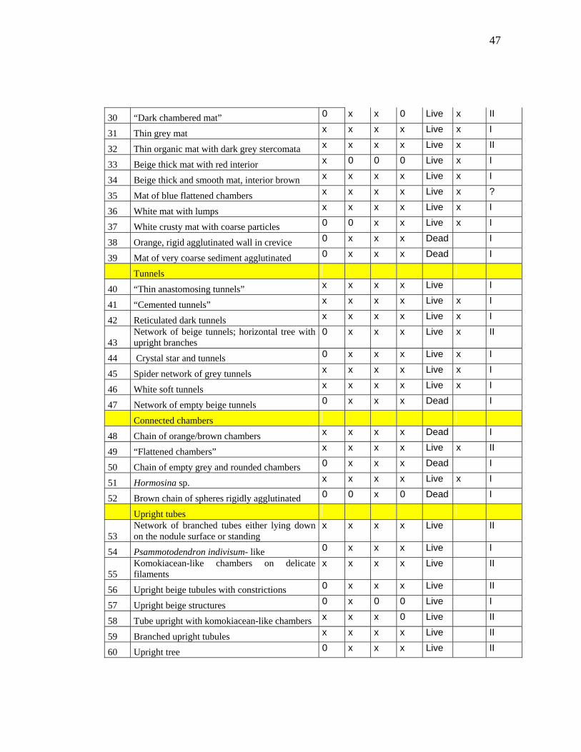
Table 6. List of species colonizing the four facies of the 235 nodules analyzed in this study.

Protozoan species1A2 B2 C2 West2 Live/

Dead3 Percent cover4

Feeding type5

Domes and lumps 1 Pseudowebbinella sp. 0 x x x Live x I

2 Hemispherammina-like, pale regular dome x x x x Live x I

3 Hemispherammina-like, pale granular dome x x x x Live x I

4 Hemisperammina-like, irregular shape x x x x Live x I

5 Tholosina sp. 0 x x 0 Live x I

6 Tholosina-like x x x 0 Live x I

7 Trochammina-like x x x x Live I

8 Placopsilina-like x x x x Live x I

9 Komoki, mud-ball type x x x x Live x II

10 Whitish sparkling dome x 0 0 x Live x I

11 Whitish flattened dome x 0 0 x Live x I

12 White granular patches x x x x Live I

13 Ammocibicides-like x x x x Live x I

14 Fine agglutinated particles beige soft dome x x x x Live x I

15 Brown granular shiny dome 0 x x x Live x II

16 Black granular dome 0 x x x Dead II

17 Black soft dome x x x x Live x II

18 Orange dome x x x x Live x I

Mats

19 Chondrodapis hessleri x x x x Live x II

20 Chondrodapis integra x x x x Live x II

21 Area covered with komokiacean-like chambers linked with fine tubes

x x x x Live x II

22 Grey granular mat x x x x Live x II

23 Very thin muddy patches with komokiacean-like chambers

x x x x Live x II

24 Telammina x x x x Live I

25 Tumidotubus x x x x Live x I

26 Xenophyophorea-like, without agglutinated particles

x x x x Dead II

27 Xenophyophorea-like, fan-shaped agglutinated 0 x x x Dead II

28 “White crust” x x x x Live x I

29 “Beige filamentous mat” 0 x x x Live x ?

47

30 “Dark chambered mat” 0 x x 0 Live x II

31 Thin grey mat x x x x Live x I

32 Thin organic mat with dark grey stercomata x x x x Live x II

33 Beige thick mat with red interior x 0 0 0 Live x I

34 Beige thick and smooth mat, interior brown x x x x Live x I

35 Mat of blue flattened chambers x x x x Live x ?

36 White mat with lumps x x x x Live x I

37 White crusty mat with coarse particles 0 0 x x Live x I

38 Orange, rigid agglutinated wall in crevice 0 x x x Dead I

39 Mat of very coarse sediment agglutinated 0 x x x Dead I

Tunnels 40 “Thin anastomosing tunnels” x x x x Live I

41 “Cemented tunnels” x x x x Live x I

42 Reticulated dark tunnels x x x x Live x I

43 Network of beige tunnels; horizontal tree with upright branches

0 x x x Live x II

44 Crystal star and tunnels 0 x x x Live x I

45 Spider network of grey tunnels x x x x Live x I

46 White soft tunnels x x x x Live x I

47 Network of empty beige tunnels 0 x x x Dead I

Connected chambers 48 Chain of orange/brown chambers x x x x Dead I

49 “Flattened chambers” x x x x Live x II

50 Chain of empty grey and rounded chambers 0 x x x Dead I

51 Hormosina sp. x x x x Live x I

52 Brown chain of spheres rigidly agglutinated 0 0 x 0 Dead I

Upright tubes

53 Network of branched tubes either lying down on the nodule surface or standing

x x x x Live II

54 Psammotodendron indivisum- like 0 x x x Live I

55 Komokiacean-like chambers on delicate filaments

x x x x Live II

56 Upright beige tubules with constrictions 0 x x x Live II

57 Upright beige structures 0 x 0 0 Live I

58 Tube upright with komokiacean-like chambers x x x 0 Live II

59 Branched upright tubules x x x x Live II

60 Upright tree 0 x x x Live II

48

61 Upright filament x x x x Live II

62 Upright filament, branched dichotomously x x x x Live II

63 Upright beige tubule, two origins x 0 0 0 Live II

64 Branching stercomata-filled tube x x x x Live II

65 Anastomosing Rhizammina-like x x x x Live x II

Recumbent tubes 66 Saccorhiza ramosa-like 0 x x x Dead I

67 Tolypammina sp. x x x x Dead I

68 Horizontal organic tube full of stercomata 0 0 x x Live x II

Unattached forms 69 Ammodiscus sp. 0 0 0 x Dead I

70 Orange snail 0 0 0 x Dead I

71 Biloculina sp. 0 x x x Dead I

72 Quinqueloculina-like 0 x x 0 Dead I

73 Thurammina-like 0 0 x 0 Dead I

Metazoan species

Sponges

M1 Taxon 1: Porcupine x x x x Dead S

M2 Taxon 2: Sponge stalk with spikes 0 0 x 0 Dead S

M3 Taxon 3: White rigid stalk 0 0 x 0 Dead S

Scyphozoans

M4 Stephanoscyphus sp. 0 x x x Dead S

M5 Taxon 1: Elongated scyphozoan 0 0 x 0 Dead S

Mollusc

M6 Bentharca asperula 0 x x 0 Live S

Polychaetes

M7 Taxon 1: Spiral 0 x x 0 Dead S

M8 Taxon 2: Smooth tube 0 x x x Dead S

M9 Taxon 3: Tube with spikes 0 0 x 0 Dead S

M10 Taxon 4: Mud tube 0 0 x 0 Dead ?

Bryozoans

M11 Camptoplites sp. 0 x x 0 Dead S

M12 Bugula sp. 0 0 x 0 Dead S

M13 Cyclostomate 0 0 x 0 Dead S

Brachiopods

M14 Pelagodiscus atlanticus 0 0 x 0 Live S

49

M15 Gwynia aff. capsula 0 x x 0 Live S

Ascidian

M16 Cnemidocarpa sp. 0 0 x 0 Live x S

Platyhelminthe, Turbellaria

M17 Fecampia abyssicola 0 0 x 0 Live S 1. Species in quotes have the same name as those described in Mullineaux (1987).2. Presence (x) or absence (0) of the species on nodules. 3. Intact protoplasm was used to identify live specimens, and the “dead” designation was used when only remnant specimens were present on nodule surface. 4. Percent cover identifies species included in the percent cover study. 5. Feeding type I and II for Foraminifera correspond respectively to species without and with stercomata accumulations in their cytoplasm (Gooday et al., 1997), and from morphology and literature descriptions for metazoans (Mullineaux, 1987).

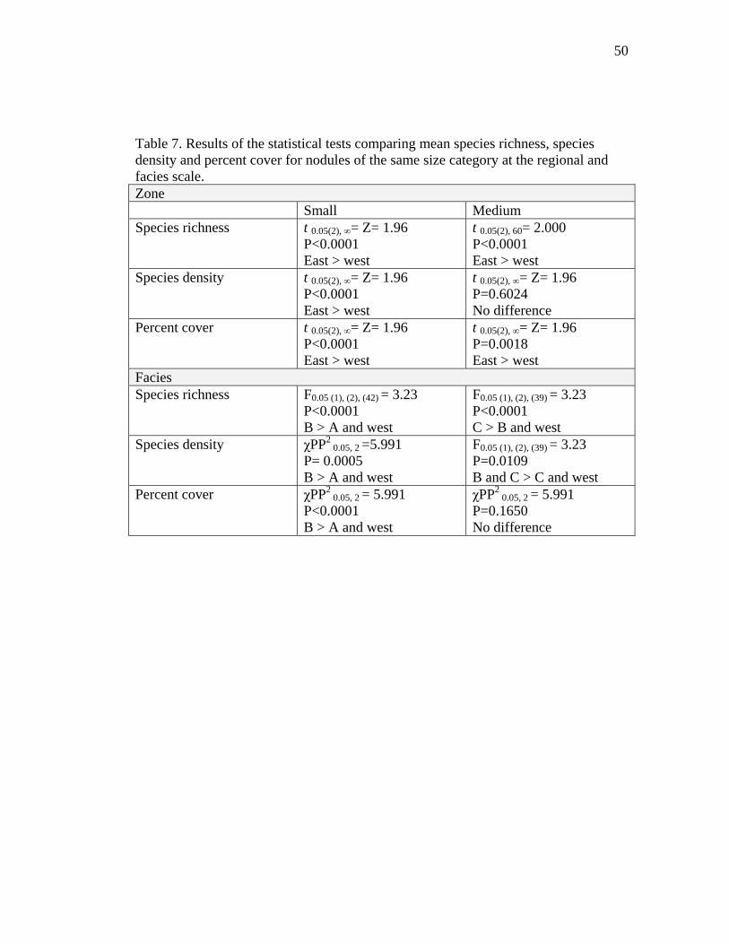
50

Table 7. Results of the statistical tests comparing mean species richness, species density and percent cover for nodules of the same size category at the regional and facies scale. Zone Small Medium Species richness t 0.05(2), ∞= Z= 1.96

P<0.0001 East > west

t 0.05(2), 60= 2.000 P<0.0001 East > west

Species density t 0.05(2), ∞= Z= 1.96 P<0.0001 East > west

t 0.05(2), ∞= Z= 1.96 P=0.6024 No difference

Percent cover t 0.05(2), ∞= Z= 1.96 P<0.0001 East > west

t 0.05(2), ∞= Z= 1.96 P=0.0018 East > west

Facies Species richness F0.05 (1), (2), (42) = 3.23

P<0.0001 B > A and west

F0.05 (1), (2), (39) = 3.23 P<0.0001 C > B and west

Species density χPP2 0.05, 2 =5.991

P= 0.0005 B > A and west

F0.05 (1), (2), (39) = 3.23 P=0.0109 B and C > C and west

Percent cover χPP2 0.05, 2 = 5.991

P<0.0001 B > A and west

χPP2 0.05, 2 = 5.991

P=0.1650 No difference

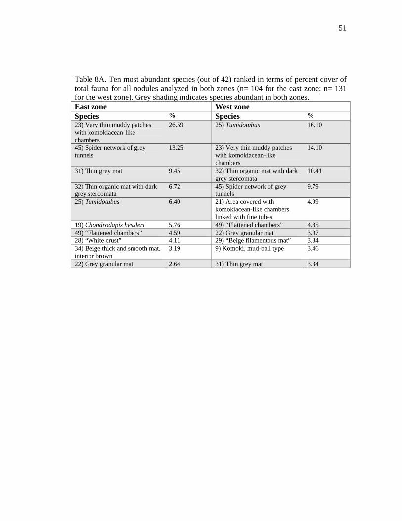
51

Table 8A. Ten most abundant species (out of 42) ranked in terms of percent cover of total fauna for all nodules analyzed in both zones (n= 104 for the east zone; n= 131 for the west zone). Grey shading indicates species abundant in both zones. East zone West zone Species % Species % 23) Very thin muddy patches with komokiacean-like chambers

26.59 25) Tumidotubus 16.10

45) Spider network of grey tunnels

13.25 23) Very thin muddy patches with komokiacean-like chambers

14.10

31) Thin grey mat 9.45 32) Thin organic mat with dark grey stercomata

10.41

32) Thin organic mat with dark grey stercomata

6.72 45) Spider network of grey tunnels

9.79

25) Tumidotubus 6.40 21) Area covered with komokiacean-like chambers linked with fine tubes

4.99

19) Chondrodapis hessleri 5.76 49) “Flattened chambers” 4.85 49) “Flattened chambers” 4.59 22) Grey granular mat 3.97 28) “White crust” 4.11 29) “Beige filamentous mat” 3.84 34) Beige thick and smooth mat, interior brown

3.19 9) Komoki, mud-ball type 3.46

22) Grey granular mat 2.64 31) Thin grey mat 3.34

52

Table 8B. Ten most abundant species (out of 42) ranked in terms of percent cover of total fauna for all nodules analyzed in every facies (A, n= 15; B, n= 50; C, n= 39; west, n= 131). Grey shading indicates species abundant in the four facies. Facies A Facies B Facies C Facies west Species % Species % Species % Species % 23) Very thin muddy patches with komokiacean-like chambers

36.62 23) Very thin muddy patches with komokiacean-like chambers

28.80 23) Very thin muddy patches with komokiacean-like chambers

25.47 25) Tumidotubus 16.10

22) Grey granular mat 7.74 45) Spider network of grey tunnels

17.07 45) Spider network of grey tunnels

12.08 23) Very thin muddy patches with komokiacean-like chambers

14.10

45) Spider network of grey tunnels

7.55 19) Chondrodapis hessleri

7.17 31) Thin grey mat 10.41 32) Thin organic mat with dark grey stercomata

10.41

32) Thin organic mat with dark grey stercomata

7.54 31) Thin grey mat 6.99 25) Tumidotubus 7.39 45) Spider network of grey tunnels

9.79

49) “Flattened chambers”

7.18 32) Thin organic mat with dark grey stercomata

6.44 32) Thin organic mat with dark grey stercomata

6.79 21) Area covered with komokiacean-like chambers linked with fine tubes

4.99

31) Thin grey mat 6.89 22) Grey granular mat 5.86 19) Chondrodapis hessleri

5.36 49) “Flattened chambers”

4.85

25) Tumidotubus 5.74 25) Tumidotubus 3.69 49) “Flattened chambers”

4.91 22) Grey granular mat 3.97

42) Reticulated dark tunnels

4.39 49) “Flattened chambers”

3.42 28) “White crust” 4.82 29) “Beige filamentous mat”

3.84

34) Beige thick and smooth mat, interior brown

3.62 34) Beige thick and smooth mat, interior brown

3.25 34) Beige thick and smooth mat, interior brown

3.15 9) Komoki, mud-ball type

3.46

19) Chondrodapis hessleri

2.71 28) “White crust” 2.30 46) White soft tunnels 2.90 31) Thin grey mat 3.34

53

Table 9. Results of the concordance tests among 42 nodule faunal species: A) overall test and B) a posteriori tests. To avoid spatial bias, 15 nodules were randomly selected from the four facies; five uncolonized nodules (one on facies B and four on facies west) were excluded from the analysis. Hellinger-transformed abundance data for the remaining 55 nodules were used. P= permutational probability based upon 9999 random permutations. PH= Holm adjusted probability for multiple testing. C) Results based on the identification of associated species by K-means partitioning and Pearson correlation matrix. Only species significantly associated within each group by both methods are presented. (* α= 0.05.) A) Overall test of the W statistic. H0: The 42 species are not concordant with one another. Kendall’s W = 0.09164 Friedman’s chi-square = 207.84010 P= 0.0001 * H0 is rejected. Species are not all independent of one another. B) A posteriori tests. H0: This taxon is not concordant with the other 41. 1) Pseudowebbinella sp. P= 0.8427 PH= 3.6864 2) Hemispherammina-like, pale regular dome P= 0.0003 * PH= 0.0117 * 3) Hemispherammina-like, pale granular dome P= 0.0472 * PH= 1.1064 4) Hemisperammina-like, irregular shape P= 0.0471 * PH= 1.1064 5) Tholosina sp. P= 0.0004 * PH= 0.0152 * 6) Tholosina-like P= 0.0354 * PH= 0.9204 8) Placopsilina-like P= 0.0004 * PH= 0.0152 * 9) Komoki, mud-ball type P= 0.0049 * PH= 0.1568 10) Whitish sparkling dome P= 0.4252 PH= 3.6864 11) Whitish flattened dome P= 0.6639 PH= 3.6864 13) Ammocibicides-like P= 0.0001 * PH= 0.0042 * 14) Fine agglutinated particles beige soft dome P= 0.0400 * PH= 1.0000 15) Brown granular shiny dome P= 0.1287 PH= 2.3166 17) Black soft dome P= 0.1911 PH= 2.8688 18) Orange dome P= 0.1169 PH= 2.2211 19) Chondrodapis hessleri P= 0.0001 * PH= 0.0042 * 20) Chondrodapis integra P= 0.1793 PH= 2.8688 21) Area covered with komokiacean-like chambers linked with fine tubes P= 0.0160 * PH= 0.4480 22) Grey granular mat P= 0.2136 PH= 2.9904 23) Very thin muddy patches with komokiacean-like chambers P= 0.2562 PH= 3.0744 25) Tumidotubus P= 0.0006 * PH= 0.0216 * 28) “White crust” P= 0.0002 * PH= 0.0080 * 29) “Beige filamentous mat” P= 0.0103 * PH= 0.2987 30) “Dark chambered mat” P= 0.2736 PH= 3.0744 31) Thin grey mat P= 0.0533 PH= 1.1193 32) Thin organic mat with dark grey stercomata P= 0.0247 * PH= 0.6669 33) Beige thick mat with red interior P= 0.4096 PH= 3.6864 34) Beige thick and smooth mat, interior brown P= 0.0044 * PH= 0.1452 35) Mat of blue flattened chambers P= 0.2191 PH= 2.9904 36) White mat with lumps P= 0.1554 PH= 2.6418 37) White crusty mat with coarse sediments P= 0.0096 * PH= 0.2880 41) “Cemented tunnels” P= 0.0967 PH= 1.9340 42) Reticulated dark tunnels P= 0.6147 PH= 3.6864 43) Network of beige tunnels; horizontal tree with upright branches P= 0.4681 PH= 3.6864 44) Crystal star and tunnels P= 0.0029 * PH= 0.0986 45) Spider network of grey tunnels P= 0.0461 * PH= 1.1064 46) White soft tunnels P= 0.0006 * PH= 0.0216 *

54

49) “Flattened chambers” P= 0.0065 * PH= 0.2015 51) Hormosina sp. P= 0.6139 PH= 3.6864 65) Anastomosing Rhizammina-like P= 0.4104 PH= 3.6864 68) Horizontal organic tube full of stercomata P= 0.9004 PH= 3.6864 M16) Cnemidocarpa sp. P= 0.3645 PH= 3.6450 C) Identification of associated species. Group 1 - 6) Tholosina-like

- 19) Chondrodapis hessleri Group2 - 2) Hemispherammina-like, pale regular dome

- 5) Tholosina sp. - 8) Placopsilina sp. - 21) Area covered with komokiacean-like chambers linked with fine tubes - 36) White mat with lumps - 65) Anastomosing Rhizammina-like

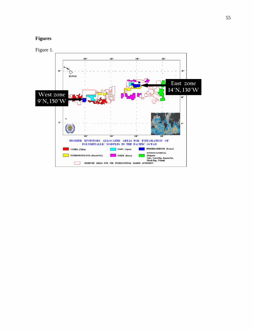
55

Figures Figure 1.

East zone 14°N, 130°W

West zone 9°N, 150°W

56

Figure 2.

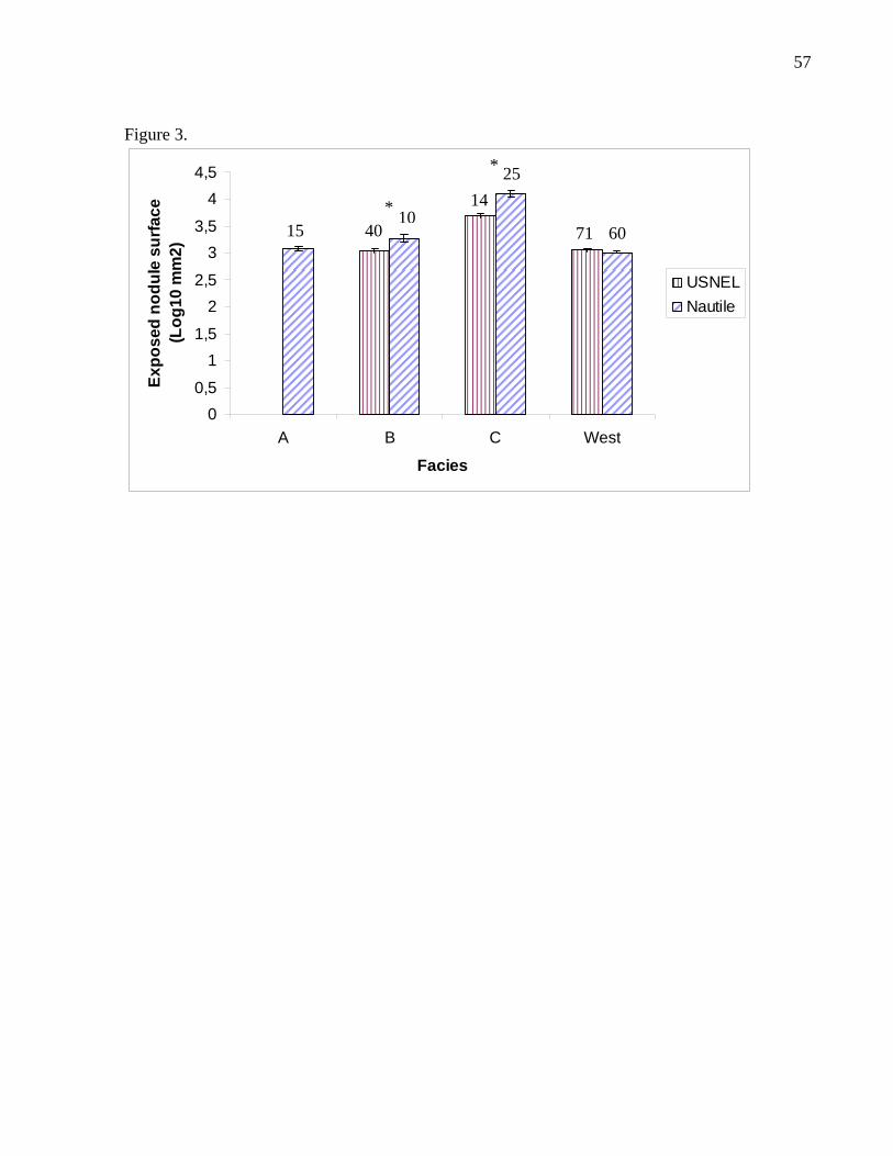
57

Figure 3.

00,5

11,5

22,5

33,5

44,5

Expo

sed

nodu

le s

urfa

ce(L

og10

mm

2)* 5

* 4

05 1 0

1

A B

1

Facies

1

C

2

7

W

6

40

est

USNELNautile

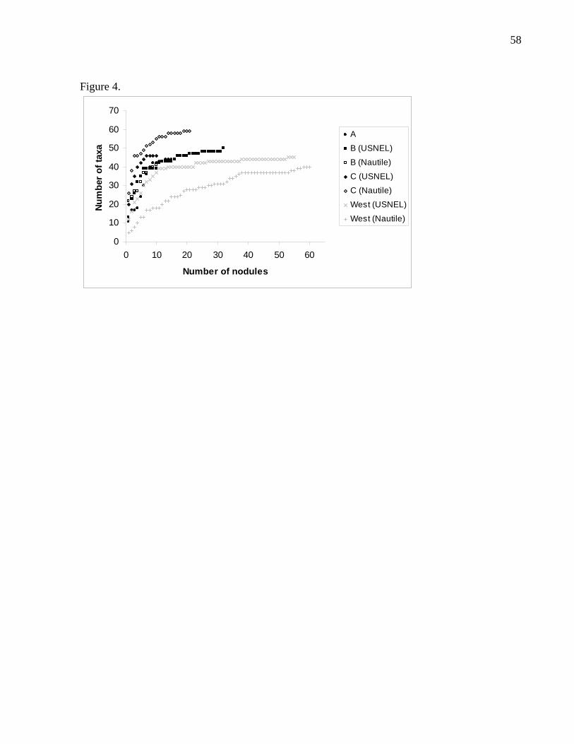
58

Figure 4.

0

10

20

30

40

50

60

70

0 10 20 30 40 50 60

Number of nodules

Num

ber

of ta

xa

A

B (USNEL)

B (Nautile)

C (USNEL)C (Nautile)

West (USNEL)

West (Nautile)

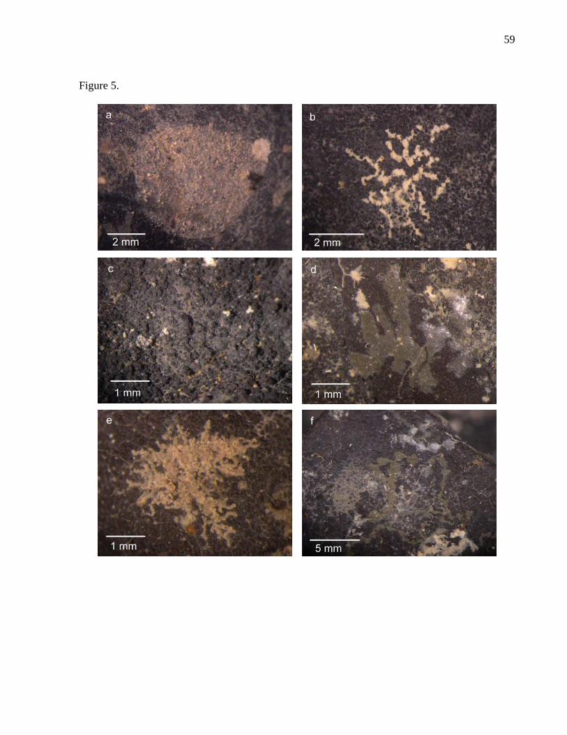
59

Figure 5.

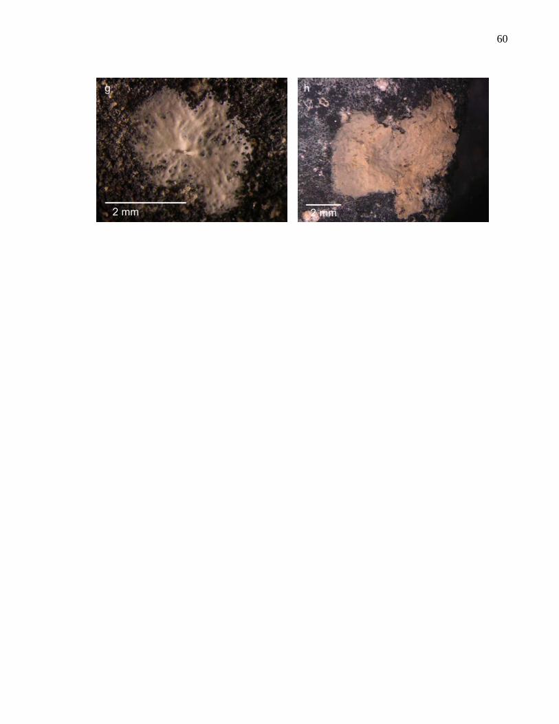
60

61

Figure 6. A) Species richness. B) Species density.

02468

101214161820

East

Num

ber

of ta

xa

0,80,9

1

cm2

*

**

West

Zone

00,10,20,30,40,50,60,7

East West

Zone

Num

ber

of ta

xa p

er

C) Percent cover.

0

1

2

3

4

5

6

East

Perc

ent f

auna

l cov

er

*

**

West

Zone

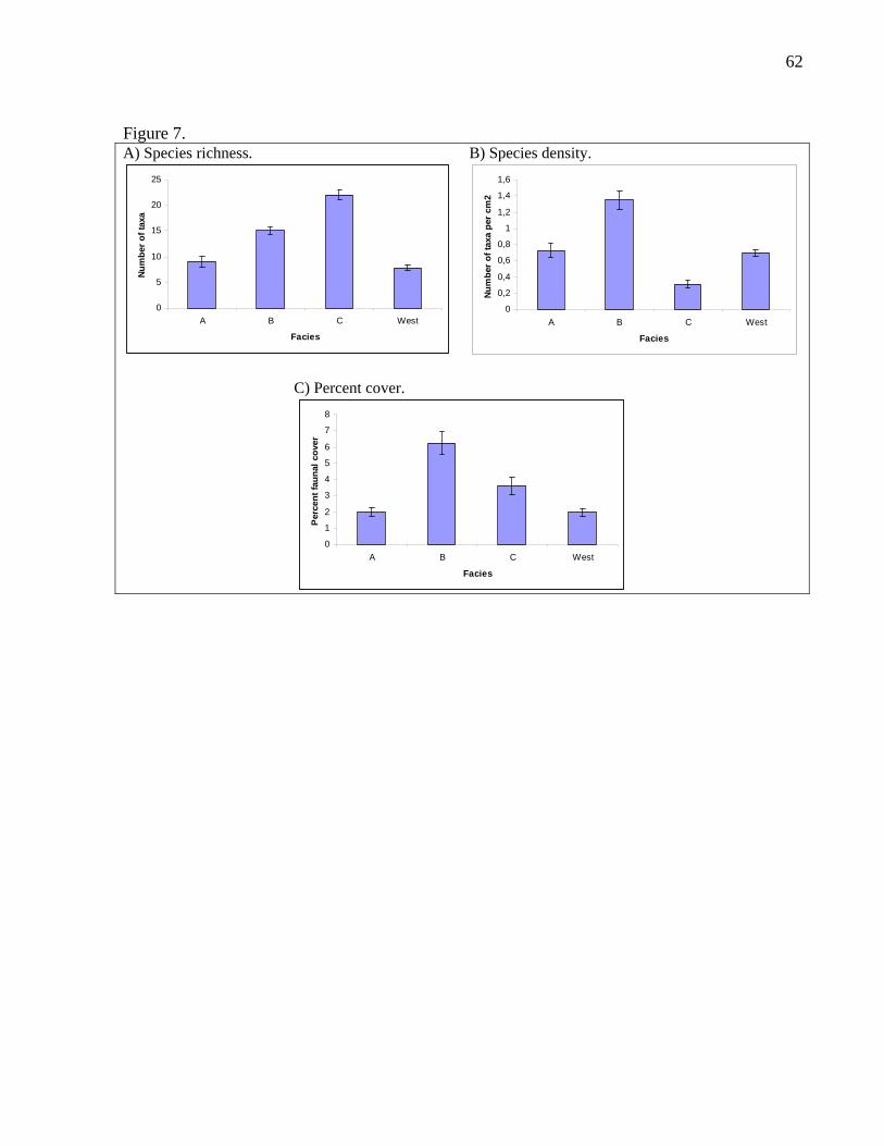
62

Figure 7. A) Species richness. B) Species density.

0

5

10

15

20

25

A B C West

Facies

Num

ber o

f tax

a

0

0,2

0,4

0,6

0,8

1

1,2

1,4

1,6

A B C West

Facies

Num

ber o

f tax

a pe

r cm

2

C) Percent cover.

0

1

2

3

4

5

6

7

8

A B C West

Facies

Per

cent

faun

al c

over

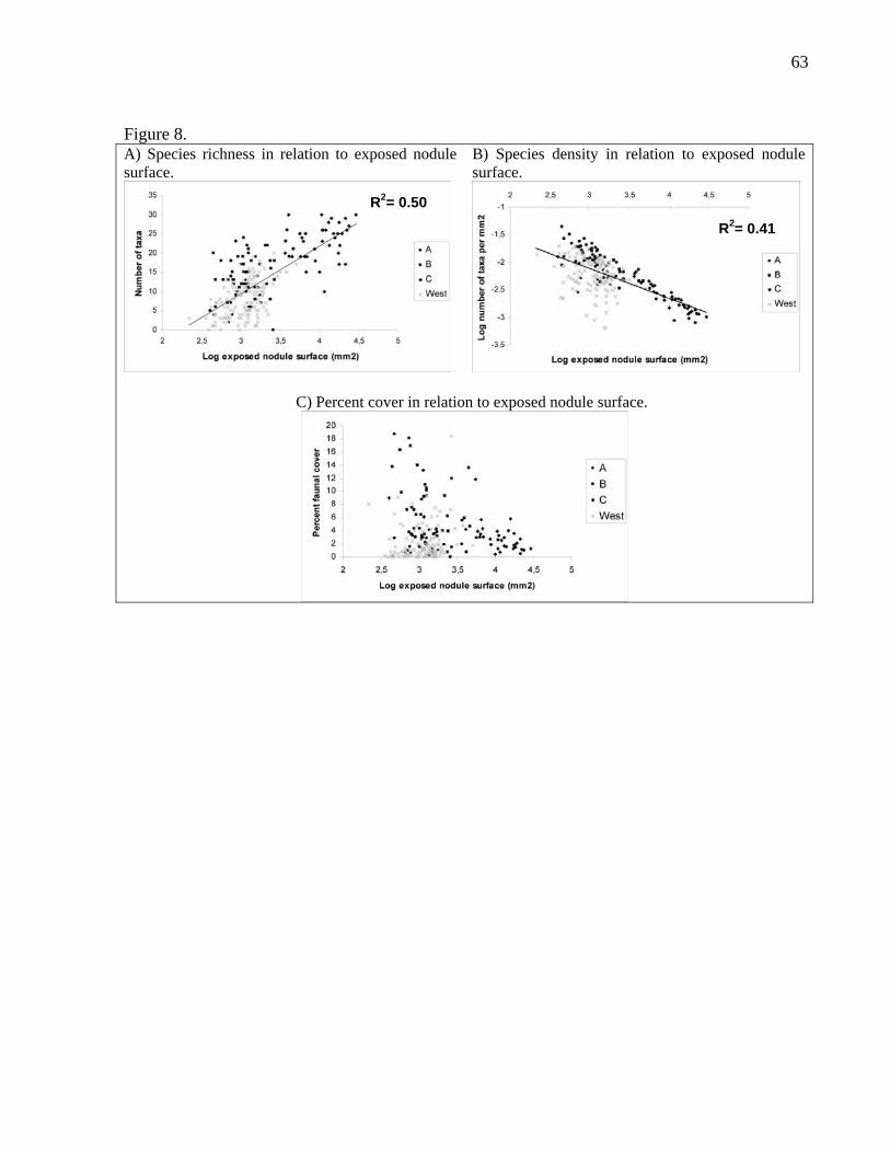
63

Figure 8. A) Species richness in relation to exposed nodule surface.

B) Species density in relation to exposed nodule surface.

C) Percent cover in relation to exposed nodule surface.

R2= 0.50

R2= 0.41

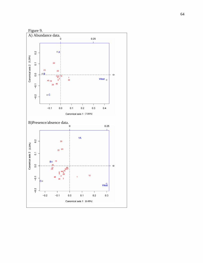
64

Figure 9. A) Abundance data.

B)Presence/absence data.

65

Figure captions Figure 1. Map of the equatorial North Pacific Ocean showing the east and west zones sampled during the present study. Figure 2. Comparison of surface chlorophyll a concentrations for 5˚ boxes around the east and west zones sampled during the present study. Monthly mean surface chlorophyll a derived from SeaWiFS ocean color data. Figure3. Nodule surface area (exposed above sediment line) for the two sampling methods, USNEL box core and the submersible Nautile, for nodules of facies B (50 nodules), C (39 nodules) and west (131 nodules). Numbers of nodules are indicated over bars. Error bars indicate SD. The non-parametric Wilcoxon/Kruskal-Wallis test was used to test differences between the two sampling methods. * α= 0.05. Facies B: Z= 1.96, p= 0,002. Facies C: Z= 1.96, p= 0,03. Facies west: Z= 1.96, p= 0,32. Facies C grouped alone and then, facies A, B and west grouped together according to the Tukey test when nodules of the same facies collected using both sampling methods were pooled together (χPP2

0.05, 3 = 7.815, p<0.0001).

Figure 4. Accumulation curves of taxa for the number of nodules in each facies. Nodules were collected using two sampling methods: USNEL box core and the submersible Nautile. Figure 5. Some of the most common species living on nodule surfaces. a) Very thin muddy patches with komokiacean-like chambers; b) Tumidotubus sp.; c) Thin grey mat; d) Thin organic mat with dark grey stercomata; e) Chondrodapis hessleri; f) “Flattened chambers”; g) “White crust”; h) Beige thick and smooth mat, interior brown Figure 6. Comparison at the regional scale of mean species richness (A), species density (B) and percent cover (C) using all 235 nodules analyzed. Error bars indicate standard error. * α= 0.05, ** α=0.01, ***<0.001. Species richness (t 0.05(2),∞= Z= 1.96, p=0.0000) and percent faunal cover PP (t 0.05(2),∞= Z= 1.96, p<0.0001) were significantly different between the two zones. Only species density (t 0.05(2),∞= Z= 1.96, p= 0.5364) was similar between the two. Figure 7. Comparison at the facies scale of mean species richness (A), species density (B) and percent cover (C) using all 235 nodules analyzed. Error bars indicate standard error of the mean. All tests show significant differences between facies (χPP2

0.05, 3 = 7.815, p<0.0001). Figure 8. Regression of species richness (A), species density (B) and percent cover (C) as a function of exposed nodule surface for the 235 nodules analyzed.

66

Figure 9. Redundancy canonical analysis (RDA) of Hellinger-transformed abundance data (A) (42 species, RPPPPPPPPPPPPPP2 = 0.054, p= 0.0005) and presence/absence data (B) (62 species, R2 = 0.063, p= 0.0001) from 60 randomly-chosen nodules (15 nodules/facies). Nodules without fauna were excluded from the analysis. % of variance explained by each axis indicated between parentheses. Numbers refer to species numbers as detailed in Table 5. Only taxa for which >10% of variance is explained by facies type are shown. 9999 permutations were realized for every test.

67