Embed Size (px)
Citation preview

FEM MODEL OF IMPACTS ON BLADES
Lore Ricquemaque
MSc Thesis Year
Master of Science Thesis
KTH School of Industrial Engineering and Management
Energy Technology EGI-2016-024MSC EKV1134
Division of Heat and Power Technology
SE-100 44 STOCKHOLM

2
Master of Science Thesis, EGI 2016: Nr 024MSC EKV1134
FEM Model of impacts on blades
Lore Ricquemaque
Approved
Examiner
Paul Petrie Repar
Supervisor
Nenad Glodic
Commissioner
Contact person
ABSTRACT
In-service support engineers often have to answer derogations requests regarding impacts on compressor
blades. The stress concentration factor is a physical quantity helping them to take the decisions : it is a measure
of the local increase of the stress due to the impact. Several techniques already exist to derive it like Petersons'
abaci giving it regarding the geometrical parameters of the impact. They are user friendly but conservative in
practice. The most accurate method is zoom-calculation : a Finite Element Model is created to precisely
measure the stress concentration factor. This effective approach is however very time-consuming. In between,
Snecma engineers developed a few years ago a law on the form of abaci derived from a zoom-calculation
results database.
The main purpose of this thesis is to create laws regarding new geometrical parameters and increase the size of
the database following on from the work already carried out. FEM models depending on various parameters
are thus created to derive stress concentration factors. A deep difference from what has been done before
rests on the method : a calculation chain is developed to get results on different sets of impact parameters. It
enables to easily and quickly update the mesh on the models and thus to consider numerous defect
geometries.
The final results of the study are a set of abaci giving the stress concentration factor due to the impact
regarding its geometrical parameters.

3
ACKNOWLEDGEMENTS
I would like to express my gratitude to all the people who guided me during this internship.
I address my deepest thanks to my supervisors M.P. and A.L. for their precious help and advice.
I show my gratitude to D.C., manager of the Rotor Blades and Variable Stator Vane team.
I express special thanks to J.P., C.L., D.E., A.L. and J.M., the specialists who helped me in the decision-making
stage.
I would like to thank S.G., F.G. and V.M. for their support and advice regarding programming : they made me
save precious time.
I am really grateful to Nenad Glodic who supervised my work from KTH.
Lastly, I offer my regards to all of those who supported me in any respect during the completion of the project
and to all the members of the Compressor Blades CEI for their welcome.

4
TABLE OF CONTENTS
Introduction ............................................................................................................................................................ 9
1. Company presentation and context of the study ............................................................................................. 10
1.1. Safran Group .............................................................................................................................................. 10
1.2. Snecma ....................................................................................................................................................... 10
1.2.1 Commercial Engines ............................................................................................................................. 10
1.2.2 Military and space Engines ................................................................................................................... 11
1.3. Compressor blades CEI .............................................................................................................................. 11
1.4. Context ....................................................................................................................................................... 12
1.5. Existing work .............................................................................................................................................. 13
1.5.1. Petersons' Abacus ............................................................................................................................... 13
1.5.2. Zoom-calculation ................................................................................................................................ 14
1.5.3. Snecma experience ............................................................................................................................. 15
2. Objectives of the internship .............................................................................................................................. 16
2.1. General ....................................................................................................................................................... 16
2.2. Deliverables ................................................................................................................................................ 17
2.2.1. Abacus ................................................................................................................................................. 17
2.2.2. Calculation chain ................................................................................................................................. 17
3. Methodology ..................................................................................................................................................... 18
3.1. Starting point : Previous internship............................................................................................................ 18
3.1.1. Existing chain’s functioning ................................................................................................................. 18
3.1.2. Review ................................................................................................................................................. 19
3.2. Gantt chart ................................................................................................................................................. 19
4. Theoretical background .................................................................................................................................... 20
4.1. Rotor blade ................................................................................................................................................. 20
4.2. Defects and impacts ................................................................................................................................... 20
4.2.1. Dent : round bottom ........................................................................................................................... 21
4.2.2. Nick : sharp bottom ............................................................................................................................. 21
4.3. Stress concentration factor and Goodman diagram .................................................................................. 22
4.3.1. Sinusoidal stress .................................................................................................................................. 22
4.3.2. Goodman diagram .............................................................................................................................. 22
4.3.3. Admissible stress concentration factor Kt........................................................................................... 25
4.4. Meshing methods ...................................................................................................................................... 26
4.5. Prestress ..................................................................................................................................................... 28
4.6. Design of experiments ............................................................................................................................... 28
4.6.1. Nominal calculation............................................................................................................................. 28
4.6.2. Tables .................................................................................................................................................. 28
4.6.3. Full Factorial design ............................................................................................................................. 29
4.6.4. Latin-Hypercube design....................................................................................................................... 29
4.7. Groups definition ....................................................................................................................................... 30
5. The chain ........................................................................................................................................................... 31
5.1. Validation and improvement of the existing chain .................................................................................... 31
5.1.1. Programming validation ...................................................................................................................... 31
5.1.2. Models and method validation ........................................................................................................... 32
5.2. Extension .................................................................................................................................................... 36
5.2.1. Trailing edge ........................................................................................................................................ 36
5.2.2. Top of the blade .................................................................................................................................. 36
6. Postprocessing .................................................................................................................................................. 37
6.1 Calculation strategy ..................................................................................................................................... 37

5
6.2. First results and postprocessing strategy for the leading edge ................................................................. 39
6.2.1. Determination of the influential parameters ...................................................................................... 39
6.2. 2. Principal VS Von Mises Kt .................................................................................................................. 39
6.2.3. Comparison to the initial law .............................................................................................................. 41
6.2.4. Postprocessing strategy ...................................................................................................................... 41
6.3. Abacus derivation for the leading edge ..................................................................................................... 43
6.3.1 Practical aspect .................................................................................................................................... 43
6.3.2. Static and modal studies ..................................................................................................................... 44
6.3.3. First derivation .................................................................................................................................... 49
7. Discussion .......................................................................................................................................................... 51
7.1 Results and ongoing actions ........................................................................................................................ 51
7.1.1. Relevance of the points ....................................................................................................................... 51
7.1.2. Abacus derivation ................................................................................................................................ 51
7.1.3 Extensions to other area ...................................................................................................................... 51
7.2 Future work ................................................................................................................................................. 52
Conclusion ............................................................................................................................................................. 52
Annex .................................................................................................................................................................... 53
References ............................................................................................................................................................ 58

6
NOMENCLATURE
Latin symbols
𝐶𝑟𝑖 Criticality
D Distance defining the position of the impact
𝐾 Stiffness matrix
𝐾𝑡 Stress concentration factor
𝐾𝑡𝑎𝑑𝑚 Admissible stress concentration factor
P Principal stress
r Radius of the impact
t Depth of the impact
VM Von Mises stress
𝑋 Nodal displacement vector
Greek symbols
𝛼 Notch angle
𝜎 Stress
Abreviations
CAD Computer Assisted Design
DOF Degree Of Freedom
FEM Finite Element Method
Subscripts
𝑖𝑚𝑝𝑎𝑐𝑡 On the impacted blade
𝑢𝑛𝑑𝑎𝑚 On the undamaged blade
𝑠 Static
𝑑 Dynamic
𝑝 Prestress
reference Relative to the undamaged blade
7
LIST OF FIGURES
Figure 1 : Constraints faced by in service support engineers and their equivalents for the decision support tools .................. 9
Figure 2 : Snecma engines and applications ............................................................................................................................. 11
Figure 3 : Kt determining......................................................................................................................................................... 12
Figure 4 : Is this impact acceptable ?........................................................................................................................................ 12
Figure 5 : Stress concentration factor Ktn for bending of a semi-infinite thin element with a deep hyperbolic notch. .......... 13
Figure 6 : Zoom-calculation method ........................................................................................................................................ 14
Figure 7 : Generalised law giving Kt according to notch parameters, derived from zoom-calculation .................................... 15
Figure 8 : General functioning of the chain. ............................................................................................................................. 18
Figure 9 : Rotor blade parts ...................................................................................................................................................... 20
Figure 10 : a. Defect of type Dent – b. Model of a Dent ........................................................................................................... 21
Figure 11 : a. Defect of type Nick – b. Model of a Nick ............................................................................................................ 21
Figure 12 : Sinusoidal stress ..................................................................................................................................................... 22
Figure 13 : Goodman diagram .................................................................................................................................................. 23
Figure 14 : Adjustment of calculation points on a Goodman diagram method. ...................................................................... 24
Figure 15 : Critical point on a Goodman diagram ..................................................................................................................... 25
Figure 16 : a. Degree 1 or implicit degree 2 elements – b. Explicit degree 2 elements ............................................................ 27
Figure 17 : “Buttonhole effect” ................................................................................................................................................ 27
Figure 18 : Full factorial design for factors X1,X2 and X3. ........................................................................................................ 29
Figure 19 : Latin-Hypercube for 5 experiments in 2D ............................................................................................................... 30
Figure 20 : a. Bottom of the impact (upper part of the chain) – b. Group of elements (lower part of the chain).................... 30
Figure 21 : General convergence study .................................................................................................................................... 32
Figure 22 : a. Results on the impacted blade model on a group that does not include the impact – b. Results on the
reference model at disposal ..................................................................................................................................................... 33
Figure 23 : Maximum stress extracted on the impacted blade ................................................................................................ 34
Figure 24 : Possible places to extract the stresses ................................................................................................................... 34
Figure 25 : Influence of the box size on the Principal stress in the first direction in static and for the modes 1, 5 and 16 ..... 35
Figure 26 : Group of interest for the undamaged blade model ............................................................................................... 35
Figure 27 : CAD model of the blade with an impact on the trailing edge ................................................................................. 36
Figure 28 : CAD model of the blade with an impact on the top (front view). .......................................................................... 36
Figure 29 : CAD model of the blade with an impact on the top (top view). ............................................................................. 37
Figure 30 : Von Mises vs Principal stress concentrations factors. ............................................................................................ 39
Figure 31 : Von Mises stress concentration factors regarding combination 2. ........................................................................ 41
Figure 32 : Example of a law that could be derived. ................................................................................................................ 42
Figure 33 : Von Mises stress concentration factors regarding combination 2 for dents and nicks. ......................................... 43
Figure 34 : Von Mises stress concentration factors regarding combination 2 for the final database. ..................................... 44
Figure 35 : Von Mises stress concentration factors regarding combination 2 for the static case. ........................................... 45
Figure 36 : Von Mises stress concentration factors regarding Von Mises stresses on the undamaged blade for the static
case. ......................................................................................................................................................................................... 45
Figure 37 : Von Mises in the impact regarding Von Mises stresses on the undamaged blade for the static case. ................ 46
Figure 38 : Von Mises stress concentration factors regarding combination 2 for the Mode 2. ............................................... 47
Figure 39 : Von Mises stress concentration factors regarding Von Mises stresses on the undamaged blade for the Mode 2.
................................................................................................................................................................................................. 48
Figure 40 : Goodman diagram for the Mode 2. ........................................................................................................................ 48
Figure 41 : First law derived. .................................................................................................................................................... 49
Figure 42 : Derived law for the flexion modes. ........................................................................................................................ 50

8
LIST OF TABLES
Table 1 : Advantages and drawbacks of the methods to calculate Kt .................................................................. 16
Table 2 : Possible parameters to consider ............................................................................................................ 17
Table 3: Examples of common elements .............................................................................................................. 26
Table 4: Validation strategy .................................................................................................................................. 31
Table 5: Average time to run each step of the chain. ........................................................................................... 38
Table 6: Number of successful experiments lead. ................................................................................................ 38

9
INTRODUCTION
Derogations represent a large amount of the tasks completed by in-service support engineers. The defaults can
be very varied and engineers sometimes have to face new or complex defects whose consequences are difficult
to foresee. They even so have to provide a quick solution to the various problems.
Development of decision support tools are therefore of prime importance in this context. The main challenge is
to create user-friendly tools to answer the time constraint while keeping a sufficient accuracy in the results for
obvious safety reasons in the aerospace industry background. The risk is then to derive very generic and
conservative laws that are useless in practice since no derogation would be acceptable. This problem is
illustrated on figure 1.
Figure 1 : Constraints faced by in service support engineers and their equivalents for the decision support tools.
The purpose of this thesis is a decision support tool which has been developed in order to find the good
balance to fulfill these three constraints.

10
1. COMPANY PRESENTATION AND CONTEXT OF THE STUDY
1.1. SAFRAN GROUP
Safran is a leading international group in high technology industry. In 2014, it employs 69.000 people in 60
countries. Its activities cover all the aerospace market : commercial and military aircrafts, missiles and drones,
space launchers and satellites. The main companies’ activities are described below :
Aerospace propulsion
Snecma : aerospace engine company
Turbomeca : gas turbines for helicopters specialist
Herakles : missile and rocket propulsion specialist
Techspace Aero : equipment and test cells for aerospace engines designer and producer
Aircraft equipment
Messier Bugatti Dowty : landing gears and breaking systems designer and producer
Aircelle : aircraft engine nacelles specialist
Labinal Power Systems : electrical systems for aircraft designer and producer
Hispano-Suiza : power transmission specialist
Defense and security
Sagem : optronics, avionics, electronics and safety-critical software specialist
Morpho : multi-biometric technologies specialist
1.2. SNECMA
Snecma designs, develops and produces alone or in partnership, engines for commercial and military aircraft,
launch vehicles and satellites. In 2015, Snecma had more than 15.000 employees worldwide, working in the 35
plants of the company. It generated 6.5 billion euros annually.
1.2.1 COMMERCIAL ENGINES
Snecma covers a large part of the civil aviation market. The company develops and produces through CFM
International (partnership with General Electric) the CFM56 which powers among other the Airbus A320. The
partners also produce some long-range widebody jets powered by large turbofans such as the CF6, the GE90 or
the GP7200 and they are currently developing the LEAP (Leading Edge Aviation Propulsion) that will equip the
next generation of single-aisle commercial jets. The Silvercrest is under development for business aircrafts. The
Sam 146 is produced with Snecma’s partner NPO Saturn to power the Sukhoi Superjet 100 regional jet.
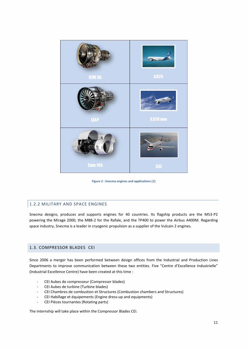
Some of these engines and their associated aircrafts are illustrated figure 2.
11
Figure 2 : Snecma engines and applications [1]
1.2.2 MILITARY AND SPACE ENGINES
Snecma designs, produces and supports engines for 40 countries. Its flagship products are the M53-P2
powering the Mirage 2000, the M88-2 for the Rafale, and the TP400 to power the Airbus A400M. Regarding
space industry, Snecma is a leader in cryogenic propulsion as a supplier of the Vulcain 2 engines.
1.3. COMPRESSOR BLADES CEI
Since 2006 a merger has been performed between design offices from the Industrial and Production Lines
Departments to improve communication between these two entities. Five “Centre d’Excellence Industrielle”
(Industrial Excellence Centre) have been created at this time :
- CEI Aubes de compresseur (Compressor blades) - CEI Aubes de turbine (Turbine blades) - CEI Chambres de combustion et Structures (Combustion chambers and Structures) - CEI Habillage et équipements (Engine dress-up and equipments) - CEI Pièces tournantes (Rotating parts)
The internship will take place within the Compressor Blades CEI.

12
1.4. CONTEXT
Regularly (around every 18000 flight hours), the engine undergoes a shop visit to check its general state. It is
then necessary to determine quickly and easily if an impact on a blade is acceptable or not. A way to take this
decision is to evaluate the stress concentration factor Kt . It is the ratio between the stress on the impacted
blade and the stress on an undamaged one (cf figure 3) [2].
Figure 3 : 𝐊𝐭 determining
This number is then compared to the maximum value of Kt bearable by the blade : Kt adm. The method is
summarized on figure 4.
Figure 4 : Is this impact acceptable ?
13
1.5. EXISTING WORK
Several methods already exist to determine Kt with both advantages and drawbacks.
1.5.1. PETERSONS' ABACUS
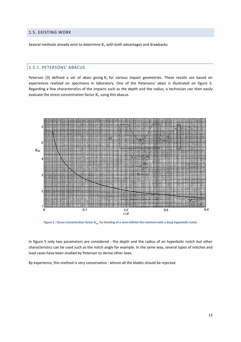
Peterson [3] defined a set of abaci giving Kt for various impact geometries. These results are based on
experiences realized on specimens in laboratory. One of the Petersons' abaci is illustrated on figure 5.
Regarding a few characteristics of the impacts such as the depth and the radius, a technician can then easily
evaluate the stress concentration factor Kt using this abacus.
Figure 5 : Stress concentration factor 𝐊𝐭𝐧 for bending of a semi-infinite thin element with a deep hyperbolic notch.
In figure 5 only two parameters are considered : the depth and the radius of an hyperbolic notch but other
characteristics can be used such as the notch angle for example. In the same way, several types of notches and
load cases have been studied by Peterson to derive other laws.
By experience, this method is very conservative : almost all the blades should be rejected.

14
1.5.2. ZOOM-CALCULATION
Another method is to measure the parameters of the considered impact and to calculate the stress
concentration factor through a very accurate calculation by Finite Element Method (FEM). This method called a
zoom-calculation is illustrated on figure 6.
Figure 6 : Zoom-calculation method
This method is less conservative than the Petersons' one and very accurate. However it is really time-
consuming since the calculations are run in several hours for a specific kind of impact. Besides, it is often quite
difficult for the technician to measure accurately the geometry parameters of the impact (such as the radius or
the angle for example) in practice. A zoom calculation is then meaningless.

15
1.5.3. SNECMA EXPERIENCE
A few years ago several static and dynamic calculations had been run using zoom calculation at Snecma. Among
other things, it led the engineers to extrapolate several laws giving Kt according to different parameters of
impact. One example of the abacus created on that time is given on figure 7. These results have been derived
from calculations on the leading edge.
Figure 7 : Generalised law giving Kt according to notch parameters, derived from zoom-calculation [4]
Each vertical line of points depicts several modes for one set of impacts. The colors correspond to the different
engines considered (several types of blades have also been considered). The generalized law is affine according
to the combination of notch parameters : three different slopes can be used depending on the degree of
conservatism needed.
This law is very accurate since it is based on zoom calculation : it is estimated to be 25% less conservative than
Petersons' abaci. But unlike zoom calculation, it is not valid only for specific cases but for a large range of
parameters (thanks to the extrapolated law). This approach is then a good compromise between the two
previous methods.

16
2. OBJECTIVES OF THE INTERNSHIP
2.1. GENERAL
The main drawbacks and advantages of Peterson abacus, zoom calculation and “Snecma experience” methods
are summarized on table 1.
Zoom calculation Peterson abacus Snecma experience law
Calculation chain
Advantages - Very accurate Results - Little conservative
- Generic - Generic - Little conservative
- Generic - Little conservative - Simulations are run automatically
Drawbacks - Time consuming for each pre processing - Specific - Inconvenient to measure the geometry in practice
- Very conservative - Laborious to run all the calculations “manually”
Table 1 : Advantages and drawbacks of the methods to calculate 𝐊𝐭
Snecma experience principals are thus a method combining both the Peterson abacus spirit and the accuracy of
zoom-calculation : the shape of the abacus is conserved, based on FEM calculation results.
The aim of the internship is to extend the laws already extrapolated by Snecma to other parameters. It could
be done running numerous calculations as the company used to do it but configuring the calculations would be
very arduous and time-consuming.
A solution is to develop a tool running automatically all the calculations. It will be done through a calculation
chain whose main advantage compared to “Snecma experience” method is to run all the simulations
automatically (cf Table 1).
17
2.2. DELIVERABLES
2.2.1. ABACUS
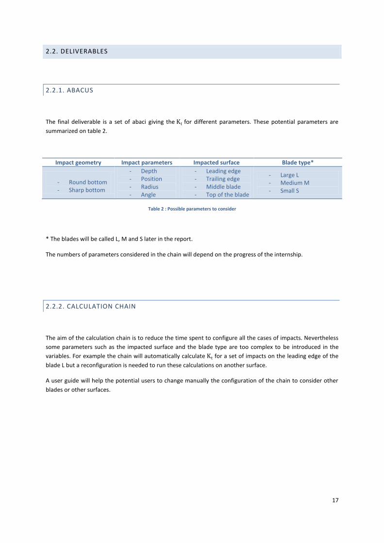
The final deliverable is a set of abaci giving the Kt for different parameters. These potential parameters are
summarized on table 2.
Impact geometry Impact parameters Impacted surface Blade type*
- Round bottom - Sharp bottom
- Depth - Position - Radius - Angle
- Leading edge - Trailing edge - Middle blade - Top of the blade
- Large L - Medium M - Small S
Table 2 : Possible parameters to consider
* The blades will be called L, M and S later in the report.
The numbers of parameters considered in the chain will depend on the progress of the internship.
2.2.2. CALCULATION CHAIN
The aim of the calculation chain is to reduce the time spent to configure all the cases of impacts. Nevertheless
some parameters such as the impacted surface and the blade type are too complex to be introduced in the
variables. For example the chain will automatically calculate Kt for a set of impacts on the leading edge of the
blade L but a reconfiguration is needed to run these calculations on another surface.
A user guide will help the potential users to change manually the configuration of the chain to consider other
blades or other surfaces.
18
3. METHODOLOGY
3.1. STARTING POINT : PREVIOUS INTERNSHIP
A calculation chain has already been set up by a previous intern. Considering a Computer Assisted Design (CAD)
model of a L blade, an impact on the leading edge has been designed on CATIA. The impacted and the
undamaged blade models have then been meshed on Workbench. The stresses are extracted thanks to Samcef
through a calculation on a supercomputer. The previous intern made a functional calculation chain on Optimus.
This software enables to coordinate several calculation tasks and provides experimental methods such as
experimental plans or optimization tools.
3.1.1. EXISTING CHAIN’S FUNCTIONING
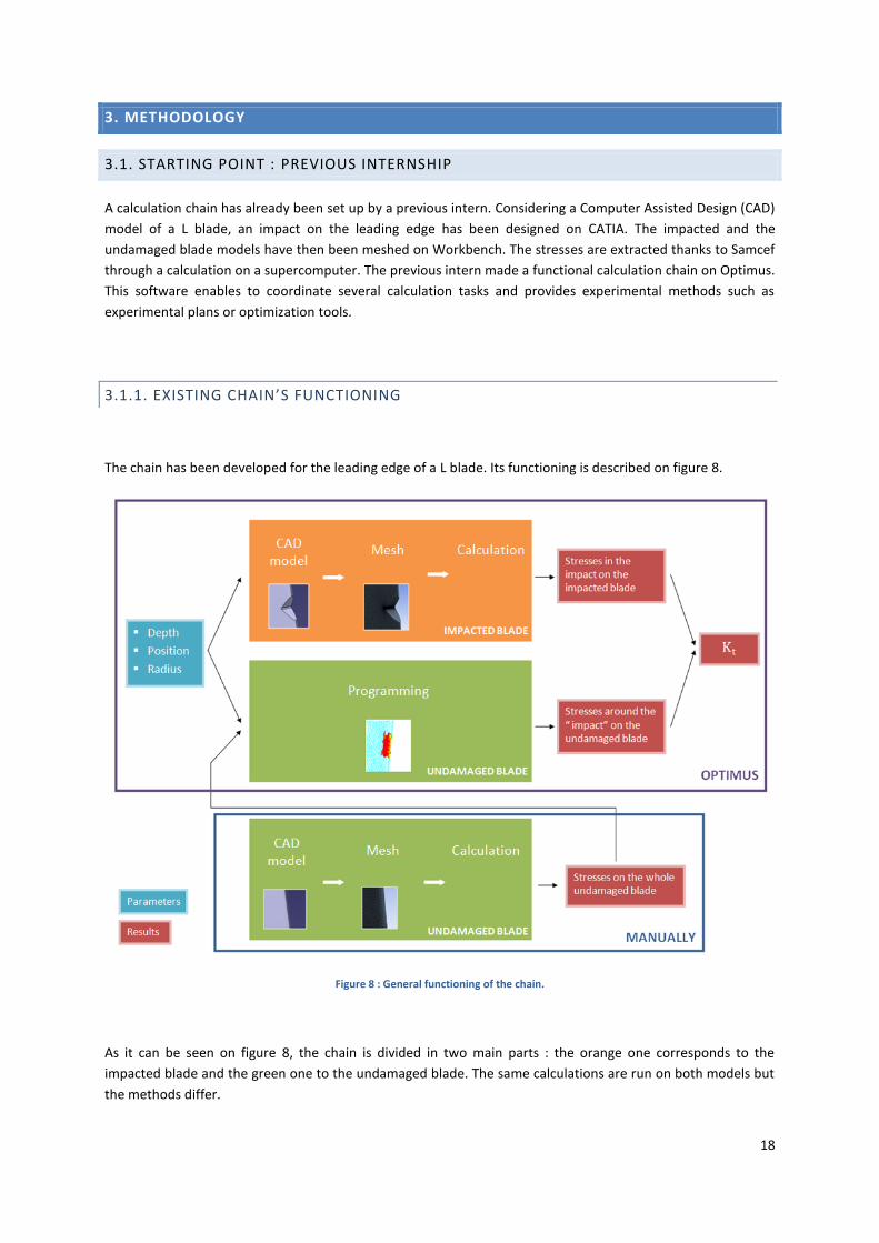
The chain has been developed for the leading edge of a L blade. Its functioning is described on figure 8.
Figure 8 : General functioning of the chain.
As it can be seen on figure 8, the chain is divided in two main parts : the orange one corresponds to the
impacted blade and the green one to the undamaged blade. The same calculations are run on both models but
the methods differ.

19
For example, considering the leading edge of the L blade and a plan of experiments :
- First, the calculations are run “manually” on the undamaged model as described in the lower part of
the figure 8.
- Then, the results files are integrated in the Optimus chain.
- The chain is run for each experience (corresponding to a specific value of depth, position and radius)
automatically.
For each experience, the geometry of the impacted blade is changed so the calculation needs to be rerun. But
it has no influence on the results on the undamaged blade. Therefore, the calculation on this blade is only run
once to save time. The automatic part for the undamaged blade involves extracting the results at the right
position of the undamaged blade (where the impact should be).
3.1.2. REVIEW
The existing chain was working from a programming point of view but it had not been validated : the final and
intermediate results needed to be checked one by one running the different calculations manually.
The CAD model on CATIA and the meshing are specific to the leading edge of the L blade ; the first step after
validation of the chain and post-processing of the first results was to extend the method to other impacted
surfaces and then to other blades.
3.2. GANTT CHART
Numerous softwares and python scripts are used in the existing chain. The first task is thus to get acquainted
with these computer programs. To do so, the methods used to model the impact on the blade and the meshing
are reproduced on a plate. Then this plate is integrated to a new calculation chain on Optimus and the Python
scripts are adapted to the new study case.
This step enables to fully understand the computer programs. It will also make easier the future work involving
the adaptation of the chain to a new blade since it is exactly what I will have to do then.
The second task is to validate the existing chain. Each part of the chain is checked and the results are compared
to references. The first calculations can then be run with the parameters of the existing chain.
Simultaneously, the chain is extended to other surfaces for the future calculations.
The last part of the work will be to run a large plan of experiments and to post process all the results to derive
the abacus.
Several meetings are regularly planned with the supervisors in the company and different specialists of the
subject to check the progress of the internship.
The Gantt chart is presented on Annex 1.

20
4. THEORETICAL BACKGROUND
4.1. ROTOR BLADE
The study is at the moment limited to rotor blades. The different parts composing the blade are described
figure 9.
Figure 9 : Rotor blade parts
The edges, the middle and the top of the blade are the parts concerned by the impacts. The other parts are of
interest in the study regarding the limit conditions.
4.2. DEFECTS AND IMPACTS
Two main type of defects can occur on a blade :
- those whose impact radius cannot be measured : scratches, tears, cracks
- those whose impact radius can be measured
The first ones are considered as cracks and the maximum depth of the defects can be derived through
propagation laws.
The second ones are considered as stress concentration areas whose Kt is calculated as described section 1.4.
Two main geometries are usually used at Snecma to model these defects.

21
4.2.1. DENT : ROUND BOTTOM
This type of impact is smooth, the metal is moved creating light bulges without burs. The part can be deformed.
An example is given figure 10.a.
This defect is usually modeled as described figure 10.b by a depth and a radius.
a. b.
Figure 10 : a. Defect of type Dent – b. Model of a Dent
4.2.2. NICK : SHARP BOTTOM
It is usually caused by an object presenting a sharp corner, leaving a rough surface. The radius is always tiny
due to the plastic deformation of the part. The metal is moved with formation of bulges with burs. There are
usually two straight lines forming an angle. A photography and a model of this defect are given figures 11.a and
11.b.
a. b.
Figure 11 : a. Defect of type Nick – b. Model of a Nick
The use of nicks in the models is more conservative since this type of impact is more aggressive than dents.
22
4.3. STRESS CONCENTRATION FACTOR AND GOODMAN DIAGRAM
4.3.1. SINUSOIDAL STRESS
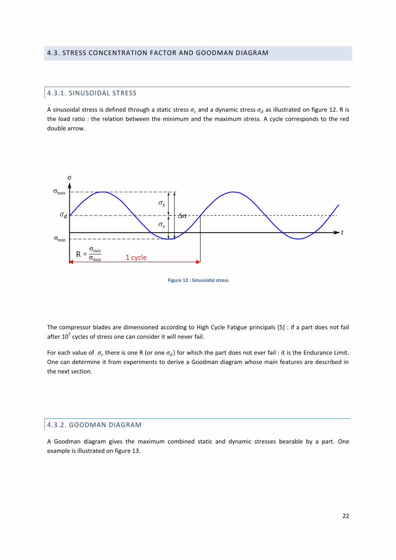
A sinusoidal stress is defined through a static stress 𝜎𝑠 and a dynamic stress 𝜎𝑑 as illustrated on figure 12. R is
the load ratio : the relation between the minimum and the maximum stress. A cycle corresponds to the red
double arrow.
Figure 12 : Sinusoidal stress
The compressor blades are dimensioned according to High Cycle Fatigue principals [5] : if a part does not fail
after 107 cycles of stress one can consider it will never fail.
For each value of 𝜎𝑠 there is one R (or one 𝜎𝑑 ) for which the part does not ever fail : it is the Endurance Limit.
One can determine it from experiments to derive a Goodman diagram whose main features are described in
the next section.
4.3.2. GOODMAN DIAGRAM
A Goodman diagram gives the maximum combined static and dynamic stresses bearable by a part. One
example is illustrated on figure 13.

23
Figure 13 : Goodman diagram
All the points below the black line correspond to specific positions on a part that will not fail. They are derived
from a FEM calculation on a blade. The Goodman diagram can be defined for each mode of excitation.
The first point to reach the endurance limit if all the dynamic stresses are multiplied by a same coefficient is
called the critical point. It is the point C on figure 13. The criticality of any points is defined as below :
𝐶𝑟𝑖(𝑝𝑜𝑖𝑛𝑡) =𝜎𝑑 ,𝑝𝑜𝑖𝑛𝑡
𝜎𝑑 ,𝑔𝑜𝑜𝑑𝑚𝑎𝑛
Equation 1
For the point C :
𝐶𝑟𝑖 𝐶 =𝐶0𝐶
𝐶0𝐶1
Equation 2
In practice, the static stress is derived through a FEM calculation. The dynamic stress is then calculated thanks
to a model with an arbitrary displacement of 1 mm : the maximum absolute displacement is 1 mm in the
calculation results. As a consequence, only the relation between the dynamic stresses at different positions is
correct.

24
The right results are derived trough two steps : Goodman readjustment and engine trials. First, the critical
point is identified and all the dynamic stresses of a mode are multiplied by a same “Goodman” coefficient to
get 𝐶𝑟𝑖 𝑐𝑟𝑖𝑡𝑖𝑐𝑎𝑙 𝑝𝑜𝑖𝑛𝑡 = 1. During the tests, the response to engine excitation is measured for each mode
which enables to readjust the points on the diagram, taking the critical point as a reference.
The method is summarized figure 14.
Figure 14 : Adjustment of calculation points on a Goodman diagram method.
25
4.3.3. ADMISSIBLE STRESS CONCENTRATION FACTOR KT
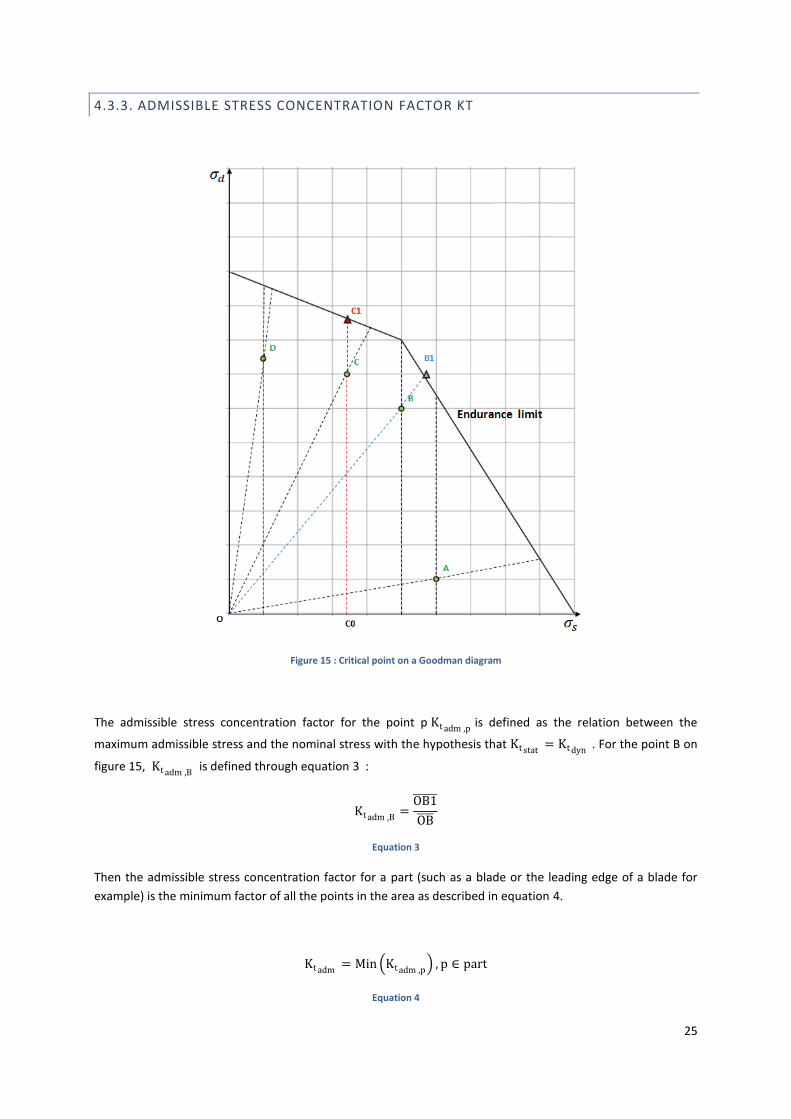
Figure 15 : Critical point on a Goodman diagram
The admissible stress concentration factor for the point p Kt adm ,p is defined as the relation between the
maximum admissible stress and the nominal stress with the hypothesis that Kt stat= Kt dyn
. For the point B on
figure 15, Kt adm ,B is defined through equation 3 :
Kt adm ,B=
OB1
OB
Equation 3
Then the admissible stress concentration factor for a part (such as a blade or the leading edge of a blade for
example) is the minimum factor of all the points in the area as described in equation 4.
Kt adm= Min Kt adm ,p
, p ∈ part
Equation 4

26
Kt adm can then be compared to the stress concentration factor 𝐾𝑡 as described on section 1.4 to determine if
the blade must be rejected or not. Thanks to the abacus created during this internship, it would also be
possible to derive the critical parameters : the maximal depth of an impact at given radius and position for
example.
4.4. MESHING METHODS
The two main characteristics of any element are the degree of freedom (DOF) of the nodes and the degree of
interpolation of the shape functions. To model blades, Snecma usually uses elements of two types : 2D
triangles (or “skin elements”) and 3D tetrahedrons.
Characteristics of common elements are described table 3.
Element Degree of interpolation
Examples (pre/post processing) Examples (solving)
Degree 1 1
Tetra 4
Tetra 4
Implicit degree 2 2
Tetra 4
Tetra 4
Explicit degree 2 2
Tetra 10
Tetra 10
Table 3: Examples of common elements
For tetrahedrons, during pre and post processing, four nodes constitute the element of degree 1 or 2 implicit
(“Tetra 4”) and ten nodes constitute the element of degree 2 explicit (“Tetra 10”).
The degree 2 implicit is created by adding nodes in the middle of the element edges. These nodes are only used
during solving.
27
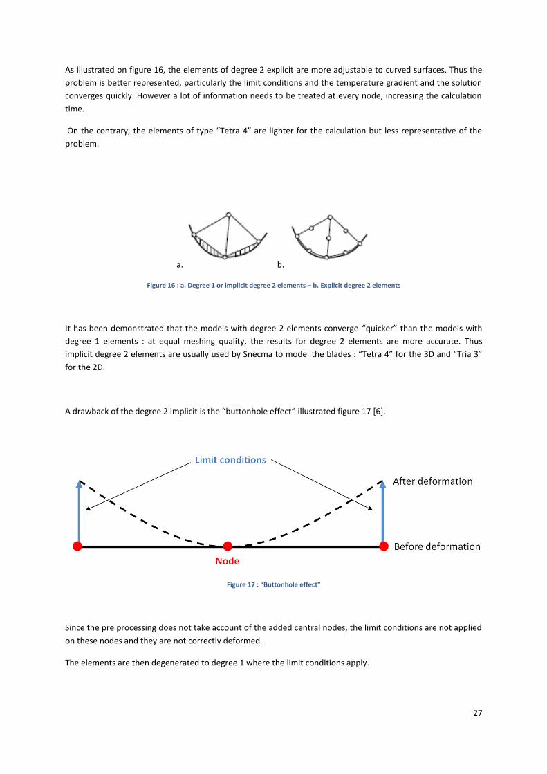
As illustrated on figure 16, the elements of degree 2 explicit are more adjustable to curved surfaces. Thus the
problem is better represented, particularly the limit conditions and the temperature gradient and the solution
converges quickly. However a lot of information needs to be treated at every node, increasing the calculation
time.
On the contrary, the elements of type “Tetra 4” are lighter for the calculation but less representative of the
problem.
a. b.
Figure 16 : a. Degree 1 or implicit degree 2 elements – b. Explicit degree 2 elements
It has been demonstrated that the models with degree 2 elements converge “quicker” than the models with
degree 1 elements : at equal meshing quality, the results for degree 2 elements are more accurate. Thus
implicit degree 2 elements are usually used by Snecma to model the blades : “Tetra 4” for the 3D and “Tria 3”
for the 2D.
A drawback of the degree 2 implicit is the “buttonhole effect” illustrated figure 17 [6].
Figure 17 : “Buttonhole effect”
Since the pre processing does not take account of the added central nodes, the limit conditions are not applied
on these nodes and they are not correctly deformed.
The elements are then degenerated to degree 1 where the limit conditions apply.
28
4.5. PRESTRESS
The blade is subject to the centrifugal force due to its high speed rotation and temperature and pression
gradients. It is thus prestressed. To take into account this phenomenon in the dynamic model, two calculations
are necessary.
The first one is a static calculation described by equation 5 :
𝐹𝑝 = 𝐾𝑝𝑋𝑝
Equation 5
Where 𝐹𝑝 is the prestress force, 𝐾𝑝 the prestress stiffness matrix and 𝑋𝑝 the prestress nodal displacements
vector.
𝐾𝑝 is extracted from this first calculation and used in the second one to adjust the global stiffness matrix K as
described equations 6 and 7 :
𝐹0 + 𝐹𝑝 = 𝐾𝑋
Equation 6
Where 𝑋 is the global nodal displacements vector and𝐾 is defined by :
𝐾 = 𝐾0 + 𝐾𝑝
Equation 7
4.6. DESIGN OF EXPERIMENTS
Optimus enables to use different design of experiments. Those of main interest are described below.
4.6.1. NOMINAL CALCULATION
The chain is run for one specific value of the parameters. It is usually used for validation : a calculation is run
through the chain and “manually” (running all the softwares one after another) at the same time. The results at
each step are then checked.
4.6.2. TABLES
The user defines a set of parameters to be considered by the chain. Like the nominal experiment this method is
used for validation to test the chain on different limit conditions.

29
4.6.3. FULL FACTORIAL DESIGN
The influence of all the parameters needs to be derived individually to create the abacus. A full factorial
evaluates every setting (maximum and minimum) of every factor with every setting of every other parameter.
An example for a three factors full factorial design with three factors is described figure 18.
Figure 18 : Full factorial design for factors X1,X2 and X3. [7]
The effects of multiple factors are investigated simultaneously. And the effects of each parameter are
independent of the remaining parameters.
The obvious drawback of this method is the cost as described on equation 8.
𝑁 = 𝑛𝑖
𝑘
𝑖=1
Equation 8
𝑁 is the number of experiments needed for a design, 𝑘 is the number of factors and 𝑛𝑖 the number of values
for each factor.
The number of experiments increases thus exponentially.
4.6.4. LATIN-HYPERCUBE DESIGN
A nominal calculation for one geometry of impact takes around four hours with a supercomputer. The full
factorial design is then too costly to derive a law. An alternative is the Latin-Hypercube design.
Let 𝑛 be the number of experiments that can be run during a suitable time. Each factor or dimension is divided
in 𝑛 equidistant levels. The experimental points are then selected through a permutation of the levels in all the
dimensions. In this way each level is represented only once in a Latin-Hypercube design. An example in 2D is
given figure 19.
30
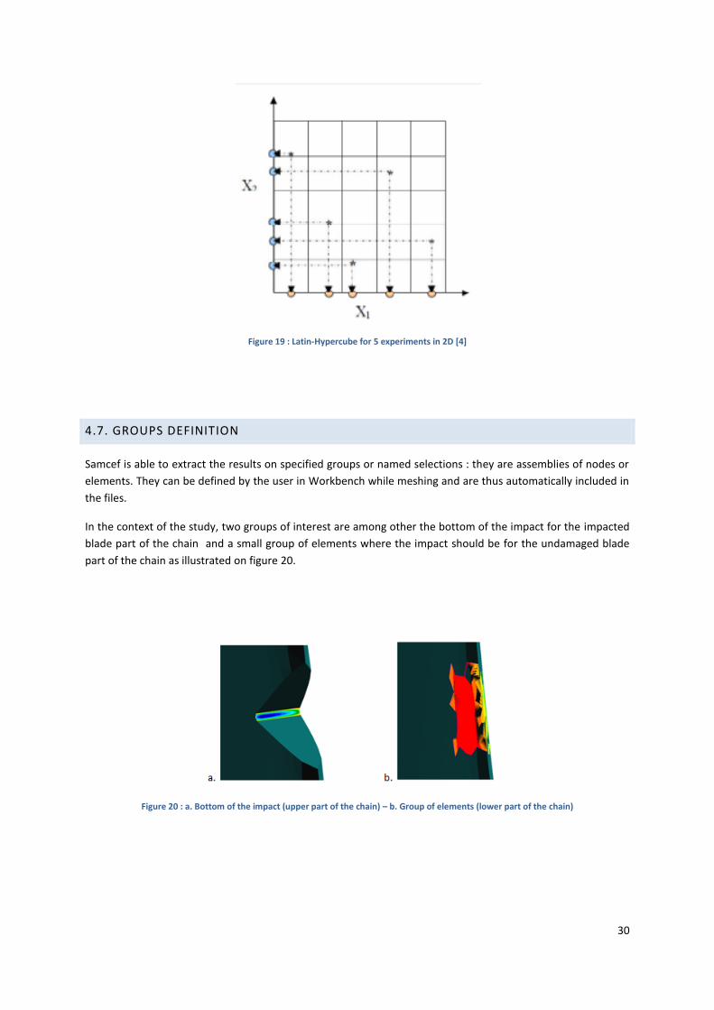
Figure 19 : Latin-Hypercube for 5 experiments in 2D [4]
4.7. GROUPS DEFINITION
Samcef is able to extract the results on specified groups or named selections : they are assemblies of nodes or
elements. They can be defined by the user in Workbench while meshing and are thus automatically included in
the files.
In the context of the study, two groups of interest are among other the bottom of the impact for the impacted
blade part of the chain and a small group of elements where the impact should be for the undamaged blade
part of the chain as illustrated on figure 20.
Figure 20 : a. Bottom of the impact (upper part of the chain) – b. Group of elements (lower part of the chain)
31
5. THE CHAIN
5.1. VALIDATION AND IMPROVEMENT OF THE EXISTING CHAIN
The different steps of the validation and their corresponding sections in the report are summarized below. The
aim is to answer two main questions :
- Is the chain actually doing what it is supposed to do ? In other words, are the results the same if each
step of the chain is run “manually” ? -> 5.1.1. Programming validation
- Are the models relevant ? In other words, if each step of the chain is run “manually”, are the results
correct ? -> 5.1.2. Models and method validation
WB models -> 5.1.2.1.
General method -> 5.1.2.2.
Note : In practice the validation steps have not necessarily been lead in the previous order but they will be
developed this way for clarity reasons.
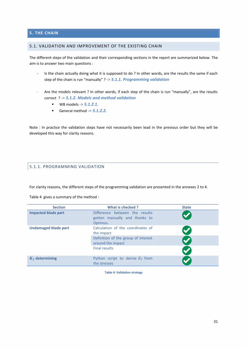
5.1.1. PROGRAMMING VALIDATION
For clarity reasons, the different steps of the programming validation are presented in the annexes 2 to 4.
Table 4 gives a summary of the method :
Section What is checked ? State
Impacted blade part Difference between the results gotten manually and thanks to Optimus.
Undamaged blade part Calculation of the coordinates of the impact Definition of the group of interest around the impact Final results
𝑲𝑻 determining Python script to derive 𝐾𝑇 from
the stresses
Table 4: Validation strategy
32
5.1.2. MODELS AND METHOD VALIDATION
5.1.2.1. WB MODELS
In order to check the Workbench models, two methods have been used.
CONVERGENCE STUDY
This method aims to validate the mesh.
Some results such as the stresses and the deformations are compared to each other for different global mesh
accuracy. The mesh accuracy is improved by decreasing the size of the elements : the more nodes there are,
the more accurate the results are. It is however necessary to refine the elements over all the part to avoid any
“contamination” from the less accurate areas to the more accurate areas.
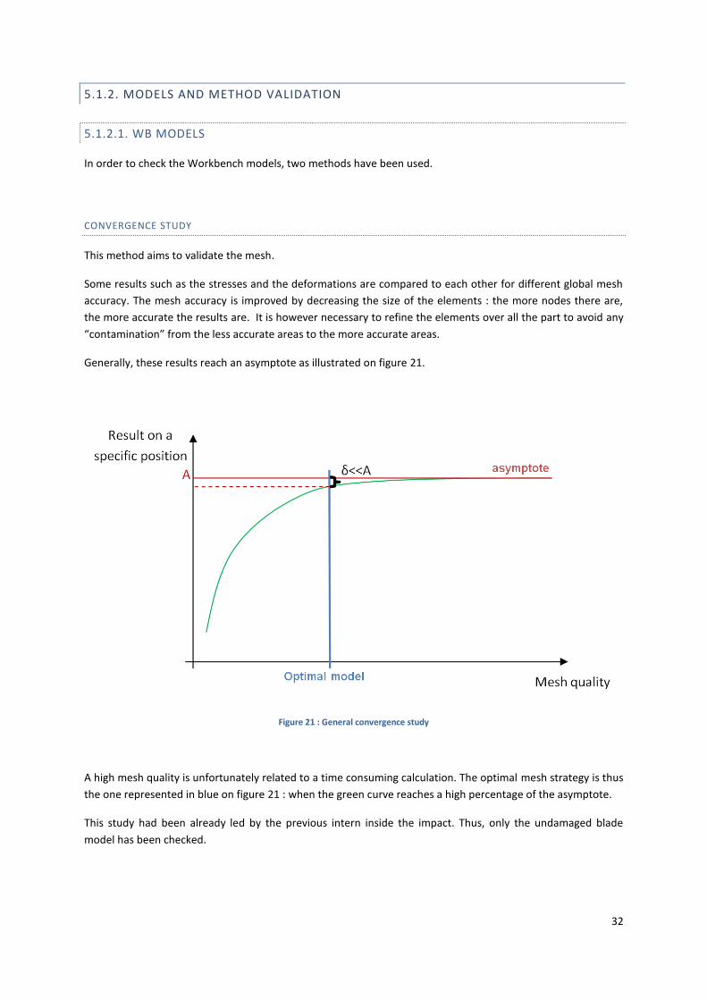
Generally, these results reach an asymptote as illustrated on figure 21.
Figure 21 : General convergence study
A high mesh quality is unfortunately related to a time consuming calculation. The optimal mesh strategy is thus
the one represented in blue on figure 21 : when the green curve reaches a high percentage of the asymptote.
This study had been already led by the previous intern inside the impact. Thus, only the undamaged blade
model has been checked.

33
COMPARISON TO A REFERENCE MODEL
A reference Workbench model of the same blade in the same loading conditions with correct results was at
disposal. It has been used to check three main features of the model
- the initial conditions and CAD model: the materials, the limit conditions, the loading conditions.
- the mesh : number of elements, quality (aspect ratio)
- the results : deformation, stresses
All the characteristics of the first two points have been checked systematically in the tree views of Workbench.
The results have been checked in Patran after a calculation on supercomputer. This method enabled to verify
not only the undamaged blade model but also the impacted blade one thanks to a group including the blade
without the impact as illustrated on figure 22.
a. b.
Figure 22 : a. Results on the impacted blade model on a group that does not include the impact – b. Results on the reference model at
disposal
Despite some differences in the initial conditions, the CAD model and the mesh, the results were very similar
with a maximum error of 3% between the models.
Note : The reference Workbench model could have been used as the undamaged blade model in the chain and
adapted to the impacted blade model. However, some essential features to ensure that it is replayable among
other were missing.

34
5.1.2.2. GENERAL METHOD
ISSUE DEFINITION
According to section 1.4, the stress concentration factor is defined as the ratio between the stress on the
impacted blade and the stress on an undamaged one. In practical, 𝜎𝑖𝑚𝑝𝑎𝑐𝑡 is derived as the maximum stress on
the elements in the bottom of the impact as illustrated on figure 23.
Figure 23 : Maximum stress extracted on the impacted blade
The definition of 𝜎𝑢𝑛𝑑𝑎𝑚 is less obvious. It is supposed to be the stress on the nominal case i.e. the undamaged
case. As a matter of fact, there is a difference of shape between the nominal and the impacted case. Where
should the stress be extracted then ?
1. On the side of the blade at the depth of the bottom of the impact ?
2. On the edge of the blade at the position of the center of the impact ?
3. Inside the blade, at the position of the bottom of the impact (this option has been ruled out since
there is no 2D elements inside the blade) ?
Two hypothesis are illustrated on figure 24.
Figure 24 : Possible places to extract the stresses
𝜎𝑖𝑚𝑝𝑎𝑐𝑡
1
2

35
In practice the group of interest is delimited by a box around the position where the impact should be. A small
box corresponds to the elements of position 2 and a bigger box takes into account all the elements represented
on figure 24 (positions 1 and 2 are thus considered). More details on the box are provided in annex 3.
The box size choice is all the more important that the stresses increase quite fast as we draw away from the
leading edge.
BOX SIZE STUDY
To quantify the influence of the previous issue on 𝐾𝑡 , a study has been lead thanks to the chain. An example is
given on figure 25. The results have been normalized by the values of the stresses over a reference group.
Figure 25 : Influence of the box size on the Principal stress in the first direction in static and for the modes 1, 5 and 16
Some stresses are not influenced by the box size but others such as the principal stress in the first direction are
multiplied by 160 over 1.5 mm of depth.
CONCLUSION
The decision has been made to use the stresses on the edge of the blade around the center of the “impact”
(position 2 on figure 24) as the nominal case. The group used to do so is illustrated on figure 26. It contains all
the elements that share the node.
Figure 26 : Group of interest for the undamaged blade model
0,00
20,00
40,00
60,00
80,00
100,00
120,00
140,00
160,00
0 0,5 1 1,5 2 2,5
No
rmal
ize
d P
1
Box size (mm)
P1 Mode 1
P1 Mode 5
P1 Mode 16
P1 static

36
This method appeared to be quite conservative since it minimizes the box size and thus the stress on the
undamaged blade (as illustrated on figure 25). As this stress is the denominator in the calculation of 𝐾𝑡 , the
stress concentration factor is maximized. Thus there is no risk to under evaluate 𝐾𝑡 .
Another problem of big boxes is the risk to take account of large stresses at a few millimeters of the impact if
the latter is located in a large stress gradient. The derived 𝐾𝑡 would not be linked to the geometry of the impact
but only the position of this one thus.
5.2. EXTENSION
5.2.1. TRAILING EDGE
The same study has been lead on the trailing edge (cf figure 27). The main modifications were on the CAD and
the Workbench models which have been compared to the reference model as previously.
Figure 27 : CAD model of the blade with an impact on the trailing edge
5.2.2. TOP OF THE BLADE
An impact has also been modeled on the top of the blade as illustrated on figure 28.
Figure 28 : CAD model of the blade with an impact on the top (front view).

37
In addition to the CAD and the Workbench models, the definition of the position has also been changed.
Figure 29 : CAD model of the blade with an impact on the top (top view).
One way was to use the geodesic distance between one edge of the blade and the impact (D1 on figure 29) :
the position is accurately defined but it is then complicated to find the node in the center of the impact in the
(X,Y) frame. The position has thus been defined through D2 : the distance between one edge and the impact in
the X-direction. This method enables to easily extract the node of interest but the Latin-Hypercube will not be
defined equidistantly along the centerline of the blade. Besides it will be impossible to derive a direct law based
on the position of the impact but it will be demonstrated below (cf section 6.2.1 ) that such a law cannot be
relevant due to high mode dependency in the dynamic study.
The validation steps were the CAD and Workbench models check in addition to the programming validation :
are the extracted nodes correctly positioned ?
6. POSTPROCESSING
6.1 CALCULATION STRATEGY
As explained on section 4.6.4, latin hypercubes have been used for four parameters : position, depth, radius
and angle. Some tables have also been used to calculate the stress concentration factor for specific sets of
parameters.
Table 5 summarizes the execution time of the main steps of the chain.

38
Table 5 : Average time to run each step of the chain.
For replayable reasons the CAD model cannot bear some impact parameters : the depth has to be superior to
the radius. According to the variation ranges of the parameters, one fourth of the experiments have to be
rejected by Optimus.
Apart from this, the success rate is around 100 %.
The calculations are often run during the weekend. Taking into account the success and rejection rates, that 60
hours are available during the weekend and that one experiment lasts around 5 hours, 16 experiments were
run each week to get 12 results during the calculation steps.
The number of results are summarized on table 6.
Leading Edge Trailing Edge Top
Nicks 11 0 6
Dents 7 0 0
General (4 variables) 44 18 11
Table 6 : Number of successful experiments lead.
For time and clarity reasons, only results on the leading edge are presented in the following sections.
IMPACTED BLADE UNDAMAGED BLADE TOTAL
Step Update the
models
Calculate Extract the stresses
Average time for one
experiment
40 min 4h 12 min 5h

39
6.2. FIRST RESULTS AND POSTPROCESSING STRATEGY FOR THE LEADING EDGE
6.2.1. DETERMINATION OF THE INFLUENTIAL PARAMETERS
The final aim of the internship is to derive a set of abaci giving 𝐾𝑡 regarding the impact parameters : depth,
position, radius and angle or a combination of these ones.
Optimus offers several tools to post process the output data. Among other, correlation values can be derived to
evaluate the influence of each parameter on the results.
The correlation values between the parameters (position, depth, radius and angle and four combinations of
these variables) and the results (stresses and 𝐾𝑡 ) have been studied.
The radius and combinations 1, 2 and 4 are key parameters regarding the stresses on the impacted blade. The
second one is incidentally the combination used in the initial law (cf section 5.1.3).
The sign of the correlation values indicate that any increase of the depth of the impact or any decrease of the
radius or the angle lead to an increase of 𝐾𝑡 .
An attempt has been made to derive a law regarding the position of the impact but without any success since
this parameter is highly dependent on the mode in the dynamic case.
As a consequence, 𝐾𝑡𝑚𝑎𝑥= max𝑖(𝐾𝑡𝑉𝑀 ,𝑖
) is not directly linked to the position of the impact : no law can be
derived.
6.2. 2. PRINCIPAL VS VON MISES KT
Both Principal and Von Mises have been considered in the calculation chain. The importance of each one is
compared on figure 30.
Figure 30 : Von Mises vs Principal stress concentrations factors.
Kt
VM
Kt Principal
Static
Modes
Y=X

40
The stress concentration factor calculated through Principal stresses is then a bit larger than the one derived
through Von Mises stresses for the dynamic case and quite equivalent for the static case.
In the following parts, only Von Mises stresses will be considered since they are easier to interpret and
dimensioning criteria are usually defined through them.

41
6.2.3. COMPARISON TO THE INITIAL LAW
The results have first been compared to this initial law as illustrated on figure 31. The static and dynamic results
are respectively represented in purple and orange. The black lines correspond to the initial law (cf section
5.1.3).
Figure 31 : Von Mises stress concentration factors regarding combination 2.
The mean 𝐾𝑡 appears to be larger than the one derived previously. This is mainly due to the fact that the group
considered to extract the stresses on the undamaged blade was bigger when the initial law had been derived :
it corresponds to a bigger box size in the current study (cf section 5.2.2.2). As a consequence, the nominal
stress used to be more important and the 𝐾𝑡 minimized.
6.2.4. POSTPROCESSING STRATEGY
Since section 6.1.1.1 (Determination of the influential parameters) has highlighted no parameter of greater
interest than combination 2, the laws will all be derived regarding this abscissa.
Two extreme strategies can then be taken on :
- Derive a generic conservative law that includes all the results as illustrated on figure 32 : in practice
the 𝐾𝑡 would be so large even for little impacts that all the blades would be rejected.
- Derive several specific set of abacus : the one used would then depend on the problem studied. As an
example, one can imagine a law for each mode, the abacus used to calculate 𝐾𝑡 being thus chosen
regarding the critical mode. In practice, this method is very unconvenient and time-consuming to use.
The challenge is here to find a law in-between : convenient and not too conservative.

42
Figure 32 : Example of a law that could be derived.
The other point important to highlight here is the relative relevance of the previous results.
Indeed, to get a large database, four parameters have been considered in large scopes of variation but in
practice, the angle and the radius are not measured : a difference is made between nick and dent and the
depth of the defect is measured. Some parameters values that are never encountered can be suppressed.
The 𝐾𝑡 method described part 1.4 Context is generic and convenient but the real dimensioning parameter is
𝜎𝑖𝑚𝑝𝑎𝑐𝑡 . A high 𝐾𝑡 can be due to a large 𝜎𝑖𝑚𝑝𝑎𝑐𝑡 or a small 𝜎𝑢𝑛𝑑𝑎𝑚 . Consequently a high 𝐾𝑡 due to a low 𝜎𝑢𝑛𝑑𝑎𝑚
is not dimensioning and can then be suppressed from the database.
Objective Find the good compromise between a conservative generic law and several inconvenient specific laws
Method Derive some relevant criteria to suppress some results from the database if they are not representative of the reality or if they are not dimensioning for the part
Table 6 : Summary of the postprocessing strategy

43
6.3. ABACUS DERIVATION FOR THE LEADING EDGE
6.3.1 PRACTICAL ASPECT
Since the two principal types of impacts are the dents and the nicks, a study has also been lead on these
specific defects. The results are represented on figure 33.
Figure 33 : Von Mises stress concentration factors regarding combination 2 for dents and nicks.
The results seem to be quite similar to those of the previous part. The 𝐾𝑡 are larger for the nicks as expected
since they are sharper. These defects are more common in practice and more aggressive, the dents are thus
excluded of the study.
Regarding the general results from the previous part, they seem to be quite representative of the reality expect
for the too sharp impacts that do not occur in practice.
Finally the database used to derive the law in the following parts includes the nicks and the general points from
the previous part except the ones that are too sharp (whose radius is inferior to 0.05 mm). This database is
illustrated on figure 34.

44
Figure 34 : Von Mises stress concentration factors regarding combination 2 for the final database.
One hypothesis commonly admitted is 𝐾𝑡 𝑠𝑡𝑎𝑡𝑖𝑐= 𝐾𝑡 𝑑𝑦𝑛
which is not verified on figure 34.
6.3.2. STATIC AND MODAL STUDIES
To understand why some modes give such a high 𝐾𝑡 , it is needed to study them independently.
Note : In this part, several groups of interest have been identified, they are represented with the same
color/shape in the figures 35 to 37 and 38 to 40.
45
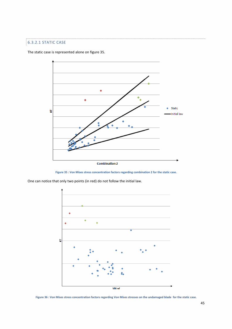
6.3.2.1 STATIC CASE
The static case is represented alone on figure 35.
Figure 35 : Von Mises stress concentration factors regarding combination 2 for the static case.
One can notice that only two points (in red) do not follow the initial law.
Figure 36 : Von Mises stress concentration factors regarding Von Mises stresses on the undamaged blade for the static case.

46
Figure 36 depicts the stress concentration factor regarding the reference stress (on the undamaged blade).
As expected, the highest 𝐾𝑡 (red and green points) correspond to low reference stresses.
Regarding the values of the stresses in the impact and on the undamaged blade that gave such a large Kt on
figure 37, the conclusion is that the stress in the impact for the red points is small compared to the maximum
stress on the leading edge on the undamaged blade (max(VM ref)).
Figure 37 : Von Mises in the impact regarding Von Mises stresses on the undamaged blade for the static case.
These two red points could then be neglected without any risk. On the opposite, the green points cannot be
neglected due to a relative large stress in the impact.
max(VM ref)

47
6.3.2.2. MODE 2
The same study has been led on each mode. An example is given on figures 39 to 41 for the mode 2 which is
particularly scattered.
Figure 38 : Von Mises stress concentration factors regarding combination 2 for the Mode 2.
On figures 38 and 39, the dynamic stresses have been readjusted with “Goodman” coefficients (cf section
4.3.1).

48
Figure 39 : Von Mises stress concentration factors regarding Von Mises stresses on the undamaged blade for the Mode 2.
On figure 39, the stresses on the impacted blade have been written next to the three points with the maximum
𝐾𝑡 .
Figure 40 : Goodman diagram for the Mode 2.
49
Figure 40 represents the Goodman diagram for the mode 2 for the undamaged blade. The critical point of the
blade has been readjusted on the Endurance Limit (orange square) and the critical point of the leading edge is
represented as the red square. The point cloud represents the stresses on the impacted blade.
Triangles
The triangles are the points that would lead to the rejection of the part according to diagram 40. Thus they
cannot be neglected. The yellow triangles are those that give the largest 𝐾𝑡 . One can notice on figure 39 that
the stresses of these points on the impacted blade are largely superior to the maximum stress on the leading
edge of the undamaged blade.
Circles
The red circles below the red line which is parallel to the Endurance Limit line and pass by the critical point of
the leading edge can be neglected. Indeed, they do not increase the criticality of the leading edge.
The circle points are then eliminated from the study for this mode.
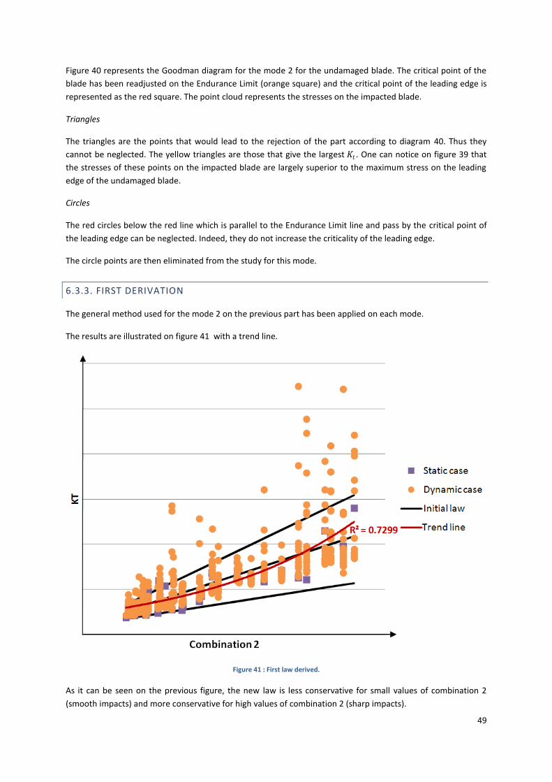
6.3.3. FIRST DERIVATION
The general method used for the mode 2 on the previous part has been applied on each mode.
The results are illustrated on figure 41 with a trend line.
Figure 41 : First law derived.
As it can be seen on the previous figure, the new law is less conservative for small values of combination 2
(smooth impacts) and more conservative for high values of combination 2 (sharp impacts).

50
Since the accuracy of the trend line is not really good, laws depending on the modes have been investigated.
The most relevant is the one for the flexion modes illustrated on figure 43.
Figure 42 : Derived law for the flexion modes.
This law is less conservative than the initial one over all the variation range of the parameters. As an example,
for a same value of 𝐾𝑡 the depth of the impact is increased of 0.5 mm for the new law. The average impact
depth is about 1 mm.
It is quite satisfactory regarding the accuracy (R2 =0.9111) but results only on flexion modes are not sufficient
to study a full blade behavior.

51
7. DISCUSSION
7.1 RESULTS AND ONGOING ACTIONS
The study has not highlighted any parameter more relevant that the ones used previously (combination 2). As a
consequence, the new law is quite similar to the initial one. However it is a bit less conservative and so will
enable the engineers to keep a few more blades than previously. Some improvements can still be considered.
7.1.1. RELEVANCE OF THE POINTS
Only a few points have been eliminated thanks to the method described on part 6.1.2. Some values of the
stress concentration factor are very large and so very detrimental for the law. However they are not always
dangerous since they concern a specific mode which is not necessarily dimensioning for the part. I am currently
trying to neglect more points to get a final less conservative law.
7.1.2. ABACUS DERIVATION
The red curve illustrated on figure 53 is a trend line but other methods can be used to derive a law such as a
piecewise linear function for example. Indeed, the majority of the points for a given set of parameters is small
while a few of them are very high. A linear law ensuring that 80% of the points are under the curve should not
be that conservative thus. I am also currently exploring this option.
7.1.3 EXTENSIONS TO OTHER AREA
A few plans of experiments have been lead on the trailing edge and on the top of the blade. The results are
quite similar to the ones on the leading edge. If a sufficient amount of the points follow the behavior of the law
derived previously, this one will be extend to these areas.

52
7.2 FUTURE WORK
The laws derived during this internship are a bit too conservative in practice. Further study could be led to
improve them. Besides challenging the relevance of each of the calculation points, one could work on a wider
frame than the evaluation of 𝐾𝑡 :
- the dynamical stresses used are only readjusted with "Goodman" coefficients and not with the tests (cf figure
15) : with all the readjustments, the Goodman criteria could be less restrictive.
- in the calculation of 𝐾𝑡𝑎𝑑𝑚, the hypothesis is made that 𝐾𝑡 𝑠𝑡𝑎𝑡𝑖𝑐
= 𝐾𝑡𝑑𝑦𝑛 which is not obvious regarding figure
36 : a different hypothesis could lead to larger values of 𝐾𝑡𝑎𝑑𝑚.
The database elaborated during this internship can be used to derive other kind of laws since more parameters
than the ones used in combination 2 have been used as variables.
Besides the abacus, the other deliverable was a functional calculation chain. Indeed for a given set of
parameters on the leading edge, the trailing edge or the top of the blade, the stress concentration factor can
now easily be calculated : the user only need to run a nominal case.
The chain could be adapted to impacts in the middle bade L and to other kind of blades to lead the same kind
of study.
CONCLUSION
The main challenge of this internship probably lies in the post processing step. Indeed even with accurate
results it has been quite difficult to derive satisfactory laws. It illustrates the problem defined in introduction
regarding the good balance to find between :
- accurate laws for safety reasons
- not too conservative laws for economical reasons
- user-friendly and convenient laws to make quick decisions
This kind of issue is recurrent in all the engineering processes and I found particularly interesting to be able to
consider all these aspects on a concrete case.
Besides the technical skills I acquired using various programs, I had the opportunity to work on a very complete
and diversified subject embedded in the everyday life tasks of the engineers.

53
ANNEX
ANNEX 1 : GANTT CHART
Figure A1 : Gantt chart.

54
ANNEX 2 : PROGRAMMING VALIDATION - IMPACTED BLADE PART
A nominal calculation run on Optimus is compared to a “manual” extraction of the results on the group of
interest (bottom of the impact) in Patran as illustrated on figure A1.
Figure A2 : Von Mises stresses in the impact for the mode i.
Five results are extracted for the static study and twenty modes of the dynamic study :
- The maximum Von Mises stress : 𝑉𝑀
- The maximum Principal stress in the first direction : 𝑃1𝑚𝑎𝑥
- The minimum Principal stress in the first direction : 𝑃1𝑚𝑖𝑛
- The maximum Principal stress in the second direction : 𝑃2𝑚𝑎𝑥
- The minimum Principal stress in the second direction : 𝑃2𝑚𝑖𝑛
The standard deviation is then derived for the static case and the first 20 modes of the dynamic case for Von
Mises and Principals stresses.
The difference between the two methods can be explained by the difference in the mesh : the elements have
been remodeled in the Optimus version since it is done automatically at each new calculation. As a
consequence they are not exactly the same and can be a few less numerous in one or the other methods.
The maximum standard deviation is inferior to 3% which is reasonable.

55
ANNEX 3 : PROGRAMMING VALIDATION - UNDAMAGED BLADE PART
Three critical steps have been checked.
CALCULATION OF THE COORDINATES OF THE IMPACT 𝑥𝐶 ,𝑦𝐶 , 𝑧𝐶 - 𝑥𝑆 ,𝑦𝑆 , 𝑧𝑆 - 𝑥𝐼 ,𝑦𝐼 , 𝑧𝐼
The coordinates of the center of the impact 𝑥𝐶 , 𝑦𝐶 , 𝑧𝐶 in the general frame of work are calculated through a
python script according to the parameter “position”. Then the coordinates 𝑥𝐼 , 𝑦𝐼 , 𝑧𝐼 and 𝑥𝑆 , 𝑦𝑆 , 𝑧𝑠 are derived in
Optimus. Theses points define a box around the impact whose extremities are S and I as described on figure
A3-1.
Figure A3-1 : Box defining a group regarding I and S points.
This box is then used to define the group on the undamaged blade whose stresses will be exctracted.
The coordinates calculated by Optimus are reported on a WB model where the impact is identified as
illustrated on figure A3-2. The nodes 4421, 25310 and 31454 are the closest ones from the edges of the box.
Figure A3-2 : Closest nodes of the coordinates calculated in Optimus in the middle of the blade.

56
DEFINITION OF THE BOX GROUP IN THE CALCULATION FILES
The postprocessing of the result files after the creation of the group of interest on Patran enables to check that
the results are extracted on the right group.
FINAL RESULTS
Similarly to the section 5.1.1.1. the results calculated by Optimus are compared to the results extracted trough
Patran (cf figure A3-4). They are exactly the same since the input files are identical.
Figure A3-3 : Results on the box in Patran

57
ANNEX 4 : PROGRAMMING VALIDATION - 𝐾𝑡 DETERMINING
Note : In the following sections the subscript i can be replaced by “static” or the number of a mode such as
“dyn-15”.
For convenient reasons, all the results will not be conserved to calculate 𝐾𝑡 . A maximum principal stress 𝜎𝑃,𝑖 is
firstly derived for the static study and each modes of the dynamic study according to the equation 9. Then a
Von Mises and a Principal stress concentration factors 𝐾𝑡𝑉𝑀 ,𝑖 and 𝐾𝑡𝑃,𝑖
are calculated for each case (cf
equations 10 and 11).
𝜎𝑃,𝑖 = max(𝑃1𝑚𝑎𝑥 ,𝑖 ,𝑃1𝑚𝑖𝑛 ,𝑖 ,𝑃2𝑚𝑎𝑥 ,𝑖 ,𝑃2𝑚𝑖𝑛 ,𝑖)
Equation 9 : Maximum Principal stress derivation
𝐾𝑡𝑉𝑀 ,𝑖=
(𝜎𝑉𝑀 ,𝑖)𝑖𝑚𝑝𝑎𝑐𝑡𝑒𝑑
(𝜎𝑉𝑀 ,𝑖)𝑢𝑛𝑑𝑎𝑚𝑎𝑔𝑒𝑑
Equation 10 : Von Mises stress concentration factor derivation
𝐾𝑡𝑃,𝑖=
(𝜎𝑃,𝑖)𝑖𝑚𝑝𝑎𝑐𝑡𝑒𝑑
(𝜎𝑃,𝑖)𝑢𝑛𝑑𝑎𝑚𝑎𝑔𝑒𝑑
Equation 11 : Principal stress concentration factor derivation
The number of variables at each step is summarized on figure A4.
Figure A4 : Number of variables available.

58
REFERENCES
[1] Snecma, Commercial Presentation
[2] Theory of Notch Stresses: Principles for Exact Stress Calculation, Heinz Neuber,1945
[3] Peterson’s STRESS CONCENTRATION FACTORS third Edition, edition WILEY by Walter D. & Deborah E. PILKEY
[4] Snecma, Kt_FEM
[5] Fatigue and Durability of Structural Materials, S.S. Manson, G.R. Halford
[6] Modélisation des éléments finis, Jean-Charles Craveur
[7] Optimus users manual


![BLADES [PPT]](https://img.dokumen.tips/doc/110x75/55cf9bc6550346d033a75508/blades-ppt.jpg)