FEM Interface Models for Delamination Analysis

INTERNATIONAL JOURNAL FOR NUMERICAL METHODS IN ENGINEERINGInt. J. Numer. Meth. Engng 2001; 50:1701–1736

Finite element interface models for the delaminationanalysis of laminated composites: mechanical and

computational issues

G. Alfano and M. A. Cris�eld∗;†;‡

Department of Aeronautics; Imperial College of Science; Technology and Medicine; London SW7 2AZ; U.K.

SUMMARY

The �nite element analysis of delamination in laminated composites is addressed using interface elements andan interface damage law. The principles of linear elastic fracture mechanics are indirectly used by equating,in the case of single-mode delamination, the area underneath the traction=relative displacement curve to thecritical energy release rate of the mode under examination. For mixed-mode delamination an interaction modelis used which can ful�l various fracture criteria proposed in the literature. It is then shown that the modelcan be recast in the framework of a more general damage mechanics theory. Numerical results are presentedfor the analyses of a double cantilever beam specimen and for a problem involving multiple delaminationfor which comparisons are made with experimental results. Issues related with the numerical solution of thenon-linear problem of the delamination are discussed, such as the in uence of the interface strength on theconvergence properties and the �nal results, the optimal choice of the iterative matrix in the predictor andthe number of integration points in the interface elements. Copyright ? 2001 John Wiley & Sons, Ltd.

KEY WORDS: delamination; interface elements; �nite elements; fracture mechanics

1. INTRODUCTION

Delamination of laminated composite structures has been widely investigated, from both anexperimental and a numerical standpoint, because it can often be a cause of a local failure and,sometimes, of a sudden structural collapse.The procedures usually followed for the numerical simulation of the delamination can be divided

into two groups. The �rst is based on the direct application of fracture mechanics, while the secondformulates the problem within the framework of either damage mechanics or softening plasticity,or a coupling between the two. When other material non-linearities can be neglected, linear elasticfracture mechanics (LEFM) provides methods which have been proved quite e�ective in predicting

∗Correpondence to: M.A. Cris�eld, Department of Aeronautics, Imperial College of Science, Technology and Medicine,Prince Consort Road, London SW7 2AZ, U.K.

†E-mail: m.cris�[email protected]‡FEA Professor

Contract=grant sponsor: EPSRC

Received 1 March 2000Copyright ? 2001 John Wiley & Sons, Ltd. Revised 16 June 2000

1702 G. ALFANO AND M. A. CRISFIELD

the delamination growth of one or more cracks, provided that their initial position is known inadvance. Techniques such as the virtual crack closure (VCC) [1–3], the J -integral [4], the virtualcrack extension [5], the sti�ness derivative [6], are some of the most used procedures. To modelcrack propagation, the assumption is made that the delamination propagates when the associatedenergy release rate is greater than or equal to a critical value, which is indeed a mechanicalparameter of the interface, a well-established criterion �rst introduced by Gri�th [7].For two-dimensional problems the implementation of these methods is sometimes straightforward

because the crack front propagates in one dimension. However, for three-dimensional problems,the computational burden increases signi�cantly. Furthermore, they cannot be used to predict theinitiation of the delamination and, therefore, they are restricted to problems in which the initialposition of the crack, or ow, is known. Even for 2-D applications, problems arise when morethan one crack propagate simultaneously [8]. For these reasons, a great e�ort has been made todevelop strategies in which the mechanical behaviour of the interface is modelled on the basis ofdamage mechanics and=or softening plasticity combined with an indirect introduction of fracturemechanics [9–22]. These procedures, which may be considered to stem from the work of Hilleborg[9], include the ‘cohesive zone model’ [10; 11]. In relation to the simulation of delamination, themethod has often been applied in conjunction with interface elements [12–22].In this paper, the damage law for the interface elements introduced in References [20–22] for

general mixed-mode delamination is considered and a modi�cation is proposed in order to ensurethat complete delamination occurs simultaneously for all modes, an issue speci�cally consideredalso in References [13; 18]. The interface traction relationship is based on a simple bilinear one-dimensional law which is indirectly related to LEFM in that the area of the triangle delimited bythe traction=relative displacement curve is equated to the critical energy release rate. A high initialpenalty sti�ness is assumed to ensure a reasonable pre-crack behaviour.Special attention must be paid to the choice of the threshold values of the traction components,

toi. It is important for a good prediction of the initiation of the delamination and, in this respect,it should ful�l a failure criterion depending on the material of the interface. Second, it leads todi�erences between the results obtained by a direct use of LEFM and the results of the interfacemodel. Third, it has a strong in uence on the computational e�ciency of the �nite element simu-lation, in that the higher it is, the more re�ned the mesh is required around the delamination front.The last two aspects are discussed in the paper.It will be shown that the proposed interface model can be derived on the basis of a damage

mechanics theory which is similar to the approach adopted for other interface models proposedin the literature [13; 14; 18; 19]. Indeed, the model can be viewed as a regularization of a non-smooth formulation. For a single-mode delamination, the non-smooth model results in an elasticrelationship between the relative displacement and the traction at the interface as long as thespeci�c elastic energy stored is lower than the critical energy release rate Gc, and in a suddenloss of adhesion when = Gc. For mixed-mode delamination, an interaction criterion is adoptedwhich is often used in practical applications [13; 23; 24]. In accordance with this, full delaminationoccurs, and the crack propagates, as soon as an equation is satis�ed which involves the ratiosbetween the dissipated energy for each mode and the critical energy release rate characteristicof the mode itself. Such a criterion has then the advantage that the material parameters involvedcan be experimentally measured by a series of simple single-mode delamination tests. In the non-smooth model, the speci�c energy is then dissipated istantaneously and, generally, at one singlepoint of the interface. Therefore, when the penalty sti�ness in the pre-crack behaviour tends toin�nity, the model reproduces the results of LEFM.

Copyright ? 2001 John Wiley & Sons, Ltd. Int. J. Numer. Meth. Engng 2001; 50:1701–1736

FINITE ELEMENT INTERFACE MODELS 1703

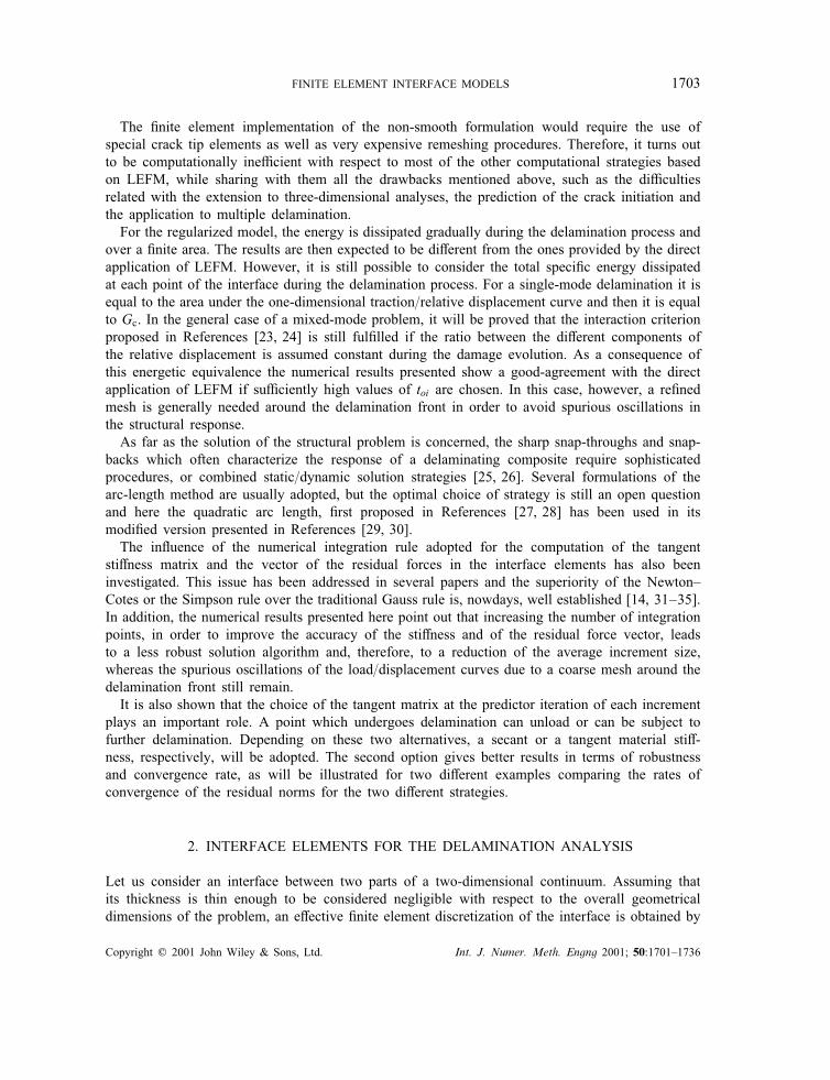
The �nite element implementation of the non-smooth formulation would require the use ofspecial crack tip elements as well as very expensive remeshing procedures. Therefore, it turns outto be computationally ine�cient with respect to most of the other computational strategies basedon LEFM, while sharing with them all the drawbacks mentioned above, such as the di�cultiesrelated with the extension to three-dimensional analyses, the prediction of the crack initiation andthe application to multiple delamination.For the regularized model, the energy is dissipated gradually during the delamination process and

over a �nite area. The results are then expected to be di�erent from the ones provided by the directapplication of LEFM. However, it is still possible to consider the total speci�c energy dissipatedat each point of the interface during the delamination process. For a single-mode delamination it isequal to the area under the one-dimensional traction=relative displacement curve and then it is equalto Gc. In the general case of a mixed-mode problem, it will be proved that the interaction criterionproposed in References [23; 24] is still ful�lled if the ratio between the di�erent components ofthe relative displacement is assumed constant during the damage evolution. As a consequence ofthis energetic equivalence the numerical results presented show a good-agreement with the directapplication of LEFM if su�ciently high values of toi are chosen. In this case, however, a re�nedmesh is generally needed around the delamination front in order to avoid spurious oscillations inthe structural response.As far as the solution of the structural problem is concerned, the sharp snap-throughs and snap-

backs which often characterize the response of a delaminating composite require sophisticatedprocedures, or combined static=dynamic solution strategies [25; 26]. Several formulations of thearc-length method are usually adopted, but the optimal choice of strategy is still an open questionand here the quadratic arc length, �rst proposed in References [27; 28] has been used in itsmodi�ed version presented in References [29; 30].The in uence of the numerical integration rule adopted for the computation of the tangent

sti�ness matrix and the vector of the residual forces in the interface elements has also beeninvestigated. This issue has been addressed in several papers and the superiority of the Newton–Cotes or the Simpson rule over the traditional Gauss rule is, nowdays, well established [14; 31–35].In addition, the numerical results presented here point out that increasing the number of integrationpoints, in order to improve the accuracy of the sti�ness and of the residual force vector, leadsto a less robust solution algorithm and, therefore, to a reduction of the average increment size,whereas the spurious oscillations of the load=displacement curves due to a coarse mesh around thedelamination front still remain.It is also shown that the choice of the tangent matrix at the predictor iteration of each increment

plays an important role. A point which undergoes delamination can unload or can be subject tofurther delamination. Depending on these two alternatives, a secant or a tangent material sti�-ness, respectively, will be adopted. The second option gives better results in terms of robustnessand convergence rate, as will be illustrated for two di�erent examples comparing the rates ofconvergence of the residual norms for the two di�erent strategies.

2. INTERFACE ELEMENTS FOR THE DELAMINATION ANALYSIS

Let us consider an interface between two parts of a two-dimensional continuum. Assuming thatits thickness is thin enough to be considered negligible with respect to the overall geometricaldimensions of the problem, an e�ective �nite element discretization of the interface is obtained by



Figure 1. 4-node interface element. Figure 2. 6-node interface element.

using elements which connect the two parts of the interface whose thickness is taken as exactlyzero (before the deformation of the body occurs) so that, in the 2D case under examination, itresults in a line.We will consider linear 4-node (INT4) and quadratic 6-node (INT6) elements, whose master

elements are shown in Figures 1 and 2, and a geometrically linear theory. In accordance with thezero thickness, the stresses and the strains are in fact interface tractions and relative displacements.In each element we de�ne a local reference system and each relative displacement is the vectorialsum of a traction=compression mode 1 and a sliding mode 2. At the generic point of the interface,it will be denoted by T = (�1; �2) while t = (t1; t2) will indicate the traction.It is convenient to refer the vector p = [p1; : : : ; pn] of the displacement parameters, where n is

4 or 6 for the linear and the quadratic elements, respectively, to the global reference system {ei}and T to the local element one {e′i} so that the matrix B which gives the relationship between Tand p

T(�) = B(�)p (1)

depends upon the rotation of the element and is given by:

B(�) =n∑

i=1Bi(�) with Bi(�) =

[cos � sin �− sin � cos �

] i(�) (2)

where, for i = 1; : : : ; n=2; i(�) is the value at � of the shape function related to node i and i+n=2 = − i.

2.1. The uncoupled model

In this section two uncoupled relationships will be introduced for the single-mode delaminationanalysis. Since in mode 1 the di�erent behaviour in compression and in tension must be takeninto account to avoid penetration, the following notation will be useful:

si[x] ={〈x〉 if i=1|x| if i=2

(3)

where the symbol 〈·〉 denotes the Mc Cauley bracket

〈x〉={x if x¿00 if x60

Furthermore, a pesudo-time parameter is introduced, which is not necessarily the actual time sinceany dynamic e�ects are here neglected. Hence, denoting by [0; T ] the range of interest, �∈ [0; T ]will be the instant under examination.



Figure 3. Uncoupled constitutive relationships.

For the uncoupled model the two bilinear, one-dimensional relationships ti= ti(�i), which aredepicted in Figure 3, are assumed. Their analytical expression is

ti=

Ki�i if (si[�i])max6�oi

or (i=1 and �i¡0)

Ki�i

[1−

((si[�i])max − �oi

(si[�i])max

)(�ci

�ci − �oi

)]if �oi¡(si[�i])max¡�ci

and (i 6=1 or �i¿0)

0 if (si[�i])max¿�ciand (i 6=1 or �i¿0)

(4)

where (si[�i])max denotes the maximum value which has been attained by si[�i]:

(si[�i])max = max06�′6�

si[�i(�′)]

and Ki are penalty sti�ness parameters.By inserting (si[�i])max we take into account the irreversibility of the interface damage, so

that for the relative displacement history depicted in Figure 4(a) we get the traction response ofFigure 4(b). After reaching the value �∗, for decreasing values of � an elastic unloading occurs witha reduced sti�ness which represents the secant from the current point to the origin. Furthermore,after (si[�i])max has exceeded the critical value �ci the traction vanishes as a consequence of thecomplete damage of the interface.When i=1 and �i¡0 relationships (4) ensure no penetration, to within a tolerance which

depends upon the penalty sti�ness parameter K1 adopted.The energy release rate criterion of linear elastic fracture mechanics (LEFM) for the prop-

agation of the delamination in the interface is indirectly used by equating the areas under thetraction=relative displacement curves to the critical energy release rates Gc1 and Gc2. Therefore,



Figure 4. (a) Relative displacement vs time; (b) traction response.

the total energy dissipated during the delamination is correctly computed although at each point itis not released istantaneously as is assumed in LEFM.It is generally assumed that, for laminated composites, Gc1 and Gc2 are characteristic param-

eters of the interface and do not depend on the whole geometry of the composite nor on theapplied loads. They can then be measured by single-mode delamination tests carried out on simplespecimens.The area under the �rst linear branch of the traction=relative displacement curve for the single-

mode i will be denoted with Goi and is given by

Goi= 12Ki�2oi (5)

It represents the speci�c elastic energy stored, at the point of the interface under examination, justat the beginning of the damaging process (Figure 5).When the initiation of the delamination is an issue of concern the values toi should take into

account the actual strength of the interface. In this sense, the tractions at the interfaces must beviewed as interlaminar stresses. Currently we use uncoupled values for to=(to1; to2) although theycould be chosen in accordance with some interactive failure criterion. The choice of to can havea signi�cant in uence on the results of the interface model and on its computational e�ciency. Inparticular, as will be shown by the numerical results presented, the higher are the values of to1and to2, the more re�ned is the mesh that is required around the delamination front. Conversely,excessive small values can result in an unsatisfactory prediction of the delamination.Once the strengths toi are given, the values �ci are obtained by the relationship �ci=2Gci=toi.

The choice of �oi is related to the sti�ness parameters Ki, which could be computed from theelastic moduli of the interface material and its thickness. However, a more convenient approachis to assume Ki as penalty parameters and then choose �oi as small as possible within the rangewhich avoids ill-conditioning.

2.2. The mixed model

In most of the two-dimensional engineering applications, delamination involves both an openingmode 1 and a sliding mode 2. The delamination process involves the dissipation of fracture energyin both modes and the total energy release rate G is the sum of the one G1 associated with theopening mode and the one G2 associated with the sliding mode

G1 =∫ �1

0t1 d�1 G2 =

∫ �2

0t2 d�2 G=G1 + G2 (6)



Figure 5. Speci�c elastic energy at the beginningof delamination.

Figure 6. Tvergaard scaled potential.

Some approaches have been proposed to de�ne a single value Gc of the critical energy releaserate so as to extend, to the mixed-mode analysis, the criterion G=Gc for the propagation of thecrack.In this line is the widely used Tvergaard model [10] (often referred to as a ‘cohesive zone

model’), which assumes that the interface law can be derived by a potential �(�1; �2) given by

�(�1; �2)= �c1

∫ �

0�(�′) d�′ (7)

where �=√(〈�1〉=�c1)2 + (�2=�c2)2 is a damage parameter which ranges from 0 to 1. For the

function �(�) the trapezoidal shape of Figure 6 is sometimes assumed [10; 11] and the total energydissipated at the end of the damage process turns out to be path independent and is given by

G= 12 ��c1(1− �1 + �2) (8)

The formulation has been widely used for the analysis of metals [10; 11]. However, the applica-tion of the model to delamination in composite structures is less straightforward basically because,for di�erent mode ratios, full delamination is achieved with quite di�erent values of G1+G2. Ac-cordingly, the problem arises of de�ning a single value of Gc of the critical energy release ratewhich is strongly dependent on the mode ratio.In particular, with the �xed-mode ratio (FMR) test, a �xed value G1=G2 is de�ned by the

experimental set up and from the experimental results one may obtain Gc appropriate to thisparticular ratio [36]. However, one may not have experimental results for the particular mode ratiounder consideration. In addition, the ratio may be varying.One particular solution, discussed in Reference [21], is to perform a preliminary computation

using LEFM to obtain the mode ratio and then use this value to compute a value of Gc with theaid of an interaction relationship such as the linear relationship given in Reference [23](

G1Gc1

)+(

G2Gc2

)=1 (9)

or the quadratic relationship considered in Reference [24]:(G1Gc1

)2+(

G2Gc2

)2= 1 (10)



or, indeed, the generalized ellipse criterion (GEC) of the form [20–22]

(G1Gc1

)�=2+(

G2Gc2

)�=2= 1 (11)

where � is a material parameter and will generally assume values between 2 and 4. For �=2 and4 the linear criterion (9) and the ellipse criterion (10) are recovered, respectively.Knowing Gc1 and Gc2 from appropriate tests in the separate modes, and the mode ratio G1=G2,

we may then use (9), (10) or (11) to obtain a Gc such that, at propagation:

G1 + G2 =Gc (12)

This was the approach adopted in Reference [21] for using a fracturing criterion based on (12).However, we will here consider an alternative approach which requires no ‘pre-solution’ to

obtain the mode ratio. It is derived from a constitutive model for the mixed-mode delaminationproposed in References [20–22] which ful�ls criterion (11) under certain hypotheses on the historyof the assigned relative displacements and is based on the introduction of the following para-meter � :

� (�)= max06�′6�

(�′) (13)

where

(�′)=[( 〈�1(�′)〉

�o1

)�+( |�2(�′)|

�o2

)�]1=�− 1 (14)

and the explicit dependence on � has been here indicated for the sake of clarity.The constitutive relationship is then given by

t(�)=

{KT(�) if � (�)60

[I −D(�)C(�)]KT(�) if � (�)¿0(15)

where K=diag [Ki], I is the identity matrix, and

D(�)= diag [di(�)] di(�)= max{1;

� (�)1 + � (�)

Fii

}Fii=

�ci�ci − �oi

(16)

The matrix C(�) is de�ned as

C(�)=

[h[�1(�)] 0

0 1

]with h(x)=

{1 if x¿0

0 if x¡0

and ensures that penetration is avoided to within the numerical penalty sti�ness adopted.It is easy to verify that relationships (13)–(16) specialize to Equations (4) for a single-mode

delamination problem. Notice also that, as a consequence of the irreversibility of the damage, � isa monotonic increasing function of �. In the sequel, for simplicity, if the explicit dependence of avalue upon the pseudo-time parameter is omitted, it is understood that the value is to be computedat the current time �.



By di�erentiating relationship (15), and introducing the diagonal matrix A=diag [1=��oi] and the

notation:

T=[〈�1〉|�2|

]Tx =

[〈�1〉x|�2|x

]∀x∈<+

the following expression of the constitutive tangent operator is obtained:

Kt =

K if � 60

(I −DC)K − 1(1 + � )1+�FK(T⊗ T

�−1)A if � = ¿0

(I −DC)K if ¡� ¿0

(17)

with the further condition:

(Kt)ij =0; j=1; 2 if di¿1 (18)

Notice that the case ¡� ¿0 is recovered in the one-dimensional example of Figure 4 when�∗1¡�¡�∗2 and then the term (I − DC)K represents the secant sti�ness characteristic of the un-loading path.

Remark 2.1. The proof that relationships (13)–(16) ful�l criterion (11) has been given in theinternal report [37] under the assumption of a �xed-mode ratio. For completeness it is reported inAppendix D eliminating the unnecessary hypothesis that �o1 = �o2. Later on in the paper the sameresult will be proved in the general framework of damage mechanics.

2.3. A modi�ed constitutive relationship

In accordance with relationships (13)–(16), complete debonding of one point of the interfaceis, in general, reached at two-di�erent times for modes 1 and 2. This is inconsistent with thephysical evidence that complete debonding allows both the opening and the sliding mode to beactivated, simultaneously, with a null value of the resultant traction (unless compression occurs).Some authors add this consistency condition as a further constraint to the evolution equations forthe damage parameters [13; 18]. In the model here presented, this problem can be avoided if theratios �o1=�c1 and �o2=�c2 are equal. Since the parameters �o1 and �o2 are mainly related to thepenalty sti�ness, such an assumption does not give any restrictions and therefore it will be madein the sequel, unless it is di�erently speci�ed. Introducing the following parameter �:

�=1− �o1

�c1= 1− �o2

�c2(19)

the modi�ed constitutive relationship which is here used for the mixed-mode analysis is then asfollows:

t=

{KT if � 6 0

[I − dC]KT if � ¿0(20)

where

d= max{1;1�

(�

1 + �

)}(21)

and the parameter � is given in Equation (13).



Remark 2.2. The mixed-mode formulation here presented has close links with that proposed inReference [13]. The specialization of the formulation is there based on isotropic damage of theinterface and can be recast into the following equations:{

t=KT if � 6 0

t=(1− � )KT if 0¡ ¡ 1

(22)

where � is a damage parameter de�ned as:

� = max�′6�

√∑

i

(�i

�oi

)2�− 1 (23)

The meaning of � is similar to that of � in Equation (14) in that, for a delamination processwith a �xed mode ratio, criterion (11) is ful�lled with �= �=2.The parameter is dependent on the value of Gc for each mode. In fact, in order to ensure

that, for a case of single-mode delamination, the speci�c dissipated energy be equal to Gc, thefollowing relationship must be satis�ed:

GciGoi

=�

� + 2

[( + 1

)(�+2)=�− 1]

(24)

The basic di�erence between the two models seems to lie in the shape of the traction=relativedisplacement curve for a single-mode case. With the model proposed in Reference [13] a non-linear law is used so that the non-smoothness of the relationship is reduced. On the other hand,an advantage of the model here presented is that the values of Gci are directly required as inputparameters.

3. DAMAGE MECHANICS FORMULATION

In this section the interface model presented in Section 2 is recast in a framework typical ofa damage mechanics theory. We �rst consider the one-dimensional model and then mixed-modedelamination will be addressed.

3.1. One-dimensional model

Let us consider one single-mode and rule out the case of a negative value of the relative dis-placement, so as to simplify the notation by eliminating any sign issues, and assume the followingexpression of the free energy potential:

(�; d)= 12 (1− d)K�2 (25)

The di�erentiation of provides the relationship between the couple (�; d) and its work-conjugate couple of variables (t; Y ):

t=d d�=(1− d)K�

Y = − d d�=12K�2

(26)



Remark 3.1. The dual parameters d and Y are internal variables of the model which accountfor the debonding of the interface and the product Y d represents the speci�c energy dissipating inthe damage process at the current time �.In this respect it is worth recalling the well-known mechanical interpretation of d as a measure

of the microvoids which occur in the interface at a micromechanical scale, that is, referring to anin�nitesimal part of the interface, a ratio between the area complementary to the e�ective load-bearing part and the nominal area [38; 39]. Hence, Y is the speci�c elastic energy which wouldbe stored if the interface was undamaged, Yd is the speci�c energy which is actually stored andY d represents the speci�c energy released when the damage grows, for a �xed value of �, whichalso explains the minus sign conventionally adopted in Equation (26)2.

Equations (26) do not fully de�ne the constitutive behaviour of the interface and an evolutionlaw must be assumed. This can be done by de�ning a damage threshold Yc, depending on d, andintroducing the following Khun–Tucker conditions:

Y 6Yc d¿ 0 (Y − Yc) · d=0 (27)

with the further constraint

06d6 1 (28)

The choice of the relationship between Yc and d results in di�erent damage models. A �rstpossibility consists of assuming that no damage occurs as long as Y keeps constantly lower thanthe critical value Gc of the energy release rate and that complete damage is obtained as soon asY attains the value Gc. It can be recovered if the following relationship is assumed between Ycand d:

Yc =Gc if 06d¡1

Yc = �Y if d=1(29)

where

�Y (�)= max�′¡�

Y (�′)=12K�2max (30)

Remark 3.2. Notice that (29) is a multivalued law since, for d=1; Yc can assume in�nitevalues. However, this fact does not have any mechanical implications since, for d=1; d is neces-sarily zero. Then the dissipation Y d is zero, as well, so that the value of Y assumes a pure formalmeaning.

In accordance with Equation (27)2−3, a positive value of d is associated only with a constantvalue of Y =Yc or, equivalently, Y =Gc. The total speci�c energy dissipated is then equal to Gc:∫ +∞

0Y · d dt=Gc (31)

Moreover, since this energy can be thought of as being dissipated instantaneously, the di�erencefrom the application of LEFM is only that the �nite value of the penalty sti�ness allows a non-zeroelastic relative displacement before the damage of the interface occurs.The model proposed in Section 2 can be recovered from this non-smooth formulation if the

value of the tensile strength is such that the softening lines of the curves in Figure 3 degenerate



to vertical lines or, equivalently, if the values �o and �c coincide. In that case, the energy Go

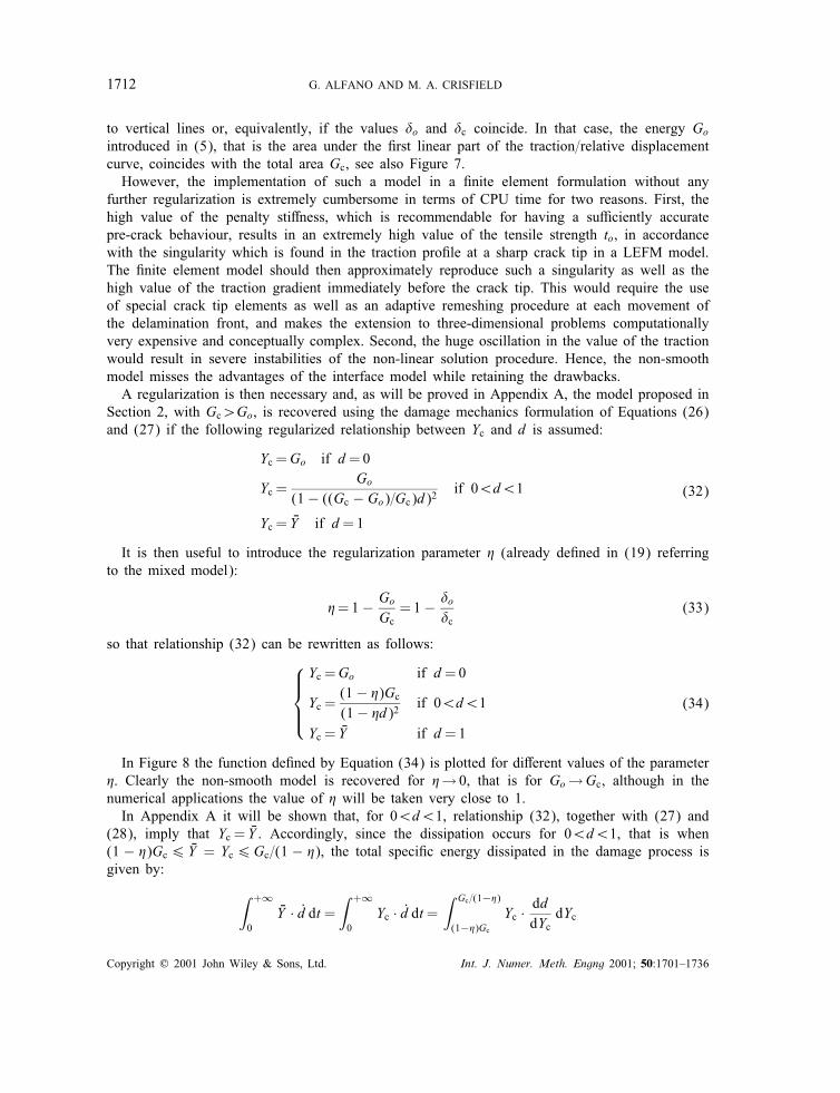
introduced in (5), that is the area under the �rst linear part of the traction=relative displacementcurve, coincides with the total area Gc, see also Figure 7.However, the implementation of such a model in a �nite element formulation without any

further regularization is extremely cumbersome in terms of CPU time for two reasons. First, thehigh value of the penalty sti�ness, which is recommendable for having a su�ciently accuratepre-crack behaviour, results in an extremely high value of the tensile strength to, in accordancewith the singularity which is found in the traction pro�le at a sharp crack tip in a LEFM model.The �nite element model should then approximately reproduce such a singularity as well as thehigh value of the traction gradient immediately before the crack tip. This would require the useof special crack tip elements as well as an adaptive remeshing procedure at each movement ofthe delamination front, and makes the extension to three-dimensional problems computationallyvery expensive and conceptually complex. Second, the huge oscillation in the value of the tractionwould result in severe instabilities of the non-linear solution procedure. Hence, the non-smoothmodel misses the advantages of the interface model while retaining the drawbacks.A regularization is then necessary and, as will be proved in Appendix A, the model proposed in

Section 2, with Gc¿Go, is recovered using the damage mechanics formulation of Equations (26)and (27) if the following regularized relationship between Yc and d is assumed:

Yc =Go if d=0

Yc =Go

(1− ((Gc − Go)=Gc)d)2if 0¡d¡1

Yc = �Y if d=1

(32)

It is then useful to introduce the regularization parameter � (already de�ned in (19) referringto the mixed model):

�=1− Go

Gc= 1− �o

�c(33)

so that relationship (32) can be rewritten as follows:

Yc =Go if d=0

Yc =(1− �)Gc(1− �d)2

if 0¡d¡1

Yc = �Y if d=1

(34)

In Figure 8 the function de�ned by Equation (34) is plotted for di�erent values of the parameter�. Clearly the non-smooth model is recovered for �→ 0, that is for Go →Gc, although in thenumerical applications the value of � will be taken very close to 1.In Appendix A it will be shown that, for 0¡d¡1, relationship (32), together with (27) and

(28), imply that Yc = �Y . Accordingly, since the dissipation occurs for 0¡d¡1, that is when(1 − �)Gc6 �Y = Yc6Gc=(1 − �), the total speci�c energy dissipated in the damage process isgiven by:

∫ +∞

0

�Y · d dt =∫ +∞

0Yc · d dt=

∫ Gc=(1−�)

(1−�)GcYc · dddYc dYc



Figure 7. Non-smooth model. Figure 8. Regularized law.

=∫ Gc=(1−�)

(1−�)GcYc1�

√(1− �)Gc2Y 3=2c

dYc = Gc (35)

where, in order to compute dd=dYc, the inverse function of (34)2 needs to be evaluated.However, the energy is not dissipated instantaneously and locally at the crack tip, but it is rather

dissipated gradually in time and over a �nite area of the interface.

Remark 3.3. Notice that relationship (35) implies that the two areas, on the right and on theleft, respectively, of the vertical line d=1 in Figure 8 and enclosed between the LEFM and eachof the interface model curves, are equal.

3.2. Mixed mode

Let us assume that relationship (19) holds true and choose the following expression of the freeenergy potential:

(T; d) = 12 [I −D(d)C]KT · T (36)

where d=d(1; 1) and Y=(Y1; Y2) is the internal variable which is work-conjugate to d.Di�erentiation of relationship (36) provides the relationships

t = dT= [I −D(d)C]KT

Y = dd =

[12h(�1)K1�

21

12K2�

22

](37)



Introducing the following convex function:

f(Y)=(

Y1Gc1

)�=2+(

Y2Gc2

)�=2(38)

one can de�ne the damage domain D

D= {Y : f(Y)6!c} (39)

which depends on the non-dimensional threshold value !c. The following evolution law for theinternal variables d and Y is then introduced:

d = d

[1

1

](40)

with the further conditions

f(Y)6!c d¿ 0 [f(Y)− !c]d=0 (41)

and the additional constraint (28).A ‘non-smooth’ model is then introduced by assigning the following relationship between !c

and d, analogous to (29):

!c = 1 if 06d¡1

!c = �! if d=1(42)

where

�!= max�′6�

f[Y(�′)] (43)

Hence, for the non-smooth model, no damage occurs as long as f(Y) keeps lower than 1, thatis as long as Y is strictly inside D, whereas complete damage is obtained when f(Y) attains thevalue 1. As for the (42)2, analogous considerations as in Remark 3.2 hold.Although it would be theoretically possible that, during the damage process in which d increases

from 0 to 1, Y1 and Y2 change while keeping f(Y)= 1, it is reasonable to rule out such a case andassume that the whole damage occurs for �xed values of Y1 and Y2. Accordingly, the followingrelationship holds:

∫ +∞

0Y1 · d1 dtGc1

�=2

+

∫ +∞

0Y2 · d2 dtGc2

�=2

= 1 (44)

Also for the mixed-mode formulations, Y1 and Y2 can then be regarded as the energy release ratesrelated with modes 1 and 2, respectively, and in the limit case, when the penalty sti�ness goes toin�nity, we recover the LEFM formulation.



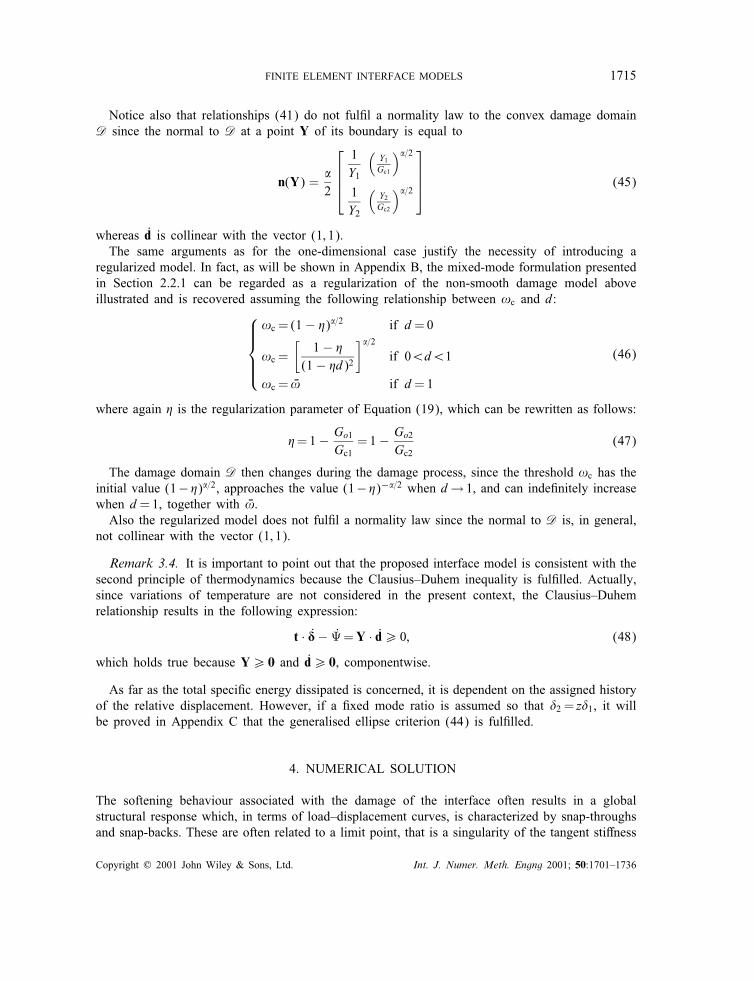
Notice also that relationships (41) do not ful�l a normality law to the convex damage domainD since the normal to D at a point Y of its boundary is equal to

n(Y) =�2

1Y1

(Y1Gc1

)�=2

1Y2

(Y2Gc2

)�=2

(45)

whereas d is collinear with the vector (1; 1).The same arguments as for the one-dimensional case justify the necessity of introducing a

regularized model. In fact, as will be shown in Appendix B, the mixed-mode formulation presentedin Section 2.2.1 can be regarded as a regularization of the non-smooth damage model aboveillustrated and is recovered assuming the following relationship between !c and d:

!c = (1− �)�=2 if d=0

!c =[

1− �(1− �d)2

]�=2if 0¡d¡1

!c = �! if d=1

(46)

where again � is the regularization parameter of Equation (19), which can be rewritten as follows:

�=1− Go1

Gc1= 1− Go2

Gc2(47)

The damage domain D then changes during the damage process, since the threshold !c has theinitial value (1−�)�=2, approaches the value (1−�)−�=2 when d→ 1, and can inde�nitely increasewhen d=1, together with �!.Also the regularized model does not ful�l a normality law since the normal to D is, in general,

not collinear with the vector (1; 1).

Remark 3.4. It is important to point out that the proposed interface model is consistent with thesecond principle of thermodynamics because the Clausius–Duhem inequality is ful�lled. Actually,since variations of temperature are not considered in the present context, the Clausius–Duhemrelationship results in the following expression:

t · T− =Y · d¿ 0; (48)

which holds true because Y¿ 0 and d¿ 0, componentwise.

As far as the total speci�c energy dissipated is concerned, it is dependent on the assigned historyof the relative displacement. However, if a �xed mode ratio is assumed so that �2 = z�1, it willbe proved in Appendix C that the generalised ellipse criterion (44) is ful�lled.

4. NUMERICAL SOLUTION

The softening behaviour associated with the damage of the interface often results in a globalstructural response which, in terms of load–displacement curves, is characterized by snap-throughsand snap-backs. These are often related to a limit point, that is a singularity of the tangent sti�ness



of the �nite element model. Traditional incremental procedures generally fail to overcome theselimit points so that more sophisticated strategies need to be adopted such as the arc length methods.Starting from a pioneering work of Riks [40], who �rst proposed to add to the structural problem

an additional constraint which enforces, at each increment, that a combined norm of the changesof the displacements and of the load (arc length) be equal to a given value, several authors[20; 21; 41–43] developed di�erent versions of the arc length method in order to handle di�erenttypes of non-linear analyses.In particular, problems such as the delamination of composite laminates have the peculiarity that

the non-linear constitutive behaviour can be limited to the small region of the interface where thecrack propagates, while the remaining part of the structure is often modelled as linearly elastic.Even when further non-linearities are introduced in the �nite element model, as when geometricnon-linearity is taken into account or when some damage-plasticity laws for the composite layersare assumed, the presence of limit points in the structural response is still mainly related with thecrack propagation at the interface.This consideration suggested [13; 15; 18] that attention should be focused on those arc length

methods in which the control parameter, which is taken as �xed in the increment, is a functionof a limited set of degrees of freedom (local control), namely the ones which are directly relatedto the non-linear behaviour, in this case the relative displacements in the interface elements at thedelamination front.Accordingly, this approach was initially followed by adopting the local control procedure il-

lustrated in Reference [44], a method which is close to that proposed in References [13; 18].However, some preliminary numerical results, which have been presented in Reference [45], in-dicated that the method was less robust than the quadratical arc length [27; 28], in its modi�edform recently presented in References [29; 30]. The latter method has therefore been used for thecurrent numerical applications. Nevertheless, the possibility of improving the numerical stabilityand the convergence rate via a local control procedure needs further investigation and will be thesubject of future work.Referring to the above-quoted references, for major details, let us brie y recall that in the kth

iteration, within a generic increment of the full Newton method, the following equation is solved:

Kkt �p

k = �k+1qe − qi(pk) = gk + ��kqe; k = 0; 1; : : :

where Kkt is the structural sti�ness matrix, �p

k is the change of the displacements in the iteration,qi(pk) is the vector of the internal forces, �k+1 = �k + ��k is the load multiplier, at the end of theiteration, of the external force vector qe (proportional loading is assumed), and gk = �kqe− qi(pk)is the residual force vector at the beginning of the kth iteration.Accordingly, the superscript 0 will denote the values obtained after reaching convergence at the

previous increment, and the total change �pk+1 = pk+1 − p0 is written as follows:

�pk+1 =�pk + � �pk + ��k�pkt (49)

where the vectors � �pk = [Kkt ]

−1gk and �pkt = [Kkt ]

−1qe are usually referred to as the iterative andtangential displacements, respectively, while ��k = �k+1 − �k is the unknown change of the loadfactor.In the quadratic arc length the following equation is added as an additional constraint:

‖�pk+1‖=�l (50)



The arc length �l is assumed as �xed in the increment whereas an automatic incrementationprocedure is used to update its value at increment i + 1, known the value at increment i, via theformula

�li+1 =

√IdIp�li (51)

where Ip is the number of iterations required for getting convergence at increment i and Id is auser de�ned number of ‘desired’ iterations.Two di�erent issues arise at the �rst ‘predictor’ iteration (k =0) and during the next, possible,

‘corrector’ ones (k¿1). At the �rst iteration, Equations (49) and (50) yield

��o= �1 − �o= ± �l‖�p0t ‖

(52)

Di�erent methods have been proposed for choosing the sign in Equation (52), see References[28; 30]. In the numerical applications carried out, no problems of bifurcation have been encoun-tered and then the same sign has been taken as that of the determinant of the sti�ness matrix,which can approximately be evaluated by considering the number of negative pivots resulting fromthe factorization of Kt .At the corrector iterations Equation (50) results in a quadratic equation in ��k which, in gen-

eral, will give two real or imaginary roots ��1k and ��2k . The latter case, which has rarely beenexperienced during the numerical applications for the intereface model, is a warning for a toolarge increment size �l. The analysis must then be restarted from the last converged incrementbut with a reduced arc length.In the usual case when the roots are real, two di�erent values pk+11 (��k

1) and pk+12 (��k

2) of thedisplacement vector are associated with them:

pk+1j (��kj )= p

0 + �pk + � �pk + ��kj �p

kt ; j=1; 2 (53)

For problems characterized by relatively smooth limit points, the ‘angle-criterion’ is generallyadopted. With this approach, one computes the two angles between the new incremental changesof p, �pk+1j = pk+1j (��k

j )− p0, and the incremental change at the beginning of the iteration, �pk .The value of ��k

j which corresponds to the minimum of such angles is then chosen.However, in the examples presented in this paper, it has proved fundamental to follow the

procedure recently proposed in Reference [29], see also Reference [30], that is to choose the rootwhich provides the minimum residual norm ‖gk+1‖. In fact, this method is necessary when sharpsnap-backs are encountered in the structural response. As will be shown by several numericalexamples, this is the case of the delamination analysis where sharp snap-backs can be either a realcharacteristic of the structural response or the result of spurious oscillation related to an insu�cientmesh re�nement around the crack front.The key idea underneath the criterion for choosing the root is illustrated in Figure 9. Strictly,

it refers to a one-dimensional case and to the so-called ‘spherical’ arc length method [28], inwhich the change of � is also added in the constraint equation, since in that case the concept cangraphically be explained more easily.



Figure 9. Minimum residual criterion for the choiceof the root.

Figure 10. Material sti�ness at the predictor.

4.1. Iterative matrix at the predictor

Let us consider a point of the interface at which, during the generic increment i, the delaminationprocess is developing so that the last converged value of the damage parameter d, dci , is greaterthan the one, d0i , at the beginning of the increment, being 0¡dci¡1. In this case, in terms of thedamage parameter � , at the beginning of the next increment, i + 1, it turns out to be 0i+1 = �

0i+1

and then, in accordance with Equation (17), the tangent constitutive operator is used to form thesti�ness matrix, computed via (17)2.This is not straightforward because it is not known in advance whether at that point, during

the new increment, i + 1, unloading or further delamination is going to occur. In the latter caseexpression (17)2 gives the best predictor material sti�ness, whereas in the former case the secantmaterial sti�ness provided by expression (17)3 is more appropriate, see also Figure 10, whichrefers to a one-dimensional case.A similar issue appears in other contexts, such as in elastoplasticity when, at the beginning

of an increment, the stress at the Gauss point under examination relies on the boundary of theelastic domain. In this latter case some analysts recommend that an elastic behaviour is to bea priori assumed, leaving the use of the tangent operator for the next corrector iterations, ifnecessary. Although it seems to be theoretically impossible to �nd out a general optimal strategyfor addressing an issue which is problem dependent, in Reference [46] it has been shown that,for a general class of elastoplastic problems, the choice of the tangent operator at the predictoriteration results in enhanced convergence properties of the solution algorithm.As will be detailed later, a similar result has also been obtained in the present context for the

analysis of delamination and the numerical results presented show that not only is the convergencerate improved if the tangent material sti�ness at the predictor is assumed instead of the secant onebut, more important, the robustness of the solution algorithm is signi�cantly enhanced.Although a deeper investigation for cases like cyclic load histories is probably needed to con�rm

the general validity of this last statement, it appears that a point which is currently undergoingdelamination during one increment is likely to be subject to further damage in the next one.Furthermore, the increased robustness, which is even more signi�cant than the improvement of theconvergence rate, is probably related with the strategy adopted for overcoming the limit points,



since the choice of a secant or of a tangent constitutive operator often results in a positive ornegative determinant of the structural sti�ness matrix and, therefore, in a di�erent sign of thepredictor change of the load factor in Equation (52).

4.2. Numerical integration in the interface elements

A peculiarity of the interface model is the fact that the Gauss rule is not recommended for thenumerical integration of the tangent sti�ness matrix and the internal force vector of the interfaceelements [14; 31–35].This issue has been speci�cally discussed in Reference [31], where an explanation has been

provided for some numerical results presented in some papers, mainly related to the use of interfaceelements for the analysis of geomechanics or concrete problems [32–34], which show a superiorperformance of the Newton–Cotes integration rule with respect to the Gauss quadrature commonlyadopted for the 2D and 3D continuum elements. In Reference [31] it has been shown that, for linearelements, the application of Gauss quadrature results in a coupling between the degrees of freedomof di�erent node sets and then in an oscillation of the traction pro�le, for high values of the tractiongradients, which is not recovered if a Newton–Cotes integration rule is used. Similar results arealso found for quadratic elements although in that case some more detailed considerations need tobe made.Furthermore, because of the non-smooth pro�le of the stress in an element which is only partially

delaminated, a high number of integration points might yield a more accurate estimation of thesti�ness and of the residual forces [14; 35]. However, some numerical results that will be presentedhere suggest that the increased stress accuracy does not necessarily allow the use of a coarsermesh and indeed the overall robustness of the solution algorithm can be negatively in uenced. Asa result, if the mesh is not su�ciently re�ned around the delamination front the spurious jumpsof the load=displacement curves still remain but, in addition, the average increment size evaluatedby the automatic incrementation procedure is considerably reduced.

5. NUMERICAL RESULTS

The interface model described in the previous sections has been implemented in a research versionof the �nite element code LUSAS [47].In this section some numerical results will be presented and discussed for two di�erent analyses

of mode 1 and mixed-mode delamination. A comparison is also made with the results obtainedusing the virtual crack closure method [1–3], that is a direct application of LEFM, and withavailable experimental data [8; 48].

5.1. Numerical simulation of a DCB test

As a pure mode 1 problem a double cantiliver beam has been analysed under displacement control.The geometry is described in Figure 11 and the material data are given in Table I. Strictly, a 3Danalysis would be needed since the delamination front is not precisely a straight line. Indeedin earlier work by the second author [22] a three-dimensional analysis was applied. The resultsindicated that the 2D plane strain formulation gave a very reasonable approximation.First, a regular mesh of 4× 400 eight-node plane strain (Q8) elements and 280 six-node interface

(INT6) elements has been adopted. In Figure 12 the vertical reaction at point P has been plotted



Figure 11. DCB: geometry.

Table I. DCB specimen: material data.

Composite

E11(GPa) E22 =E33(GPa) G12(GPa) �12 = �13 �23135.3 9.0 5.2 0.24 0.46

Interface

Gc(Nmm−1) �o to(MPa)0.28 10−7 57.0

Figure 12. DCB: reaction at P vs prescribed displacement.

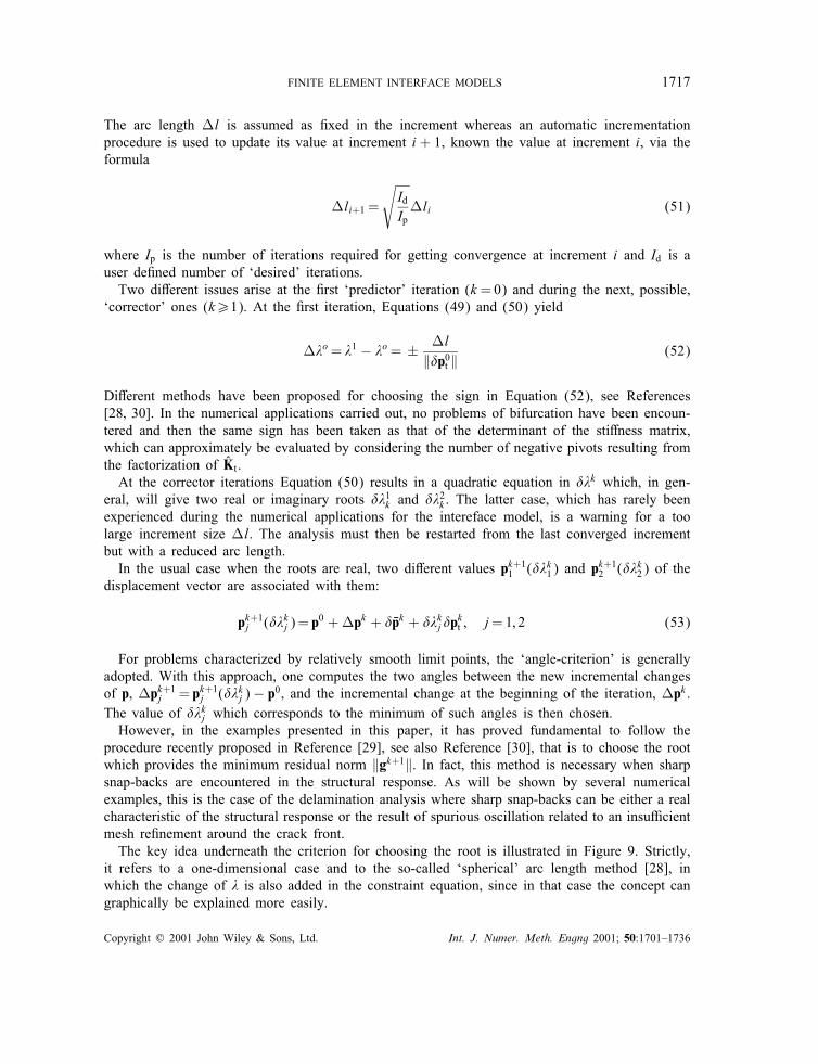
against the vertical displacement u for the interface model and the VCC method. It is worth notingthat the load–displacement curves for DCB analyses presented in the literature often refer to therelative displacement between the two points on the left of Figure 11 where the displacements areprescribed. The latter would be equal to 2u.In Figures 13 the results of a sensitivity analysis to the tensile strength have been presented.

The spurious oscillations show that, for a value of to=57MPa, the mesh used is too coarse andFigures 14 show the improvements obtained by re�ning the mesh. Notice, however, the increase ofthe necessary number of increments. It can be seen that the solution obtained with the low tensilestrength (to=1:7MPa) is in good agreement with the VCC solution for the late propagation phasebut the solution is much too exible in the early loading stages. The later example with mixed-mode fracture will show that this early discrepancy can, for some problems, lead to misleadingresults even in the later loading stages.



Figure 13. (a) DCB: di�erent to; (b) DCB: di�erent to (zoom).

Figure 14. (a) DCB: di�erent meshes, to = 57:0MPa; (b) DCB: di�erent meshes, to = 57:0MPa (zoom).

Next, the in uence of the material sti�ness used at the predictor iteration is studied. The twomethods discussed in Section 4.1 will be referred to as ‘tangent predictor’ and ‘secant predictor’procedures.Figure 15(a) refers to the mesh with 4× 100 Q8 elements, with 70 six-node interface elements,

and to a tensile strength of to=1:7MPa. The response is relatively smooth since it is characterizedby one snap-through and no snap-backs.In this case both procedures are robust but the superiority of the tangent predictor is testi�ed

by the improved rate of convergence which results in a reduced number of iterations with respectto the one required for the secant predictor method.In fact, in accordance with the automatic incrementation procedure adopted, see Equation (51),

the improved convergence also yields an increase of the average increment size and then of thearc length �l.A more important feature of the tangent predictor procedure is its satisfactory robustness even

when very sharp snap-throughs and snap-backs are encontoured. The curves in Figure 15(b) have



Figure 15. (a) Response with t0 = 1:7MPa; (b) Response with t0 = 57:0MPa.

Figure 16. (a) Di�erent number of integration points; (b) di�erent number of integration points (zoom).

been obtained with to=57:0MPa. It shows a case in which several snap-backs are due to a coarsemesh rather than to the real structural behaviour.One may argue that the problem of having sharp snap-backs can be solved by re�ning the mesh.

In this sense, a criterion which relates the optimal mesh size to the adopted interface strength wouldbe very useful and future work will address this issue. In the meantime it is desirable to havean algorithm which overcomes the limit points without falling into a ‘black hole’, as happens forthe secant predictor strategy in the case of Figure 15(b), so that a preliminary analysis can besuccessfully completed even with a coarse mesh. Furthermore, sharp snap-backs can be the resultof the actual structural behaviour, as will be shown later for a mixed-mode, multiple delamination.The in uence of the number of points used for evaluating the sti�ness matrix and the residual

force vector in the interface elements can be seen from Figure 16 which refers to a mesh of4 × 100 plane strain elements enriched with enhanced strains (Q4M) and 70 linear interfaceelements (INT4) with a tensile strength of 32:0MPa. Simpson rule has been used with 2 and 20points and it is apparent that the increase of the number of integration points results in an increase



Figure 17. (a) 20 points vs 2 points with umax = 0:05mm; (b) 20 points vs 2 pointswith umax = 0:05mm (zoom).

Figure 18. (a) Results with two integration points; (b) results with two integration points (zoom).

of the number of spurious oscillations of the reaction=displacement curve. In fact, for a highernumber of integration points, the solution algorithm turns out to be less robust and the automaticincrementation procedure considerably reduces the step. Conversely, the higher stability achievedwith two quadrature points allows for a larger average step size so that the solution often managesto ‘jump over’ several ‘bumps’.In Figure 17 a curve has been obtained using two integration points but �xing a maximum value

�umax = 0:05mm for the change of the applied displacement in each increment. In this case thesolution cannot ‘jump over the bumps’ and the result is similar to the one obtained with 20 points.This means that the frequency of the bumps in the real solution is indeed independent from thenumber of integration points, and that the reduced number obtained in Figure 16 for two pointsis related to the increased stability.Furthermore, in order to investigate the general validity of the result, a small perturbation has

been introduced by assigning, in the data of the interface, a di�erent value of �o equal to 10−6

and 10−7, respectively. The curves obtained, plotted in Figure 18, are di�erent, but the general



Figure 19. Contour-plot of �y for to = 57:0MPa (uP = 2:66mm).

Figure 20. Contour-plot of �y for to=1:7MPa (uP = 2:55mm).

trend is similar and then the ability of ‘jumping over the bumps’ seems to be related with a higherstability rather than with pure luck. As a conclusion, increasing the number of integration pointsdoes not seem to be equivalent to a mesh re�nement.Figures 19 and 20 show the contour-plots of the component �y of the stress in the composite

for a mesh of 4 × 400 Q4M and 280 INT4 elements and tensile strengths of 57.0 and 1:7MPa,respectively.They con�rm that, in terms of the stress �eld, the solution is strongly dependent on the tensile

strength, as one could expect. In contrast, the results in terms of load=displacement curves suggestthat, for low values of to, a good agreement can be still obtained between the interface model andthe LEFM formulation. However, this does not allow one to arbitrarily reduce the strength since,below a certain value, incorrect results can be obtained also in terms of the load=displacementcurves. This is clearly shown for the more complex case of multiple delamination which will beaddressed later on in this section.Figure 21 shows a comparison between the load–displacement curves obtained with the use of

linear 4-node interface elements (INT4) and Q4M parent elements and the ones resulting fromusing quadratic 6-node interface elements (INT6) with Q8 parent elements. Two di�erent meshes



Figure 21. (a) Linear and quadratic elements: to=32:0MPa; (b) linear and quadratic elements: to=57:0MPa.

have been used which have a comparable number of nodes. For a lower value of the tensilestrength, to=32:0MPa, the linear elements are more e�cient, whereas in case of a higher tensilestrength, to=57:0MPa, the performances of the quadratic elements are more satisfactory. Thisobservation contrasts somewhat with the conclusion in Reference [21] that linear elements aremore e�ective.In this respect, it is worth noting that, when using the quadratic elements, the Simpson integration

rule has been adopted to produce the results presented in this paper. Several numerical simulationsrevealed that the Newton–Cotes and the Simpson rule, with three points per element in both cases,can give di�erent results in terms of stability and convergence rate, but it appears that no generalrule can be deduced to predict in advance which one of them is the most convenient.In order to compare the numerical results with an analytical solution [37], the same DCB has

been studied considering an isotropic material with Young modulus E=2:1×105 MPa and Poissonratio �=0:3. A regular mesh of 4 × 400 four-node plane strain elements and 70 INT4 elementshas been assumed.Two analyses have been carried out using, for the �rst one, ordinary plane strain elements (Q4)

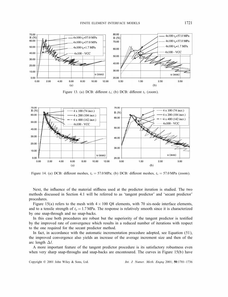
and, for the second one, plane strain elements enriched with enhanced strains (Q4M). Figure 22shows the importance of adding the enhanced modes to avoid shear-locking phenomena as wellas a good agreement of the interface element model and the VCC method with the analyticalsolution.In Figure 23 we show a comparison between the results of the interface damage model and

some available experimental results provided in Reference [48]. In this case the composite is aXAS-913C, a carbon �bre epoxy composite whose material data are reported in Table II, andthe geometry of the DCB specimen is the same as in Figure 11, except for the width which isnow 30mm. The agreement is good.

5.2. Mixed-mode multidelamination analysis

A case of multiple delamination has been analysed under displacement control. The geometry andthe load conditions are illustrated in Figure 24 and the material data are given in Table III. Theycorrespond to a (024) unidirectional HTA913 carbon-epoxy composite.



Figure 22. Isotropic material: comparison with ananalytical solution.

Figure 23. Comparison with experimental data re-ported in Reference [48].

Table II. DCB specimen: material data reported in Reference [48].

Composite XAS-913C

E11(GPa) E22 =E33(GPa) G12(GPa) �12 = �13 = �23126 7.5 4.981 0.263

Interface

Gc(Nmm−1) �o to(MPa)0.281 10−6 57.0

Table III. Multiple delamination analysis: material data.

Composite

E11(GPa) E22 =E33(GPa) G12(GPa) �12 = �13 �23115.0 8.5 4.5 0.29 0.3

Interface

Gc1(Nmm−1) Gc2(Nmm−1) 1− � � to1(MPa) to2(MPa)0.33 0.80 1.0e−6 2 3.3 7.0

Figure 24. Multiple delamination analysis: geometry.



Figure 25. Reaction at P against prescribeddisplacement.

Figure 26. Comparison with the VCC method.

Two initial cracks are assigned. The one on the left is positioned at the middle plane of thespecimen. The second one is positioned on the right of the �rst one, two layers beneath. Theinterface elements have been inserted at the not-initially delaminated parts of the interfaces betweenthe 10th and the 11th layers and between the 12th and the 13th layers, starting from below.A regular mesh of 3 × 360Q4M elements and 680 INT4 interface elements has been used. In

Figure 25 the reaction at the point P is plotted against the prescribed displacement. It shows agood agreement between the results of the interface model and the experimental data taken fromReference [8], as well as the failure of the secant predictor method in successfully completing theanalysis.The �rst part the curves of Figure 25 are almost linear with the slight non-linearity being due to

the fact that some points immediately ahead of the upper initial crack are in the softening regionalthough no one of them is completely delaminated before the point A has been reached.Between points A and B the behaviour is approximately typical of a DCB specimen and,

accordingly, only mode 1 is activated. Point B corresponds to a position of the crack tip whichis approximately 10mm before the second initial crack. The presence of the second initial cracknow in uences the delamination process, although only the upper crack propagates until point Cin the curve is reached, which corresponds to a position of the upper crack approximately abovethe mid-point of the second initial crack. The numerical analysis predicts an extra local limit pointthat is not immediately obvious from the experimental results and might be an artefact of themesh.Starting from point C, the second initial crack propagates to the right and the two cracks grow

simultaneously, the lower one moving approximately twice as fast as the upper one. A mixed-modedelamination occurs at this stage, although mode 1 is still more signi�cant.In Figure 26 a comparison is made between the results of the interface model and the curve

obtained via the application of VCC. In this case of multiple delamination, for the VCC method,the energy release rates associated with the two cracks are evaluated at each step. Then the crackwhich is associated with the higher value of G1=Gc1 + G2=Gc2 is moved, and the load multiplieris computed so as to ful�l the linear criterion (9). It is worth noting that the curve obtained by



Figure 27. Multidelamination analysis: def. mesh and contour-plot of �y.

applying the VCC method shows a discontinuous trend in the part corresponding to the multipledelamination process. In fact, the simple implementation of the VCC method does not allowfor a real simultaneous advance of both cracks so that, to circumvent this drawback, adaptiveremeshing procedures should be used at each increment [8], with an increase of the computationalburden.Furthermore, in Figure 26 the curve obtained by reducing the strengths to to1 = 0:66MPa and

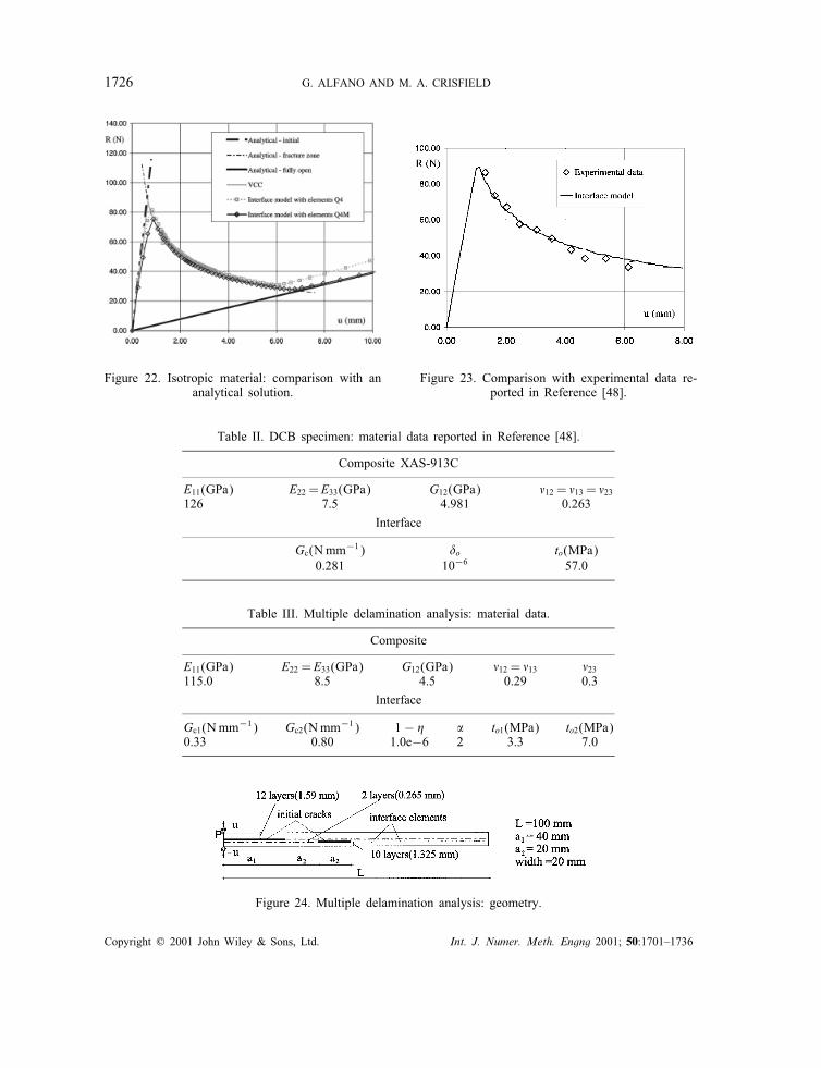
to2 = 1:6MPa has been plotted. It shows that, if excessively low values of the strengths are assumed,the results can become unreliable.In Figure 27 the deformed mesh and the contour-plot of the component �y in the composite are

shown for a value u=37:2mm of the prescribed displacement.

6. CONCLUSIONS

The numerical analysis of the delamination in laminated composites has been addressed startingfrom an interface damage model originally presented in References [20–22]. The mixed-mode for-mulation has been modi�ed to circumvent the inconsistency of reaching complete delamination inmodes 1 and 2 at a di�erent time. The model allows one to simulate the mixed-mode delamina-tion without any hypotheses on the mode ratio so that no ‘pre-solution’ analyses are needed. Thisis because the interface relationship satis�es a generalized propagation criterion, introduced inReferences [20–22], which encompasses two criteria proposed in References [23; 24], often usedin practical applications.It has then been shown that the model can be recovered in the context of a damage mechanics

theory as a regularization of a non-smooth model. The non-smooth model, in turn, reproducesthe results of traditional fracture mechanics approaches when the penalty sti�eness parameters,introduced to properly simulate the pre-crack behaviour, tend to in�nity. In the framework ofdamage mechanics an alternative proof that the model satis�es the generalized mixed-mode criterionhas been provided.



Some issues related with the numerical solution of the structural problem have been studied. Thestructural response is often characterized by sharp snap-throughs and snap-backs, which can eitherbe due to the real behaviour of the structure or be a result of a �nite element mesh not re�nedenough around the delamination front. In both cases it is important that the solution procedurebe able to overcome these limit points and the strategy proposed in References [29; 30], as amodi�cation of the quadratic arc length [27; 28], has proved to be the most robust so far, althoughfurther investigations on local control arc length procedures will be the object of future work.The importance of using the tangent material sti�ness in the predictor iteration at a point which

has undergone delamination in the previous increment has been pointed out. This choice is con-sistent with an hypothesis of further delamination in the new increment and the numerical resultspresented show the improved rate of convergence and the enhanced numerical stability with respectto the case in which the secant material sti�ness is used, which would be in accordance with anhypothesis of unloading.Some of the numerical results presented have shown that increasing the number of integration

points in the interface elements, in order to get a more accurate estimation of the tangent sti�nessmatrix and of the residual force vector, can reduce the stability of the solution algorithm. As aresult, the undesired oscillations of the response for a coarse mesh are not eliminated whereas thenumber of required increments increases.The sensitivity of the model to the interface strength has then been investigated. Reducing the

values of the maximum admissible tractions lighten the computational burden because it allowsfor a coarser mesh around the crack tip and an increased average increment size. However, toosmall values can result in unacceptable errors and should be avoided.The extension of the current treatment to the 3D case is quite simple and results will be

presented in forthcoming papers. It can be accomplished by replacing the line interface elementwith a surface element and introducing mode III in the formulation, which is to be treacted thesame way as mode II although it is generally characterised by di�erent material properties (inparticular it may be that GcII 6=GcIII). In this respect it is worth noting that the 3D formulationcan also be used for the analysis of delamination in plate and shell structures. Indeed many recent�nite element formulations for shells discard rotations and use ‘brick-like’ elements in which thevariables at the top and bottom nodes are assumed as unknowns.

APPENDIX A: DERIVATION OF THE INTERFACE MODEL FROM A DAMAGEMECHANICS THEORY: SINGLE-MODE DELAMINATION

Hereafter we show that the interface model described by Equation (4) can be recovered by usingthe damage mechanics formulation given by Equations (26)–(28) if relationship Equation (32) isassumed to hold true.To this end, let us rewrite Equation (4) eliminating, for the sake of simplicity, any sign or

component issues, analogously as in Section 3.1:

t=

K� if �max 6 �o[1−

(�max − �o

�max

)�c

�c − �o

]K� if �o¡�max¡�c

0 if �max ¿ �c

(A1)



Let us observe that

�max¡�o ⇔ �Y = 12K�2max¡Go= 1

2K�2o

Accordingly, if one initially sets Yc =Go for d=0, Khun–Tucker conditions (27) ensure that d=0as long as �max¡�o, so that (26)1 is equivalent to (A1)1. For �max = �o we get �Y =Go, whichallows d¿ 0. Then, for d=0, (26)1 is still equivalent to (A1)1, whereas as soon as d¿0, (32)2has to be considered.Since for 0¡d¡1 we are in the softening part of the interface law, one can equate the expression

of the traction in Equation (26)1 to that given by Equation (A1)2:

t=(1− d)K�=[1−

(�max − �o

�max

)�c

�c − �o

]K� (A2)

Hence, by making use of the relationships

�c�c − �o

=Gc

Gc − Go

�o

�max=

√2Go=K√2 �Y =K

=

√Go

�Y(A3)

one gets

d =Gc

Gc − Go

(1− �o

�max

)=

GcGc − Go

(1−

√Go

�Y

)(A4)

and inverting

�Y =Go

(1− ((Gc − Go)=Gc )d)2(A5)

Substituting the right-hand side of (32)2 into (27), we get

Y 6Go

(1− ((Gc − Go)=Gc )d)2d¿ 0

(Y − Go

(1− ((Gc − Go)=Gc )d)2

)· d = 0 (A6)

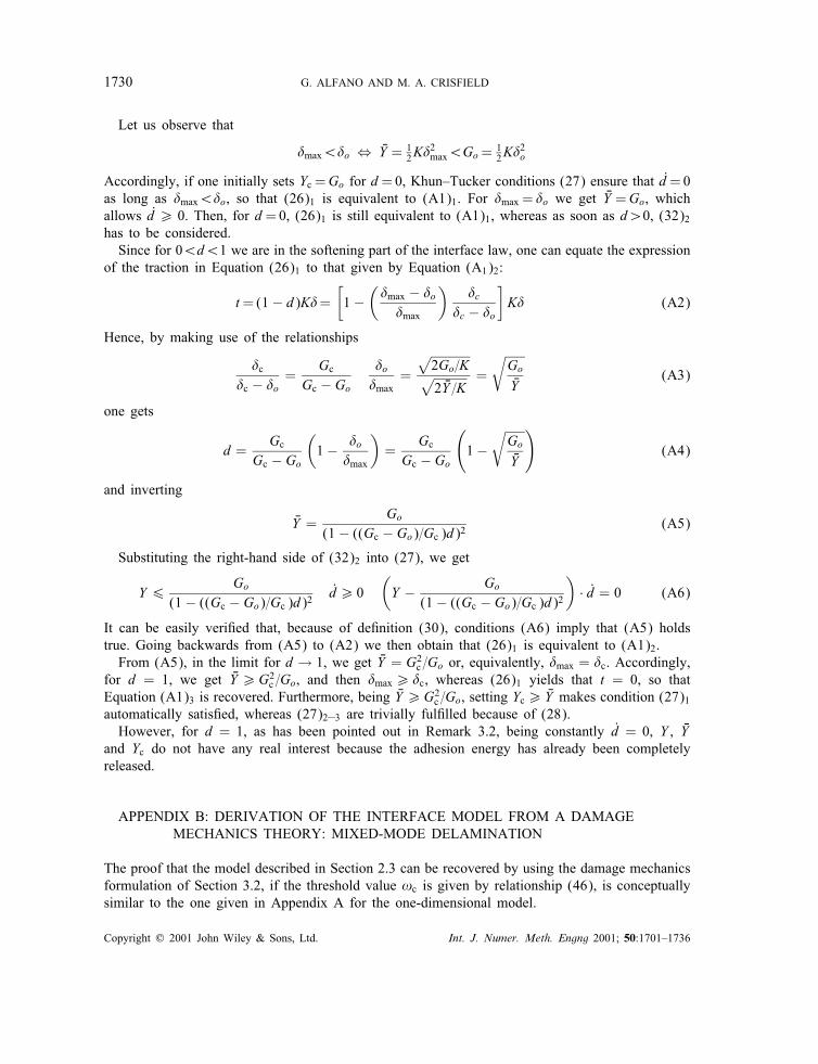
It can be easily veri�ed that, because of de�nition (30), conditions (A6) imply that (A5) holdstrue. Going backwards from (A5) to (A2) we then obtain that (26)1 is equivalent to (A1)2.From (A5), in the limit for d → 1, we get �Y = G2c =Go or, equivalently, �max = �c. Accordingly,

for d = 1, we get �Y ¿G2c =Go, and then �max¿ �c, whereas (26)1 yields that t = 0, so thatEquation (A1)3 is recovered. Furthermore, being �Y ¿G2c =Go, setting Yc¿ �Y makes condition (27)1automatically satis�ed, whereas (27)2–3 are trivially ful�lled because of (28).However, for d = 1, as has been pointed out in Remark 3.2, being constantly d = 0, Y , �Y

and Yc do not have any real interest because the adhesion energy has already been completelyreleased.

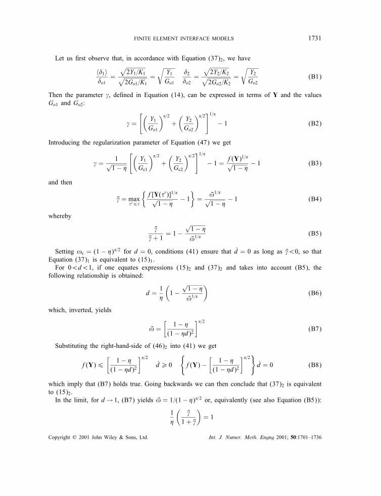
APPENDIX B: DERIVATION OF THE INTERFACE MODEL FROM A DAMAGEMECHANICS THEORY: MIXED-MODE DELAMINATION

The proof that the model described in Section 2.3 can be recovered by using the damage mechanicsformulation of Section 3.2, if the threshold value !c is given by relationship (46), is conceptuallysimilar to the one given in Appendix A for the one-dimensional model.



Let us �rst observe that, in accordance with Equation (37)2, we have

〈�1〉�o1

=

√2Y1=K1√2Go1=K1

=

√Y1Go1

�2�o2

=

√2Y2=K2√2Go2=K2

=

√Y2Go2

(B1)

Then the parameter , de�ned in Equation (14), can be expressed in terms of Y and the valuesGo1 and Go2:

=

[(Y1Go1

)�=2

+(

Y2Go2

)�=2]1=�

− 1 (B2)

Introducing the regularization parameter of Equation (47) we get

=1√1− �

[(Y1Gc1

)�=2

+(

Y2Gc2

)�=2]1=�

− 1 = f(Y)1=�√1− �

− 1 (B3)

and then

� = max�′6�

{f[Y(�′)]1=�√

1− �− 1}=

�!1=�√1− �

− 1 (B4)

whereby

� � + 1

= 1−√1− �

�!1=�(B5)

Setting !c = (1 − �)�=2 for d = 0, conditions (41) ensure that d = 0 as long as � ¡0, so thatEquation (37)1 is equivalent to (15)1.For 0¡d¡1, if one equates expressions (15)2 and (37)2 and takes into account (B5), the

following relationship is obtained:

d =1�

(1−

√1− �

�!1=�

)(B6)

which, inverted, yields

�! =[

1− �(1− �d)2

]�=2(B7)

Substituting the right-hand-side of (46)2 into (41) we get

f(Y)6[

1− �(1− �d)2

]�=2d¿ 0

{f(Y)−

[1− �

(1− �d)2

]�=2}d = 0 (B8)

which imply that (B7) holds true. Going backwards we can then conclude that (37)2 is equivalentto (15)2.In the limit, for d→ 1, (B7) yields �! = 1=(1− �)�=2 or, equivalently (see also Equation (B5)):

1�

(�

1 + �

)= 1



Hence, for d = 1, �!¿ 1=(1−�)�=2 and (1=�) (� =(1 + � ))¿ 1, whereas Equation (37)1 yields t = 0,so that Equations (20) and (21) are recovered.Furthermore, since it is �!¿ (1 − �)�=2, setting !c = �! makes condition (41)1 automatically

satis�ed whereas (41)2–3 are ful�lled because of (28).

APPENDIX C: FULFILLMENT OF THE GENERALIZED ELLIPSE CRITERION:DAMAGE MECHANICS APPROACH

We here show that, if a proportional history of relative displacement is assigned, so that

�2 = z�1 (C1)

the GEC (11) is ful�lled.Considering only the case �1¿0, let us observe that, using (C1), we can write

Y2 = pY1 (C2)

with p = z2K2=K1. Furthermore, we can rule out the case in which

�!¿(

Y1Gc1

)�=2

+(

Y2Gc2

)�=2

because it would yield d = 0. Therefore we consider, without loss of generality, a monotonicloading so that

�! = f(Y) =(

Y1Gc1

)�=2

+(

Y2Gc2

)�=2

(C3)

By di�erentiating Equation (B6), we then get

dddYi

=√1− ��

1

2G�=2ci

Y �=2−1i

f(Y)1=�+1(C4)

and exploiting (C2) we can write

∫ +∞

0Y1d1 dt =

∫ Y ′′1

Y ′1

Y1dd1dY

· dY

=√1− ��

∫ Y ′′1

Y ′1

12f(Y)1=�+1

[(Y1Gc1

)�=2

dY1 +

(Y1Y

�=2−12

G�=2c2

)dY2

]

=√1− �� a

∫ Y ′′1

Y ′1

12√Y1dY1 =

√1− �� a

[√Y1]

Y ′′1

Y ′1

(C5)

having set

a =

[(1

Gc1

)�=2

+(

pGc2

)�=2]1=�



To obtain the integration limits Y ′1 and Y ′′

1 let us write Equation (B7) using (C2) and (C3):

�! =(

Y1Gc1

)�=2

+(

Y2Gc2

)�=2

= Y �=21

[(1

Gc1

)�=2

+(

pGc2

)�=2]

= Y �=21 a� =

[1− �

(1− �d)2

]�=2(C6)

Setting d = 0 and 1, respectively, one gets

Y ′1 =

1− �a2

; Y ′′1 =

1(1− �)a2

(C7)

We then obtain ∫ +∞

0Y1d1 dt

Gc1=

√1− �

� aGc1

(1

a√1− �

−√1− �a

)=

1a2Gc1

(C8)

Analogously we derive that ∫ +∞

0Y2d2 dt

Gc2=

pa2Gc2

(C9)

so that we �nally get

∫ +∞

0Y1 · d1 dtGc1

�=2

+

∫ +∞

0Y2 · d2 dtGc2

�=2

=1a�

[(1

Gc1

)�=2+(

pGc1

)�=2]= 1 (C10)

APPENDIX D: FULFILLMENT OF THE GENERALIZED ELLIPSE CRITERION:DIRECT APPROACH

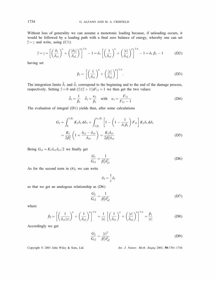
We report here an alternative proof of the result given in Appendix C, originally given in theinternal report [37], which is based on the formulation presented in Section 2, allowing for di�er-ent ratios �oi=�ci for the di�erent modes and removing the hypothesis that �o1 = �o2, assumed inReference [37].We want to prove that Equation (11) is ful�lled if the proportional relative displacement history

(C1) is assumed, with z �xed during the delamination process, and the interface relationship ofSection 2.2 is adopted. However, expressions (6) will now be used and substituted into (11).Hence, let us consider expression (6)1, assuming that �1¿0. From relationships (15) we can

split the integral in two parts:

G1 =∫ �1

0K1�1 d�1 +

∫ �1

�1

(1− �

� + 1F11

)K1�1 d�1 (D1)



Without loss of generality we can assume a monotonic loading because, if unloading occurs, itwould be followed by a loading path with a �nal zero balance of energy, whereby one can set� = and write, using (C1):

� = =[(

�1�o1

)�

+( |�2|

�o2

)�]1=�− 1= �1

[(1�o1

)�

+( |z|�o2

)�]1=�− 1= �1 �1 − 1 (D2)

having set

�1 =[(

1�o1

)�

+( |z|�o2

)�]1=�: (D3)

The integration limits �1 and �1 correspond to the beginning and to the end of the damage process,respectively. Setting � =0 and (� =(� + 1))F11 = 1 we then get the two values:

�1 =1�1

�1 =�1�1

with �1 =F11

F11 − 1 (D4)

The evaluation of integral (D1) yields then, after some calculations

G1 =∫ 1=�1

0K1�1 d�1 +

∫ �1=�1

1=�1

[1−

(1− 1

�1�1

)F11

]K1�1 d�1

=K12�21

(1 +

�c1 − �o1

�o1

)=

K1�c12�21�o1

(D5)

Being Gc1 =K1�o1�c1=2 we �nally get

G1Gc1

=1

�21�2o1

(D6)

As for the second term in (6), we can write

�2 =1z�1

so that we get an analogous relationship as (D6)

G2Gc2

=1

�22�2o2

(D7)

where

�2 =[(

1�o1|z|

)�

+(1�o2

)�]1=�=1|z|[(

1�o1

)�

+( |z|�o2

)�]1=�=

�1|z| (D8)

Accordingly we get

G2Gc2

=|z|2�21�

2o2

(D9)



and then(G1Gc1

)�=2+(

G2Gc2

)�=2=(

1�21�

2o1

)�=2+

(|z|2�21�

2o2

)�=2=1��1

[(1�o1

)�

+( |z|�o2

)�]=1 (D10)

which is the desired result.

ACKNOWLEDGEMENTS

The work has been supported by an EPSRC grant. The authors would like to thank FEA Ltd. for providingthe �nite element computer program LUSAS.

REFERENCES

1. Irwin GR. Analysis of stresses and strains near the end of a crack transversing a plate. Journal of Applied Mechanics1957; 24:361–366.

2. Rybicki EF, Kanninen MF. A �nite element calculation of stress intensity factors by a modi�ed crack closure integral.Engineering Fracture Mechanics 1977; 9:931–938.

3. Raju IS. Calculation of strain-energy release rates with higher order and singular �nite elements. Engineering FractureMechanics 1987; 28(3):251–274.

4. Rice JR. A path independent integral and the approximate analysis of strain concentration by notches and cracks.Journal of Applied Mechanics 1968; 35:379–386.

5. Hellen TK. On the method of the virtual crack extension. International Journal for Numerical Methods in Engineering1975; 9:187–207.

6. Parks DM. A sti�ness derivative �nite element technique for determination of crack tip stress intensity factors.International Journal of Fracture 1974; 10(4):487–502.

7. Gri�th AA. The phenomena of rupture and ow in solids. Philosophical Transactions of the Royal Society, London;Series A 1921; 221:163–198.

8. Robinson P, Besant T, Hitchings D. Delamination growth prediction using a �nite element approach. 2nd ESIS TC4Conference on Polymers and Composites, Les Diablerets, Switzerland, 1999.

9. Hilleborg A, Modeer M, Peterson PE. Analysis of crack formation and growth in concrete by means of fracturemechanics and �nite elements. Cement and Concrete Research 1976; 6:773–782.

10. Tvergaard V, Hutchinson JW. The in uence of plasticity on mixed-mode interface toughness. Journal of the Mechanicsand Physics of Solids 1993; 41:1119–1135.

11. Yueguang W, Hutchinson JW. Interface strength, work of adhesion and plasticity in the peel test. International Journalof Fracture 1998; 93:315–333.

12. Allix O, Ladeveze P, Corigliano A. Damage analysis of interlaminar fracture specimens. Composite Structures 1995;31:66–74.

13. Allix O, Corigliano A. Modeling and simulation of crack propagation in mixed-modes interlaminar fracture specimens.International Journal of Fracture 1996; 77:111–140.

14. Point N, Sacco E. A delamination model for laminated composites. International Journal of Solids and Structures1996; 33(4):483–509.

15. Schellekens JCJ, De Borst R. A Non-linear �nite element approach for the analysis of mode I free edge delaminationin composites. International Journal of Solids and Structures 1993; 30(9):1239–1253.

16. Bruno D, Grimaldi A. Delamination failure of layered composite plates loaded in compression. International Journalof Solids and Structures 1990; 26:313–330.

17. Chaboche JL, Girard R, Scha� A. Numerical analysis of composite systems by using interphase=interface models.Computational Mechanics 1997; 20:3–11.

18. Corigliano A. Formulation, identi�cation and use of interface models in the numerical analysis of compositedelamination. International Journal of Solids and Structures 1993; 30:2779–2811.

19. Bolzon G, Corigliano A. A discrete formulation for elastic solids with damaging interfaces. International Journal ofSolids and Structures 1997; 140:329–359.

20. Mi Y, Cris�eld MA, Hellweg HB, Davies GAO. Finite element method and progressive failure modelling of compositestructures. In Computational Plasticity: Fundamentals and Applications. Part 1, Owen J. et al. (eds), CIMNE:Barcelona, 1997; 239–254.

21. Chen J, Cris�eld MA, Kinloch AJ, Matthews FL, Busso E, Qiu Y. The application of interface elements in predictingprogressive delamination of composite material specimens. In Proceedings of the Conference: Mechanics of CompositeMaterials and Structures, Mota Soares A et al. (eds), vol. 6, Troia, Portugal, 1998; 1–16.



22. Mi Y, Cris�eld MA, Davies GAO, Hellweg HB. Progressive delamination using interface elements. Journal ofComposite Materials 1998; 32(14):1246–1272.

23. Wu EM, Reuter Jr C. Crack extension in �berglass reinforced plastics. Report no. 275, T&AM . University of Illinois,1965.

24. Reeder JR. Evaluation of mixed-mode delamination failure criteria. Report NASA, TM 104210, 1992.25. Riks E, Rankin C, Brogan FA. On the solution of mode jumping phenomena in thin walled shell structures. Computer

Methods in Applied Mechanics and Engineering 1996; 136:59–92.26. Zhong HG, Cris�eld MA. A hybrid procedure for the solution of mode jumping problems. IC-AERO Report 96-01,

Imperial College, London, 1996.27. Cris�eld MA. A fast incremental=iterative solution procedure that handles ‘snap through’. Computers and Structures

1981; 13:55–62.28. Cris�eld MA. Non-Linear Finite Element Analysis of Solids and Structures, vol. 1. Wiley: Chichester, UK, 1991.29. Hellweg HB, Cris�eld MA. A new arc-length method for handling sharp snap-backs. Computers and Structures 1998;

66(5):704–709.30. Cris�eld MA. Non-Linear Finite Element Analysis of Solids and Structures, Vol. 2, Wiley: Chichester, UK, 1991.31. Schellekens JCJ, De Borst R. On the numerical integration of interface elements. International Journal of Solids and

Structures 1993; 36:43–66.32. Gens A, Carol I, Alonso EE. An interface element formulation for the analysis of soil-reinforcement interaction.

Computers and Geotechnics 1988; 7:133–151.33. Rots JG. Computational modeling of concrete fracture. Ph.D. Dissertation, Delft University of Technology, Delft,

1988.34. Hohberg JM. A note on the spurious kinematic oscillations in FEM joint elements. Earthquakes Engineering and

Structural Dynamics 1990; 19:773–779.35. Barbero EJ, Luciano R, Sacco E. Three-dimensional plate and contact=friction elements for laminated composite joints.

Computers and Structures 1995; 54(4):689–703.36. Kinloch AJ, Wang Y, Williams JG, Yayla P. The mixed-mode delamination of �bre composite materials. Composite

Science and Technology 1993; 47:225–237.37. Mi Y, Cris�eld MA. Analytical derivation of load=displacement relationship for the DCB and MMB and proof of the

FEA formulation. Internal Report IC-AERO 97-02, Imperial College, London, 1997.38. Kachanov LM. Time rupture under creep conditions. Izvestiya Akademii Nauk SSSR Otdelenie Tekhnicheskikh Nauk

1958; 8:26–31.39. Lemaitre J, Chaboche JL. Mechanics of Solids Materials. Cambridge University Press: Cambridge, 1990.40. Riks E. The application of Newton’s method to the problem of elastic stability. Journal of Applied Mechanics 1972;

39:1960–1966.41. Riks E. An incremental approach to the solution of snapping and buckling problems. International Journal for

Numerical Methods in Engineering 1979; 15:529–551.42. Ramm E. Strategies for tracing the non-linear response near limit points. Non-linear Finite Element Analysis in

Structural Mechanics, Wunderlich W, Stemn E, Bathe KJ. (eds). Springer: Berlin, 1981; 68–89.43. Schwirzerhof K, Wriggers P. Consistent linearization for path following methods in nonlinear f.e. analysis. Computer

Methods in Applied Mechanics and Engineering 1986; 59:261–279.44. Mi Y, Cris�eld MA. Implementation of relative displacement controlled solution procedure and changing order of

roots for option 261. Internal Report, Imperial College, London, 1997.45. Alfano G, Cris�eld MA. Delamination analysis via interface elements: mixed-mode and local control solution

algorithms. I.C. Aero Report 99-05, Imperial College, London, 1999.46. Alfano G, Rosati L, Valoroso N. A displacement-like �nite element model for J2 elastoplasticity: variational formulation

and �nite-step solution. Computer Methods in Applied Mechanics and Engineering 1998; 155:325–358.47. LUSAS, User Manual, FEA Ltd: Kingston-upon-Thames, UK, 1999.48. Robinson P, Song Q. A modi�ed DCB specimen for mode I testing of multidirectional laminates. Journal of Composite

Materials 1993; 26:1554–1577.


Documents

FEM Interface Models for Delamination Analysis