Coupling of FEM and BEM for a nonlinear interface problem ...cc/cc_homepage/... · Coupling of FEM and BEM for a Nonlinear Interface Problem: The h-p Version ... Even in the case

Coupling of FEM and BEM for a Nonlinear Interface Problem: The h-p Version C. Carstensen Department of Mathematics, Heriot- Watt University, Edinburgh EH 14 4AS, UK

E.P. Stephan lnstitut fur Angewandte Mathematik, Universitat Hannover, Welfengarten 1, D 30167 Hannover, FRG

Received 29 July 1993: revised manuscript received I February 1995

This article presents some numerical examples for coupling the finite element method (FEM) and the boundary element method (BEM) as analyzed in [ 1 I ] . This coupling procedure combines the advantages of boundary elements (problems in unbounded regions) and of finite elements (nonlinear problems with inhomogeneous data). In [28], experimental rates of convergence for the h version are presented, where the accuracy of the Galerkin approximation is achieved by refining the mesh. In this article we treat the h-p version, combining an increase of the degree of the piecewise polynomials with a certain mesh refinement. In our model examples, we obtain theoretically and numerically exponential convergence, which indicates a great efficiency in particular if singularities appear. 0 1995 John Wiley & Sons, Inc.

1. INTRODUCTION

The finite element method can be applied to nonlinear or inhomogeneous problems concerning partial differential equations, but is restricted to bounded domains. This is contrary to the boundary element methods, which can be applied to the most important linear and homogeneous partial differential equations with constant coefficients also in unbounded domains (provided that the boundary is bounded).

The coupling of FEM and BEM comes of interest, since it allows a combination of the advantages of both methods. Hence, it is applied for linear transmission problems in scattering problems, elastodynamics, electromagnetism, and elasticity [ 1 -61; numerical examples may be found in [7,8]. Recently, a class of nonlinear interface problems is treated in [9- 121 using a symmetric coupling method, which allows a variational formulation of a saddle-point problem.

In this article we improve the convergence of the coupling method using the h-p version with a geometric mesh for the first time. Even in the case of singular solutions, we get exponential convergence, which leads to an efficient numerical treatment of the problems.

A motivating interface problem in three-dimensional solid mechanics and a two- dimensional numerical test case are stated in Sections I1 and I11 to recall the coupling

Numerical Methods for Partial Differential Equations, 1 I , 539-554 (1995) 0 1995 John Wiley & Sons, Inc. CCC 0749- 159)(/95/050539- 16

540 CARSTENSEN AND STEPHAN

procedure and to describe the error analysis. In particular we contribute an estimate for approximate discrete solutions in Theorem 3. For numerical results in two-dimensional elasticity, we refer to [ 161; this article focuses on two-dimensional harmonic examples. In Section IV, the discretization for the finite elements and boundary elements is sketched for the h-p version. Then, we derive exponential convergence of the h-p version of the Galerkin procedure of the coupled problem. The iterative solution and its numerical implementation are described explicitly in Sections V and VI. Numerical experiments are reported in Section VII to underline the exponential convergence and the efficiency of the proposed treatment of such nonlinear interface problems in case of singularities.

It. COUPLING METHOD FOR A MONOTONE PROBLEM FOR HENCKY-ELASTICITY

Let .R1 be a three-dimensional bounded Lipschltz domain with aRI = r, U r in which we assume the nonlinear Hencky-von Mises stress-strain relation of the form

I * div uI + 2 p ( y ) ~ ,

where (T and E = ~ ( V K ~ + V u ) denotes the (Cauchy) stresses and the (linear Green) strain, respectively, see [13-151. Then, if we define

for i = 1,2,3, the equilibrium condition div u + F = 0 gives

Pl (u l ) = F in . R I . (1)

Here, the bulk modulus k and the function p( y ) in PI satisfy (cf., e.g., [ 141)

where Po, P I , ,ii2 are constants and

In a surrounding unbounded exterior region .R2, we consider the homogeneous Lam6 system describing linear isotropic elastic material, with the Lam6 constants p2 > 0,

(2)

The interface problem under consideration [ 111 reads: For a given vector field F in R find vector fields K , in R ( j = 1,2) satisfying id I I ru = 0, the differential Eqs. ( I ) , (2), the inte$ace conditions

3A2 -I- 2p.2 > 0,

P ~ ( K z ) = - p z A u z - (A2 + p2) grad div u2 = 0 in R2.

U I = u2, Tl(ul) = T h 2 ) on r , ( 3 )

COUPLING OF FEM AND BEM . . . 541

and the regularity condition at injnity ( n = 3)

2 Here, with p l = p ( y ( u l ) ) , A l = k - j p ( y ( u I ) ) , the tractions are given by

T,(u,) = 2pJanu, + A,n div u, + p,n X curl u,, ( 5 ) and dnu, is the derivative with respect to the outer normal on r.

We are interested in solutions u, of (1)-(4), which belong to ( H / 0 c ( f l J ) ) 3 , i.e., which are of finite energy. A variational formulation is obtained as in [ I I]. An application of the first Green formula to (1) yields

Plulwdx = @I(u~, W ) - Tlulw ds (6) I n l IIr

for all w E H 1 ( f l l ) , where

2 @ i ( U i , w ) := I { k - 7 P ( Y ( U i ) ) div U I div w +

3

2P(v(ui))E,J(ui)E,J(Mi)J d x . nl l . J - 1

(7)

On the other hand, the solution u2 of (2) is given by the Somigliana representation formula for x E f12:

u2(x) = Ir { T ~ ( X , Y ) V ~ ( Y ) - G 2 ( x , y ) 4 2 ( y ) ) d s ( y ) , ( 8 )

where v2 = u2, # J ~ = T2(u2) on r, and the fundamental solution G 2 ( x , y ) of P2u2 = 0 is the 3 X 3 matrix function

with the unit matrix Z and T 2 ( x , y ) = T ~ . , ( G ~ ( X , Y ) ) ~ , where T denotes transposition. Taking Cauchy data in (8), i.e., boundary values and tractions on r for x - r, we obtain a system of boundary integral equations on r,

with the single layer potential V2, a weakly singular boundary integral operator, the double layer potential A2 and its dual A;, strongly singular operators, and the hypersingular operator W2 defined as


As in interface problems for purely linear equations [3], we obtain a variational formulation for the interface problem (1)-(4) by adding a weak form of the boundary integral Eqs. (9) on r to the weak form (6). Then we insert it into (6 ) and make use of the interface conditions ( 3 ) , i.e., t2 = r I =: 4 and v2 = U I =: u.

This yields the following variational problem: For given F E L2(R1)3 find u E H1(R1)3 , 4 E H - 1 ’ 2 ( r ) 3 such that u I ~ , = 0 and

b (u , 4; w , 4) = F w d x for all ( w , 4) E H1(Rl)3 X H - I l 2 ( r ) ’ . (10)

.) in (7) and the brackets (*, -) denoting the extended L2-duality

I f 1 ]

Here, with the form duality between the trace space H1’2(I‘)3 and its dual H-l’’(!J3, we define

- ( 4 J 2 4 ) . (1 1)

Theorem 1 ([11,16]). For F E L2(R1)3 there exists exactly one solution u E H ’ ( R I ) ~ , 4 E H-’I2(r)’ of(l0) yielding ( u = u I in R l and u2 given by ( 8 ) in R2) a solution of the interface problem (1 )-(4).

The proof in [l 11 is based on the fact that the C2-functional,

1 J I ( u , ~ ) := A ( u ) + Y ( U , W ~ U )

A(u) := / [ kldiv uI2 + /,”’” p ( r ) d r } d x , f l I 2

u E H1(fl l )3 , 4 E H - 1 ’ 2 ( r ) ’ , has a unique saddle-point. The two-dimensional case, treated in [ 161, requires minor modifications only.

Given finite dimensional subspaces X N X YM of H1(RI)’ X H - ” 2 ( r ) 3 , the Galerkin solution ( U , Y , ~ M ) E X N X YM is the unique saddle-point of the functional .!I on X N X Y M ; the Galerkin scheme for (10) reads: Given F E L2(R1)3Jind U N E X N and 4~ E YM such that, f o r all w E XN and E Y M ,

The Theorem 2 states quasi-optimal convergence in the energy norm for any conforming Galerkin scheme. See [ 161 for the two-dimensional case.

Theorem 2 ([ll, 161). There exists exactly one solution ( u N , 4 ~ ) E X N X YM of the Galerkin Eqs. ( 1 3). There exists n constant C independent of X N and Y , such that

Ilu - U N I I H ~ ~ ~ , , ~ + I14 - 4 M l I H - I / 2 ( r ) ?


where (u , 4) E H 1 ( f l l ) 3 X H-I12(r)' is the exact solution of the variationalproblem (10).

Within the class of saddle-point problems, the Galerkin solution can, in general, be approximated by an iterative process only. To control the error of an approximation ( E N , 6,) to the Galerkin solution ( u N , 4,,,), we prove the following a posteriori estimate.

Theorem 3. Let ( u N , 4 M ) E X N X Y M be the unique Galerkin solution of (13) and let ( E N , $ M ) E X YM be known such that we can compute

F N := IlDJl x (EN, 6 M ) I I H ' ( n l ) * x H ' I ? ( T ) .

Then.

I l ( u N - EN, 4 M - $M)I IHl (Ol )xH ~"?(f) c ' FN .

The constant C > 0 depends on fl l , r, and the constants k , j i j , h2, p2 only; but not on X N x Y M .

Proof. Since V2 is positive definite and W2 is positive semi-definite, and since D 2 A is uniformly monotone (see, e.g., [ 111) we infer, using the main theorem on calculus,

Noting that D J 1 ( u N ) [ u N - E N , $ M - = 0 and DA = aI, we derive

c-'Il(uN - ~ W Y , 4 M - dM)ll~l(rlI,xH-1/2cr) -DJl(iiN? d N ) [ ( u N - E N ? d M - 4 M ) 1 5 FN . Il(uN - - ~ M ) I I ~ ~ ( n l ) x H to(r).

From this, we conclude the assertion.

In the numerical examples below, we compute (EN,&,,,) such that FN is of machine precision. Then, by triangle inequality, Theorems 2 and 3 verify that (iiN,6,+,) is a reasonable approximation of ( u , 4 ) . This justifies the numerical treatment below and in [8].

111. MODEL PROBLEM

Our numerical experiments with the h-p version are related to the following two- dimensional model problem [8] involving prescribed jumps across the interface r : Given F E L2(fl), f E H112(r ) , g E H-1'2 ( r ) ,J ind u 1 E H1(RI), u2 E H;,,(fl2) satishing


a u , a u 2 a n dn u I = u2 + f,p(lVull)- = - + g on r

Here, A E R is a constant depending on u2 and p E C’(R) satisfies, with some constants 7 1 9 7 2 ’ 0,

Y I 5 p ( r ) 5 y2 and y~ 5 p ( r ) + r p ’ ( r ) 5 y2 ( r 2 0 ) .

As in the previous section, the interface problem (15) allows an equivalent variational formulation:

b(u , 4; w, $) = F w dx + l(w,$) (16)

for all (w. $1 E H1(RI) X H-’”(T) , where b is given in (1 l ) , and

Corresponding to the Laplace operator, we have the single-layer potential operator V2, the double-layer potential operator A2 and its adjoint A;, and the hypersingular operator W2

I a as defined above with -; loglx - y l replacing G 2 ( x , y ) and ;i;; replacing T (see, e.g., [8] for details). As in [S], we assume cap(I‘) < 1 so that Vz is positive definite. Let

1 2

J ( u ) : = 2 J O ( U ) + - (u .Wzu)

1 2

JO(u) := ill {I,’””’ t p ( t ) d t + -Iul2 - f ” ) d x .

Under the present conditions on p , the second Gateaux derivative of JO is uniformly monotone [8], so that the results in [ I 13 are applicable and briefly summarized as follows (see [S, 161):

a. The weak form of the Euler equation to the variational problem of JI coincides with

b. The variational problem (16) has exactly one solution (u . 4). c. For any pair of finite dimensional subspaces X N C H’(R), YM C H p ” 2 ( r ) , there exists

exactly one solution ( u N , + M ) of the Galerkin scheme for (16) and a constant C independent of XN and YM such that

the weak form (16) of the coupling problem (15).

IIU - uNIIHl(nl) + I14 - 4MIIH-”2(I‘)

d. Theorem 3 is also valid for the two-dimensional model problem at hand.


IV. DISCRETIZATION

Let the two-dimensional domain .RI have the polygonal boundary r, i.e., r = U,”=ITJ is the union of straight lines r l , . . . , r,,, connecting the endpoints xo = x , , , x I , . . . , x,. Near the comer point xI we improve the approximation quality of the trial space concerning the comer singularities using a geometric mesh and a particular distribution of the polynomial degrees.

First we define a geometric partition I ; of level n on the interval I = [0,1] by xo := 0 and xJ := d - J , j = 1,. . . , n. With a degree vector q = ( q , , . . . , qn) the trial space Sq(1;) is the vector space of all continuous functions on I , which are piecewise polynomials with degree qJ+ I on (xJ , xJ+ I ) . Next we introduce the analogous two-dimensional vector space on Q = [0,1] X [0,1] as a space of tensor-products

S q P r ( Q : ) = Sq(I : ) X S r ( I : ) .

In our examples, we use a geometric mesh-refinement towards the origin of Q by using a geometric partition of 0, obtained by affine transformations of Sqvr(Q;) as shown in Fig. 1 and Fig. 2. Then we define X N := Sq.r(Q;) with N being the dimension of S q . r ( Q ; ) .

The trail space YM for the boundary elements is obtained as a trace space of gradients in X N , i.e.,

yM := ss(r:) := {vwN i r : wN E xN}, where M := dim YM is the number of degrees of freedom. This means we take the partition of the boundary r induced by the geometric partition of .R I and take piecewise polynomials there with the degree from the neighboring finite element (along the current side) minus one. Note functions in YM are, in general, discontinuous.

By using countable normed spaces Bb (a ) (which are appropriately weighted Sobolev spaces; see Appendix) used by Guo and Babuska in [17], one can prove convergence rates (see [8]) as in the linear case [7]: Denote the internal angle at x, by wI(O < wI < 27r, 1 5 j 5 rn) and choose p = (PI, . . ,Pm) under the condition 0 < PI < 1/2, p, > 1 - 7r /wJ . In the linear case, certain conditions on the data f and g (namely f E @(r) and g E Bb/2(r)) lead to the regularity of the solution (namely u E Bb(R)). In the nonlinear case, we have to assume this regularity assumption explicitly and then conclude, as in [7],

FIG. 1. Geometric mesh with polynomial degrees.


FIG. 2. Symmetric geometric mesh with polynomial degree.

V. SOLVING THE DISCRETE PROBLEM

According to the nonlinear function JI as in (19), the Galerkin equations

DJI(uN9 4 M ) [ v , 41 = 0 v ( v , 4) E X N Y N 7 (21) ( i n ) are to be solved within an iterative process. Let U N and @:) denote the coefficient

vectors of the piecewise polynomials u p ) and +E), respectively, obtained iteratively with Newton-Raphson method or the method of Broyden. One step of Newton's-Raphson's method can be written in a compact form as

with A l l being positive definite and A22 being negative definite defined by

A11 := D2J0(ujyn")[v; w ] + ( w , W ~ V ) ,

One iteration step of the method of Broyden, a quasi-Newton method, reads

(0) (0) where A0 = (Ai , ) is the stiffness matrix evaluated at (UN , +M ) and then updated by


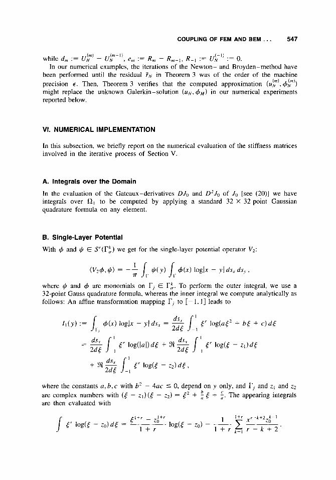
( m ) - (-1) while dm := UN In our numerical examples, the iterations of the Newton- and Broyden-method have

been performed until the residual FN in Theorem 3 was of the order of the machine precision E . Then, Theorem 3 verifies that the computed approximation ( u r ) , might replace the unknown Galerkin-solution (uN , q5,+,) in our numerical experiments reported below.

U f - I), e,,, := R,,, - R,,-l, R- I := UN := 0.

VI. NUMERICAL IMPLEMENTATION

In this subsection, we briefly report on the numerical evaluation of the stiffness matrices involved in the iterative process of Section V.

A. Integrals over the Domain

In the evaluation of the Gateaux-derivatives DJo and D'Jo of JO [see (20)] we have integrals over R l to be computed by applying a standard 32 X 32 point Gaussian quadrature formula on any element.

6. Single-Layer Potential

With 4 and (I, E Sr(r:) we get for the single-layer potential operator V2:

where (I, and 4 are monomials on Ti € T:. To perform the outer integral, we use a 32-point Gauss quadrature formula, whereas the inner integral we compute analytically as follows: An affine transformation mapping Tj to [- 1, I ] leads to

where the constants a , b, c with b2 - 4ac 5 0, depend on y only, and rj and 21 and 22

are complex numbers with (5 - z1)(5 - 22) = .f2 + ; ( + f . The appearing integrals are then evaluated with

h


C. Double-Layer Potential

For v E SP.q(R,) and $ E S'(ri) a typical term involving the double-layer potential operator is

where $ is a monomial on r, E ri. The outer integral we evaluate using a 32-point Gauss quadrature formula, whereas the inner integral we again compute analytically: With an affine transformation and related constants a . b , c , e , f satisfying b2 - 4ac 5 0,

To evaluate the appearing integrals we let R := a t 2 + 6 5 + c , A := 4ac - b2, and make use of

B c Xm-2 X m - I - - 1 F d t - - 1 R d 5

/ $ d t = (m - 1)A A A 1 1 f d 5 = - log(R) - -

2A 2A 1 $ = 2 arctan( 2A5 + B ) . dx A

D. Hypersingular Operator

For u, v E Sp.q(R;), we evaluate the hypersingular operator W2 with procedures of the single-layer potential operator (see [18]): ( u , W2v) = - ( V 2 z u , K V ) .

d d

VII. NUMERICAL RESULTS

For the computations we consider a couple of examples for the interface problem with R I being the square {(xI, x2) E R2: Ix, I < 1, i = 1,2}. In all examples we have

G ( r ) = /Ltp(t)dt =

F . u ] d x ,

so that 1 5 p ( r ) 5 3, 1 5 p ( r ) + r . p ' ( r ) 5 3, r > 0. With r 2 + r - log(1 + r ) , the functional Jo on H1(RI ) becomes

and with (15) we have P l u = -2Au - div(&) + u. In Tables 1-111 and Figs. 3, 4, and 5 , we present experimental rates of convergence for the L2-errors e := llul - K N IIL2(n,) in R I and E := 114 - 4t)llLqr) on r, where uI E H 1 ( R l ) and 4 = p(lVul I)% E H-1'2(I') solve the interface problem (15). In the sequel, mK denotes the number of iterations of the Newton-method, and NI and N2 denote the dimensions of S P . 4 and S', respectively.

( m )


TABLE I. Absolute errors in Example 1.

0.1 1358 0,03013 0,01181 0.00518

0,11358 0,01324 0,0028 15 0,000989

0,11358 0,01201 0,00422

4 17 48

112

4 17 48

112

4 17 48

u = 0.5: 1,5117 1,3554 1,1910 1,0433

1,5117 1,1679 0,9107 0,7141

1,5117 1,02482 0,70973

u = 0.25:

u = 0.1:

4 14 30 52

4 14 30 52

4 14 30

5 5 5

TABLE 11. Absolute errors in Example 2.

N , IIdJ - d J r K ) l l L ~ K ) N2 mK ( n l K ) IIU - U N llL2(Il,)

u = 0.25: 2,470 16 4 3,27856 4 2 0,07507 24 2,11075 16 5 0,005 175 84 0,7572 36 5 0,000695 217 0,2585 64 5

2,470 16 4 3,27856 4 2 0,03830 24 1,8602 1 16 5 0,01073 84 0,56459 36 5 0,OO 1690 217 0,170889 64 5

2,47016 4 3,27856 4 2 0,02678 24 1,75752 16 5 0,01667 84 0,47349 36 5 0,00 1246 217 0,130997 64 5

u = 0.2:

u = 0.171:

TABLE 111. Absolute errors in Example 3.

IIU - UjymK)IIL2(0,) Nl IIdJ - dJFK) I lL2W) N? mK

u = 0.25: 1,10564 4 3,27733 4 2 0,07415 24 3,41856 16 5 0,005366 84 2,80817 36 5 0,000620 217 2,23380 64 5

1,10564 4 3,27733 4 2 0,035443 24 3,26434 16 5 0,006374 84 2,50 149 36 5 0,000560 217 1,86517 64 5 0,000398 475 1,38318 100 5

u = 0.171:


e - - 1 1 4 0 z

10-22

10-3? -

10-4

-

4

E - u = 0.5 Il4llo - u = 0.5 h=O.l 0 u = 0.25 2.10-*- ~ 0 u = 0.25

1 o - ' p I I I I I I I I 10 I I I I I I I I

9 u = 0.25 0 u = 0.2

10-1-

1 0 - 2 p 1 I I I I I , I ,

fi U

FIG. 4. The relative error of Example 2.

3

FIG. 5 . The relative error of Example 3.


Example 1. Let the data functions be defined by

For the partition, fl:: = {Q', is a rectangle with the corners (1 - u'-', 1 - a'-' 1, ( 1 - u', 1 - a'-'), ( 1 - u'-', 1 - a'), (1 - a', 1 - u'), 1 5 i , j 5 n}, we use different constants u and appropriate polynomial degrees. See Fig. 1 for u = 7 .

The errors of the Galerkin procedure are shown in Table I and illustrated in Fig. 3. The exact solutions are given by

I

u ~ ( x ~ , x ~ ) = (2 - xI - x ~ ) ~ / ~ (X E fl,)

(x E a,). 1 2 U * ( X , , x* ) = - lo&; + x;)

Since u - rZ3, we have u E B$(Ql) (1/3 < p < 1 ) and E BF(I ' ) , (1 /3 < p < l ) , and get exponential convergence for IIu - u ~ I I ~ I ( R ~ ) and 114 - 4,,.,IIH IE(I-) [7], which is confirmed in this example. This is shown in Fig. 2 by the linear dependence of log & and m or 1% &) and a. Here llullo := IIUIIL'(R]) and Il4llo := ll4llL:(r).


16r2 - 32r' 32 16 9A

+ - A + 3 3(A-I + 8/3r) 9(A + 8/3rA2)? F(XI>X2) = - 2

+ A4 64r

9(A-I + 8/3r)? -

A := (2 - x: - , r := J.: + x i .

For this and the next example, we use the geometric mesh shown in Fig. 2. The corresponding errors of the Galerkin procedure are given in Table I1 and illustrated in Fig. 4. The exact solution is given by

U I ( X , , X 2 ) = (2 - x; - x;)4/3 (x E 01) 1 2 U2(XI, x2) = - lo& + x;) (x E a,).


Since u - r8‘3, we have u E @(al) (0 < p < 1) and E B $ ( T ) (0 < p < I ) , and we get exponentially fast convergence in the norms Ilu - U N I I H ~ ( ~ , ) and 114 - ~ M I I H - I / z ( ~ ) . This is confirmed in the numerical example, where we observe even exponential convergence of (4M) in t2(r) .


16r - 16r2 16 8 9A4 3A 3(A + 4 / 3 r ) 9(A + 4 /3r )2

8r2 9(A + 4 /3r )2 . A2

F ( X I , X 2 ) = - ~ + - +

+ + A2,

For this example, we also use the geometric mesh shown in Fig. 2. The corresponding errors of the Galerkin procedure are given in Table I11 and illustrated in Fig. 5. The exact solution is given by

Since u - r4I3, we have u E B$(fl , ) (0 < p < 1) and E B L ( T ) (1/6 < p < 1) that expect exponentially fast convergence in the energy norms. Numerically, we observe exponential convergence of Ilu - U N I I L ~ ~ , ) and 114 - ~ M I I L ~ ( ~ ) .

APPENDIX

Let .RI C R 2 be a bounded domain whose curvilinear boundary d Q I is a piecewise analytic curve T = U;=,T;, where Ti is an open arc connecting the vertices Ai and A ; + I ( A M + ~ = Al ) . Let a2 = R 2 \ f i 1 , we denote the internal angle at Ai by w ; . and assume 0 < w ; I 27r, 1 5 i I M. d /dn denotes the derivative with respect to the normal to r pointing from to a2.

Let f l I be a bounded open set in R 2 and let Hk(aI), k 2 0 integer, denote the usual Sobolev spaces (e.g. [ 191):

M -


where (Y = ( ( Y I , ( Y ~ ) , ai 2 0 integers, i = 1,2, IaI = ( Y I + ( ~ 2 , and

Hk-112 (r) is defined as the restriction of u E H k ( f l l ) to r for integer k 2 1 i.e.,

H k - 1 1 2 ( r ) = {U Ir: u E H k ( f l l ) }

with

and for k 5 0 by duality

Let r i ( x ) = d i s t ( x , A i ) , and let P = (P I , P 2 , . . . , P M ) be an M-tuple of real numbers 0 < Pi < 1. For any integer k 2 0, we shall write P + k = (PI + k , P2 + k , . . . , PM + k ) , and @ P + ~ ( X ) = nEIri ( x ) . As in [17], we define the weighted Sobolev space for integers k and 1, k 2 1 2 0, by

P, + k

H ; ' ( f l 1 ) = { u : u E H ' - ' ( f l , ) if 1 > 0, I I @ ' P + ~ a ~ - l D a ~ I ( L ~ ( ~ , ) < 03 for 1 5 la1 I k } ,

and the countably normed space for 1 2 0,

Bh(fl1) ={u: u E H : ' ( f l ~ ) t/ k 2 I, I l @ p + k - / D a ~ I I ~ * ( n l ) 5 Cdk-'(k - I)! for la1 = k = 1,l + 1 ,..., with C 2 I,d 2 1 independent of k } .

(r) [resp. Bk-112(I')] k , 1 integers, k I 1 2 1, is the trace The space H p (r) [resp. ~ k - I ~ ~ ( r ) ] space of ~2;"(n,) [resp. B ~ ( R ~ ) I , i.e., for any g E ~p

there exists G E H ; ' ( f l l ) [resp. Bh(fll)] such that G Ir = g, and ~ ~ g ~ ~ H ; - ~ ~ 2 . ~ - ~ ~ * (r) =

In the exterior domain f 1 2 , we incorporate the behavior of solutions at infinity. Let rr*(x) = mint], r i ( x ) ) for x E f12, then the weight function @ P + ~ ( x ) is modified by

k-112.1-112

k - 112. I- 112

infc ll.=g IIGIIHil(n,).

M

r = I k l The weighted Sobolev space, H,' ( f l 2 ) , k 2 1 2 2, is defined by

H2;"(f12) ={u: u E H;, , ( f l2) , D"u E L2( f12) for 2 5 I(YI < I , I l ~ p + i o t - ~ D a u I I ~ ? ( n ? ) < a, for 1 5 IaI 5 k } .

The definition of the space $(a2) is the same as B$(flI) .

The authors thank W. Thies for performing the numerical examples and the DFG for support. The work was partially supported by the DFG Forschergruppe "Zuverlassigkeit von Modellierung und Berechnung in der Angewandten Mechanik" at Hannover.

554 CARSTENSENANDSTEPHAN

References 1. J. Bielak and R. C. MacCamy, “An exterior interface problem in two-dimensional elastody-

namics,” Quart. Appl. Math. 41, 143 (1983). 2. M. Costabel, “Symmetry’s methods for the coupling of finite elements and boundary elements,”

in Boundary Elements IX, C. A. Brebia et al., Eds., 1, Springer-Verlag, Berlin, 1987, p. 41 1. 3. M. Costabel and E. P. Stephan, “Coupling of finite elements and boundary elements for inhomo-

geneous transmission problems in R3” in Mathematics of Finite Elements and Applications VI, J. R. Whiteman, Ed., Uxbridge 1987, Academic Press, London 1988, p. 289.

4. M. Costabel and E.P. Stephan, “Integral equations for transmission problems in linear elasticity,” J. Integral Equations Appl. 2, 21 1 (1990).

5. H. Han, “A new class of variational formulations for the coupling of finite and boundary element methods,” J . Comput. Math. 8, 223 (1990).

6. J. Johnson and J. C. Nedelec, “On the coupling of boundary integral and finite element methods,” Math. Comp. 35, 1063 ( 1 980).

7. N. Heuer, Die h-p Version bei der Randelementmethode, Ph.D. Thesis, UNI Hannover, 1992. 8. E. P. Stephan, “Coupling of finite elements and boundary elements for some nonlinear interface

problems,” Comp. Meth. Appl. Mech. Engineer. 101, 61 (1992). 9. C. Carstensen, “Interface problem in holonomic elastoplasticity,” Math. Meth. in the Appl. Sci.

16, 819 (1993). 10. C. Carstensen and E. P. Stephen. “Interface problem in elasto-viscoplasticity,” Quart. Appl.

Math., to appear. 1 1 . M. Costabel and E. P. Stephan, “Coupling of finite and boundary elements methods for an

elastoplastic interface problem,” SIAM J . Numer. Anal. 27, 12 12 (1990). 12. G. N. Gatica and G. C. Hsiao, “The coupling of boundary element and finite element methods for

a nonlinear exterior boundary value problem,” Zeitschrft fur Analysis und ihre Anwetidungen 8, 377 ( 1989).

13. J . NeEas and I. HlavaEak, Mathematical Theory of Elastic and Elasto-Plastic Bodies, Elsevier, Amsterdam, 198 1.

14. J. NeEas, Introduction to the Theory of Nonlinear Elliptic Equations, Wiley-Interscience, Chichester, 1986.

15. E. Zeidler, Nonlinear Functional Analysis and Its Applications IV, Springer- Verlag, New York, 1988.

16. C. Carstensen, S. A. Funken, and E. P. Stephan, “On the adaptive coupling of BEM and FEM in 2-d-elasticity;’ to appear.

17. B. Q. Guo and I. BabuSka, “The h-p version of the finite element method. Part 1 ,” Cornputat. Mech. 1, 21 (1986).

18. J. C. Nedelec, “Integral equations and non integrable kernels,” Integral Equations and Operator Theory 5, 563 (1982).

19. J . L. Lions and E. Magenes, Non-Homogeneous Boundary Value Problems and Applications I , Springer, Berlin, 1972.

Documents

Coupling of FEM and BEM for a nonlinear interface problem ...cc/cc_homepage/... · Coupling of FEM and BEM for a Nonlinear Interface Problem: The h-p Version ... Even in the case