FEDERAL SERVICE FOR HYDROMETEOROLOGY AND … · Semi-Lagrangian global model SLAV-2008 (jointly developed by the Hydrometcentre of Russia and the Russian Academy of Sciences), horizontal

1

RUSSIAN FEDERATION

FEDERAL SERVICE FOR HYDROMETEOROLOGY

AND ENVIRONMENTAL MONITORING OF THE RUSSIAN FEDERATION

(ROSHYDROMET)

ANNUAL JOINT WMO TECHNICAL PROGRESS REPORT ON THE GLOBAL DATA

PROCESSING AND FORECASTING SYSTEM (GDPFS) AND RELATED NUMERICAL

WEATHER PREDICTION RESEARCH ACTIVITIES FOR 2015

Country: Russian Federation Centre: WMC/RSMC: Moscow

09.06.2016

1. Summary of main highlights

Introduced into operation:

- New version of the Global spectral model Т339L31 (gaussian grid resolution is

approximately 32 km). Forecast lead time – up to 240 hours;

- Global system of ensemble forecast on the bases of two models T169L31 and SLAV-

2008 (14 members, lead time 10 days, breeding method);

- New versions of the regional mesoscale model COSMO-Ru with horizontal grid step 2,2

km, which includes continuous data assimilation cycles using “nudging” scheme for the

Central Federal district of Russia COSMO-Ru2CFO, Tatarstan (COSMO-Ru2VFO) and

the Northern Caucasia with adjacent areas offshore the Black Sea COSMO-Ru2SFO,

“inserted” into area of COSMO-Ru7 (grid 7х7 km) for the territories of East Europe and

European Russia, Urals and the western part of the West Siberia. Forecasts lead time - 42-

48 hours.

- Versions of the regional mesoscale model COSMO-Ru with horizontal grid step 13,2 km

for Europe and Northern part of Asia covering the entire territory of Russia, adjoining

areas onshore and offshore (COSMO-Ru13-ENA).

Introduced into quasi-operational trial regime:

- Global system of the seasonal forecasting with weekly discreetness and lead time up to 45

days. System is based on the global models of the Hydrometeorological Centre of Russia

and Russian Academy of Sciences (model SLAV-2008, 20 ensemble member) and model

of the Main Geophysical Observatory (model T42L14, 10 ensemble member);

- New version of the regional mesoscale model COSMO-Ru with horizontal grid

resolution 1.1 km for the resort Sochi area, including coastal zone and mountainous areas.

Model issuing forecasts with lead time up to 24 hours;

- New version of the Global semi-Lagrangean model SLAV 20 with grid step 20 km (in

operational trial);

- Experiments with the model of the deep ocean with inserted mixed layer for use in

seasonal forecasts of atmospheric conditions.

2

2. Equipment in Use

1) Autonomous server ASOOI – server1: 4 processors (4 x 8 cores) Intel Xeon E7-4830 2,13

GHz, memory 256 GB, discs 16 х 1 TB Ethernet 2 x 1 GBE, IPMI

2) Autonomous server ASOOI – server2: 4 processors (4 x 8 cores) Intel Xeon E7-4830 2,13

GHz, memory 256 GB, discs 16 х 1 TB Ethernet 2 x 1 GBE, IPMI

3) Cluster RSK: “Tornado” 96 nodes, Infiniband, each node: 2 processors (2 х 8 cores) Intel

Xeon E5-2690 2.9 GHz

4) Cluster ICEX: 30 nodes, Infiniband, each node: 2 processors (2 х 10 cores) Intel Xeon E5-

2670-v2 2.5 GHz

5) Total disc capacity for clusters: 210 Tb

3. Used Data and Products Coming from GST and other Communication Systems

Observational data (average number of telegrams per day)

WMC/RSMC Moscow

Code form Average number of

telegrams/day SYNOP+SHIP 128 000

TEMP 6 000

PILOT 1 650

AMDAR 78 000

AIREP 2 700

SATEM 17 000

SATOB 1 000 000

BUOY 33 000

BUFR-SYNOP 127 000

BUFR-TEMP 800

BUFR-AMDAR(ASDAR) 450 000

Additionally a heterogeneous satellite information is used - microwave AMSU-A and MHS,

radio-eclipsed COSMIC, GRAS and GRACE, scatterometric ASCAT and OSCAT, wind

(cloud movement) and humidity fields AMV-Geo, AMV-Polar and AMV-Leogeo. Total

amount of information received per day comprises 6,7 GB.

Products received at the WMC/RSMC Moscow:

ECMWF, Reading (analysis and forecasts of the general meteorological fields,

restricted list: GRIB 2.5 x2.5 and GRIB 0.5 x0.5 );

NMC Exeter (analysis and forecasts of meteorological fields of extended

nomenclature: GRIB1 2.5 x2.5 , GRIB2 1 x1 , forecasting maps for Europe: digital

facsimile);

RSMC Offenbach (forecasting maps: digital facsimile), Internet (FTP): GRIB1

0.25 x0.25 , GRIB2 20х20 km – product of the global DWD forecasting system with

horizontal resolution 20 km over the COSMO-Ru computational area necessaryID&BCfor the

operation of COSMO-Ru07 and COSMO-RuSib models- in framework of COSMO activities;

WMC Washington: Internetanalysis and forecasts of meteorological fields of extended

lists GRIB2 1 x1 , 0.5 x 0.5°);

3

RSMC Novosibirsk: site of the West Siberian Research Institute www.sibnigmi.ru: maps

in graphical format of all forecasting technologies of RSMC Novosibirsk (primarily, the

regional forecast using COSMO-RuSib;

RSMC Khabarovsk: products from the system of regional mesoscale forecasts for the

Far East and the seas of the Pacific basin.

4. Forecasting System

The global forecasting system of the WMC/RSMC Moscow is formed with the following

blocks:

А primary control and distribution of information from observations in specialized data

bases;

B systems of data assimilation and objective analysis;

C global atmospheric models;

D systems of modeling results interpretation;

The bounded areas forecasting system of WMC/RSMC Moscow includes the following

blocks:

А systems of receiving and control of initial information;

B atmospheric models for bounded areas;

C systems of automated visualization and preparation of data for distribution to users.

4.1 Time schedule and forecast range:

The basic initial times for forecasting system (global models SLAV-2008, T339L31 and

T169L31), regional model of Hydrometeorological Center of Russia MLp/s, are 00 and 12

UTC., The systems of Data assimilation are functioning for 00, 06, 12 18 UTC - 4 times a

day.

SLAV-2008 from initial data for 00 UTCforecasting period: 120 h (readiness time by 03.40

UTC), for initial data 12 UTC – forecasting period: 240 h (produced by 15.50 UTC).

Information is delivered to users with 6-hour time step. Technology includes additional

procedures for date assimilation of land-surface properties.

T339L31: for initial data 00 UTC forecasting period:78 h (readiness time – 5.30 UTC); for

initial data 12 UTC - forecasting period: 240 hours (readiness time 19 UTC). Information is

delivered to users with 6-h time step.

T169L31: same as for T339L31.

Regional forecasting technology COSMO-Ru07: initial data 00 and 12 UTC - forecasting

period 78 h, initial data 06 and 18 UTC – forecasting period 48 h with time step for products

delivered to users 1 hour for meteograms and 3 hours for GRIB generation (readiness time –

4.00, 10.00,16.00, 22.00 UTC). COSMO-Ru02 for Central (CFD), Southern Federal Districts

(SFD), and Tatarstan from initial data 00, 06, 12, 18 UTC – up to 48 hours with time step for

products presented to users 1 hour for meteograms and GRIB.

http://www.sibnigmi.ru/

4

Regional model of Hydrometeorological Center of Russia MLp/s for Europe:initial data 00 and

12 UTC - up to 48 h (readiness time – 4.00 UTC and 16.00 UTC). Information is provided in

graphical form with 1 hour time step.

Non-hydrostatic mesoscale model of Hydrometeorological Center of Russia with grid spatial

step 10х10 km for Moscow and Leningrad Districts and Belorus territory. Lead time is 48

hours. Output is produced with one hour time step. Readiness times are - 5.15 and 17.15 for

Moscow and 5.30 and 17.30 for St.-Petersburg and Minsk.

Short- and medium-range ensemble forecasting system is integrated once a day with initial

start time 12 UTC. Lead time – up to 240 hours with 6-hour time step.

Long-range forecasting systems – once a month starting one day before a coming month.

Hydrodynamic-statistical forecasts of the mean monthly anomalies of the surface temperatures

at the stations throughout the territory of the Former Soviet Union are produced at the end of

each month with zero lead time.

4.2. Medium-range forecasting systems (4 – 10 days)

4.2.1. Data assimilation, objective analysis and initialization

4.2.1.1. In operational mode:

The global system of data assimilation of the WMC/RSMC Moscow (Hydrometcentre of

Russia):

Cyclicity:

Cycle of the assimilation system – 4 times a day, observations for: 00, 06, 12, 18 UTC;

Objective analysis using the first approximation fields of RSMC Exeter and WMC

Washington – 2 times a day for 00, 12 UTC;

Method of analysis: two versions of technology:

a) 2-dimentional interpolation for 1-level characteristics and 3-dimentional optimal

interpolation for the fields within the bulk of atmosphere,

b) 3D-Var (under development)

Products – sea level pressure, surface air temperature, temperature of underlying

surface, surface air humidity and wind velocity, total octant cloudiness, snow cover

depth, sea surface temperature, geopotential heights at isobaric levels, wind velocity,

temperature and air humidity at 38 vertical isobaric levels (from 1075 to 0.5 hPa) at φ/λ

grid 0.5ºх0.5º;

The scheme of global cyclic data assimilation based on unified 3D-Var scheme

developed in the Hydrometeorological Centre of Russia using the global prognostic

atmospheric modal SLAV-2008 is testing in operational trial mode.

3D-Var system is using the following types of meteorological observations:

Traditional contact observations (surface, radiosounding, aircrafts), satellite observations:

microwave AMSU-A and MHS, radio-eclipsed COSMIC, GRAS and GRACE, scatterometric

ASCAT and OSCAT, wind (cloud movement) and humidity fields AMV-Geo, AMV-Polar

and AMV-Leogeo.

Objective analyses block uses the 6-hour NCEP (USA) forecasts as a first approximation

approach.

Horizontal resolution of objective analysis fields is 0.5ºх0.5º and 38 vertical levels (from 1075

to 0.5 hPa). Horizontal resolution of analysis increment fields in relation to forecast is 1.5°.

5

Initialization – non-linear, normal modes (for spectral T169L31 model) and digital filter (for

SLAV-2008 model).

Additionally, the system for generation of the initial fields of soil temperature and soil

humidity is included in the technology of SLAV-2008.

4.2.1.2 Research performed in this field:

Studies on applying of 3D-Var system for the global spectral atmospheric model T169L31 and

T339L31 are in progress.

Development of the local ensemble Kalman filter with ensemble transformation (LETKF)

assimilation scheme for the SLAV global semi-Lagrangian model are in progress. Currently,

the system assimilates observations from TEMP, SYNOP, SHIP, AIREP, SATOB and

demonstrates stable performance for the period of at least two months of cyclic assimilation

with 3-dimensional SLAV model. Works on introduction of AMV and ASCAT satellite

observation data are carried out. In particular, we have successfully tried to use non-diagonal

observation correlation matrix R for AMV data. The FGAT implementation in LETKF is

underway.

The system of the oceanographic data assimilation aimed at initializing the coupled ocean-

atmosphere model for seasonal forecasting has been developed. Data assimilation is carried out

on the basis of consequent scheme “analysis-forecast-analysis” using three-dimensional

assimilation at the step of analysis. The core of the scheme is represented by the new model of

the first approximation error fields based on the three-dimensional filters of auto-regression

and moving average. For obtaining the first approximation fields the oceanic global circulation

model is used. As initial information, the operative observations of the sea water temperature

and salinity coming from different observational platforms (drifting and anchored buoys,

vessel observations, data from ARGO buoys). The preliminary estimates show that the system

allows to simulate the structure of the main hydro-physical fields more accurately in

comparison with the climatic data.

4.2.2. Global Models

4.2.2.1. In operation mode:

Semi-Lagrangian global model SLAV-2008 (jointly developed by the Hydrometcentre

of Russia and the Russian Academy of Sciences), horizontal resolution 0.72ºx0.9º, 28

vertical levels. The maximum forecast range is 240 h. It produces a standard set of

prognostic products including total cloud amount and clouds of low and medium levels.

The Global spectral atmospheric model T339L31 with 339 spherical harmonics, grid

horizontal resolution of approximately 0.56º, 31 vertical levels. The maximum forecast

range is 240 h.

4.2.2.2. Research performed in this field:

A parameterization of the long-wave radiation RRTMG-LW v.4.85 was included in the

SLAV-20 model program complex.

The system of soil temperature and soil moisture initialization for multi-level

parameterization of the heat and moisture exchange processes in soil developed for the

climate model of the Institute of Numerical Mathematics of Russian Academy of

Sciences is under development. So far, SEKF soil moisture initialization is

implemented with the ISBA soil scheme used in SLAV2008 model.

6

Implementation of the hybrid vertical coordinate. Improvement of description of the

stratosphere: ozone advection and photochemistry.

Development of the new SLAV model version having about 10 km horizontal

resolution and about 100 vertical levels using the reduced lat-lon grid.

Development of version T339L63 with advanced block of solar radiation transfer

4.2.3. Operationally available medium-range Numerical Weather Prediction (NWP)

Products (Global modeling)

The output of the SLAV-2008, T339L31 and T169L31 models are accommodated at the

internal databases of Hydrometcenter of Russia at 2.5х2.5º and 1.25х1.25º grids (GRIB1). A

number of maps is transmitted in digital format to prognostic centers of Roshydromet and

Hydrometeorological Services of other countries via GTS. Forecasts in graphical format: maps

and meteograms are available on the website www.meteoinfo.ru. Forecasts for the Northern

and Southern Hemispheres with 6-h discontinuity intervals produce the following

characteristics: sea-level pressure, air temperature and humidity at 2 m, wind speed and

direction at 10 m, accumulated six-hour precipitation, geopotential heights, wind speed, air

temperature and humidity at standard isobaric surfaces, total low and medium level cloud

amount.

4.2.4. Applied operational techniques of NWP products (MOS, PPM, KF, Expert

Systems etc.), medium range forecast (72 – 240 h)


The system of statistical interpretation of the results of the medium range hydrodynamic

modeling (MOS) is used in Hydrometcenter of Russia. The automated system (on the basis of

the complex information coming from WMC Moscow, ECMWF Reading, NCEP Washington,

RSMC Exeter) provides the meteorological forecasts of extreme temperature, accumulated

semi-diurnal precipitation, precipitation probability, cloudiness – three times a day, with lead

time up to 7 days for 5000 cites over the globe including the settlements of the Russian

Federation.

On the basis of MOS system the forecasts of mean air temperature anomalies for the coming

10 days are calculated daily and send to the territorial Hydrometeorologival offices of

Roshydromet three times a month in the form of gif-charts and tables.

4.2.4.2. Research performing in this field:

The system of weather parameters forecasting using the MOS system of the

WMC/RSMC Moscow for bounded areas using mesoscale models is under development.

4.2.5. Ensemble Prediction System (EPS) (Number of members, initial state,

perturbation method, models used, perturbation of physical parameterizations, post-

processing: calculation of indices, clustering)


The ensemble prediction system (EPS) for short and medium ranges (12 – 240 h.) based on

T169L31 spectral global model and models T339L31 and SLAV-2008 model.

Ensemble is combined from 12 disturbed forecasts with T169L31 model and two undisturbed

forecasts with models T339L31 and SLAV-2008.

Characteristics of the system:

http://www.meteoinfo.ru/

7

Number of ensemble members: 14;

Number of models: 3;

Disturbance method: breeding using as a norm a total energy and regional rescaling;

Physical parameterizations are not disturbed.


Increasing a set of output products;

Development of postprocessing and verification methods;

Studies in the field of combining forecasts based on different models;

Development of statistical correction methods

Development of the ensemble prediction system based on LETKF (40 members) and

SLAV model.

4.2.5.3. Operationally available ensemble NWP products

The results of the EPS are placed to the operational database of the Hydrometcentre of

Russia; where they are available for Hydrometeorological Centre of Russia forecasters in the

form of spaghetti-charts, ensemble means and dispersion maps (a domestic visualization

system “Isograph” of the Hydrometcentre of Russia is recommended). Ensemble

meteogrammes for a number of settlements of Russia are produced. Since the beginning of

2015 meteograms are placed to the site of Hydrometeorological Centre of Russia and to the

site of SWFDP-CA project.

4.3 Short-range forecasting system (0-72 hours)

4.3.1. Data assimilation, objective analysis and initialization

4.3.1.1. In operational mode

The same as discussed in Section 4.2.1.1.

In COSMO-Ru technology a system of continuous assimilation of meteorological

information based on “nudging” scheme is implemented.


The same as in Section 4.2.1.2.

Additionally, a regional cyclic data assimilation with unified scheme is realized using

COSMO-Ru model.

Within the COSMO-Ru technology, the experiments on the assimilation of DMRs data

using the “nudging” scheme.

4.3.2. Models for short-range numerical forecasting

4.3.2.1. In operation

Non-hydrostatic model COSMO-Ru (developed within the consortium for mesoscale

modeling COSMO), version 4.12. Versions:

COSMO-RU7 - Horizontal resolution is 7x7 km, 40 vertical levels up to the surface of 100

hPa. The model produces forecasts for the territory of the East Europe, European Russia

and Urals.

8

COSMO-Ru2 – grid 2.2x2.2 km for the Central Federal District of Russia (COSMO-

Ru2CFO), Tatarstan (COSMO-Ru2VFO) and Northern Caucasia (COSMO-Ru2SFO)

inserted into COSMO-Ru7.

COSMO-Ru13-ENA (grid 13.2х13.2 km). Area of integration covers Europe, Northern

Asia including the entire territory of Russia, adjacent areas onshore and offshore.

Regional non-hydrostatic model for the European region (area of forecast 137x209 grid

points of the equal Cartesian grid (horizontal step 50 km, 30σ-levels). It produces

information on expected weather, in particular precipitation and surface characteristics,

the discreteness of output products with 1 hour time step. The adapted versions of the

regional model of the Hydrometcentre of Russia have been put into operation at RSMC

Novosibirsk and RSMC Khabarovsk. Two versions of the model were implemented

operationally for the Far East and North Caucasus regions with horizontal resolution 25

km.

Mesoscale non-hydrostatic model (15 levels in the atmosphere) for the Moscow and

Saint-Petersburg with 10 km resolution.

4.3.2.2. Research performed in this field

The priority projects studies within the framework of the COSMO Working groups’

activities include: development and testing of the enhanced scheme of snow cover,

analysis of the specifics of the radiation block operation, development of the scheme

describing the turbulent fluxes in the lower boundary layer, development of verification

system, and enhanced algorithms of the more accurate initial information preparation

based on the observational data SYNOP. These include also the development of the

forms of presentation of the forecast results to users, and monitoring and studies of

success of the near surface weather parameters forecasts using COSMO-RU model

(surface air temperature, precipitation, wind speed).

Development of the COSMO-RuENA (13х13 km) version for the entire territory of

Europe, northern Asia and adjusting seas.

Research of the COSMO-Ru1 version (1x1 km)

- Development of verification systems for mesoscale NWP.

4.3.3. Available operational products of numerical weather forecasts (modeling for

bounded territories)

4.3.3.1 Products of the mesoscale modeling system COSMO-Ru:

Forecasts of the sea level pressure, 3-h accumulated precipitation, surface temperature

and wind, cloudiness, 500 hPa height – in the form of GRADS maps. Information in the form

of meteorological cables for more than 100 points within the European part of Russia, with

time resolution of 1 h in text and graphical formats: forecasts of sea level pressure,

accumulated precipitation considering precipitation forms, temperature and wind profiles from

the ground surface up to 500 hPa, cloudiness within the different layers (Information is

provided to users in graphical formats via e-mail and distribution at the ftp server.

Wide range of meteorological characteristics at p, z and σ-levels in GRIB formats are

provided to users upon request.

4.3.3.2 Products of the versions of regional model of the Hydrometeorological Centre

of Russia (50x50 and 25x25 km) for different regions::

The entire territory of Russia and Europe, eastern part of Atlantic ocean, Northern

Caucasia, Black sea, and Far East with adjacent seas.

Products:

9

Sea level pressure fields, surface temperature and 1-hour precipitation intensity

(detailed once an hour);

fields of geopotential heigh, wind components, temperature and relative

humiditystandard isobaric surfaces (detailed each 3 hours;

fields of the semi- and daily accumulated precipitation: continuous, convective and

total (lead time 12, 24, 36, 48 hours).

Information is provided to users via data bases and in graphical formats through distribution

via e-mail and posting on the site www.meteoinfo.ru (forecasts of the sea level pressure, 1 and 3-

hour accumulated precipitation).

4.3.3.3 Production of the mesoscale non-hydrostatic model of the Hydrometeorological

Centre of Russia (10х10 km):

Forecasts of surface air temperature and wind are provided with 1 h time step for the

Moscow and St.-Petersburg regions. Results are placed to the WMC/RSMC Moscow

databases. Data are transmitted via FTP.

4.3.4. Operational techniques for application of NWP products MOS, PPM, KF,

Expert Systems, etc.), short range forecasts (0 – 72 h)


The system of statistical interpretation of the hydrodynamic modeling results (MOS

system) is used, (see Section 4.2.4.1).

Interpretation system based on statistical correction of the global modeling results:

extreme temperatures and values of T2m temperature for the fixed time of measurements,

wind speed and direction, accumulated precipitation for meteorological stations of Russia.

A system for physical-statistical interpretation based on the regional numerical model

results producing short-range forecasts of hazardous weather phenomena (thunderstorms,

showers, hail, strong squalls) with the lead time up to 36 h is in operation.

Post-processing for aviation:

a) On the basis of output of the COSMO-Ru model with horizontal resolution 7 and 2.2

km: a set of meteorological characteristics and maps (height of the upper and lower boundaries

of convective and stratified clouds, levels of icing, turbulence intensity in the lower layer, zero

isotherm heigh, cloud amount, etc.) for the airports in the European part of Russia with lead

time up to 48 hours.

b) On the basis of the SLAV-2008 model output data: characteristics of convective

clouds (height of the upper and lower confines), levels and values of the maximum wind

speed, height of dynamic tropopause, heights of the boundaries of icing and turbulence zones,

and complex indicators (frontier parameter) with lead time up to 36 hours.

4.3.4.2. Research in this field

Improvement of all systems mentioned in Section 4.3.4.1.

4.3.5 Ensemble Prediction System (EPS) (Number of members, initial state,

perturbation method, models and number of models used, perturbation of physical

parameterizations, post-processing: calculation of indices, clustering)



10

Same as shown in Section 4.2.5.1.

Currently no mesoscale ensemble forecasts are issued.

4.3.5.2. Research performed in this field

Same as shown in Section 4.2.5.2

Additionally, research in model-related forecast uncertainty resulted from imperfection of the

atmospheric model and its influence on forecast skill was conducted.

Comparison of the ensemble forecast results obtained using different schemes within the

framework of FROST-2014 project.

4.3.5.3. Operationally available ensemble NWP products

Same as discussed in Section 4.2.5.3

Since June 2014 operative integration of mesoscale ensemble forecasts for Sochi region

was completed.

4.4 Nowcasting and Very Short-range Forecasting Systems (0-6 hrs)

4.4.1 Schemes of nowcasting

4.4.1.1 In operation

No nowcasting schemes are in use in WMC/RSMS Moscow in operational mode.

4.4.1.2 Research performed in this field

The nowcasting method based on the forecasts of the COSMO-RU and WRF-ARW models is

under development. Method utilizes information from geostationary satellites and radars.

Research within the framework of the international operative-demonstrational WMO project

FROST-2014 for meteorological support of Olympic Games Sochi 2014.

Debugging works on adaptation of nowcasting statistical complex for precipitation fields based

on the consequent fields of precipitation intensity obtained with interpretation of reflectivity

from Doppler radars deployed over the territory 0f the Central Federal District (CFD) and

operated by the Central Aerologic Observatory (CAO) of Roshydromet.

First results of ensemble forecasts with several hours lead time based on the initial fields of

radar precipitation separated with 10 minutes time intervals are obtained.

11

4.4.2 Models used in very Short-range Forecasting Systems.


Not used.


Adaptation of the non-hydrostatic model COSMO-Ru (developed within the consortium for

mesoscale modeling COSMO) for nowcasting in configuration COSMO-Ru2.

COSMO-Ru2 – grid 2.2x2.2 km in the versions for the Central Federal District of Russia

(COSMO-Ru2CFO), Tatarstan (COSMO-Ru2VFO) and Northern Caucasia (COSMO-

Ru2SFO) inserted into COSMO-Ru7

4.5. Specialized numerical predictions (sea waves, storm surge, sea ice, marine

pollution transport and weathering, tropical cyclones, air pollution transport and

dispersion of pollutants, solar ultraviolet (UV) radiation, air quality forecasting, smoke,

sand and dust.

4.5.1 Assimilation of specific data, analysis and initialization


The system of oceanographic data assimilation was implemented for initialization in the

coupled ocean-atmospheric model for seasonal forecasting. The core of the system is the new

model of the first approximation errors field based on the tree-dimensional autoregression

filters and moving average. For obtaining the first approximation fields, the general circulation

oceanic model is used. Preliminary results demonstrate that the system produces the structure

of the hydrophysical fields more accurately than the climatic models.


Works on transfer of the oceanographic date assimilation system to new model of ocranic

general circulation NEMO (The Nucleus for European Modelling of the Ocean) using de-parallel

program code and three-pole computational grid allowing capability to conduct global assimilation

including Arctic basin..

4.5.2 Specialized models


А) Sea wave forecasting:

1) Forecasts based on the spectral-parametric model of wind waves are issued in the

operational mode. The solution for the model is based on the division of the spectrum into 2

components: wind waves and swell waves. For wave forecast the objective analysis data and

the output of the global spectral T169L31 atmosphere model of the Hydrometcentre of Russia

are used for diagnosis and wind velocity forecast on1.25 x1.25 grid.

2) Operational forecasts of the wind wave characteristics (high of significant waves,

average direction of propagation, aver4age length, average period, high and direction of

propagation of wind waves high and direction of propagation of swell waves) are given using

the spectral model WaveWatch III v.3.14. Forecasts are given for a five day period using

meteorological numerical forecast information (model SLAV and GFS system) for the World

ocean (grid 0.5°x0.5°) and for distinct seas: Baltic sea (grid 1.2'×1.2', ~2 km), Caspian sea

12

(grid 3.6'×3.6', ~6 km), Barewnts sea (grid 0.25 ×0.1 , ~10 km), and White sea (grid 3.0'×1.2',

~2 km). Forecasting results are available at website http://hmc.meteorf.ru/sea/.

B) Forecast of sea level variations and sea current velocity :

The system of short-range forecasting (up to 48 hours) of the sea level variations and current

velocity for the Barents and White seas based on calculations of the three-dimensional

hydrodynamic model with free surface considering tidal flows with 4-km grid step. As input

meteorological information, the atmospheric pressure forecasts from the regional atmospheric

model of the Hydrometeorological Centre of Russia Mlσ are used. Results of forecasts are

placed at the website http://hmc.meteorf.ru/sea/index.html.

C) Long-Range forecasting of sea ice in non-Arctic seas of Russia:

Long-range forecasts (with lead time of several months) of sea ice cover are produced

regularly. The forecasts include the first date of ice occurrence in the ports, maximum sea

icing, maximum thickness of fast ice, dates of ablution of ports from ice, duration of ice

period. Forecasts are based on the notion of the cyclist character of the hydrometeorological

elements variability and influence of the thermobaric fields during the period, preceding the

icing. As the predictors for forecasts a correlation of the ice parameters and atmospheric

pressure and temperature during preceding period.

D) In Hydrologic department of WMC Moscow the models Cosmo-Ru 13 (for

European Russia – 7 km), and regional model of Hydrometcentre of Russia (resolution 25 km),

as well as forecasts of NCEP-NCAR and ECMWF are used to predict the river water yield are

used. During the spring freshets the river ice model developed in Hydrometcentre of Russia is

used.


A new version of the storm surges forecasting model using as the initial data the output of the

regional hydrodynamic model of Hydrometeocenter of Russia Mlp/MlϬ .

To determine the forecasts quality dependence of the sources of meteorological information,

verification of wind wave forecasts is conducted along the entire World ocean.

4.6 Extended range forecasts (10 to 30 days), Models, Ensembles, Methodology

The global general circulation model SLAV-2008 currently represents a core of probabilistic

numerical long-range forecast of meteorological conditions. Jointly with Main Geophysical

Observatory of Roshydromet named after Voeykov (MGO) a pilot technology of weekly

detailed scheme of multi model forecast with lead time up to 1.5 months is implemented in

WMS Moscow.

4.6.1 Models used

Model SLAV-2008 is a semi-Lagrange finite-different global model of atmospheric general

circulation developed in the Institute of Numerical Mathematics of Russian Academy of

Sciences and Hydrometeorologichescal Centre of Russia. Semi-Lagrange method of

calculation of advection allows to use in the model time step several times larger than the step

envisaged by the CFL number. Specific of block of solution of atmospheric dynamics

equations uses fourth-order finite differences at the unstaggered grid to approximate non-

advective terms of equations and uses the vertical component of absolute vorticity as

prognostic variable. Block of solutions of atmospheric dynamics equations is described in

details in [27-29].

http://hmc.meteorf.ru/sea/index.html

13

Model includes a set of parameterization of sub-grid scale processes (short- and long-wave

radiation, deep and shallow convection, planetary bounder layer, gravitational waves drag,

parameterization of heat and moisture exchange with underlying surface) developed in Meteo

France and meteorological services of RC-LACE consortium (Limited Area modeling for

Central Europe) (http://www.rclace.eu) for French global operational model ARPEGE and

regional model of international consortium ALADIN/ALARO. Model generates 20 ensemble

members using breeding technique of escalating growing modes. Hindcasts initial data are

taken from ERA Interim reanalysis. The boundary conditions are determined from initial

anomalies of SST during the entire period of forecast.

The MGO forecasting system is based on calculation of evolution of atmospheric conditions

during the period of forecast using the physically complete global spectral model of general

circulation T63L15 (horizontal resolution 1.9 1.9 , 25 vertical layers, time step ~10 minutes).

Period of forecast is 127 days. The previously developed block of physical processes

parameterizations is used in the new version of the model excluding calculation of gravity wave

resistance and horizontal diffusion, which depend on model resolution and require special

adjustment. As a result of model validation some coefficients and conditions used in the

schemes of physical processes parameterizations were changed. These changes allowed to

minimize the systematic errors.

Boundary conditions (SST) are consider the conservative initial temperature anomalies during

the whole period of integration. In comparison with the earlier version of the model the

distribution of sea ice is changed. Instead of climatic distribution the initial anomalies of sea

ice distribution are used, which kept conservative during 14 days period with further relaxation

toads climatic distribution. Considering the observational data during resent 20 years (1992-

2011) the climatic fields of SST and sea ice characteristics were determined more precisely. To

determine probabilistic forecasting distribution the calculation of ensemble forecast (10

ensemble members) are used.


- Numerical model SLAV-2008 is used in operational regime. Current and retrospective

forecasts are produced every week for 63 days period, and two times a month for 135 days.

Model post processing generates 68 fields of atmospheric and surface meteorological

characteristics as an output at the global latitude-longitude grid 1.5° х 1.5 °.

- Forecasts produced in MGO with the T63L25 model are transmitted operationally to

Hydrometcentre of Russia in jointly agreed format. According conditions of operational

testing, the following time averaging intervals are chose: 1-7 days (1 week); 8-14 days (2

weeks); 15-21 days (3 weeks); 22-28 days (4 weeks); 1-30 days (1 month); 15-45 days (2-nd

month). It is possible to scrutinize the results of forecast with daily discreetness, which let

producing forecasts of variable time of averaging. Such flexibility allows to change time

windows of forecast and better estimate the quality of forecast

-Statistical interpretation block implemented at NEACC server includes procedures allowing

to realize operatively on the basis on predicted by SLAV-2008 and MGO models global

surface air temperature, the temperature at the stations. Method of by linear interpolation is

used as the basic method of processing of initial information. Resulting outcome of these

procedures is predicted surface air temperature at 70 stations of the FSU.


A statistical structure of daily climatic archives of air temperature at 2 meters and precipitation

necessary for obtaining normalized forecasting anomalies is analyzed.

14

Possibilities of using teleconnection between surface air temperature and meteorological field

characteristic with large-scale patterns of atmospheric circulation and thermal conditions at the

underlying surface are considered. It is supposed to estimate additional effects of using

teleconnections based on the estimates of the quality of forecasting products.

On the basis of the methods of decision making theory, possibilities of development of

methods of selection such products, which could be optimal to some extent or prediction of

certain specific meteorological variables in certain geographic conditions are explored.

4.6.2 Operationally available ensemble prediction systems products for 10-30 days:

Forecasts of mean monthly temperature fields are regularly placed on the web-site of the

Hydrometcentre of Russia http://www.meteoinfo.ru. Forecasts of air temperature fields near land

surface and at the standard isobaric surfaces 500 and 850 hPa, and also those of surface air

temperature values for 75 settlements of the former USSR are available to users upon request.

Forecasts of the main meteorological fields, specifically H500, T850, sea level pressure and

precipitation with week lead time are placed weekly at the site of NEACC http://seakc.meteoinfo.ru/

4.7 Long-range forecasts (30 days - 2 years), Models, Ensembles, Methodology

4.7.1. In operation:

A technology of global ensemble forecasts with 4 months lead time is realized in

Hydrometeorological Centre of Russia. It is based on using models developed in

Hydrometeorological Centre of Russia (SLAV-2008) and MGO (T42L14). Maps of the main

meteorological fields H500, T850, sea level pressure, surface air temperature, and precipitation

are produced with one month and seasonal lead time are produced and placed on NEACC’s

site http://seakc.meteoinfo.ru/ every month.

Forecasts of the monthly average temperature and precipitation for the FSU territory with lead

time up to 6 months for cold and warm periods of the year based on the complex research and

development of the scientific institutes of the Russian Hydrometeorological Service

(Hydrometeorological Centre of Russia (HMC), Voeykov Main Geophysical Observatory

(MGO), Arctic and Antarctic Research Institute, and Far East Hydromet Institute) are available

at the site of Hydrometcentre of Russia http://www.meteoinfo.ru.

Within the framework of international cooperation and participation of Hydrometcentre of

Russia in APCC project (Pusan, Republic of Korea) global ensemble forecast for 4 months

period are produced monthly with one month lead time.

The forecasts for the nearest three months are produced monthly and forwarded to the Asian-

Pacific Climate Centre (APCC) (Busan, Republic of Korea) as a contribution to the multi-

model ensemble seasonal forecast within the framework of the international project APCN

(Asia-Pacific Climate Network) on the long-range forecasting (Seoul, Republic of Korea).

4.7.2. Research performed in this field:

A continuous work on improving the SLAV model is carried out. It is oriented specifically on

improvement of blocks of parameterization of short- and long-wave radiation, cloudiness,

boundary layer, soil ice, and ozone layer.

Possibilities of adaptation of different statistical methods of regional elaboration are explored

(e.g. regression method, , probabilistic approach, etc.) aimed to improve global forecast of

meteorological fields.


http://seakc.meteoinfo.ru/

http://seakc.meteoinfo.ru/


15

Using the global semi-Lagrangean model SLAV, the studies of regional predictability of low-

frequency variability and related regimes of atmospheric circulation at monthly and seasonal

time intervals in the Northern Hemisphere are conducted.

Technical efforts on presentation of historical forecasts in compliance with protocols of

international projects CHFP и S2S are carried out.

4.7.3. Operationally available products:

Results of the seasonal forecasts of the WMC Moscow using the corresponding hindcast

verifications for primary seasons of the year are presented on the site

http://wmc.meteoinfo.ru/season, http://wmc.meteoinfo.ru/ПЛАВ.

Every month the results of 3-month seasonal forecasts with one month lead time and the

corresponding hindcast seasonal forecasts data of the WMC Moscow are forwarded to the

Asian Pacific Climate Centre (APCC) (Busan, Republic of Korea) as an input to the multi-

model ensemble seasonal forecast in the framework of the international APCN (Asia-Pacific

Climate Network) project on long-range forecasting (LRF). Once a month the seasonal

forecasts of the SLAV model with one month lead time are forwarded to the WMO Leading

Centre for Multi-model Long-range forecasting in Seoul, Republic of Korea. The list of

transmitted forecasting characteristics include monthly averaged and 3-month global fields of

geopotential height of the 500 hPa surface, temperature at 850 hPa, sea level pressure, bottom

level air temperature and accumulated precipitation for individual ensemble members.

Forecasts of monthly averaged air temperature and precipitation for the FSU territory with 6-

month lead time for cold and warm periods of the year based on the complex research and

development of the scientific institutes of the Russian Hydrometeorological Service

(Hydrometeorological Centre of Russia (HMC), Voeikov Main Geophysical Observatory

(MGO), Arctic and Antarctic Research Institute, and Far East Hydromet Institute) are

presented on the site http://meteoinfo.ru/veget-period-2014

Forecasts of air temperature and precipitation for one month with zero lead time for the FSU

territory based on the NWP (spectral HMC model, spectral MGO model) and synoptic-

statistical forecasts are placed on site http://meteoinfo.ru/1month-forc

http://wmc.meteoinfo.ru/season

http://wmc.meteoinfo.ru/ПЛАВ

http://meteoinfo.ru/veget-period-2014

http://meteoinfo.ru/1month-forc

16

5. Forecast results verification

5.1. Year average estimates

5.1. The global semi-Lagrangian model of the Hydrometcentre of Russia and the Institute

for the Computational Mathematics of the Russian Academy of Sciences (SLAV-2008) for

00 and 12 UTC initial data is in operational use since 2010 on the grid 1.5x1.5° updated in

2012 is available on the site (http://www.wmo.int/pages/prog/www/DPFS/Manual_GDPFS.html).

5.1.1. SLAV-2008, Northern hemisphere (20N-90N)

5.1.1.1 SLAV-2008, Northern hemisphere. Sea level pressure

Lead time ME (hPa) RMSE (hPa) KA S1

(hours) 00 UTC 12 UTC 00 UTC 12 UTC 00 UTC 12 UTC 00 UTC 12 UTC

24 -0,123 -0,061 1,610 1,563 0,976 0,977 0,324 0,325

48 -0,109 -0,113 2,364 2,308 0,948 0,949 0,398 0,399

72 -0,190 -0,199 3,258 3,191 0,901 0,904 0,475 0,476

96 -0,226 -0,210 4,270 4,173 0,832 0,837 0,552 0,554

120 -0,227 -0,219 5,326 5,234 0,742 0,746 0,624 0,627

144 -0,185 6,273 0,640 0,691

168 -0,218 7,177 0,535 0,742

192 -0,245 7,919 0,436 0,782

216 -0,263 8,577 0,347 0,813

240 -0,323 9,101 0,278 0,835

5.1.1.2. SLAV-2008, Northern hemisphere, H 850 hPa

Lead time ME (m) RMSE (m) KA S1


24 0,220 -0,225 11,253 11,766 0,981 0,979 0,292 0,296

48 0,558 -0,546 16,764 17,210 0,959 0,955 0,368 0,371

72 0,025 -1,183 23,474 23,754 0,919 0,916 0,447 0,449

96 -0,108 -1,150 31,274 31,123 0,857 0,857 0,526 0,527

120 0,054 -1,143 39,538 39,356 0,773 0,772 0,600 0,601

144 -0,728 47,496 0,671 0,667

168 -0,887 54,560 0,570 0,718

192 -1,040 60,499 0,472 0,758

216 -1,059 65,790 0,384 0,791

240 -1,414 70,127 0,311 0,816

http://www.wmo.int/pages/prog/www/DPFS/Manual_GDPFS.html

17

5.1.1.3. SLAV-2008, Northern hemisphere (20N-90N), H 500



24 -2,047 -2,382 11,818 11,992 0,992 0,991 0,186 0,185

48 -0,446 -1,536 19,575 19,773 0,977 0,976 0,264 0,263

72 -0,203 -1,451 29,619 29,565 0,945 0,945 0,345 0,344

96 0,348 -0,777 41,508 40,929 0,892 0,893 0,425 0,422

120 1,190 -0,192 54,188 53,673 0,814 0,815 0,499 0,497

144 0,741 66,528 0,717 0,564

168 1,126 77,907 0,614 0,618

192 1,499 88,011 0,510 0,662

216 1,970 96,218 0,418 0,696

240 2,150 102,864 0,340 0,721

5.1.1.4. SLAV-2008, Northern hemisphere (20N-90N) H 250



24 -0,611 -0,253 16,429 16,141 0,992 0,992 0,162 0,162

48 3,854 3,427 27,509 27,391 0,977 0,976 0,232 0,232

72 6,686 6,227 41,155 41,214 0,947 0,946 0,303 0,304

96 9,443 9,077 57,904 57,209 0,894 0,896 0,376 0,374

120 12,375 11,838 75,631 74,875 0,820 0,822 0,445 0,444

144 14,488 92,541 0,728 0,506

168 16,366 108,380 0,628 0,557

192 17,900 122,820 0,526 0,601

216 19,306 134,664 0,433 0,634

240 20,327 144,344 0,351 0,660

5.1.1.5. SLAV-2008, Northern hemisphere (20N-90N)

Air temperature at 850 hPa

Lead time ME (K) RMSE (K) KA

(hours) 00 UTC 12 UTC 00 UTC 12 UTC 00 UTC 12 UTC

24 0,066 -0,045 1,643 1,770 0,911 0,893

48 0,114 -0,019 1,949 2,058 0,877 0,860

72 0,144 -0,001 2,296 2,387 0,833 0,817

96 0,181 0,025 2,712 2,781 0,772 0,759

120 0,218 0,046 3,167 3,224 0,694 0,683

144 0,069 3,688 0,594

168 0,086 4,126 0,501

192 0,100 4,513 0,409

216 0,123 4,806 0,335

240 0,148 5,049 0,271

18





24 -0,189 -0,136 0,949 0,928 0,965 0,965

48 -0,081 -0,031 1,330 1,313 0,929 0,929

72 -0,019 0,031 1,777 1,769 0,875 0,874

96 0,039 0,090 2,272 2,247 0,799 0,801

120 0,100 0,151 2,764 2,737 0,705 0,708

144 0,203 3,202 0,605

168 0,256 3,605 0,505

192 0,307 3,962 0,408

216 0,351 4,224 0,330

240 0,394 4,442 0,264





24 0,480 0,482 1,400 1,368 0,930 0,932

48 0,606 0,609 1,862 1,827 0,868 0,870

72 0,726 0,746 2,280 2,254 0,794 0,795

96 0,811 0,837 2,682 2,651 0,704 0,705

120 0,890 0,922 3,048 3,018 0,609 0,608

144 0,975 3,320 0,517

168 1,020 3,563 0,438

192 1,038 3,773 0,364

216 1,054 3,935 0,305

240 1,070 4,061 0,256


Wind speed at 850 hPa

Lead time MEAN SPEED ERROR

(m/s) RMSEV(m/s)

(hours) 00 UTC 12 UTC 00 UTC 12 UTC

24 -0,367 -0,368 3,329 3,283

48 -0,442 -0,451 4,270 4,210

72 -0,517 -0,526 5,305 5,233

96 -0,576 -0,579 6,387 6,302

120 -0,608 -0,613 7,434 7,350

144 -0,626 8,280

168 -0,627 9,009

192 -0,622 9,566

216 -0,627 10,038

240 -0,614 10,405

19


Wind speed at 500 hPa


(m/s) RMSEV(m/s)


24 -0,274 -0,281 3,903 3,892

48 -0,397 -0,421 5,431 5,392

72 -0,464 -0,501 7,087 7,017

96 -0,512 -0,555 8,798 8,688

120 -0,546 -0,582 10,458 10,359

144 -0,591 11,904

168 -0,603 13,166

192 -0,621 14,216

216 -0,628 15,043

240 -0,649 15,663


Wend sped 250 hPa


(m/s) RMSEV(m/s)


24 -0,708 -0,659 5,591 5,515

48 -0,866 -0,865 7,868 7,805

72 -1,025 -1,024 10,248 10,221

96 -1,178 -1,188 12,818 12,701

120 -1,254 -1,267 15,372 15,225

144 -1,347 17,513

168 -1,402 19,433

192 -1,492 21,079

216 -1,577 22,436

240 -1,666 23,439

5.1.2. SLAV-2008, Tropics (20N-20S)

5.1.2.1. SLAV-2008, Tropics (20N-20S). Sea level pressure

Lead time RMSE (hPa) KA S1


24 1,028 1,028 0,780 0,773 0,452 0,466

48 1,396 1,354 0,652 0,661 0,484 0,501

72 1,689 1,627 0,564 0,585 0,513 0,529

96 1,820 1,717 0,517 0,560 0,533 0,547

120 1,951 1,864 0,471 0,512 0,550 0,564

144 1,972 0,457 0,580

168 2,093 0,397 0,595

192 2,184 0,348 0,607

216 2,266 0,297 0,617

240 2,335 0,250 0,625

20

5.1.2.2. SLAV-2008, Tropics (20N-20S), H 850 hPa

Lead time RMSE (m) KA S1


24 8,428 8,685 0,774 0,755 0,534 0,538

48 11,250 11,410 0,656 0,627 0,574 0,581

72 13,534 13,564 0,566 0,540 0,617 0,620

96 14,335 14,076 0,526 0,513 0,643 0,646

120 15,259 15,166 0,479 0,459 0,667 0,670

144 15,830 0,407 0,692

168 16,662 0,347 0,712

192 17,080 0,312 0,729

216 17,612 0,264 0,740

240 18,071 0,221 0,752




24 8,077 8,116 0,863 0,871 0,486 0,484

48 9,497 9,728 0,798 0,796 0,536 0,534

72 10,894 11,212 0,735 0,726 0,584 0,579

96 11,514 11,730 0,702 0,692 0,619 0,616

120 12,555 12,837 0,644 0,632 0,655 0,652

144 13,972 0,561 0,685

168 15,217 0,480 0,714

192 15,964 0,422 0,739

216 16,906 0,352 0,761

240 17,662 0,291 0,777




24 11,206 10,945 0,895 0,898 0,399 0,402

48 13,673 13,285 0,836 0,844 0,451 0,454

72 16,171 15,456 0,772 0,788 0,492 0,497

96 18,715 17,725 0,702 0,723 0,527 0,533

120 21,370 20,139 0,619 0,644 0,562 0,567

144 22,627 0,556 0,600

168 24,804 0,471 0,629

192 26,732 0,395 0,653

216 28,458 0,325 0,674

240 30,225 0,255 0,694

21

5.1.2.5. SLAV-2008, Tropics (20N-20S), temperature at 850 hPa

Lead time RMSE (K) KA


24 1,308 1,325 0,576 0,583

48 1,419 1,435 0,516 0,525

72 1,519 1,539 0,466 0,475

96 1,611 1,647 0,419 0,421

120 1,700 1,747 0,374 0,372

144 1,842 0,322

168 1,942 0,267

192 2,036 0,214

216 2,109 0,171

240 2,166 0,135




24 0,739 0,731 0,795 0,789

48 0,889 0,891 0,698 0,687

72 0,994 0,988 0,622 0,619

96 1,092 1,073 0,548 0,551

120 1,177 1,154 0,482 0,484

144 1,229 0,419

168 1,304 0,354

192 1,367 0,293

216 1,415 0,246

240 1,466 0,204




24 0,918 0,875 0,670 0,693

48 1,170 1,120 0,505 0,526

72 1,335 1,274 0,375 0,401

96 1,448 1,380 0,284 0,313

120 1,524 1,454 0,217 0,247

144 1,503 0,196

168 1,528 0,156

192 1,544 0,125

216 1,557 0,101

240 1,566 0,081

22

5.1.2.8 SLAV-2008, Tropics (20N-20S), Wind speed at 850 hPa


(m/s) RMSEV(m/s)


24 -0,466 -0,477 2,942 2,860

48 -0,723 -0,722 3,587 3,502

72 -0,895 -0,912 4,092 4,031

96 -1,064 -1,056 4,547 4,486

120 -1,134 -1,123 4,906 4,833

144 -1,151 5,118

168 -1,232 5,411

192 -1,266 5,628

216 -1,337 5,819

240 -1,355 5,953

5.1.2.9 SLAV-2008, Tropics (20N-20S), Wind speed at 500 hPa


(m/s) RMSEV(m/s)


24 -0,316 -0,313 2,994 3,005

48 -0,383 -0,390 3,912 3,935

72 -0,372 -0,374 4,653 4,669

96 -0,385 -0,388 5,286 5,281

120 -0,419 -0,431 5,823 5,800

144 -0,476 6,262

168 -0,505 6,677

192 -0,548 7,038

216 -0,559 7,352

240 -0,584 7,578

5.1.2.10. SLAV-2008, Tropics (20N-20S), Wind speed at 250 hPa


(m/s) RMSEV(m/s)


24 -0,485 -0,489 5,608 5,634

48 -0,698 -0,753 7,195 7,220

72 -0,937 -0,950 8,318 8,355

96 -1,106 -1,148 9,208 9,233

120 -1,220 -1,278 9,989 10,004

144 -1,377 10,745

168 -1,402 11,404

192 -1,434 11,998

216 -1,479 12,532

240 -1,500 12,965

23

5.1.3. SLAV-2008, Southern hemisphere

5.1.3.1. SLAV-2008, Southern hemisphere (20S-90S).Sea level pressure



24 -0,385 -0,303 2,863 2,741 0,954 0,958 0,289 0,286

48 -0,749 -0,635 3,771 3,591 0,919 0,927 0,366 0,363

72 -0,987 -0,879 4,789 4,618 0,869 0,879 0,443 0,440

96 -1,093 -1,016 5,965 5,827 0,794 0,804 0,517 0,516

120 -1,246 -1,166 7,202 7,071 0,698 0,709 0,585 0,584

144 -1,268 8,211 0,603 0,642

168 -1,298 9,180 0,499 0,687

192 -1,319 10,008 0,405 0,722

216 -1,321 10,661 0,325 0,747

240 -1,311 11,260 0,249 0,766

5.1.3.2. SLAV-2008, Southern hemisphere (20S-90S). H850



24 -2,780 -2,173 21,476 20,769 0,958 0,961 0,256 0,253

48 -5,357 -4,503 27,782 26,923 0,931 0,935 0,329 0,326

72 -7,126 -6,362 35,309 34,570 0,889 0,893 0,402 0,399

96 -7,818 -7,358 44,408 43,989 0,821 0,825 0,473 0,472

120 -8,973 -8,489 54,231 53,860 0,731 0,735 0,538 0,538

144 -9,294 63,014 0,634 0,595

168 -9,595 71,109 0,529 0,640

192 -9,794 78,061 0,432 0,676

216 -9,863 83,667 0,348 0,702

240 -9,839 88,721 0,268 0,723

5.1.3.3. SLAV-2008, Southern hemisphere (20S-90S), H500



24 -2,495 -2,933 13,197 13,041 0,992 0,992 0,165 0,164

48 -4,031 -4,079 22,792 22,867 0,977 0,976 0,238 0,238

72 -5,052 -4,522 35,063 35,134 0,943 0,943 0,314 0,313

96 -5,162 -5,480 49,396 49,753 0,885 0,884 0,388 0,388

120 -6,064 -6,036 64,635 65,066 0,802 0,801 0,456 0,457

144 -6,388 79,394 0,703 0,516

168 -6,552 92,131 0,597 0,565

192 -6,658 103,193 0,495 0,603

216 -6,658 112,160 0,404 0,632

240 -2,933 119,808 0,321 0,656

24

5.1.3.4. SLAV-2008, Southern hemisphere (20S-90S), H250



24 -0,818 0,231 17,434 16,993 0,993 0,993 0,138 0,136

48 0,224 1,802 29,656 29,628 0,978 0,978 0,203 0,201

72 1,858 3,344 45,747 45,641 0,947 0,948 0,269 0,268

96 3,867 5,035 64,621 64,993 0,893 0,893 0,337 0,336

120 4,715 5,807 84,974 85,478 0,814 0,813 0,402 0,401

144 6,773 105,158 0,716 0,458

168 7,626 122,466 0,613 0,507

192 8,476 137,529 0,512 0,545

216 9,095 150,005 0,421 0,575

240 9,735 160,552 0,338 0,599

5.1.3.5. SLAV-2008, Southern hemisphere (20S-90S), T850



24 -0,006 -0,04 1,794 1,759 0,895 0,899

48 0,038 0,008 2,101 2,050 0,854 0,862

72 0,062 0,028 2,470 2,419 0,799 0,807

96 0,080 0,040 2,916 2,865 0,722 0,732

120 0,082 0,040 3,372 3,324 0,630 0,640

144 0,037 3,753 0,543

168 0,011 4,084 0,454

192 -0,002 4,390 0,369

216 -0,016 4,631 0,301

240 -0,033 4,825 0,242

5.1.3.6. SLAV-2008, Southern hemisphere (20S-90S), T500



24 -0,189 -0,147 1,015 0,991 0,966 0,966

48 -0,087 -0,041 1,411 1,403 0,929 0,930

72 -0,011 0,035 1,897 1,887 0,872 0,874

96 0,048 0,092 2,419 2,414 0,793 0,795

120 0,092 0,130 2,941 2,939 0,694 0,697

144 0,172 3,426 0,587

168 0,202 3,830 0,484

192 0,226 4,146 0,394

216 0,246 4,411 0,318

240 0,261 4,637 0,248

.

25

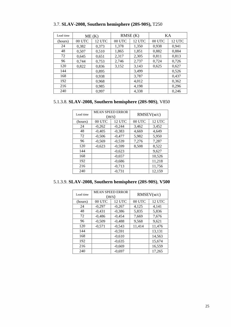
3.7. SLAV-2008, Southern hemisphere (20S-90S), T250



24 0,382 0,373 1,378 1,350 0,938 0,941

48 0,507 0,510 1,865 1,851 0,882 0,884

72 0,645 0,651 2,317 2,305 0,811 0,813

96 0,744 0,753 2,746 2,737 0,724 0,726

120 0,822 0,836 3,152 3,143 0,625 0,627

144 0,895 3,499 0,526

168 0,938 3,787 0,437

192 0,968 4,012 0,362

216 0,985 4,198 0,296

240 0,997 4,338 0,246

5.1.3.8. SLAV-2008, Southern hemisphere (20S-90S), V850


(m/s) RMSEV(м/c)


24 -0,262 -0,244 3,462 3,452

48 -0,405 -0,383 4,669 4,649

72 -0,506 -0,477 5,982 5,950

96 -0,569 -0,539 7,276 7,287

120 -0,623 -0,599 8,508 8,522

144 -0,623 9,627

168 -0,657 10,526

192 -0,686 11,218

216 -0,713 11,756

240 -0,731 12,159



(m/s) RMSEV(м/c)


24 -0,297 -0,267 4,125 4,141

48 -0,431 -0,386 5,835 5,836

72 -0,486 -0,454 7,669 7,676

96 -0,509 -0,488 9,568 9,621

120 -0,571 -0,543 11,414 11,476

144 -0,591 13,131

168 -0,610 14,563

192 -0,635 15,674

216 -0,669 16,559

240 -0,697 17,265

26



(m/s) RMSEV(m/s)


24 -0,472 -0,461 5,624 5,588

48 -0,758 -0,691 8,136 8,082

72 -0,934 -0,868 10,744 10,677

96 -1,042 -1,009 13,425 13,414

120 -1,184 -1,156 16,134 16,141

144 -1,253 18,670

168 -1,341 20,804

192 -1,415 22,572

216 -1,494 23,956

240 -1,567 25,074

27

5.2. Global Spectral Model of the Hydrometeorological Centre of Russia, version

T339L31

5.3.1. T339L31, 2015, Northern Hemisphere (20ºN – 90ºN)

5.3.1.1. T339L31, Northern hemisphere, Sea level pressure



24 -0,1 -0,1 1,9 2,0 0,97 0,97 0,34 0,35

48 0,0 0,0 2,9 2,9 0,94 0,93 0,43 0,44

72 0,1 0,0 3,9 4,0 0,89 0,88 0,52 0,53

96 0,0 5,2 0,80 0,62

120 0,0 6,4 0,70 0,69

144 0,0 7,4 0,60 0,76

168 0,0 8,2 0,50 0,80

192 -0,1 8,9 0,42 0,84

216 -0,1 9,6 0,35 0,86

240 0,1 10,1 0,28 0,88

5.3.1.2. T339L31, Northern hemisphere, H500



24 0,1 0,0 13,3 13,5 0,99 0,99 0,20 0,20

48 0,3 -0,6 23,0 23,6 0,97 0,97 0,28 0,28

72 0,9 -1,0 35,6 36,2 0,92 0,92 0,37 0,37

96 -1,7 50,7 0,85 0,46

120 -2,8 65,2 0,76 0,54

144 -3,7 78,5 0,65 0,60

168 -5,5 89,5 0,55 0,65

192 -6,5 99,0 0,45 0,69

216 -7,5 107,3 0,36 0,72

240 -8,4 114,4 0,28 0,74

5.3.1.3. T339L31, Northern hemisphere, H250



24 -0,2 -0,5 18,0 18,1 0,99 0,99 0,17 0,17

48 0,0 -0,9 31,7 32,1 0,97 0,97 0,25 0,25

72 -0,9 -1,3 48,7 49,2 0,93 0,93 0,33 0,33

96 -2,2 68,7 0,86 0,41

120 -3,9 88,9 0,77 0,48

144 -4,7 107,7 0,65 0,54

168 -6,7 123,8 0,57 0,58

192 -8,1 137,5 0,47 0,62

216 -8,9 149,0 0,38 0,65

240 -9,4 159,0 0,31 0,67

28

5.3.1.4 T339L31, Northern hemisphere, T500



24 0,0 0,1 1,1 1,1 0,95 0,95

48 -0,1 -0,1 1,5 1,5 0,91 0,91

72 -0,3 -0,3 2,0 2,0 0,84 0,84

96 -0,6 2,6 0,75

120 -0,8 3,1 0,65

144 -1,1 3,6 0,55

168 -1,3 4,1 0,46

192 -1,6 4,4 0,37

216 -1,8 4,8 0,30

240 -2,0 5,0 0,25

5.3.1.5. T339L31, Northern hemisphere, T250



24 0,7 0,7 1,4 1,4 0,92 0,92

48 0,8 0,7 1,9 1,9 0,84 0,84

72 0,8 0,8 2,4 2,4 0,76 0,76

96 0,7 2,8 0,66

120 0,5 3,1 0,57

144 0,3 3,3 0,49

168 0,1 3,5 0,42

192 -0,2 3,7 0,36

216 -0,4 3,9 0,32

240 -0,6 4,0 0,28

5.3.1.6. T339L31, Northern hemisphere, V500

Lead time MEAN SPEED

ERROR (m/s) RMSEV(м/c)


24 -0,3 -0,3 4,4 4,3

48 -0,3 -0,2 6,1 6,0

72 -0,2 -0,2 7,9 7,9

96 -0,2 9,7

120 -0,2 11,4

144 -0,2 12,8

168 -0,3 14,1

192 -0,3 15,0

216 -0,3 15,7

240 -0,3 16,2

29

5.3.1.7. T339L31, Northern hemisphere, V 250




24 -1.0 -0,9 6,2 6,1

48 -1,0 -1,0 8,7 8,6

72 -0,8 -0,9 11,4 11,3

96 -1,1 14,0

120 -1,1 16,5

144 -1,3 18,6

168 -1,4 20,6

192 -1,5 21,9

216 -1,6 23,0

240 -1,6 23,9

5.3.2 - T339L31., 2015 Tropics (20 N – 20 S)

5.3.2.1 - T339L31, Tropics, H850



24 0,5 0,4 7,2 7,6 0,86 0,86 0,49 0,52

48 0,6 0,4 8,9 9,0 0,84 0,82 0,52 0,55

72 0,6 -1,5 10,2 12,0 0,80 0,75 0,55 0,59

96 -1,6 13,6 0,71 0,61

120 -1,7 14,8 0,66 0,62

144 0,2 14,0 0,64 0,63

168 -1,9 16,6 0,58 0,66

192 -0,1 15,6 0,56 0,67

216 -2,2 18,0 0,51 0,69

240 -2,2 18,1 0,49 0,73

5.3.2.2 - T339L31, Tropics, H250



24 1,6 1,5 11,4 11,3 0,91 0,90 0,54 0,53

48 1,4 0,4 13,5 13,9 0,87 0,85 0,56 0,56

72 0,8 -0,9 15,8 16,7 0,82 0,81 0,59 0,59

96 -2,0 20,4 0,74 0,61

120 -4,0 24,2 0,68 0,64

144 -6,2 28,1 0,61 0,66

168 -8,5 31,8 0,53 0,68

192 -10,4 35,2 0,46 0,71

216 -12,2 38,1 0,40 0,72

240 -14,0 40,8 0,35 0,74

30

5.3.2.3 - T339L31, Tropics, T850



24 1,3 1,3 1,8 1,8 0,64 0,59

48 1,2 1,1 1,9 1,8 0,58 0,52

72 1,0 0,9 1,8 1,8 0,54 0,48

96 0,6 1,8 0,44

120 0,4 1,8 0,42

144 0,2 1,8 0,39

168 0,0 1,8 0,37

192 -0,2 1,9 0,34

216 -0,4 2,0 0,31

240 -0,6 2,1 0,29

5.3.2.4 - T339L31, Tropics, T250



24 0,9 0,8 1,2 1,2 0,74 0,71

48 1,4 1,3 1,7 1,6 0,65 0,62

72 1,5 1,3 1,9 1,7 0,60 0,57

96 1,2 1,7 0,50

120 0,9 1,6 0,44

144 0,6 1,4 0,40

168 0,2 1,4 0,36

192 -0,2 1,4 0,32

216 -0,6 1,5 0,30

240 -1,0 1,8 0,28

5.3.2.5 - T339L31, Tropics, V850




24 0,5 0,4 3,8 3,7

48 0,2 0,2 4,4 4,2

72 0,0 0,0 4,9 4,8

96 -0,2 5,2

120 -0,4 5,6

144 -0,5 5,9

168 -0,5 6,2

192 -0,6 6,4

216 -0,6 6,5

240 -0,6 6,7

31

5.3.2.1 - T339L31, Tropics, V250




24 -0,2 -0,3 5,9 5,9

48 -0,3 -0,3 7,3 7,3

72 -0,2 -0,3 8,4 8,4

96 -0,4 9,4

120 -0,5 10,2

144 -0,7 10,9

168 -0,9 11,7

192 -1,1 12,3

216 -1,2 12,8

240 -1,3 13,2

5.3.3. - T339L31, 2015, Southern Hemisphere

5.3.3.1 - T339L31, Southern Hemisphere, sea level pressure



24 -0,1 -0,2 2,8 2,9 0,96 0,96 0,29 0,30

48 -0,2 -0,2 3,8 3,8 0,94 0,93 0,37 0,38

72 -0,2 -0,3 5,0 5,0 0,90 0,89 0,46 0,46

96 -0,3 6,4 0,83 0,54

120 -0,3 7,7 0,75 0,61

144 -0,3 8,9 0,66 0,66

168 -0,3 9,9 0,58 0,70

192 -0,3 10,7 0,51 0,74

216 -0,2 11,4 0,44 0,76

240 -0,2 11,9 0,40 0,77

5.3.3.2 - T339L31, Southern Hemisphere, H500



24 0,9 1,1 16,7 17,7 0,98 0,99 0,18 0,18

48 0,6 0,8 28,1 28,6 0,97 0,97 0,26 0,26

72 0,6 0,7 42,1 41,1 0,92 0,92 0,34 0,34

96 0,7 58,7 0,86 0,42

120 0,7 74,2 0,77 0,48

144 0,7 89,7 0,67 0,54

168 1 101,9 0,57 0,58

192 -0,2 112,9 0,47 0,62

216 -0,5 122,7 0,38 0,65

240 -0,8 129,7 0,32 0,66

32

5.3.3.3 - T339L31, Southern Hemisphere, H250



24 0,6 0,8 22,2 22,5 0,99 0,99 0,16 0,16

48 -0,1 0,2 37,7 38,4 0,97 0,97 0,23 0,23

72 -0,3 0,1 55,7 56,8 0,93 0,93 0,30 0,30

96 0,3 77,2 0,86 0,37

120 0,3 97,6 0,78 0,43

144 0,2 118,1 0,68 0,48

168 -1,2 135,0 0,59 0,53

192 -1,9 150,3 0,49 0,56

216 -2,7 163,8 0,40 0,59

240 -3,5 173,7 0,33 0,61

5.3.3.4 - T339L31, Southern Hemisphere, T500



24 0,0 0,0 1,1 1,1 0,96 0,96

48 0,0 0,0 1,6 1,6 0,91 0,91

72 0,0 -0,1 2,1 2,1 0,85 0,85

96 -0,2 2,6 0,76

120 -0,4 3,1 0,66

144 -0,6 3,6 0,55

168 -0,9 3,9 0,45

192 -1,1 4,3 0,36

216 -1,3 4,6 0,29

240 -1,6 4,8 0,24

5.3.3.5 - T339L31, Southern Hemisphere, T250



24 0,5 0,5 1,4 1,4 0,92 0,92

48 0,5 0,5 1,9 1,9 0,84 0,85

72 0,5 0,4 2,2 2,2 0,77 0,77

96 0,3 2,6 0,69

120 0,0 2,9 0,61

144 -0,2 3,1 0,52

168 -0,5 3,4 0,45

192 -0,7 3,6 0,39

216 -1,0 3,8 0,34

240 -1,02 4,0 0,30

33

5.3.3.6 - T339L31, Southern Hemisphere, V500




24 -0,4 0,5 4,6 4,6

48 -0,3 0,5 6,6 6,6

72 -0,2 0,4 8,5 8,6

96 0,3 10,6

120 0,0 12,4

144 -0,2 14,1

168 -0,5 15,4

192 -0,7 16,4

216 -1,0 17,2

240 -1,2 17,8

5.3.3.1 - T339L31, Southern Hemisphere, V250




24 -1,0 -1,0 6,4 6,4

48 -0,9 -1,0 9,1 9,0

72 -0,9 -0,9 11,8 11,8

96 -1,0 14,7

120 -1,3 17,3

144 -1,4 19,8

168 -1,6 21,8

192 -1,8 23,4

216 -1,9 24,7

240 -2,0 25,6

Legend:

RMSE – root mean square error;

RMSEV – wind speed RMSE;

KA - anomaly correlation coefficient;

S1 – skill score

34

5.4 Verification of ensemble forecasts output

For assessment of the ensemble forecasts success, the probability estimates corresponding to

the requirements of the leading centre on verification of ensemble forecasts (Japan,

http://epsv.kishou.go.jp/EPSv/, Guideline on the Exchange and Use of EPS Verification Results,

http://epsv.kishou.go.jp/EPSv/guideline.pdf). Monthly averaged values are transmitted to the site of

the Centre of ensemble verification where they are presented in graphical format.

5.5 Research performed in this field

The forecast adaptation in localized areas close to the forecasting grid cells (fuzzy) and object-

oriented methods of mesoscale forecast verification adjustment to streams of operational radar

observation information formed with AKSOPRI complex developed in the Central Aerological

Observatory is under development. Main attention is paid to verification problems in

complicated mountainous relief considering meteorological support of the Sochi 2014

Olympic Games. Studies on variety of functions of precipitation patterns junction and coupling

(selected on the bases of the hourly accumulated precipitation threshold) are carried out using

statistical package R SpatialVx. Experiments are conducted for the period of forecast quality

assessment during Sochi 2014 Olympic Games (January 15 – March 15, 2014). It was

demonstrated that option of cutting off small objects (area is lesser than specified grid points)

is useful.

Operative implementation of unified verification system of short-range numerical forecasting

VERSUS-2 (jointly developed by the members of COSMO consortium), is supplemented with

blocks of probabilistic forecast quality calculation as well as calculation of confidence

intervals.

Development of the long-range forecasting verification systems:

Realization of the operational use of verification characteristics for long-range forecasting

recommended by WMO (2002) - the root mean quality (MSSS), relative operational

characteristic (ROC), reliability diagrams, and Derrity indicator in addition to standard

statistical characteristics (correlation coefficient, sign correlation, etc.). Inclusion of procedures

of cross-checking for stabilizing of quality assessment and broadening of forecasting fields

nomenclature for SLAV model version is planned for seasonal forecasts according to the

protocol of the project S2S.

Methods of parametric and non-parametric forecast significance assessment for long-range

forecasting schemes with different successfulness are developed and partly implemented using

the different statistical packages (IMSL, STATISTICA, R).

6. Plans for future (2016-2018)

6.1. Development of GDPFS

6.1.1. Main changes in operational GDPFS expected in 2016:

Operational implementation:

new version of SLAV model with horizontal grid step 20 km.

Improved version of the global spectral model T339L31.

Systems of ensemble short and medium-range forecasts based on three global

atmospheric models with approximately 70-km horizontal resolution using the

“breeding” method. 14 ensemble realizations.

http://epsv.kishou.go.jp/EPSv/

http://epsv.kishou.go.jp/EPSv/guideline.pdf

35

New version of COSMO-Ru technology with horizontal resolution 1 km for Moscow

and Sochi areas.

6.1.2. Main changes in operational GDPFS expected in 2017-2020

Implementation of cyclic assimilation for global models of the Hydrometeorologic Centre of

Russia.

Improvement and implementation of the new version of the semi-Lagrangian SLAV model

with spatial resolution 20-25 km and 50 vertical levels.

Implementation of new version of the global spectral model T339L63.

Implementation of the new version of ensemble medium-range forecasting system with

increased dimension of ensemble, expanded set of output products with improved post-

processing, which will include statistical correction.

Development of technological infrastructure (based on improved web-technologies) for

producing seasonal – inter-yearly forecasts for the territory of Russia. Implementation of

unified common technology of monthly and seasonal forecasting.

Development of the existing 3D-Var analysis scheme for the limited area forecasting model

(within the activities of COSMO consortium).

Assimilation of oceanographic data:

- Inclusion into assimilation system the data of satellite altimetery.

- Operative technology assimilation system implementation.

- Re-analysis of the hydrophysical oceanographic fields on the interval 2005-current.

- Increase the resolution of the global ocean circulation model.

6.2. Planned research in NWP, very short and long-range forecasting in 2016-2018

6.2.1. Planned research in NWP

- Data assimilation: Development of ensemble approach. Improvement of the local

ensemble Kalman filter with ensemble transformation (LETKF) for the SLAV model – gradual

introduction of satellite observations OSCAT/ASCAT and other. Development of mesoscale

assimilation system. Inclusion of the real statistics of the satellite observation errors.

- Global modeling: Improvement and renewing of the physical parameterizations in the

global models (spectral and finite-difference semi-Lagrangian models) for the new model

configurations. Development of the non-hydrostatic dynamic core for semi-Lagrangian

atmospheric model. Increasing of the SLAV model vertical resolution from 51 to 60 levels and

upper level of computational area from 5 to 1 hPa. Numerical experiments with the SLAV

model version 0,11х0,09 degrees, 60 levels. Implementation of the reduced lat-lon grid in the

full version of the SLAV model. Transfer to hybrid vertical coordinate. Improve stratospheric

block: ozone transport and photochemistry.

In the global spectral model – increase the number of vertical levels from 31 to 63.

- Ensemble forecasts: Two possible approaches to organization of future EPS are

investigated, in which initial data perturbations are prepared using a hybrid ensemble

variational data assimilation or a global LETKF. Tuning of statistical correction scheme.

- Development of the COSMO-RU system: improvement of the initial data preparation

blocks for underlying surface and lower layers of the atmosphere using the detailed synoptic

36

observations. Trial implementation of the mesoscale forecasting system based on COSMO-

Ru2 and version with the grid step 1 km for the Moscow region.

6.2.2. Planned research in long-range forecasting:

Improvement of SLAV model in long-range forecasting version (new

parameterizations, increased horizontal resolution - 0.9х0.72 degrees).

Experiments with coupled atmospheric model (SLAV) and ocean model

(INMOM) using the historic seasonal forecasts. Development of technology of

operational implementation of joint model;

Forecast of the meteorological extreme phenomena statistical characteristics;

Research of predictability dependence from the phases of large scale variability

modes;

Investigation on predictability while using different schemes of physical

parameterizations;

Investigation of predictability while using different schemes of hydrodynamic

models complexation.

Additional researches are planned within the framework of the North-Eurasian climate

centre (NEACC) projects.

1) Development of the average on-station forecasts using the super-ensemble NEACC

model with modified adaptation technique based on weekly discreetness of output model

product.

2) Inclusion of on-station forecast procedure for the territory of the former USSR into the

operational scheme of NEACC integrated for 90 days with weekly discreetness..

37

7. Participation in Consortiums

Russia (Roshydromet) is a member of the Consortium for Small-scale Modeling (COSMO).

7.1. Modeling system

7.1.1. In operation (see maps):

COSMO-Ru7 is a COSMO model version (grid step 7 km) adapted for the WMC Moscow

infrastructure covering the area from France to the west of Western Siberia in the zonal

direction and from the Barents and Kara Seas on the north to the Mediterranean Sea on the

south. The number of grid points is 700×620×40.

COSMO-RuSib is a COSMO-Ru version with a 14х14 km grid covering the area from

European Russia to the Far East and from the Arctic Ocean coast to the southern border of

Russia and Mongolia.

COSMO-Ru2cfo, COSMO-Ru2sfo and COSMO-Ru2vfo are COSMO model versions

(2.2х2.2 km) nested in the COSMO-Ru7 domain for the Central Federal District of Russia

(COSMO-Ru2cfo), the Northern Caucasia region (COSMO-Ru2sfo) and Volga region

(COSMO-Ru2vfo) respectively.

COSMO-Ru1SFO – version of the COSMO-Ru model, nested in COSMO-Ru2SFO –

horizontal grid step 1,1 km, Sochi region.

Domains of integration of the short-range forecasting system COSMO-Ru with resolution 13.2

km (COSMO-Ru13(ENA)), 7 km (COSMO-Ru7, blue rectangle), 2.2 km (COSMO-Ru2,

green rectangles), 1.1 km (COSMO-Ru1, red rectangle).

38

Integration domain of COSMO RuSib14

7.1.2. Research performed in this field

Developing a new configuration of COSMO-Ru with an integration domain covering

the whole territory of Russia with a 6.6-km step.

Activities within the COSMO working groups: WG1: development of data assimilation

technologies; WG3a: participating in the development of a new turbulence scheme

(shallow convection) for modeling with a resolution less than 2 km; WG3b:

development of a bog surface parameterization, development of a system for improved

calculation of snow water equivalent within the snow depth data assimilation system;

WG5: development of probabilistic score algorithms for ensemble forecast verification,

participation in INSPECT project aimed to compare different spatial methods of

verification; WG6: testing of new COSMO model versions; and WG7: development of

mesoscale ensemble modeling.

7.2. Systems run schedule and forecast ranges

COSMO-Ru13-ENA from 00 and 12 UTC: start +02-50, end +04-20, maximum lead time is

120 hours, products are issued with a 3h lead time step;

COSMO-Ru13-ENA: from 06 and 18 UTC, start +02-50, end +04-00, maximum lead time is

78 часов, products are issued with a 3h lead time step;

COSMO-Ru7: from 00 and 12 UTC: start +02-50, end +03-30, maximum lead time is 78

hours, products are issued with a 3h lead time step;

COSMO-Ru7: from 06 and 18 UTC: start +02-50, end +03-15, maximum lead time is 48 h,

products are issued with a 3h lead time step;

COSMO-Ru2cfo: from 00 and 12 UTC: start +03-40, end +04-15, maximum lead time is 24 h,


COSMO-Ru2cfo: from 06 and 18 UTC: start +03-15, end +03-50, maximum lead time is 24

h, products are issued with a 1h lead time step;

39

COSMO-Ru2sfo: from 00 and 12 UTC: start +04-20, end +05-25, maximum lead time is 48 h,


COSMO- Ru2sfo: from 06 and 18 UTC: start +03-50, end +05-10, maximum lead time is 48

h, products are issued with a 1h lead time step;

COSMO- Ru1sfo: from 00, 06, 12, and 18 UTC: start +01-05, end +01-25, maximum lead

time is 36 h, products are issued with a 1h lead time step;

COSMO- Ru2vfo: from 00, 06, 12, and 18 UTC: start +03-50, end +05-10, maximum lead

time is 48 h, products are issued with a 1h lead time step.

7.3. List of countries participating in the Consortium:

Germany, Switzerland, Italy, Greece, Poland, Rumania, Russia.

Each country supports its own technology based on the model codes provided by the

Consortium, the initial and boundary conditions from the Deutscher Wetterdienst or from the

European Centre for Medium-Range Weather Forecasts global models, and infrastructure

elements (verification, post-processing). The model software allows using the initial and

boundary conditions from a system of embedded grids.

7.4. Data assimilation, objective analysis and initialization

7.4.1. In operation

The results of the Deutscher Wetterdienst global data assimilation system are used; they are

provided for each initial time from the GME global modeling system (the grid step was 20 km

in 2014).

System of continuous observational data assimilation embedded into COSMO software is bsed

on “nudging” method.

7.4.2. Research performed in this field

Improvement of the nudging-based continuous data assimilation system supported by

the COSMO software for COSMO-Ru07 and COSMO-Ru02 by additional assimilation

of synoptic surface temperature measurements and temperature correction in the lower

atmospheric layers and upper soil layers. Analysis of efficiency of this system.

Adaptation of algorithms and technology of the 3D-Var global system of the WMC

Moscow for data assimilation within the COSMO-Ru systems.

7.5. Operationally available Numerical Weather Prediction products

7.5.1. In GRIB code:

A wide range of forecast products is provided in different vertical coordinates:

basic elements: temperature, wind speed, air humidity, geopotential heights at standard

isobaric surfaces, radiation fluxes;

one-level characteristics: of cloudiness at different levels, near-surface air

characteristics: air temperature at 2 meters, dew point at 2 meters, accumulated

precipitation, wind speed components and gusts at 10 meters, surface pressure and sea-

40

level pressure, heat and radiation balance components, snow depth and its water

equivalent;

GRIB messages are provided to users according to choice lists via FTP and to users’

addresses.

7.5.2. In graphical format

A) Maps

About 2000 maps for 00:00 UTC are automatically generated in GRADS and are distributed to

users via the Internet (FTP) and local networks:

-sea-level pressure + mid-level clouds+ 3h accumulated precipitation;

-500 hPa geopotential + near-surface air temperature+ sea-level pressure;

-near-surface background wind and its gusts;

stream function, 10m wind and gusts over the Baltic, Black, and Caspian seas;

-heights of convection boundaries and 500 hPa wind.

Selected graphical products are published in open access at:

http://meteoinfo.ru/cosmo-maps, http://metavia2.ru/main.php, http://sibnigmi.ru/cgi-

bin/inst/index.pl?5&2.

B) Meteograms:

Meteograms based on the GRADS visualization package are generated daily at the WMC

Moscow for 300 grid points in Russia and are distributed via FTP, Internet, and local networks

to users. Part of meteograms is in open access at http://www.meteoinfo.ru/-cosmo-ru.

7.6. Verification of prognostic products

Temperature and pressure, precipitation, cloudiness, wind speed and due point forecast quality

scores are regularly calculated based on the VERSUS-2 COSMO verification system for the

European part of Russia and the entire area covered by COSMO consortium countries.

Conditional verification is also carried out, i.e. calculation of the main weather elements under

prescribed meteorological conditions (limited or total cloud cover, etc.). Verification results

are presented on the site of COSMO consortium.

The forecast verification is made operationally using the WMC Moscow (Hydrometcentre of

Russia) verification system for 12-h accumulated precipitation, temperature, dew point,

background wind speed and wind gusts, and pressure (meteoinfo.ru).

7.7 Plans for the future (2016 – 2017):

7.7.1 Major changes in operational technology

To organize operational runs of COSMO-Ru model in new configuration for the

integration area including entire territory of Russia with a 6.6-km step (after installing

new hardware, previously the grid step was 13.2 km for technical reasons).

To implement into operation a system of data assimilation for snow water equivalent

using SYNOP data and snow depth and meteorological observations at the stations.

http://meteoinfo.ru/cosmo-maps

http://metavia2.ru/main.php

http://sibnigmi.ru/cgi-bin/inst/index.pl?5&2

http://sibnigmi.ru/cgi-bin/inst/index.pl?5&2

http://www.meteoinfo.ru/-cosmo-ru

41

7.7.2. Planned research activities:

Development of a COSMO-Ru modeling system with a 1-km step with modification of

the numeric method and physical parameterizations (primarily, the planetary boundary

layer and continuous data assimilation).

Development of parameterizations in the TERRA underlying surface model.

Development of turbulence parameterizations in the atmospheric planetary boundary

layer (PBL).

Further development of spatial methods of mesoscale model output verification.

Activities within the COSMO working groups according to the Consortium scientific

plan.

42

8. List of References

1. D.Alferov, E.Astakhova, D.Boukouvala, A.Bundel, U. Damrath, P. Eckert, F. Gofa,

A. Kirsanov, X. Lapillonne, J. Linkowska, C. Marsigli, A. Montani, A. Muraviev, E.

Oberto, M.S. Tesini, N. Vela, A. Wyszogrodzki, M. Zaichenko. Intercomparison of

Spatial Verification Methods for COSMO Terrain (INSPECT): Preliminary Results.

In: WMO/WGNE Research Activities in atmospheric and oceanic modeling, WCRP

Report No.15, 2015, pp.5-03-5-04.

2. Alferov D. Y., Е. D. Astakhova, G.S. Rivin, I.A. Rozinkina. Development of

ensemble forecasting system of high resolution for the Olympic Camesw Sochi 2014

region. Proceedings of the Hydrometeorological Centre of Russia, 2014, Iss. 352,

p.p. 5–20. [in Russian].

3. Astakhova E.D. Development of ensemble forecasting technologies. Thesis of

reports at VII All-Russian Meteorological Congress, July7-9, 2014 г, St.-Petersburg.

[in Russian].

4. Astakhova Elena, Andrea Montani, Dmitry Alferov, Dmitry Kiktev, Gdaly Rivin,

Inna Rozinkina, Chiara Marsigli, and Tiziana Paccagnella. Ensemble forecasts for

Sochi-2014 Olympics: development of COSMO-based ensemble systems and their

application. EMS Annual Meeting Abstracts.Vol. 11, EMS2014-235, 2014.

5. Astakhova E.D., A. Montani, D.Yu. Alferov. Ensemble forecasting system using the

COSMO model for the Sochi region: development of methods and securing of the

XXII winter Olympic Games with probabilistic forecasts. Proceedings of the

Hydrometeorological Centre of Russia, 2014, Iss. 352, p.p. 21–37. [in Russian]

6. Astakhova Е. D., G.S. Rivin, I.A. Rozinkina. Development of ensemble forecasting

system of high resolution for the Olympic Camesw Sochi 2014 region. Proceedings

of the Hydrometeorological Centre of Russia, 2014, Iss. 352, p.p. 5–20. [in Russian].

7. Kazakova E.V., Chumakov M.M., Rozinkina I.A. System of automated calculation

of snow water equivalent on the basis of numerical modeling and standard

meteorological observation data assimilation. // Proceedings of the Main

Geophysical Observatory (MGO), 2014, Iss.571, p.p. 114-133. [in Russian].

8. Kazakova E.V., Chumakov M.M., Rozinkina I.A. Calculation of the fresh snow

height using the results of atmospheric modeling (on COSMO-Ru example). //

Proceedings of the Hydrometeorological Centre of Russia, 2014, Iss.352, p.p. 74-84.

[in Russian].

9. Kazakova E.V., Chumakov M.M., Rozinkina I.A. Model for calculation of snow

cover characteristics based on observational data from standard meteorological

network. // Proceedings of the Hydrometeorological Centre of Russia, 2014, Iss.352,

p.p. 85-102. [in Russian]

10. Kazakova E.V., Chumakov M.M., Rozinkina I.A. Module for calculation of fresh

snow height depending on meteorological conditions using observations or numerical

forecast data – 6/12 accumulated precipitation. 2014. ROSPATENT. License

No.2014618542 dated 25.08.2014. [in Russian].

11. Kazakova E., Chumakov M., Rozinkina I. Initial fields of snow cover characteristics

preparation for COSMO-Ru // COSMO Newsletter No.14, 2014, р.p. 37-42.

12. Kazakova E.V., Chumakov M.M., Rozinkina I.A. Algorithm for calculation of fresh

snow height intend for post-processing of the atmospheric modeling systems. (on

COSMO example) // Proceedings of the Hydrometeorological Centre of Russia,

2013, Iss. 350, p.p. 164-179. [in Russian].

13. Kiktev Dmitry, Elena Astakhova, and Michael Tsyrulnikov. Field campaign and

information resources of the FROST-2014 project. EMS Annual Meeting Abstracts,

Vol. 11, EMS2014-272, 2014.

43

14. Kiktev D.B, E.Astakhova, A.Muravyev, M.Tsyrulnikov. Performance of the WWRP

project FROST-2014 forecasting systems: preliminary assesments. World Open

Science Conference-2014, Canada, Montreal. Book of abstracts, p.312. Available at http://wwosc2014.org/pdf/20140825-WWOSC-FinalBookofAbstracts.pdf

15. Kiktev D.B., Kruglova E.N., Kulikova I.A. Large-scale modes of atmospheric

variability.. Part 1. Statistical analysis and hydrodynamic modeling. Meteorology and

Hydrology, 2015, №3, p.p. 5-22. [in Russian].

16. Kiktev D.B., Khan V.M., Kryzhov V.N., Zaripov R.B., Kruglova E.N., Kulikova I.A.,

Tishenko V.A. Technology of long-range forecasts issuing in the Northern Eurasia

Climatic Centre (NEACC). Proceedings of the Hydrometeorological Centre of

Russia, Moscow,, М., 2015, Iss. 358, p.p.. 36 – 58. [in Russian].

17. Kulikova I.A., Kruglova E.N.,., Kiktev D.B. Large-scale modes of atmospheric

variability. Part 2. Their influence on spatial distribution of temperature and

precipitation on the territory of the Northern Eurasia. Meteorology and Hydrology,,

2015, №4, p.p. 5-16. [in Russian].

18. Lauritzen P. H., P. A. Ullrich, C. Jablonowski, P. A. Bosler, D. Calhoun, A. J.

Conley, T. Enomoto, L. Dong, S. Dubey, O. Guba, A. B. Hansen, E. Kaas, J. Kent,

J.-F. Lamarque, M. J. Prather, D. Reinert, V. V. Shashkin, W. C. Skamarock, B.

Sørensen, M. A. Taylor, and M. A. Tolstykh. A standard test case suite for two-

dimensional linear transport on the sphere: results from a collection of state-of-the-

art schemes. Geosci. Model Dev. 2014 v7. p. 105-145.

19. Mizyak V.G.,Shlyaeva A. V., Tolstykh M.A. Use of the satellite observational data

AMV in assimilation system based on LETKF. In Collection of articled

“International Youth Educational School and conference on numerical-information

technologies for environmental sciences, CITES–2015”, June 26-30, 2015, Tomsk,

Russia p.p. 137-141, ISBN 978-5-89702-389-395. [in Russian].

20. Montani A., D. Alferov, E. Astakhova, C. Marsigli, T. Paccagnella. Ensemble

forecasting for Sochi-2014 Olympics: the COSMO-based ensemble prediction

systems. COSMO Newsletters No. 14, 2014, pp. 88-94. Available at: http://cosmo-

model.org/content/model/documentation/newsLetters/newsLetter14/cnl14_10.pdf 21. Nikitin М.А., Rivin G.S., Rozinkina I.A., Chumakov M.M. Polar lows as an

unconsidered risk factor during marine operations in the Barents and Kara seas. V

International conference “Mastering of oil and gas resources of the Russian shelf:

Arctic and Far East”, October 29-30, 2014. – Moscow, Gazprom Vniigas, 2014.

22. Rogutov V.S., Tolstykh M.A. Assimilation and correction of radio sounding

humidity data in the data assimilation system on the basis of the local ensemble

Kalman filter. Russian Meteorology and Hydrology, 2015, Vol. 40, No. 4, p.p. 32-

45. [in Russian]

23. Rogutov V.S., Tolstykh M.A., Shlyaeva A. V. Use of the satellite wind observational

data at sea level ASCAT in the data assimilation system on the basis of the local

ensemble Kalman filter In Collection of articled “International Youth Educational

School and conference on numerical-information technologies for environmental

sciences, CITES–2015”, June 26-30, 2015, Tomsk, Russia p.p. 142-144. ISBN 978-

5-89702-389-395 [in Russian]

24. Strukov B.S., Resnyansky Yu.D., and Zelenko A.A. Ocean data assimilation with a

modified intermittent dynamic relaxation // Research Activities in Atmospheric and

Oceanic Modelling. Ed. by E. Astakhova. WCRP Report No. 12/2015. 2015. p. 8-

19–8-20.Тищенко В.А., Хан В.М., Толстых М.А. , Круглова Е.Н., Куликова

И.А., Гельфан А.М. Применение статистической коррекции месячных и

сезонных детерминистических прогнозов температуры воздуха и осадков по

модели ПЛАВ для отдельных районов России. Труды Гидрометцентра России,

М., 2015, вып. 358, с. 121 – 132. [in Russian]

http://wwosc2014.org/pdf/20140825-WWOSC-FinalBookofAbstracts.pdf

http://cosmo-model.org/content/model/documentation/newsLetters/newsLetter14/cnl14_10.pdf

http://cosmo-model.org/content/model/documentation/newsLetters/newsLetter14/cnl14_10.pdf

44

25. Tishenko V.A., Khan V.M., Tolstykh M.A., Kruglova E.N., Kulikova I.A., Gel’fan

A.M. Application of statistical correction to monthly and seasonal deterministic

forecasts of air temperature and precipitation in selected regions of Russia using

SLAV model. Proceedings of Hydrometeorological of Russia, М., 2015, Iss. 358,

p.p. 121 – 132.

26. Tolstykh M.A., N.A. Diansky, А.V. Guseb, D.B. Kiktev. Certain results of the

seasonal anomalies of atmospheric circulation simulation using the coupled model.

Proceeding of the Academy of Sciences of Russia, Physics of Atmosphere and

Ocean, 2014, Vol. 50, No.2, p.p. 131-142. [in Russian].

27. Tolstykh M.A, Fadeev R.Yu., Mizyak V.G., Shashkin V.V. Parallel program

complex of the atmospheric model for weather forecasting and climate modeling.

Collection of articles, International conference “Supercomputer Days in Russia”,

Moscow, September 28-29, 2015, Issued in MSU House, p.p. 356-367, available at

http://elibrary.ru/item.asp?id=24164037 [in Russian]

28. Tolstykh M.A., Volodin E.M., Fadeev R.Yu., Shashkin V.V. Multiscale version of

the global atmospheric model SLAV. In Collection of articled “International Youth

Educational School and conference on numerical-information technologies for

environmental sciences, CITES–2015”, June 26-30, 2015, Tomsk, Russia p.p. 59-62

ISBN 978-5-89702-389-395.

29. M. A. Tolstykh, J.-F. Geleyn, E. M. Volodin, N. N. Bogoslovskii, R. M. Vilfand, D.

B. Kiktev, T. V. Krasjuk, S. V. Kostrykin, V. G. Mizyak, R. Yu. Fadeev, V. V.

Shashkin, A. V. Shlyaeva, I. N. Ezau, A. Yu. Yurova. Development of the multiscale

version of the SLAV global atmosphere model. Russian Meteorology and

Hydrology, 2015, Vol. 40, No. 6, pp. 374–382. [in Russian]

30. Tolstykh M.A. Impact of snow albedo parameterization in the global atmospheric

model on medium- and long-range numerical forecasts. Proceedings of the

Hydrometeorological Centre of Russia, 2014, Iss. 352, p.p.139-149. [in Russian].

31. Vilfand R.M., Rivin G.S., Rozinkina I.A., Astakhova E.D., Blinov D.V., Bundel

A.Yu., Perov V.L., Surkova G.V., Alferov D.Yu., Kazakova Е.V., Kirsanov А.А.,

Revokatova А.P., Shatunova М.V., Chumakov М.М. Non-hydroststic system of the

Hydrometeorological Centre of Russia for mesoscale shoet-range weather forecast

using the COSMO-Ru model. – Collected articles: Turbulence, dynamics of

atmosphere and climate. Proceedings of International Conference in memory of

academician A.M. Obukhov (May 13-16, 2013) - Москва, GEOC, 2014, p.p. 265-

273. [in Russian].

32. Yurova A., M. Tolstykh, M. Nilsson, A.Sirin, Parameterization of mires in a

numerical weather prediction model // Water resources research. 2014. Vol. 50. p.p.

8982-8996.

33. . Zelenko A.A., Resnyansky Yu.D., Strukov B.S. Operational oceanography in the

Hydrometeorological Centre of Russia: status and prospective. //Proceedings of the

State Institute of Oceanography Named after N.N. Zubov. Studies of Oceans and

Seas. – 2015. –Iss. 21, p.p. 157–171. [in Russian]

34. Zelenko A.A., Strukov B.S., Resnyansky Yu.D., and Martynov S.L. Verification of

the wind wave forecasting system for the Baltic sea // Research Activities in

Atmospheric and Oceanic Modelling. Ed. by E. Astakhova. WCRP Report No.

12/2015. 2015 p.p. 8-23–8-24.

http://elibrary.ru/item.asp?id=24164037

Documents

FEDERAL SERVICE FOR HYDROMETEOROLOGY AND … · Semi-Lagrangian global model SLAV-2008 (jointly developed by the Hydrometcentre of Russia and the Russian Academy of Sciences), horizontal