Federal Land Managers' Air Quality Related Values ... · AIR QUALITY RELATED VALUES WORKGROUP (FLAG) ... The Federal Land Managers' Air Quality Related Values Work Group ... FLM actions

FEDERAL LAND MANAGERS’ AIR QUALITY RELATED VALUES

WORKGROUP (FLAG)

PHASE I REPORT (December 2000)

U.S. FOREST SERVICE – AIR QUALITY PROGRAM NATIONAL PARK SERVICE – AIR RESOURCES DIVISION

U.S. FISH AND WILDLIFE SERVICE – AIR QUALITY BRANCH

Table of Contents

A. EXECUTIVE SUMMARY .............................................................................................................iii 1. RECOMMENDATIONS FOR EVALUATING VISIBILITY IMPACTS .........................iv 2. RECOMMENDATIONS FOR EVALUATING OZONE IMPACTS.................................vii 3. RECOMMENDATIONS FOR EVALUATING DEPOSITION IMPACTS .......................ix

B. BACKGROUND ...............................................................................................................................1 1. HISTORY ....................................................................................................................................1

a. FLAG Approach .....................................................................................................................1 b. FLAG Organization................................................................................................................2

2. OVERVIEW OF RESOURCE ISSUES....................................................................................2 a. Visibility..................................................................................................................................3 b. Vegetation ...............................................................................................................................3 c. Soils and Surface Waters........................................................................................................4

3. LEGAL RESPONSIBILITIES ..................................................................................................4 4. COMMONALITIES AMONG FEDERAL LAND MANAGERS..........................................5

a. Identifying AQRVs ................................................................................................................6 b. Determining the Levels of Pollution that Trigger Concern for the Well-Being of AQRVs................................................................................................................................6 c. Visibility..................................................................................................................................6 d. Biological and Physical Effects..............................................................................................6 e. Determining the Level of Pollution Likely to Cause an “Adverse Impact” on AQRVs...............................................................................................................................7 f. FLM Databases ......................................................................................................................7

C. FEDERAL LAND MANAGERS' APPROACH TO AQRV PROTECTION................................8 1. AQRV PROTECTION AND IDENTIFICATION...................................................................8 2. NEW SOURCE REVIEW ...................................................................................................8

a. Roles and Responsibilities of FLMs .....................................................................................9 b. Elements of Permit Review .................................................................................................10 c. FLM Permit Review Process ..............................................................................................13 d. Criteria for Decision Making (Adverse Impact Considerations)........................................15 e. Air Pollution Permit Conditions that Benefit Class I Areas ................................................16 f. Reducing Pollution in Nonattainment Areas (Nonattainment Permit Process) ................17

3. OTHER AIR QUALITY REVIEW CONSIDERATIONS ...................................................17 a. Remedying Existing Adverse Impacts.................................................................................18 b. Requesting SIP Revisions to Address AQRV Adverse Impacts .......................................18 c. Periodic Increment Consumption Review ..........................................................................19

4. MANAGING EMISSIONS GENERATED IN AND NEAR FLM AREAS........................20 a. Prescribed Fire ......................................................................................................................20 b. Strategies to Minimize Emissions from Sources In and Near FLM Areas........................21 c. Conformity Requirements in Nonattainment Areas............................................................23

D. SUBGROUP REPORTS: TECHNICAL ANALYSES AND RECOMMENDATIONS...........24 1. SUBGROUP OBJECTIVES AND TASKS ............................................................................24 2. VISIBILITY...............................................................................................................................24 a. Introduction ...........................................................................................................................24 b. Analysis Techniques.............................................................................................................29 c. Air Quality Models and Visibility Assessment Procedures................................................29 d. Summary ...............................................................................................................................35

ii

e. Appendix 2.A Visibility Parameters ..................................................................................36 f. Appendix 2.B Estimate of Natural Conditions...................................................................40 g. Appendix 2.C Example Problem ........................................................................................69 3. OZONE .....................................................................................................................................75

a. Introduction ...........................................................................................................................75 b. Ozone Effects on Vegetation ...............................................................................................75 c. Recommended Metric to Determine Phytotoxic Ozone Concentrations ..........................77 d. Identification of Ozone Sensitive AQRVs or Sensitive Receptors ...................................79 e. Review Process for Sources that Could Affect Ozone Levels or Vegetation in

FLM Areas ...........................................................................................................................79 f. Further Guidance to FLMs ............................................................................................82

g. Ozone Air Pollution Websites.......................................................................................83 h. Appendix 3.A A Preliminary Listing for Selected USDA/FS, NPS, and FWS

Class I Areas of Plant Species that have been Shown to be Sensitive Receptors for Ozone...............................................................................................................................84 i. Appendix 3.B List of Representative Low and High W126 and N100 Values for SELECTED NPS and FWS Areas.........................................................................103

4. DEPOSITION..........................................................................................................................119 a. Introduction .........................................................................................................................119 b. Current Trends in Deposition.............................................................................................120 c. Identification and Assessment of AQRVs.........................................................................125 d. Determining Critical Loads ...............................................................................................129 e. Other AQRV Identification and Assessment Tools..........................................................132 f. Recommendations and Guidance for Evaluating Potential Effects from

Proposed Increases in Deposition to an FLM Area .........................................................134 g. Summary .............................................................................................................................142 h. Websites for Deposition and Related Information............................................................143

E. FUTURE FLAG WORK .......................................................................................................151 1. IMPLEMENTING FLAG RECOMMENDATIONS...........................................................151 2. PHASE I UPDATES...............................................................................................................151 3. PHASE II TASKS...................................................................................................................151

APPENDIXES A. GLOSSARY ..................................................................................................................................152 B. LEGAL FRAMEWORK FOR MANAGING AIR QUALITY AND AIR QUALITY EFFECTS ON FEDERAL LANDS .................................................................157 C. GENERAL POLICY FOR MANAGING AIR QUALITY RELATED VALUES IN CLASS I AREAS....................................................................................................166 D. BEST AVAILABLE CONTROL TECHNOLOGY (BACT) ANALYSIS ..........................168 E. MAPS OF FEDERAL CLASS I AREAS..............................................................................169 F. CLASS I AREA CONTACTS......................................................................................................173 G. FLAG PARTICIPANTS ..............................................................................................................195 H. BIBLIOGRAPHY..........................................................................................................................199

iii

A. EXECUTIVE SUMMARY The Federal Land Managers' Air Quality Related Values Work Group (FLAG) was formed to develop a more consistent approach for the Federal Land Managers (FLMs) to evaluate air pollution effects on their resources. Of particular importance is the New Source Review (NSR) program, especially in the review of Prevention of Significant Deterioration (PSD) of air quality permit applications. The goals of FLAG have been to provide consistent policies and processes both for identifying air quality related values (AQRVs) and for evaluating the effects of air pollution on AQRVs, primarily those in Federal Class I air quality areas, but in some instances, in Class II areas. Federal Class I areas are defined in the Clean Air Act as national parks over 6,000 acres and wilderness areas and memorial parks over 5,000 acres, established as of 1977. All other FLM areas are designated Class II. Maps of Federal Class I areas are provided in Appendix E. Lists of Class I Area contacts are provided in Appendix F. FLAG members include representatives from the three FLMs that administer the nation's Federal Class I areas: the U.S. Department of Agriculture Forest Service (USDA/FS), the National Park Service (NPS), and the U.S. Fish and Wildlife Service (FWS). (Subsequently in this report, these three agencies collectively will be referred to as “FLMs.” Class I and Class II air quality areas are called "FLM areas" in this report.) Appendix G contains a list of FLAG Participants. This report describes the work accomplished in Phase I of the FLAG effort. That work includes identifying policies and processes common to the FLMs (herein called “commonalities”) and developing new policies and processes using readily available information. This report provides State permitting authorities and potential permit applicants a consistent and predictable process for assessing the impacts of new and existing sources on AQRVs, including a process to identify those AQRVs and potential adverse impacts. The report also discusses non-new source review considerations and managing emissions in Federal areas. In Phase II, FLAG will address unresolved issues including those that will require research and the collection of new data. This FLAG Phase I Report consolidates the results of the FLAG Visibility, Ozone, and Deposition subgroups. The chapters prepared by these subgroups contain issue-specific technical and policy analyses, recommendations for evaluating AQRVs, and guidelines for completing and evaluating NSR permit applications. These recommendations and guidelines are intended for use by the FLMs, permitting authorities, NSR permit applicants, and other interested parties. The report includes background information on the roles and responsibilities of the FLMs under the NSR program. This document includes guidelines for completing and evaluating NSR applications that may affect FLM areas. It does not provide a universal formula that would, in all situations, allow one to determine whether or not a source of air pollution does, or would, cause or contribute to an adverse impact. That determination remains a project-specific management decision, the responsibility for which remains with the FLM, as delegated by Congress. The FLM's assessment of whether or not an adverse impact would occur is based on the sensitivity of the AQRVs at the particular FLM area under consideration. To provide information for the FLM’s assessment of adverse impacts on AQRVs, the permit applicant should identify the potential impacts of the source on all applicable AQRVs of that area. An FLM

iv

may ask that an applicant address any or all of the areas of concern. The primary areas of concern to the FLMs with respect to air pollution emissions are visibility impairment, ozone effects on vegetation, and effects of pollutant deposition on soils and surface waters. The FLAG Phase I Report also describes the FLAG effort–including the FLAG approach, organization, and plans for future FLAG work. Appendix A of the report contains a glossary of technical terms, abbreviations, and acronyms used in the report along with associated definitions. Appendix H provides a list of all references cited in the FLAG report. The key recommendations developed by the Visibility, Ozone, and Deposition subgroups are summarized below. However, for all three subject matter areas, FLAG recommends that the permit applicant consult with the appropriate regulatory agency and with the FLM for the affected area(s) for confirmation of preferred procedures. This consultation should take place in the early stages of the permit application process. 1. RECOMMENDATIONS FOR EVALUATING VISIBILITY IMPACTS FLAG has provided guidance in the form of recommendations, specific prescriptions, and interpretation of results for assessing visibility impacts of sources near Class I areas (although this guidance is generally applicable to Class II areas, as well). The guidance addresses assessments for sources proposed for locations near (generally within 50 km) and at large distances (greater than 50 km) from these areas. It also recommends impairment thresholds and identifies the conditions for which cumulative analyses of all increment-consuming sources would be necessary. The key components of the recommendations are highlighted below.

In general, FLAG recommends that an applicant:

• Consult with the appropriate regulatory agency and with the FLM for the affected Class I area(s) or other affected area for confirmation of preferred procedures and for the need for a cumulative analysis.

• Obtain FLM recommendation for the specified reference levels (estimate of natural conditions)

and, if applicable, FLM recommended plume/observer geometries and model receptor locations. • Apply the applicable EPA Guideline, steady-state models for regions within the Class I area that

are affected by plumes or layers that are viewed against a background (generally within 50 km of the source).

Calculate hourly estimates of ∆E and plume contrast, with respect to natural conditions, and compare these estimates with the thresholds given in Section D.2.c.

• For regions of the Class I area where visibility impairment from the source would cause a general

alteration of the appearance of the scene (generally 50 km or more away from the source or from the interaction of the emissions from multiple sources), apply a non-steady-state air quality model with chemical transformation capabilities (refer to IWAQM guidance documents), which yields ambient concentrations of visibility-impairing pollutants. At each Class I receptor:

v

Calculate the change in extinction due to the source being analyzed, compare these changes with the reference conditions, and compare these results with the thresholds given in Section D.2.c.

If necessary, calculate the cumulative change in extinction due to new source growth.

This prescription is portrayed schematically in Figure V-1.

vi

Figure V-1. Prescription for visibility assessment for distant/multi-source applications (source greater than or equal to 50 km from the Class I area)

Prescription for New Source Review Visibility Analysis

(Distant/Multi-source)

Single-source contribution to

change in extinction ≥

10.0% ?

FLM likely to object to the permit

FLM not likely to object to the permit

Has a cumulative analysis been conducted (or has the source

triggered a need for a cumulative impact analysis) or is its

contribution to extinction ≥ 5.0% ?

Conduct cumulative visibility analysis of PSD increment consuming sources

Cumulative change in extinction ≥10% and

single-source contribution ≥ 0.4%

?


Yes

No

No

Yes

Yes

No

vii

2. RECOMMENDATIONS FOR EVALUATING OZONE IMPACTS • FLAG agrees with the EPA contention that single source-receptor modeling for ozone is not

feasible at this time. FLM actions or specific requests on a permit application will be based on the existing air pollution situation at the area they manage. These conditions include (1) whether or not actual ozone damage has occurred in the area, and (2) whether or not ozone exposure levels occurring in the area are high enough to cause damage to vegetation (i.e., phytotoxic O3 exposures). Figure O-1 shows the various responses an FLM would have to a permit application. (Note: the term “Ozone exposure currently recognized as phytotoxic” is determined based on data from exposure response studies and ambient ozone levels at the site. The FLM may ask the applicant to calculate the ozone exposure values if these data are not already available. “Ozone damage to vegetation” is determined from field observations at the impacted site.)

• Oxidant stipple necrosis on plant foliage and ozone-induced senescence infer adverse

physiological or ecological effects, and are considered to be damage if they are determined to have a negative impact on aesthetic value.

• The W126 ozone metric is recommended to describe ozone exposure, based on a 24-hour,

seasonal (April through October) period of measurement. The number of hours in this period of time greater than or equal to 100 ppb (N100) will also be determined, in recognition of the importance of peak concentrations in plant response.

• NOx and VOC are of concern because they are precursors of ozone. Current information indicates

most FLM areas are NOx limited. Until we determine the VOC or NOx status of each area, we will focus on control of NOx emission sources.

viii

Figure O-1. FLM response to potential ozone effects from new emissions source.

No Unknown Unknown Yes Yes No Unknown Yes No Items referenced in Figure O-1: a. The FLM may recommend one or more of the following:

- That the proposed source use stricter than BACT controls (e.g., Lowest Achievable Emission Rate [LAER]). - That the proposed source obtain NOx emission offsets that will benefit the potentially affected FLM area (as demonstrated by dispersion modeling). - That the permitting authority (i.e., state or EPA) conduct regional modeling to identify sources that are contributing significantly to ozone-associated impacts in the FLM area, and that the permitting authority then undertake actions necessary to reduce emissions from those sources (e.g., SIP revision).

b. The applicant calculate the ozone exposure for vegetation (using W126 and N100 metrics) for the affected FLM area(s) where such information is not already available.

c. The permitting authority or applicant fund post-construction ambient ozone monitoring in or near the FLM area.

d. The applicant conduct or fund post-construction ozone effects surveys in the FLM area and/or exposure/response effects research.

a

FLM not likely to object to permit,; FLM may ask for d

FLM not likely to object to permit

Ozone damage to vegetation

FLM not likely to object to permit; FLM may ask for c and/or d

a; FLM may ask for c

FLM not likely to object to permit; FLM may ask for c

START

Ozone damage to vegetation a

Ozoneexposurecurrently

recognized asphytotoxic ; FLM

may ask for b

ix

3. RECOMMENDATIONS FOR EVALUATING DEPOSITION IMPACTS The permit applicant should consult with the appropriate regulatory agency and FLM for the affected area(s) to determine if a deposition impact analysis should be done. If an analysis is advised, the permit applicant should obtain available information on Class I AQRVs, critical loads, and concern thresholds from the FLM. In addition, the applicant should refer to the “Recommendations and Guidance for Evaluating Potential Effects from Proposed Increases in Deposition to an FLM Area” section of the Deposition Chapter (Section D.4.f). The following steps summarize that guidance. • Estimate the current deposition rate to the FLM area. A list of monitoring sites providing data to

characterize deposition in FLM areas is included in the Deposition Chapter (Table D-2). • Estimate the future deposition rate by adding the existing rate, the new emissions’ contribution to

deposition, and the contribution of sources permitted but not yet operating. Modeling of new and permitted but not yet operating emissions’ contribution to deposition should be conducted following IWAQM recommendations.

• Compare the future deposition rate with the recommended screening criteria (e.g., critical load,

concern threshold, or screening level value) for the affected FLM area. A list of documents summarizing these screening criteria, where available, can be found in Appendix H. Information for USDA/FS Class I areas is also available at:

http://www.fs.fed.us/r6/aq/natarm.

A website with NPS and FWS Class I area information is currently under development. • In consultation with the FLM, use the following flowchart (Figure D-1) to determine whether

mitigation is recommended.

x

No/Unknown

Yes

START

Current adverse

effects to AQRVsfrom deposition/

Critical load exceeded

?

Yes

Unknown

No

New emissions

cause or contribute to adverse effects/Critical

load exceeded?

FLM may recommendelements of "a" or "b"or (if necessary) "c"

a. The applicant should use one or more of the following: - Stricter (than BACT) controls (e.g., Lowest Achievable Emission Rate [LAER]). - Emission offsets located in an area that, considering geographic and meteorological factors, will benefit the impacted wilderness or park, as demostrated by modeling. - Regional modeling to identify sources contributing significantly to deposition adverse effects; SIP revision to reduce emissions contributing to adverse effects. (See text for discussion of mitigation options.) b. Deposition and deposition effects monitoring/research in the FLM area. c. Denial of permit.

FLM unlikely to object to permit

FLM unlikely toobject to permit;

may recommend "b"

Figure D-1. FLM resonse to potential deposition effects from new emissions sources.

Figure D-1. FLM response to potential deposition effects from new emissions sources.

B. BACKGROUND 1. HISTORY The Clean Air Act Amendments of 1977 give Federal Land Managers (FLMs) an “affirmative responsibility” to protect the natural and cultural resources of Class I areas from the adverse impacts of air pollution. (See Appendix B. “LEGAL FRAMEWORK FOR MANAGING AIR QUALITY AND AIR QUALITY EFFECTS ON FEDERAL LANDS.”) FLM responsibilities include the review of air quality permit applications from proposed new or modified major pollution sources near these Class I areas. If, in its permit review, an FLM demonstrates that emissions from a proposed source will cause or contribute to adverse impacts on the air quality related values (AQRVs) of a Class I area, the permitting authority, typically the State, can deny the permit. Individually, FLMs have developed different approaches to identifying AQRVs and defining adverse impacts on AQRVs in Class I areas. For example, in 1988, the U.S. Department of Agriculture Forest Service (USDA/FS) conducted a national screening process to identify the AQRVs for each of its Class I areas. Using this national process as a starting point, each USDA/FS region refined the screening parameters and identified sensitive AQRVs for many Class I areas. However, this resulted in differences in the approaches and levels used by USDA/FS regions. The U.S. Department of the Interior National Park Service (NPS) and the U.S. Fish and Wildlife Service (FWS) have adopted a case-by-case approach to permit review, considering the most recent information available for each area. NPS and FWS have not completed lists of sensitive AQRVs nor defined adverse impact levels for all of their Class I areas. a. FLAG Approach Air resource managers from the USDA/FS, NPS, and FWS recognized the need for a more consistent approach among their agencies with respect to their efforts to protect AQRVs. In April 1997, an interagency workgroup was formed whose objective was “to achieve greater consistency in the procedures each agency uses in identifying and evaluating AQRVs.” The workgroup named itself the Federal Land Managers' Air Quality Related Values Work Group, or FLAG. Although FLAG membership comprises air resource managers and subject matter experts from the three agencies, representatives from the U.S. Environmental Protection Agency (EPA), U.S. Geological Survey, and State air agencies have also participated in FLAG efforts. FLAG participants have collaborated to:

• define sensitive AQRVs, • identify the critical loads (or pollutant levels) that would protect an area and identify the

criteria that define adverse impacts, and • standardize the methods and procedures for conducting AQRV analyses.

To accomplish its objective, FLAG started with (and will continue to build on) the procedures, terms, definitions, and screening levels common to the three agencies. Many such “commonalities” were identified early in the FLAG planning sessions. (See section B.4. “COMMONALITIES AMONG FEDERAL LAND MANAGERS.”)

2

FLAG’s “Action Plan” stipulates a phased approach. Phase I addressed issues that could be resolved without research or the collection of new data. Phase II will address the more complex and unresolved issues from Phase I that may require additional data collection. (See section E. “FUTURE FLAG WORK.”) The FLAG effort focuses on the effects of the air pollutants that could affect the health of resources in Class I areas, primarily pollutants such as ozone, particulate matter, nitrogen dioxide, sulfur dioxide, nitrates, and sulfates. In Phase I, FLAG concentrated on four issues: (1) terrestrial effects of ozone; (2) aquatic and terrestrial effects of wet and dry pollutant deposition; (3) visibility impairment; and (4) process and policy issues. Four subgroups, one for each of these issues, were formed and charged with developing a set of recommendations for consistent policies and processes. In Phase I, FLAG findings and technical recommendations underwent scientific peer review, as well as review by agency decisionmakers such as Class I area Park Superintendents, Refuge Managers, and Forest Supervisors; Regional Foresters; and the Assistant Secretary for Fish and Wildlife and Parks. (Note: USDA/FS has designated the FLM as the Regional Foresters and, in some cases, Forest Supervisors. However, the Assistant Secretary for Fish and Wildlife and Parks holds FLM responsibilities for NPS and FWS.) FLAG products have also undergone public review and comment. [A “notice of availability” of the draft FLAG report was published in the Federal Register, and the FLMs conducted a public meeting to discuss the draft FLAG report and provided a 90-day public comment period.] b. FLAG Organization In addition to the four subgroups (policy, deposition, ozone, and visibility), the FLAG organization included Leadership and Coordinating Committees and a Project Manager. The Leadership Committee, which includes the air quality program chiefs from the three FLM agencies, was responsible for providing direction to the workgroup and the resources necessary for FLAG to accomplish its objective. The Coordinating Committee, which also includes representatives from each agency, was responsible for communications within the workgroup, including coordination among the agencies and subgroups. The FLAG Project Manager coordinated FLAG activities, served as a single point-of-contact for the subgroups, and performed other administrative functions. 2. OVERVIEW OF RESOURCE ISSUES Research conducted on Federal lands by FLMs and others has characterized natural resource effects associated with air pollution, and has helped identify those particular resources that are vulnerable to pollution. This effort does not address the impacts from air pollution on cultural resources. Documented effects include impairment of visibility, injury and reduced growth of vegetation, and acidification and fertilization of soils and surface waters. Air pollution effects on resources have been identified in a number of FLM areas; a few examples are provided below. It is important to note that similar, or even more serious, air pollution effects may be occurring on all Federal lands, but FLMs have not had the financial resources to perform the inventorying, monitoring, and/or research necessary to document such effects.

3

a. Visibility Visitors to national parks and wildernesses list the ability to view unobscured scenic vistas as a significant part of a satisfying experience. Unfortunately, visibility impairment has been documented in most Class I areas with visibility monitoring. Most visibility impairment is in the form of regional haze. The greatest visibility impairment due to regional haze occurs in the eastern United States and in southern California, while the least impairment occurs in the Colorado Plateau and Nevada Great Basin areas, and in Alaska. Sulfate is primarily responsible for visibility impairment in the eastern United States (e.g., Shenandoah National Park in Virginia); in southern California the majority of visibility impairment is attributable to nitrates (e.g., San Gorgonio Wilderness); in the Northern Rocky Mountains and Pacific Northwest, impairment is primarily due to organics (e.g., Glacier National Park in Montana); and in the intermountain West, sulfate, organics and elemental carbon are the main cause of impairment (e.g., Grand Canyon National Park in Arizona) (Sisler et al., 1993). Visibility impairment on Federal lands can also result from plume intrusion and has been documented in Mount Zirkel Wilderness, Moosehorn National Wildlife Refuge, and Grand Canyon National Park. b. Vegetation While several components of air pollution (e.g., sulfur dioxide, nitrogen dioxide, and peroxyacyl nitrates) can affect vegetation, ozone is generally acknowledged as the air pollutant causing the greatest amount of injury and damage to vegetation. The most common visible effects are stipple (dark colored lesions on leaves resulting from pigmentation of injured cells), fleck (collapse of a few cells in isolated areas of the upper layers of the leaf, resulting in tiny light-colored lesions), mottle (degeneration of the chlorophyll in certain areas of the leaf giving the leaf a blotchy appearance), necrosis (death of tissue), and in extreme cases, mortality. Aside from visible injury, ozone exposure can result in less obvious physiological impairment such as decreased growth or altered carbon allocation. Ozone fumigation experiments have identified a number of plant species that are sensitive to ozone. For example, fumigations were conducted in Great Smoky Mountains National Park (Tennessee and North Carolina) from 1987 to 1992. On the basis of foliar injury, thirty species were rated as sensitive to ozone levels that occurred in the park. The species with foliar injury included black cherry (Prunus serotina) and American sycamore (Platanus occidentalis). Additional observations and physiological measurements indicated elevated ozone reduced leaf, root, and total dry weights, and increased the severity of leaf stipple and premature leaf abscission in these two species (Neufeld and Renfro, 1993a,b). Field observations have documented foliar injury of these species in other eastern United States areas such as Brigantine Wilderness (New Jersey) and Cape Romain Wilderness (South Carolina). Ponderosa pine (Pinus ponderosa) and Jeffrey pine (Pinus jeffreyi) are recognized as good candidates for ozone-injury surveys in the western United States, based on their documented sensitivity. For example, these species were examined for ozone injury in national parks and national forests in the California Sierra Nevada from 1991 to 1995. The sites surveyed included Lassen Volcanic, Yosemite, and Sequoia/Kings Canyon National Parks and the Tahoe, Eldorado, Stanislaus, Sierra, and Sequoia National Forests. Foliar injury attributable to ozone was found at all areas, and the extent of injury generally increased in a southward direction along the Sierra Nevada (Miller et al., 1995).

4

c. Soils and Surface Waters

Acidity in rain, snow, cloudwater, and dry deposition can affect soil fertility and nutrient cycling processes in watersheds and can result in acidification of lakes and streams with low buffering capacity. Deposition of sulfate to sensitive watersheds results in leaching of base cations, soil acidification, and surface-water acidification. In some soils, sulfate adsorption results in "delayed" acidification of surface waters. Deposition of excess nitrogen species (nitrate and ammonium) to both terrestrial and aquatic systems can result in acidifying streams, lakes, and soils. There is also evidence that nitrogen deposition can cause shifts in phytoplankton composition in lakes in which biological activity is limited by nitrogen availability, i.e., increased nitrogen deposition can cause phytoplankton species that use nitrogen more efficiently to eventually dominate the lake. Water chemistry surveys and on-going monitoring show that many high elevation lakes on Federal lands in the Sierra Nevada, Cascades, and Rocky Mountains are sensitive to acid deposition. In general, these lakes are on bedrock that provides them with very little buffering capacity. Some of these lakes, for example, Loch Vale in Rocky Mountain National Park (Colorado) experience episodic acidification during Spring snowmelt (Baron and Campbell, 1997). Through funding provided by the Southern Appalachian Mountains Initiative, Herlihy et al. (1996) compiled information on surface water sensitivity of streams in nine of the eleven Class I areas in the Southern Appalachians. The nine Class I areas were grouped according to geology, physiography, and stream chemistry, then the groupings were ranked in terms of effects. Class I areas in the West Virginia Plateau (Otter Creek and Dolly Sods Wildernesses) had the highest percentage of acidic stream length and lowest pH values. Class I areas in the Northern and Southern Blue Ridge (e.g., Shenandoah National Park in Virginia and Joyce Kilmer/Slickrock Wilderness in North Carolina) had a lower percentage of acidic stream length, however, streams with low buffering capacity were common. The Alabama Plateau Class I area (Sipsey Wilderness) had streams with the highest buffering capacity. (Note that the authors based their report on surveys conducted by others and did not account for potential differences in methods of data collection.) A number of Federal areas contain estuarine and coastal areas that may experience eutrophication as a result of excess nitrogen deposition. For example, symptoms of eutrophication, including nutrient enrichment and algal blooms, have been observed in Everglades National Park and Chassahowitzka Wilderness (Florida). 3. LEGAL RESPONSIBILITIES

The specific legal responsibilities that Congress has given FLMs to protect natural, cultural, and scenic resources on the public lands from air pollution are identified in Appendix B. Statutes described in Appendix B. include agency organic acts, the Wilderness Act, and the Clean Air Act (CAA). The fundamental Congressional direction for managing public lands arises out of respective organic acts. Each of these laws is essentially a charter from Congress to the Executive Branch providing a purpose for parks, wildernesses, and refuges, respectively, and establishing broad management objectives for these areas. The Wilderness Act sets aside a subset of these public lands where natural processes are allowed to dominate. The agency stewards develop specific management objectives

5

building on the organic acts using public involvement, regulations, best available science, and additional direction provided by Congress. Among this additional Congressional direction is the Clean Air Act (CAA). It further characterizes some of the public lands as Class I areas and directs the land managers to take an affirmative responsibility to protect these areas from air pollution. The CAA directs that the FLMs identify and protect air quality related values, including visibility. This direction is consistent with the underlying charters provided by the organic acts and the Wilderness Act. The similarities of management objectives, and of the policies and procedures necessary for protecting Class I areas, are at the core of the FLAG process. In implementing laws, it is essential to understand the “intent of Congress.” In the case of the CAA, the FLM gleans additional insight from a passage in Senate Report No. 95-127, 95th Congress, 1st Session, 1977 which states,

“The Federal Land Manager holds a powerful tool. He is required to protect Federal lands from deterioration of an established value, even when Class I [increments] are not exceeded. … While the general scope of the Federal Government's activities in preventing significant deterioration has been carefully limited, the FLM should assume an aggressive role in protecting the air quality values of land areas under their jurisdiction. In cases of doubt the land manager should err on the side of protecting the air quality-related values for future generations.”

Although the FLMs have an "affirmative responsibility" to protect AQRVs, they have no permitting authority under the CAA, and they have no authority under the CAA to establish air quality-related rules or standards. The FLM role consists of considering whether emissions from a new source may have an adverse impact on AQRVs and providing comments to permitting authorities (States or EPA). It is important to emphasize that the FLAG report is only a guidance document that explains factors and information the FLMs expect to use when carrying out their consultative role. It is separate from Federal regulatory programs. The FLAG report describes the steps and process that the FLMs intend to go through in order to perform their statutory duties. Consequently, the scope of the FLAG report is to provide a more consistent approach for the three FLM agencies to evaluate air pollution effects on their resources, and to provide guidance to permitting authorities and permit applicants regarding necessary AQRV analyses. Although FLAG strives to be consistent with regulatory programs and initiatives such as the Regional Haze Rule and New Source Review Reform, no direct ties exist between FLAG and these regulatory requirements. 4. COMMONALITIES AMONG FEDERAL LAND MANAGERS If a new source is proposed near two or more areas managed by different FLMs, the FLMs generally try to coordinate in their interactions with the permitting authority and with the applicant. For example, two or more FLMs involved in pre-application meetings typically try to minimize the workload for the applicant by reaching agreement on the types of analyses the application should contain. Beyond coordinating during permit review, FLMs currently base requests and decisions on similar principles regarding resource protection and FLM responsibilities. Listed below are the

6

common principles in five areas of air resource management. In addition, Appendix C provides the FLM’s “GENERAL POLICY FOR MANAGING AIR QUALITY RELATED VALUES IN CLASS I AREAS.” a. Identifying AQRVs FLMs agree on the following definition of an AQRV:

A resource, as identified by the FLM for one or more Federal areas, that may be adversely affected by a change in air quality. The resource may include visibility or a specific scenic, cultural, physical, biological, ecological, or recreational resource identified by the FLM for a particular area.

This definition is compatible with the general definition of AQRV that appears in the Federal Register (FR 15016, April 10, 1978). That definition includes visibility, flora, fauna, odor, water, soils, geologic features, and cultural resources. FLMs have the responsibility to identify specific AQRVs of areas they manage. To this end, FLMs further refine AQRVs beyond the above definition to be more site-specific (i.e., area specific) by using on-site information. FLMs have developed inventories of specific AQRVs for many Class I areas and recognize that, ideally, inventories should be developed for all Class I areas. FLMs can be contacted for copies of site-specific AQRV lists. Finally, FLMs agree on the need for continued inventory, research, and monitoring to improve their ability to determine which AQRVs are most sensitive to air pollution and the sensitivity of these AQRVs. b. Determining the Levels of Pollution that Trigger Concern for the Well-Being of AQRVs FLMs believe that it should be possible to agree among themselves on the levels of pollution that trigger concerns for AQRVs. FLMs recognize the need to assess cumulative impacts and the difficulties associated with this process. Difficulties arise when a large number of minor source impacts eventually lead to an unacceptable cumulative impact or when a new source applies for a PSD permit in an area that has a high background concentration of pollution from existing sources. This means that a proposed new source should be evaluated within the context of the total impacts that are occurring or that potentially could occur from permitted/existing sources on the AQRVs of the area. c. Visibility FLMs use EPA-approved models to evaluate visibility impacts. The models use thresholds of visibility degradation measured in light extinction to evaluate source impacts to haze (far-field/multi-source impacts), and EPA established criteria for coherent plume impacts (near-field impacts). Currently all FLMs use Interagency Monitoring of Protected Visual Environments (IMPROVE) monitoring data to determine current conditions for visibility in FLM areas. d. Biological and Physical Effects All FLMs rely on research, monitoring, models, and effects experts to identify and understand physical, biological, and chemical changes resulting from air pollution and relating them to changes in AQRVs. Further, they focus on sensitive AQRVs (defined as either species or processes) to assess this biological/physical/chemical change.

7

e. Determining the Level of Pollution Likely to Cause an "Adverse Impact" on AQRVs FLMs rely on the best scientific information available in the published literature and best available data to make informed decisions regarding levels of pollution likely to cause adverse impacts. FLMs re-evaluate, update, and assess this information as appropriate. They consider specific Agency and Class I area legislative mandates in their decisions and, in cases of doubt, "err on the side of protecting the AQRVs for future generations." (Senate Report No. 95-127, 95th Congress, 1st Session, 1977) For air quality dispersion modeling analyses, FLMs follow 40 CFR §52.21(l) (Appendix W of Part 51, EPA's Guideline on Air Quality Models, revised 1996) and the recommendations of the Interagency Workgroup on Air Quality Modeling (IWAQM). FLMs recommend protocols for modeling analyses to permit applicants on a case-by-case basis considering types and amount of emissions, location of source, and meteorology. When reviewing modeling and impact analysis results, all FLMs consider frequency, magnitude, duration, and location of impacts. f. FLM databases Air Synthesis (formerly Air Quality Information Management System – AQUIMS) Air Synthesis is an information management and decision-support computer system under development by NPS and FWS. Air Synthesis is designed to assist FLMs in determining potential effects of pollutants on AQRVs. It contains information on air quality and its effects in Class I parks and wildernesses as well as natural resource data and annotated bibliographies of current literature on ozone and deposition. The system will also contain an interactive expert system module that will allow FLMs to assess the current status of freshwaters and determine if these resources are affected by deposition of sulfur or nitrogen. Natural Resource Information System – Air Module (NRIS-AIR) The Air Module is part of the USDA/FS’ Natural Resource Information System that integrates various physical, biological, and socioeconomic data within an integrated system of database, map-based spatial information, and analytical tools. Version 1.0 of NRIS-AIR, released in November 1998, tracks AQRVs, sensitive receptors, and indicators for each of the USDA/FS Class I areas. The water submodule provides data storage, reports, and tools for evaluating locally entered water quality and wet deposition data. Future NRIS-AIR versions (currently under development) will provide the information structure for visibility, flora, fauna, soil, geologic resources, cultural resources, and air quality data, as well as providing a PSD permit tracking system.

8

C. FEDERAL LAND MANAGERS' APPROACH TO AQRV PROTECTION FLM responsibilities for resource protection on Federal lands are clear and there should be no misunderstanding regarding the tools the FLM uses to fulfill these responsibilities. Opportunities to influence decisions regarding pollution sources external to the park or wilderness are limited. However, FLMs strive to minimize emissions from internal sources and their effects. Approaches for minimizing air pollution from external and internal sources are discussed in detail below. 1. AQRV PROTECTION AND IDENTIFICATION Congress assigned the FLMs an affirmative responsibility to protect AQRVs in Federal Class I areas. The FLMs interpret this assignment as a responsibility to:

1. Identify AQRVs in each of the Class I areas. 2. Establish inventorying and monitoring protocols for AQRVs. 3. Prioritize AQRV inventorying and monitoring (because of constrained budgets). 4. Specify a process for evaluating air pollution effects on AQRVs, including the use of

sensitive indicators. 5. Specify adverse effects for each AQRV.

To the extent possible, AQRVs have been identified for each Class I area. Additional AQRVs may be identified in the future as more is learned through science about the sensitivity of resources to air pollution. Public involvement in this process is necessary and will be accomplished through participation in the land management planning process or reply to an announcement in the Federal Register. While the sensitivity of an AQRV to air pollution may be known, the long term monitoring of its health or status may not have been accomplished. The expense of monitoring all AQRVs simultaneously is prohibitive. Consequently, FLMs seek opportunities through the permitting process and through partnerships to gather more information about condition of AQRVs. Because AQRVs themselves are often difficult to measure, surrogates are used as indicators, or sensitive indicators, of the health or status of the AQRV. Designing a working process for Class I area management and AQRV protection is outlined ahead in this document. Finally, an adverse impact is determined for each AQRV. An adverse impact from air pollution results in a diminishment of the Class I area’s national significance, that is, the reason the Class I area was created. Adverse impacts can also be an impairment of the structure or functioning of the ecosystem as well as an impairment of the quality of the visitor experience. The FLMs make an adverse impact determination on a case-by-case basis, based on technical and other information. 2. NEW SOURCE REVIEW Section 165 of the CAA spells out the roles and responsibilities for FLMs in New Source Review, including the Prevention of Significant Deterioration (PSD) permitting program. Other laws, such as the respective agency organic acts and the Wilderness Act, provide the fundamental underpinning of land management direction to land managers. The following discussion merges this complex

9

labyrinth of legal responsibilities as it relates to air resource management. A pending regulation revision from EPA which contains many of the items in this section addressing NSR may add more specificity to the Class I area protection process from the perspective of the CAA. a. Roles and Responsibilities of FLMs The FLM. The federal official directly responsible for the national parks, national wildlife refuges, and national forests (e.g., park superintendents, refuge managers, and forest supervisors, respectively) derive their responsibility from the respective agency organic acts. Furthermore, these officials, and the FLM for the respective agencies, have an affirmative responsibility under Section 165 of the CAA to protect and enhance the AQRVs of Class I areas from the adverse effects of air pollution. The FLM for the USDA/FS is the Regional Forester or the Forest Supervisor depending on the specific location. The FLM for the NPS and FWS is the Department of the Interior’s Assistant Secretary for Fish and Wildlife and Parks. Visibility Protection Program for New and Modified Sources. The FLMs have visibility protection responsibility under 40 CFR §51.307 (New source review), which spells out the requirements for State Implementation Plan (SIP) visibility protection programs, as well as 40 CFR §52.27 (Protection of visibility from sources in attainment areas) and 40 CFR §52.28 (Protection of visibility from sources in non-attainment areas). These three provisions, taken together along with the SIP-approved rules, establish the visibility protection program for new and modified sources throughout the country. Notification. Section 165 (42 USC, 7475) of the CAA requires the EPA, or the State/local permitting authority, to notify the FLM if emissions from a proposed project may impact a Class I area. The permitting authority should forward PSD applications to the FLM for review and analysis as soon as possible after receipt, giving the FLM an opportunity to review the application concurrently with the permitting authority. Generally, the permitting authority should notify the FLM of all new or modified major facilities proposing to locate within 100 km (62 miles) of a Class I area. In addition, the permitting authority should notify the FLM of "very large sources" with the potential to affect Class I areas proposing to locate at distances greater than 100 km. (Reference March 19, 1979, memorandum from EPA Assistant Administrator for Air, Noise, and Radiation to Regional Administrators, Regions I - X). Given the multitude of possible size/distance combinations, the FLMs can not precisely define in advance what constitutes a "very large source" located more than 100 km away that may impact a particular Class I area. Therefore, the FLM and permitting authority should work together to determine which PSD applications the FLM is to be made aware of in excess of 100 km. The FLM and permitting authority should make this determination on a case-by-case basis, considering such factors as:

• Current conditions of sensitive AQRVs; • Magnitude of emissions; • Distance from the Class I area; • Potential for source growth in an area/region; • Existing/prevailing meteorological conditions; • Cumulative effects of several sources to AQRVs.

10

Additionally, such dialogue facilitates coordination between permitting authorities and the FLMs. The significance of the impact to AQRVs is more important than the distance of the source. Not all PSD permit applications that the FLM is notified of will be analyzed in-depth by the FLM. FLM notification of a PSD permit application for a project located greater than 100 km does not mean that that application will be reviewed by the FLM in detail. Notification of PSD permit applications in excess of 100 km by the permitting authority allows the FLM to gauge the level of potential cumulative effects. As indicated above, the FLM decides which PSD permit applications to review on a case-by-case basis depending on the potential impacts to AQRVs. Pre-Application Meetings. To expedite the PSD permit review process, the FLM encourages pre-application meetings with permitting authorities and permit applicants to discuss air quality concerns for a specific Class I area in question. Given preliminary information, such as the source's location and the types and quantity of projected air emissions, the FLM can discuss specific AQRVs for an area and advise the applicant of the analyses needed to assess potential impacts on these resources. Completeness Determination. To further minimize delays, the FLMs encourage the permitting authority to use comments provided by the FLM concerning the completeness of the application, and to not deem the application complete until the applicant performs all necessary air quality impact analyses, including all relevant AQRV impact information. The permitting authority should then notify the FLM when they deem the application to be complete. Visibility Protection Procedures. Additional procedural requirements apply when a proposed source has the potential to impair visibility in a Class I area (40 CFR §52.27(d)(1998)). Specifically, the permitting authority must, upon receiving a permit application for a source that may affect visibility in any Class I area, notify the FLM in writing. Such notification should include a copy of all information relevant to the permit application, including the proposed source's anticipated impacts on visibility in a Class I area. The permitting authority should notify the FLM within 30 days of receipt and at least 60 days prior to the close of the comment period. If the FLM notifies the permitting authority that the proposed source may adversely impact visibility in a Class I area, or may adversely impact visibility in a previously identified integral (scenic) vista, then the permitting authority is to work with the FLM to address their concerns. If the permitting authority agrees with the FLM's finding that visibility in a Class I area may be adversely affected, the permit may not be issued. Even though the permitting authority may agree with the FLM's adverse impact finding regarding integral vistas, the permitting authority may still issue a permit if the emissions from the source are consistent with reasonable progress toward the national goal of preventing or remedying visibility impairment. In making this decision, the permitting authority may take into account the costs of compliance, the time needed for compliance, the energy and non-air quality environmental impacts of compliance, and the useful life of the source. The FLM will make a preliminary determination regarding possible adverse visibility impacts within a prescribed time of receipt of all relevant information. b. Elements of Permit Review The FLM review of a PSD application for a proposed project that may impact a Class I area generally consists of three main analyses:

11

1. Air quality impact analysis to ensure that predicted pollutant levels in Class I areas do not exceed National Ambient Air Quality Standards (NAAQS) and PSD increments, and to provide sufficient information for the FLM to conduct an AQRV impact analysis. Ensuring that permit applicants meet these requirements is the direct responsibility of the permitting authority (see discussion below);

2. AQRV impact analysis to ensure that the Class I area resources (i.e., visibility, flora,

fauna, etc.) are not adversely affected by the proposed emissions. The AQRV impact analysis includes interpreting the significance of the results from the applicant’s air quality impact analysis and is the responsibility of the FLM (see discussion below); and

3. Best Available Control Technology (BACT) analysis to help ensure that the source

installs the best control technology to minimize emission increases from the proposed project (See Appendix D for a summary of this analysis). The final BACT determination is a direct responsibility of the permitting authority.

Air Quality Impact Analysis. The permit applicant must perform an air quality impact analysis for each pollutant subject to PSD review. This analysis should show the contribution of the proposed emissions to increment consumption and to the existing ambient pollution levels in a Class I park or wilderness area. The applicant should perform a cumulative increment analysis for each pollutant and averaging time for which the proposed source will have a significant impact. Because proposed sources are not yet operating, the air quality analysis must rely on mathematical dispersion models to estimate the air quality impact of the proposed emissions. The FLMs provide the applicants with guidance on where to place model receptors within the Class I area. The applicant is responsible to provide sufficient information for the FLM to make a decision about the acceptability of potential AQRV impacts as a consequence of the new source. The applicant should perform the air quality impact analysis using approved models and procedures as specified in 40 CFR §52.21(l) and 40 CFR §51.166(l) (Appendix W of Part 51, EPA's Guideline on Air Quality Models, revised 1996 and in revision again as of the date of this writing, December 2000). The applicant should explicitly state all assumptions for the analysis, and furnish sufficient information on modeling input so that the FLM can validate and duplicate the model results. FLMs encourage the permit applicant to submit a modeling protocol for review before performing the Class I modeling analyses. This protocol should include the proposed air quality analysis methodology and model input (i.e., emissions, stack data, meteorological data, etc.), and the proposed location of the receptors in the FLM area. AQRV Impact Analysis. According to the CAA’s legislative history and current EPA regulations and guidance, the air quality impact analysis that provides sufficient information to enable the FLM to conduct the AQRV impact analysis is one part of a permit application just as are the BACT analysis and the air quality impact analysis relative to the increments and NAAQS. The applicant bears the entire cost of preparing the permit application including the complete air quality impact analysis. The FLM then uses the results from the applicant's air quality impact analysis and other information to conduct the AQRV impact analysis and make an informed decision about whether or not AQRVs will be adversely affected. If the FLM concludes that AQRVs are or will be

12

adversely affected, the FLM must so demonstrate to the permitting authority. The following sections of this document give guidance to applicants on how to conduct an air quality impact analysis and how the FLM uses this information to make an AQRV impact decision. Cumulative Impact Analysis. The applicant’s air quality impact analysis should include both the permit applicant’s contribution to the AQRV impacts, as well as the cumulative source impacts on AQRVs. A cumulative air quality analysis in which the proposed source and any recently permitted (but not yet operating) sources in the area are modeled is an important part of any AQRV impact analysis. This cumulative modeled impact is then added to measured ambient levels (to the extent that such monitoring data are available) so that the FLM can assess the total effect of the anticipated ambient concentrations on AQRVs. If no representative monitoring data are available, the applicant should estimate the total pollutant concentrations by modeling emissions from all contributing sources in the area. Information Provided by the FLM to the Applicant. To assist the permit applicant in performing air quality impact analyses, the FLMs will provide all available information about AQRVs for a particular Class I area that may be adversely affected by emissions from the proposed source. FLMs will recommend available methods the applicant should use to analyze the potential effects to the receptor(s) located in the Class I area. In addition to identifying AQRVs, FLMs will, to the extent possible:

(1) identify inventories, surveys, monitoring data, scientific studies, or other published reports that are the basis for identification of AQRVs;

(2) identify specific receptors known to be most sensitive to air pollution and the pollutant or pollutants that individually or in combination can cause or contribute to an adverse effect on each receptor;

(3) Identify the critical pollutant concentrations above which adverse effects are known or suspected to occur;

(4) Recommend methods the applicant should use for predicting ambient pollutant concentrations and other related impacts (e.g., deposition, visibility) which may cause or contribute to an adverse effect on each receptor; and

(5) Suggest screening level values or criteria that would be used to assess whether a proposed emissions increase would have a de minimis impact on AQRVs.

It is important to highlight the distinction between the air quality impact analyses that the applicant performs and the AQRV impact analyses that FLMs perform. Whereas the permit applicant calculates changes in pollutant concentrations, deposition rates, or visibility extinction, the FLM assesses the extent to which these impacts affect sensitive visual, aquatic, or terrestrial resources. Given the FLM’s statutory responsibilities and expertise, the FLM must have responsibility to consider whether the amount of pollution dispersed into the air or deposited on the ground (or in water) would have an adverse impact on any AQRV, and if so, to demonstrate that claim to the permitting authority. In making an adverse impact finding, FLMs consider such factors as magnitude, frequency, duration, location, and timing of impacts, as well as current and projected conditions of AQRVs based on cumulative impacts.

13

c. FLM Permit Review Process The FLM's current permit review process for any application that may impact a FLM area is described below. 1. Pre-application. If possible, participate in any pre-application meeting to learn specifics of the

proposed project (size, emissions, location, etc.) and to provide information regarding recommended Class I analyses.

2. Completeness Determination. Upon receipt, the FLM will review the application and

provide comments to the permitting authority regarding the completeness of the application and the need for additional information regarding the BACT, Air Quality Impacts, and AQRV Impacts analyses. The FLM will coordinate with the permitting authority and the permit applicant to ensure that all the necessary information to enable the FLM to make an impact determination is included.

3. Public Comment Period. After review of all relevant information, the FLM will provide

pertinent comments to the permitting authority, before or during the official public comment period, and/or at scheduled public hearings.

4. No Class I Increment Violated and No Adverse Impacts. If no Class I increment is

violated and no adverse impacts to AQRVs are expected, the FLM will inform the permitting authority of this determination and no further FLM action is necessary. The FLM may still provide BACT comments.

5. No Class I Increment Violated but AQRV Impact Uncertainty. If no Class I increment is

violated but uncertainty exists regarding potential adverse impacts to AQRVs, the FLM may request that the permitting authority include a permit condition that requires the permittee to conduct relevant post-construction AQRV or air quality monitoring. The FLM may also request certain control technologies or methods to reduce impacts.

6. Class I Increment Violated, but No Adverse AQRV Impacts. If the Class I increment is

violated, but no adverse AQRV impacts are anticipated, the applicant requests the FLM to "certify" no adverse impact under Section 165(d)(2)C)(iii) of the Clean Air Act [42 USC 7475(d)(2)(C)(iii)(1998)]. If the FLM concurs, (s)he makes a preliminary determination that no adverse impacts will occur.

a. The FLM will inform the applicant, the State/local permitting authority, and EPA of

the preliminary no adverse impact determination. b. The FLM will notify the public of its preliminary no adverse impact determination

either through the permitting authority's notice procedures, or through separate notice in the Federal Register. Such notice should include a statement as to the availability of

supporting documentation for inspection and copying, and an announcement of at least a 30-day public comment period on issues directly relevant to the determination in question. c. The FLM will review and prepare response to public comments.

14

d. The FLM will make a final determination regarding no adverse impacts, with a clear

and concise statement of reasons supporting that determination. e. The FLM will inform the permit applicant, the permitting authority, and EPA of its

final determination and if the final determination is "no adverse impact," the FLM shall so "certify" in a letter to the affected parties.

f. Simultaneous with step e, the FLM will publish a final determination in the "Notice"

section of the Federal Register, including a clear and concise statement of reasons supporting that determination, statement as to availability of supporting documentation for inspection and copying, and statement as to immediate effective date (date signed) of final determination.

g. The FLM will contact the permitting authority and request a revision to the State

Implementation Plan (SIP) to eliminate the Class I increment violations. 7. Adverse Impact Determination. Regardless of increment status, the FLM may make a

preliminary determination that the proposed project will cause, or contribute to, an adverse impact on AQRVs. Before officially declaring an adverse impact, the FLM will inform the proposed new source and the permitting authority that an adverse impact determination is imminent and suggest that the permit be modified. If the permit is modified to satisfy the concerns of the FLM, then an adverse determination is avoided.

a. The FLM will inform the applicant, the permitting authority, and EPA of a preliminary

adverse impact determination. b. The FLM will notify the public of the preliminary adverse impact determination either

through the permitting authority's notice procedures, or through separate notice in the Federal Register. Such notice should include a statement as to the availability of supporting documentation for inspection and copying, and an announcement of at least a 30-day public comment period on issues directly relevant to the determination in question.

c. The FLM will review and prepare response to public comments. d. The FLM will make a final determination regarding adverse impacts, with a clear and

concise statement of reasons supporting that determination. e. The FLM will inform the permit applicant, the permitting authority, and EPA of its

final determination. f. Simultaneous with step e, the FLM will publish a final determination in the "Notice"

section of the Federal Register, including a clear and concise statement of reasons supporting that determination, statement as to availability of supporting documentation for inspection and copying, and statement as to immediate effective date (date signed) of final determination.

15

g. If the FLM makes a final determination that a source will have an adverse impact, the FLM will oppose the permit. However, the permit applicant may propose to mitigate any adverse impacts (via reducing emissions, obtaining emission offsets, etc.). If the applicant adequately mitigates the adverse impacts to the satisfaction of the FLM, the FLM will withdraw his objection to the permit. If the adverse impacts are not adequately mitigated and the permitting authority nevertheless issues the permit, the FLM may appeal the permit.

Note: If the permitting authority's SIP makes execution of the above listed steps impossible (e.g., inadequate time allotments for the FLM's determination or lack of timely FLM notice ) the procedures shall be adjusted as appropriate. In addition, the above procedures (6 and 7) could also be modified to accommodate those situations when the FLM chooses to certify that existing impacts are adverse, absent a proposed new source. Such an action would alert potential permit applicants that adverse impacts exist and any new source would need to mitigate its potential impacts. Although each FLM may implement the above procedures somewhat differently, the FLAG goal is to reduce the differences in implementing the above steps. Furthermore, FLMs intend to coordinate on air permit modeling requirements for new or modified sources that are geographically near more than one FLM area. For example, a proposed source in eastern Tennessee that lies equidistant from NPS-administered Great Smoky Mountains National Park and the FS-administered Joyce Kilmer/Slickrock Wilderness would receive coordinated guidance on modeling requirements from the FLMs. The FLMs may or may not have common AQRVs at different Class I areas, making coordination beneficial. The FLMs may also coordinate on potential permit conditions and mitigation strategies. d. Criteria for Decision Making (Adverse Impact Considerations) As previously mentioned, the legislative history of the CAA provides direction to the FLM on how to comply with the affirmative responsibility to protect AQRVs in Class I areas, and in cases of doubt, the land manager should err on the side of protecting air quality-related values for future generations. The FLMs define adverse impact on AQRVs as:

An unacceptable effect, as identified by an FLM, that results from current, or would result from predicted, deterioration of air quality in a Federal Class I or Class II area. A determination of unacceptable effect shall be made on a case-by-case basis for each area taking into account existing air quality conditions. It should be based on a demonstration that the current or predicted deterioration of air quality will cause or contribute to a diminishment of the area's national significance, impairment of the structure and functioning of the area's ecosystem, or impairment of the quality of the visitor experience in the area.

Also, the Federal visibility protection regulations (40 CFR §51.300, et seq., §52.27) define adverse impact on visibility as:

[V]isibility impairment which interferes with the management, protection, preservation or enjoyment of the visitor's visual experience of the Federal class I area. This determination must be made on a case-by-case basis taking into account the geographic extent, intensity, duration, frequency, and time of visibility impairment, and how these factors correlate with: (1) times of

16

visitor use of the Federal class I area, and (2) the frequency and timing of natural conditions that reduce visibility. (Id. §51.301(a))

FLMs typically address adverse impacts on a case-by-case basis in response to PSD permit applications. When an adverse impact is predicted, FLMs recommend that permits either be modified to protect AQRVs or be denied. FLMs can also address adverse conditions outside of the PSD process. To do so, they: certify visibility impairment; participate in regional assessments; informally collaborate with States and EPA; review lease permits, SIP revisions, National Environmental Policy Act (NEPA) analyses, Park/Refuge/Forest management plans, CERCLA (Comprehensive Environmental Response, Compensation, and Liability Act) reviews, and other documents. In some States, FLMs use screening procedures or thresholds that indicate when the condition of an AQRV is acceptable or unacceptable. The pollutant concentration or loading rate that will adversely impact an AQRV can vary among Class I areas, and depends on current conditions. After a threshold is reached, an increase in pollutant concentrations is likely to be unacceptable. A concern threshold can be an adverse impact threshold or other quantifiable level in resource condition or pollutant exposure identified by the FLM. e. Air Pollution Permit Conditions that Benefit Class I Areas The FLM does not determine what permit conditions will be required or administer permit conditions; that is the responsibility of the permitting authority. However, the FLMs may request permit conditions or agree to withdraw objections to permit issuance if requested conditions are included. The FLMs view the inclusion of certain PSD permit conditions by the permitting authority as a means to help protect or enhance the condition of AQRVs when:

1. Air pollution source(s) may cause impacts that exceed protection thresholds for AQRVs;

2. Terrestrial resources, aquatic resources, and/or visibility are currently adversely impacted by air pollution and proposed emissions will exacerbate these adverse conditions;

3. FLM policies require improvement or restoration of AQRVs in parks and wildernesses; and

4. There is uncertainty on the extent and magnitude of air pollution effects on AQRVs. Permit conditions may require emission offsets, AQRV and/or air quality monitoring, inventories, re-openers, LAER (or other improved control technologies), or other measures to protect, enhance, or restore resources and values of parks and wildernesses. Permit conditions may:

1. Result in net air quality benefits at a protected area or within a region; 2. Contribute to a reduction of air pollution within a region; 3. Promote ecosystem inventories and/or monitoring to evaluate physical and biological

resource damage caused by air pollution emissions; and 4. Promote ecosystem restoration or improve the condition of resources damaged by air

pollution emissions.

17

The basis of an air permit condition may be identified in the public notice for the draft permit. To be effective, permit conditions must be federally enforceable and guaranteed. Air permit provisions may be temporary or permanent depending on the nature of the permit requirements. Procedures to implement an air permit condition must be acceptable to the FLM (e.g., an agreement between parties [memorandum of understanding, interagency agreement] is an option to accomplish inventory, monitoring, or other requirements). f. Reducing Pollution in Nonattainment Areas (Nonattainment Permit Process) The PSD program does not apply with respect to a particular pollutant when the source locates in an area designated non-attainment for that pollutant. Instead, pollution sources are regulated by Non-attainment Area New Source Review (NNSR). NNSR includes air quality planning and regulation of stationary sources. Air quality planning addresses issues such as lowest achievable emission rate (LAER), offsets, reasonably available control technology (RACT), and mobile and stationary source control strategies. New major stationary sources and major modifications of sources in designated non-attainment areas must satisfy NNSR before construction begins. For visibility protection, SIPs must include either EPA-approve provisions to comply with 40 CFR §51.307 for the non-attainment pollutant, otherwise, the federally promulgated visibility provisions at 40 CFR §52.28 would apply to all sources located in non-attainment areas. Therefore, FLMs can provide suggestions to the permitting authority regarding these conditions during the permitting and planning processes. SIPs provide a mechanism to address AQRV impacts for when the source or the Class I area is located in a non-attainment area. Land managers should recommend that States adopt policies, rules, or regulations in their SIPs requiring a demonstration that offsets will result in a net air quality benefit within any Class I area likely to be impacted by emissions from the source to be permitted. FLMs may also request emissions reductions greater than 1:1, perhaps offset rates of 1.5 or 2.0 to 1, or higher, depending on the impacts to be offset. Such recommendations can be developed jointly in a meeting with the regulatory authority or in a letter from the FLM. Mitigation measures recommended by FLMs may include stringent control technologies to minimize the increase in emissions and the impact on AQRVs. Monitoring can determine whether predicted resource conditions are observed. Offsets ensure that net emissions reductions from all sources will occur within a geographic area and their resulting air quality impacts at the Class I area will be mitigated. 3. OTHER AIR QUALITY REVIEW CONSIDERATIONS At all Class I areas where visibility has been monitored, visibility conditions have been found to be impaired (by human-caused pollution). The impairment comes primarily from older sources, not new sources. From a regional perspective, new or modified sources (using new/cleaner technologies) contribute far less to impaired AQRV conditions than old sources. New programs, such as EPA’s NAAQS for fine particulate matter and 8-hour ozone levels have been legally challenged (as of December 2000) so their effectiveness in reducing overall regional pollutant levels from older sources is uncertain at this time. EPA has implemented a call for reducing NOx emissions from older sources in the eastern U.S. to meet existing ozone standards, however, this action is being appealed to the U.S. Supreme Court. In addition to national ambient standards, most States are just now beginning the planning process to implement EPA’s Regional Haze Regulations. If all of these requirements are

18

implemented, then progress toward remedying impaired AQRVs is likely. However, given the sensitivity of some AQRVs to low levels of pollution, programs focused on reaching national goals, such as the NAAQS or visibility, may not fully remedy impacts on AQRVs in all locations. It is for this reason that the FLM should pursue all other reasonable strategies to protect AQRVs. The following sections discuss FLM issues that go beyond NSR. a. Remedying Existing Adverse Impacts The existence of adverse impacts is unacceptable to FLMs and contrary to the mandates of their specific agencies. Consequently, FLMs may request or participate in regional assessments to protect AQRVs, as appropriate. Regional assessments often use a multi-faceted approach to remedy impairment. For example, categories addressed by the Grand Canyon Visibility Transport Commission (GCVTC) include air pollution prevention; clean air corridors; stationary sources; sources in and near Class I areas; mobile sources; road dust; fire; and future regional coordination. Clean Air Act requirements for remedying existing visibility impairment provide a mechanism for addressing impacts from specific sources or groups of sources. Negotiations at the Centralia Power Plant in the state of Washington provide an example of how to build partnerships and work collaboratively to obtain retrofit controls or more stringent control technologies for sources that affect a FLM area. Through a collaborative decisionmaking process, owners of the Centralia plant agreed to reduce sulfur dioxide emissions at the plant by 90%. In another case, the USDA/FS asked the state of Colorado to remedy existing impairment at Mt. Zirkel Wilderness. Following USDA/FS testimony about the Mt. Zirkel Wilderness, terms of a court-ordered consent decree that specified controls for the Hayden Power Plant were included in Colorado’s long-term visibility strategy. FLMs may also coordinate with others to ensure that emission reductions in nonattainment areas will improve air quality in FLM areas. Recommendations on urban planning were developed with FLM involvement to address nonattainment areas in California. Data documenting ozone effects on vegetation were provided to the planning authority. b. Requesting SIP Revisions to Address AQRV Adverse Impacts A SIP is the key vehicle a state uses to develop the pollution control programs that will be used to achieve and maintain the NAAQS as well as prevent significant deterioration of air quality. It is important for FLMs to be involved in SIP development, as participation provides an opportunity to influence planning of pollution control programs that can benefit air quality in FLM areas. Once a SIP is fully approved by EPA, it is legally enforceable under both State and Federal law. FLMs can use the SIP process to address existing impacts that are unacceptable by requesting a SIP revision. This approach is particularly useful for addressing impacts on AQRVs other than visibility, since the Clean Air Act does not provide specific requirements for other AQRVs. In an October 16, 1996, letter from the Deputy Assistant Administrator of the EPA to the Assistant Secretary of the Department of the Interior (DOI), the EPA acknowledged that the CAA provides authority to address adverse impacts on AQRVs in Class I areas from both new and existing sources. EPA committed to initiate rulemaking that will set forth the affirmative obligation for States to protect AQRVs as part of their CAA responsibility to prevent significant deterioration of air quality. EPA states this approach would require the protection of AQRVs as part of SIPs.

19

In an October 17, 1996, response, DOI offered to assist EPA in developing this adverse impact SIP rulemaking. In addition, DOI urged EPA "to require State Implementation Plans to prevent significant deterioration of air quality by adopting mitigation measures to address adverse impacts on AQRVs in Class I areas." These SIP revisions could be used to address multiple sources and regional pollution that adversely affect AQRVs in all Class I areas. DOI sent a follow-up letter to EPA in July 2000 reiterating the need for an AQRV “restoration and protection” rulemaking. EPA solicited public input regarding an AQRV rule, as well as a request from Northeastern states for more stringent secondary NAAQS. EPA will consider comments received and then decide on a course of action. South Coast and San Diego, California, SIP revisions included FLM recommendations to reduce the impact of minor sources on AQRVs. South Coast recommendations addressed visibility while the San Diego recommendations addressed all AQRVs. EPA's NOX SIP Call in the east is another example of obtaining emission reductions through the SIP revision process. The NOX SIP Call is directed at 20 eastern States and the District of Columbia to address NOX emissions from existing large sources. Once this action is implemented, significant reductions in ozone formation and nitrogen deposition are anticipated. c. Periodic Increment Consumption Review As mentioned above, EPA has indicated its intention to the FLMs to establish a SIP revision requirement to address existing adverse impacts on AQRVs. The FLMs strongly support EPA exercising its authority in this way. In the interim, however, there are existing SIP revision requirements that are not being fully utilized. EPA's current regulations require States to conduct a periodic review of the adequacy of their PSD plan and program. [40 CFR §51.166(a)(4)] This would include an assessment of increment consumption in Class I and Class II areas. Few States have ever conducted a comprehensive, cumulative increment consumption analysis for one or more Class I areas. In addition, many PSD sources have not exceeded the significant impact levels for increment consumption; thus, few PSD permit applicants have had to perform a cumulative increment consumption analysis for Class I areas. Such a periodic increment consumption review would be beneficial given that the burden of proof for AQRV adverse impact determinations shifts from the FLM to the applicant when the increment has been consumed. In its 1990 report Air Pollution: Protecting Parks and Wilderness From Nearby Pollution Sources the U.S. General Accounting Office (GAO) found that only 1 percent of the sources within 100 kilometers of five Class I areas it investigated were required to have permits under the PSD program, with 99 percent of the sources being minor or grandfathered sources. It also found that “non-PSD sources contribute from 53 to 90 percent of five of the six criteria pollutants emitted within a 100-kilometer radius of each of the 5 Class I areas.” As part of its investigation, GAO noted that “a significant portion of total emissions of volatile organic compounds generally comes from small sources...and suggested that as part of the overall control strategy, States may want to consider lowering thresholds for regulating new sources to 25 tons of volatile organic compounds a year.” According to the investigation, 55 percent of anthropogenic VOC emissions come from new sources or modifications totaling 5 tons per year or less. In a review of PSD permit applications near Mesa Verde National Park (a Class I area in Colorado), a cumulative modeling analysis of increment-consuming sources found that approximately 80 percent of the NO2 Class I increment at the park had been consumed, but much of it by minor sources.

20

The FLMs have encouraged EPA to provide clearer direction on how often these periodic reviews must occur as the lack of a prescribed time-frame for conducting such analyses has clearly led to noncompliance with this requirement over the past twenty years by States. The FLMs believe EPA should revise 40 CFR §51.166 to require that the periodic reviews be conducted no less frequently than every five years. 4. MANAGING EMISSIONS GENERATED IN AND NEAR FLM AREAS Specific strategies need to be developed and implemented for reducing and preventing pollution from the many diverse sources and activities in communities surrounding FLM areas, including “gateway” communities. Accountability mechanisms are needed to ensure that appropriate actions are taken, reported and incorporated into SIPs, visibility protection plans, and Federal land management plans. Various forums (e.g., the Western Regional Air Partnership, and the Southern Appalachian Mountains Initiative) are addressing some of the emissions sources of concern and developing appropriate regional strategies. In addition, EPA has formed other “regional planning organizations” for implementing its regional haze rule. FLMs should participate in these forums, consistent with Federal law (e.g., Federal Advisory Committee Act), to the maximum extent possible and should coordinate their activities within those forums to ensure that comprehensive strategies are developed and implemented to address all the key emissions sources near FLM areas. A systematic assessment of emission sources in and near FLM areas would be extremely helpful for formulating strategies aimed at mitigating or eliminating adverse impacts on area resources. Without this assessment it is not possible to accurately quantify the extent to which these emissions contribute to the overall problem. Nevertheless, FLMs can, and should, take steps to minimize emissions generated on FLM lands even without an accurate inventory of emissions sources. a. Prescribed Fire Prescribed fire is a land management tool used for multiple landscape objectives. Prescribed fire allows the FLM to mimic natural fire return intervals under controlled conditions where smoke management can minimize air quality impacts. The alternative is wildfires, which can be very difficult to control and may cause much more severe air quality impacts. A modeling assessment suggests that using prescribed fire to minimize wildfires can result in a net reduction in fine particle (PM2.5) emissions in the long term. In the Pacific Northwest wildfire emissions were found to be greater than prescribed fire emissions in the same airshed (Ottmar, 1996). Since the turn of the century, wildfire has been aggressively suppressed on most of the nation's public lands to protect public safety, property, and to prevent what was thought to be the destruction of our natural and cultural resources. Fire-exclusion practices have resulted in forests, shrub lands, and grasslands plagued with a variety of problems, including overcrowding, resulting from the encroachment of species normally suppressed by fire; vulnerability of trees to insects and disease; and inadequate reproduction of certain species. In addition, heavy accumulation of fuels (such as dead vegetation on the forest floor) can cause fires to be catastrophic, which threatens firefighter and public safety, impairs forest and ecosystem health, destroys property and natural and cultural resources, and degrades air quality. The intense or extended periods of smoke associated with wildfires can also cause serious health effects and significantly decrease visibility.

21

FLMs recognize prescribed fire as a valuable tool; they also recognize that emissions from prescribed fire can be a significant source of air pollution. Smoke particles are also in the size range (< 2.5 µm) that they play a significant role in visibility impairment. Particulate matter is the main pollutant of concern from smoke because it can cause serious health problems, especially for people with respiratory illness. The FLMs are committed to minimizing the impacts from smoke by following sound smoke management practices, and if practical, using alternative methods to achieve land management objectives. Each prescribed burn site will have unique characteristics, but in general, smoke impacts can be greatly minimized by burning during weather conditions that provide optimal humidity levels and dispersion conditions for the type of materials being burned, in addition to limiting the amount of materials and acreage burned at one time. Generally, fire inside wilderness is considered natural–there is a need whenever possible to allow these fires to burn out naturally when the fires do not threaten private property or air quality conditions do not threaten human health. Visibility impairments caused by naturally ignited fires in wilderness should similarly be classified as natural. Unlike stationary source emissions, which are continuous, fire emissions are spatially and temporally sporadic. EPA has worked in partnership with land management agencies in the U.S. Departments of Agriculture, Defense, and the Interior; State Foresters; State air regulators; Tribes; and others to obtain recommendations and develop a national policy that addresses how best to improve the quality of wildland ecosystems (including forests and grasslands) and reduce threats of catastrophic wildfires through the increased use of managed fire, while achieving national clean air goals (U.S. EPA, 1998). EPA’s wildland fire policy describes criteria for wildland managers (federal, state, tribal, and private), and state and tribal air pollution agencies, to use in planning for and implementing prescribed fires, and recommends a variety of smoke management techniques that land managers can use to help reduce smoke impacts from prescribed fires. The policy is available at EPA’s website: http://www.epa.gov/ttn/faca/fa08.html. b. Strategies to Minimize Emissions from Sources In and Near FLM Areas Aside from prescribed fire, other activities that generate air pollution in FLM areas include road building, operation of generators, oil and gas development, etc. Developing strategies for addressing natural resource impacts in or near an FLM area should not only take into consideration the type of activities generating the emissions and their amount, but also the existing condition of the resources of that area. More stringent measures should be required for sources in and near FLM areas that are already experiencing adverse effects from air pollution. Examples of potential air pollution prevention practices that FLM agencies may encourage or develop and use are categorized under the following three strategies: Pollution Prevention Strategies Review land management plans for affected FLM areas to assess whether they include strategies to

limit and reduce air pollution emissions and incorporate protective measures into planning and decision documents.

Place priority on pollution prevention.

22

Encourage zero and near-zero emitting technologies. Promote energy conservation and the use of renewable energy sources. Promote use of clean fuels.

Mobile Source Strategies Promote the adoption of Low Emission Vehicle standards or the conversion of Federal fleets to

alternative fuels. Improve control of evaporative emissions. Adopt and enforce more stringent emission standards for the tour bus industry and other high-

emitting vehicles (e.g., snowmobiles). Retire high-emitting vehicles from Federal fleets as quickly as possible and/or relocate high-

emitting vehicles to less sensitive areas until they can be retired. Establish emission budgets from the transportation sector for selected FLM areas. Develop mass transit systems in some NPS units (e.g., light rail in Grand Canyon NP and a bus

system in Zion NP). Minor Source Strategies Apply RACT, BACT, LAER, best and reasonably available control measures, etc., to existing

sources, as appropriate. Go beyond conformity requirements to include the protection of AQRVs in FLM areas by

ensuring all actions FLMs can practicably control in and near FLM areas will not cause, or contribute to, an adverse impact on any AQRV.

Improved involvement with interested parties in gateway communities (those adjacent to FLM areas) will likely be required to ensure growth in these communities occurs in a manner that mitigates the impact on natural resources. These communities may need to enhance their participation in the planning processes of FLMs. Similarly, FLMs must participate in planning activities for public lands located in the FLM area and communities adjacent to FLM areas to ensure air quality concerns are adequately addressed. Mechanisms must be identified and developed for community involvement in developing, implementing, and enforcing emission management strategies for sources near and in FLM areas. Implementing strategies to achieve emission reductions in and near FLM areas will require efforts in at least three specific areas: 1. FLMs should ensure that sufficient emphasis is placed in agency planning documents requiring the

minimization of air pollution emissions from new activities or practices. 2. FLM agencies should inventory air pollution emissions within FLM areas. After emissions have

been quantified, FLMs, States, and adjacent communities will be able to assess the impact of these emissions through the use of appropriate models. Knowledge of Class I area emissions will also improve FLM ability to consult with States during the development and review of their SIPs (especially visibility SIPs).

3. FLMs should cooperate with States and local communities in assessing the need for, and the

development of, appropriate emission reduction strategies in and near FLM areas that address non-

23

PSD sources. Without an acknowledgment from States and local communities that these sources may pose a threat to FLM areas and a systematic assessment of these potential impacts, current efforts to protect FLM area resources may be insufficient.

c. Conformity Requirements in Nonattainment Areas Conformity criteria and procedures ensure that actions on lands administered by Federal agencies do not cause a violation of the NAAQS, increase the frequency of any standards violations, or delay attainment. Conformity to SIPs is only required for activities within nonattainment areas for non-transportation related sources if emissions are above de minimis levels and regionally significant. Any activity that represents 10 percent, or more, of the emission inventory for that pollutant in the non-attainment or maintenance area is regionally significant. Examples of actions that may require a conformity determination include road paving projects, ski area development, or mining. Activities such as prescribed fire, that are included in a conforming land management plan, are exempt from conformity requirements. The FLM should define the process to be used in conformity determinations and perform the conformity analysis before a project is implemented. A conformity analysis typically includes emission calculations, public participation, mitigation measures/implementation schedules, and reporting methods. The Pacific Southwest Region of the USDA/FS has published a Conformity Handbook for FLMs to assist in conformity compliance. In an approved Plan of Operation, FLMs can require monitoring. For example, in the case of Carlota Mine, located on National Forest land in Arizona, the USDA/FS requested additional mitigation measures to protect AQRVs in the Superstition Wilderness. Transportation projects in FLM areas classified as nonattainment are subject to a more complicated transportation conformity process. Consultation with State and local air quality and transportation agencies will be required to comply with applicable regulations.

24

D. SUBGROUP REPORTS: TECHNICAL ANALYSES AND RECOMMENDATIONS

1. SUBGROUP OBJECTIVES AND TASKS

Subgroups were formed to address the four key issues relevant to AQRV identification and evaluation issues: policy (and procedures), visibility, ozone, and deposition. Each of these subgroups reviewed the commonalities among the FLMs then addressed the tasks assigned to them by FLAG. One of their first tasks was to differentiate between Phase I tasks, those which could be resolved in the short term without significant additional resources, and Phase II issues, those that would require a longer period or greater effort. Subgroups were asked to reach common ground among the FLMs on the issues. The intent was to develop, to the extent possible, consistent policies, processes, and terminology that could be used when identifying AQRVs and evaluating impacts on AQRVs. This involves recommending consistent approaches for identifying air pollution effects on AQRVs, for determining adverse impacts, and for attributing adverse impacts to specific pollution sources. In addition, the FLMs consider that AQRV protection from visibility, ozone, and deposition impacts are equally important. However, we also recognize that given the current state of the science, attributing adverse impacts to specific sources are easier to document for visibility than for deposition and ozone, and easier for deposition than ozone. The individual subgroup reports document the common policies, procedures, and definitions identified or developed during Phase I activities. The Visibility, Ozone, and Deposition subgroup reports are included below. The FLAG Policy Subgroup Report was used as the basis for much of the rest of this FLAG Phase I Report, including much of Section B. "Background" and Section C. "Federal Land Managers' Approach to AQRV Protection." 2. VISIBILITY a. Introduction This chapter describes methods for analyzing the impacts on visibility from new or modified air pollution sources. This includes sources that fall under the purview of the Prevention of Significant Deterioration (PSD) regulations and sources that are being analyzed for Environmental Impact Statements under the National Environmental Policy Act (NEPA). The basis for some of the decisions outlined in this chapter is section 169A of the Clean Air Act. The opening statement of this section states: “Congress hereby declares as a national goal the prevention of any future, and the remedying of any existing, impairment of visibility in mandatory class I Federal areas which impairment results from manmade air pollution.” Under the regulations promulgated for visibility protection (40 CFR §51.301 (x)) visibility impairment is defined as “…any humanly perceptible change in visibility (visual range, contrast, coloration) from that which would have existed under natural conditions.” The remainder of this chapter describes methods that allow for new source growth to be analyzed against the constraint of preventing visibility impairment as defined in 40 CFR §51.301 (x), that is, new source growth should not allow any humanly perceptible change in visibility as compared against natural conditions. There are three different visibility impact thresholds that are discussed: levels of concern, analysis

25

thresholds, and decision thresholds. These are all interrelated. The levels of concern are visibility impact levels that would alert the FLM to a need for closer scrutiny. The analysis thresholds parallel these levels of concern in that if visibility impacts approach the levels of concern, the FLM would need to see further analyses to make an informed judgement about those impacts. The decision thresholds correspond to the visibility impacts, below which the FLM is not likely to object to an increase in visibility impairing pollutants. It is important to note that the decision thresholds can not be absolute; the FLM is required to make a determination on a “…case-by-case basis taking into account the geographic extent, intensity, duration, frequency and time of visibility impairments…” (40 CFR §51.301 (a)). However, the decision thresholds should be useful as an initial benchmark for analysts to judge whether visibility impacts would likely cause the FLM to object to a proposed action. Natural Conditions Comparing the impacts of new source growth against natural conditions implies that natural conditions are defined. At the time of this writing (December 2000) the EPA is working on defining natural conditions in support of their visibility regulations, but that work has not yet been completed. An estimate of natural conditions has been made (NAPAP, 1990). These estimates are only differentiated by the broad categories of the eastern and western United States. FLAG has adopted the appropriate aerosol concentrations from the NAPAP as estimates of natural conditions for each Class I area (Appendix 2.B). These estimates are a surrogate to be used until more definitive values for natural conditions are established. Visibility Impairment Before proceeding with the discussion, it is useful to identify the ways that visibility impairment can manifest itself. First, the pollutant loading of a section of the atmosphere can become visible, by the contrast or color difference between a layer or plume and a viewed background, such as a landscape feature or the sky. The second way that visibility is impaired is a general alteration in the appearance of landscape features or the sky, changing the color or the contrast between landscape features or causing features of a view to disappear. The first phenomenon is commonly referred to as plume impairment, whereas the second phenomenon is sometimes referred to as uniform haze impairment. As plumes are transported within a stable atmospheric layer, they may become a layered haze. As plumes and other more diffuse emission sources are transported and become well mixed in the atmosphere, they may develop into a uniform haze. Visibility Parameters The analysis methods for new source growth, described in this chapter, only deal with the visibility effects of discrete plumes and the aggregation of discrete plumes. The difference in these phenomena, as treated in this chapter, is whether the visibility effect is primarily seen as a section of the atmosphere which exhibits a change in contrast or color as compared with a viewed background, or whether the effect is due to an alteration of the appearance of the background features themselves. For the first situation, the contrast (C) and color difference index (∆E) of the plume and the viewing background are calculated. For the second situation, the change in atmospheric light extinction (∆bext), relative to natural conditions, is calculated. An approximation for which situation applies is the distance from the point of emission. (Distance serves as an indicator of where steady state conditions may apply.) The visibility impairment from sources

26

within 50 kilometers of a view is usually calculated using contrast and color difference, where visibility impairment from sources greater than 50 kilometers from a view, or the aggregation of a number of plumes, regardless of distance, is usually calculated using the change in light extinction. The distance approximation is useful for distinguishing these two phenomena; the terms “near field” and “distant/multi-source” are sometimes used in the remainder of this document to make this distinction. More information on visibility parameters can be found in Appendix 2.A. Levels of Concern The crucial level of concern for visibility impairment is whether it is humanly perceptible as compared against natural conditions (40 CFR §51.301(x)). As noted above, different visibility parameters are applied for different phenomena. A summary of the thresholds of perceptibility for the case of a plume viewed against a background indicates that contrast values (C) of ±0.01 to ±0.05 (note that the sign denotes whether the plume is brighter (+) or darker (-) than the background) are perceptible (NAPAP, 1990). A change in the color difference index (∆E) of less than 1 to 4 has been identified as the range of perceptibility for this parameter. The Workbook for Plume Visual Impact Screening and Analysis (USEPA, 1992a) suggests that a level of 0.05 for the absolute value of contrast (|C| = 0.05) and ∆E = 2 be used as thresholds in screening analyses; these levels were set in the mid-range of the perceptibility thresholds, in part, because of the conservative nature of the screening calculations. These levels also constitute the FLM’s level of concern for screening analyses of plumes viewed against a background. Under circumstances of a more refined analysis, |C| = 0.02 and ∆E = 1 are the levels of concern (USEPA, 1992b). These levels are usually applied for near field analyses where single sources are locating within 50 kilometers of a view. For the case of visibility impairment which changes the appearance of a viewed background feature, thresholds of perceptibility, where a just noticeable change occurs in the scene, have been found to correspond to a change in extinction (∆bext) as low as 2% under ideal conditions, up to 20% (NAPAP, 1990; Pitchford and Malm, 1994). A ∆bext of 5% will evoke a just noticeable change in most landscapes (NAPAP, 1990). The FLMs are concerned about situations where a change in extinction from new source growth is greater than 5% as compared against natural conditions. Changes in extinction greater than 10% are generally considered unacceptable by the FLMs and will likely raise objections to further pollutant loading without mitigation. These levels are usually applied for distant/multi-source analyses where sources are located more than 50 kilometers from a view or for analyzing the visibility impairment from an aggregation of plumes from multiple sources, regardless of distance. Cumulative Analyses A cumulative effects analysis of new source growth (defined as all PSD increment-consuming sources) on visibility impairment should be performed. The change in extinction (∆bext) will usually be the visibility parameter examined. The FLMs recognize that cumulative analyses of the effects of new source growth on visibility impairment have only rarely been carried out. Until cumulative analyses are performed for an area, the FLMs are suggesting some analysis thresholds to either trigger a cumulative analysis or allow a source to be permitted if its impact is below certain prescribed levels.

27

If a cumulative analysis has already been performed for the area, or if other considerations (i.e., NEPA, PSD increments, or other AQRV analyses) require that a cumulative analysis be performed for the proposed source, then the visibility impacts of the source are expected to be considered as part of the cumulative visibility impairment, as compared against natural conditions. When these conditions are met, the inclusion of the proposed source is expected regardless of the predicted visibility impairment of the source, unless its impacts are considered below de minimis. Analysis Thresholds for New Cumulative Analyses The analysis thresholds outlined here are interim levels to be used until such time as cumulative analyses are conducted for an area. Change in extinction (∆bext) is usually the visibility parameter analyzed for a cumulative analysis. If the visibility impact of a proposed project is below 0.4%∗ change in extinction, the impacts would be considered below de minimis and would not require further analysis. For situations where a cumulative visibility analysis has not been done or is not required because of other considerations, the following analysis thresholds will apply. If the visibility impact of a proposed source is less than a 5% change in extinction a cumulative analysis would not be expected. For visibility impairment predicted to be above 5%, but less than 10%, change in extinction from a proposed source, a cumulative analysis is expected. If the visibility impairment is predicted to be greater than 10% from a proposed source, the FLM is likely to object to the project regardless of other source growth, unless there is mitigation. Decision Thresholds Each determination of whether the impacts from a new source or major modification will be considered adverse must, by regulation, be made on a case-by-case basis (40 CFR §51.301(a)). Therefore, the decision thresholds specified here are strictly a guideline. More refined visibility analyses may indicate that the visibility parameters used (i.e., C, ∆E, ∆bext) do not adequately characterize the visibility for a particular situation; the FLMs will consider such information in making their decision. The decision thresholds parallel the FLM levels of concern. For near field situations where a section of the atmosphere is polluted and is viewed against a scenic background, screening analysis values of contrast with an absolute value less than 0.05 (|C| < 0.05) would not likely result in an objection by the FLM. Similarly, a value of ∆E < 2 from a screening analysis would not likely result in an objection. If a refined near field analysis is performed, values of |C| < 0.02 or ∆E < 1 would not likely result in an objection by the FLM. For distant or multi-source situations, if a cumulative visibility analysis has not previously been conducted and is not required for other analyses, a single-source change in extinction less than 5% would not generally trigger a need for a cumulative analysis. Under those circumstances, the FLM would not likely object to the proposed action. If the forecast single-source contribution to extinction is between 5% and 10%, or if a cumulative analyses is required or already exists, a special decision threshold applies. If the visibility impairment from the proposed action, in combination with cumulative new source growth, is less than a change in extinction of 10% for all time periods, the FLMs will not likely object to the proposed action. If the visibility impairment

∗ The de minimis level of 0.4% is defined as 4% of the unacceptable change in extinction (i.e., 10%), paralleling the discussion of significant impact levels in the proposed new source review modifications. (FR 61 38291-38293)

28

from the proposed action, in combination with cumulative new source growth, is greater than or equal to a change in extinction of 10% for any time periods, the FLMs will likely object to the proposed action, unless the contribution from the proposed action is less than a de minimis value of 0.4% for these time periods. Relationship to Regional Haze Rule The FLAG recommendations are complimentary to the regional haze rule. However, the visibility recommendations of FLAG are intended for new source review and NEPA type applications, whereas the regional haze rule addresses the effects of existing sources of visibility impairment in conjunction with new source review. The FLAG recommendation is designed to prevent new sources from causing visibility impairment, and the criteria for developing these recommendations do not necessarily apply to existing sources. At the time of this writing, new source review is an ongoing effort, but it will be several years before State Implementation Plans (SIPs) under the regional haze rule are submitted. If the new visibility SIPs adequately account for new source growth, the FLMs may reconsider the FLAG recommendations. The visibility parameters for cumulative impact analysis, outlined here, are related to those in the regional haze rule. However, an assumption inherent in regional haze is that the pollution is fairly evenly distributed over a broad geographic extent. By contrast, the analysis techniques, described herein, at most deal with the aggregation of a subset of the plumes that might affect regional haze, but do not meet the criteria of being a regional haze. The levels of concern and de minimis levels described in this document were arrived at, in part, with the knowledge they apply to a limited number of sources under new source review and that the analyses are always compared to natural conditions. The de minimis levels described here should not be used for determining whether emissions from an existing source are reasonably anticipated to cause or contribute to visibility impairment. Those criteria have been laid out in the regulations (40 CFR §51 Subpart P Protection of Visibility) and through interpretations of those regulations by EPA and courts. While there are some distinct differences between this document and the regional haze rule, there are also some similarities. One of these is the need for conducting a cumulative assessment of visibility impairment. This will include the need for evaluating the effects of sources beyond an individual state’s boundaries. Therefore, it is anticipated that when modeling centers are established for SIP development work, the tools they use may be applicable to analyzing both existing impairment as well as the potential impacts of new source growth.

29

b. Analysis Techniques There are two fundamentally different approaches one could adopt to determine visibility impairment. One is a technically rigorous, complex, and situation-specific method, while the other is a more generalized approach. The more rigorous approach requires determination of particle concentrations and size distributions, calculation of particle growth dynamics, and application of Mie Theory to determine the optical characteristics of the aerosol distribution. Sophisticated radiative transfer models are then applied, using aerosol optical characteristics, lighting and scene characteristics, and spatial distribution of the pollutants to calculate the path and wavelength of image-forming and non-image-forming light that reaches a specific observer from all points in the scene being viewed.

While such a detailed analysis may be useful for assessing specific cases, it is usually impractical for situations in which visibility could be experienced in a nearly infinite variety of circumstances. Practical limitations frequently dictate that it is more reasonable to use a generalized approach to determine the change in extinction by using bulk-averaged aerosol-specific extinction efficiencies rather than trying to reproduce the complex optical phenomena that may occur in the atmosphere.

Consequently, FLAG recommends the generalized approach for determining the effects on visibility from a proposed new source's emissions. The procedure is to estimate the atmospheric concentrations of visibility impairing pollutants, apply representative visibility parameters, calculate the change from specified reference levels, and compare this change with prescribed threshold values.

FLAG is using estimates of natural conditions as reference levels for Class I visibility analyses. Comparison with natural conditions will help ensure that those conditions will not be impaired in keeping with Section 169A of the CAA. Because of the different requirements of the two modeling approaches discussed below, natural conditions must be expressed using two different metrics:

• Standard visual range (visual range adjusted to a Rayleigh condition of 10 Mm-1), for near field modeling. Present EPA guideline visibility models traditionally accept visibility conditions expressed in these terms.

• Extinction, for distant/multi-source modeling. Visibility conditions should be expressed in terms of the averaged extinction efficiencies of the individual atmospheric constituents that comprise the total extinction. The relative humidity effects of the hygroscopic particles must be accounted for when the change in extinction is calculated.

Information needed to calculate the above indices is provided in Appendix 2.B for all 156 Class I areas for which visibility is an important attribute. If estimates are needed for Class II areas, the FLM can provide them.

c. Air Quality Models and Visibility Assessment Procedures The modeling discussion will be divided into two parts to address the very different requirements for 1) near field modeling where plumes or layers are compared against a viewing background and 2) distant/multi-source modeling for plumes and aggregations of plumes that affect the general appearance of a scene. Note that both of the above analyses might apply depending on the source’s

30

proximity to all portions of the Class I area or multiple Class I areas. Near Field Analysis Technique for Analyzing Plumes or Layers Viewed Against a Background The Model (Near Field – Steady State Conditions Applicable) EPA has recommended a methodology to assess impacts due to coherent plumes. A guideline, for when these steady state conditions apply, is the distance from the source to the view of concern. This technique is usually applied for sources locating less than 50 km from a Class I area. Applicants must model their potential plume impacts using the screening model, VISCREEN (USEPA, 1992a), or, if the next level of analysis is called for, PLUVUE II (USEPA 1992b and 1996c). Both of these models use steady-state, gaussian-based plume dispersion techniques to calculate one-hour concentrations within an elevated plume. These two models calculate the change in the color difference index (∆Ε) and contrast between the plume and the viewing background. Values of ∆Ε and plume contrast are based on the concentrations of fine primary particulates (including sulfates), nitrogen dioxide (NO2), and the geometry of the observer, target, plume, and the position of the sun. PLUVUE II also allows consideration of the effects of secondarily formed sulfates. Plume contrast results from an increase or decrease in light transmitted from the viewing background through the plume to the observer. The specifics of the emission scenarios and plume/observer geometries for modeling should be selected in consultation with the appropriate FLM. At the present time there is no recommended procedure for conducting analyses of multiple sources with these modeling tools, so multiple coherent plumes must be treated individually, or combined into a representative single source if reasonable. The Recommended Prescription (Near Field – Steady State Conditions) Until better modeling tools are available, FLAG recommends using the present EPA techniques for plume visual impact screening analyses (USEPA 1992a). However, unlike those procedures, which suggest the use of current average annual visibility conditions, FLAG recommends that the visual range corresponding to natural conditions be used to generate the hourly estimates of ∆E and plume contrast. FLAG recommends this change in order for the analysis technique to be consistent with the national visibility goal. For screening-level analyses, FLAG recommends the use of the annual average reconstructed natural conditions given in the last column in Table 2.B-1 in Appendix 2.B. The table entry gives the specified reference level (including the effects of relative humidity) expressed in Mm-1. The conversion to standard visual range can be made using Equation 1 in Appendix 2.A. For the refined analyses, the reconstructed natural condition is derived from the relative humidity used in the modeling, the corresponding relative humidity adjustment factor (Table 2.A-1), and estimated natural aerosol concentrations (Table 2.B-1). If a screening analysis of a new or modified source can demonstrate that its emissions will not cause a plume with any hourly estimates of ∆E greater than or equal to 2.0, or the absolute value of the contrast values (|C|) greater than or equal to 0.05, the FLM is not likely to object to the issuance of the PSD permit based on near field visibility impacts and no further near field visibility analyses will be requested. More refined analyses (i.e., PLUVUE II) would be undertaken if the above conditions are not met and would be compared against lower levels of concern; the FLM would not likely object if ∆E < 1.0 and |C| < 0.02.

31

If the estimated plume parameters exceed the aforementioned values, the FLM would rely on a case-by-case effects-based test (NPS 1993), taking into account magnitude, frequency, duration, and other factors, to decide whether to make an adverse impact determination. Distant/Multi-Source Techniques for Analyzing Whether a Plume or an Aggregation of Plumes Alters the General Appearance of a Scene This application is generally more complex than the near field, coherent plume modeling analyses and the guidance from EPA is less definitive, though it is evolving. The modeling system must include the capability to assess single and multiple sources in a temporally and spatially varying meteorological domain, accommodate modeling domains measuring hundreds of kilometers, include rough and complex terrain, provide pollutant concentration estimates for averaging times from one-hour to annual, and address inert and secondarily formed pollutants and dry and wet deposition. In the early 1990s the FLMs and the EPA recognized the need for a consistent, technically credible technique to estimate contributions to air quality of multiple new sources locating more than 50 km from Class I areas. Toward that end, the Interagency Workgroup on Air Quality Modeling (IWAQM) was established to develop a modeling protocol for this application. FLAG proposes to rely on the IWAQM recommendations and modeling guidance for long range pollutant transport (present guidance, USEPA 1998∗). This technique is usually applied when sources are located more than 50 kilometers from portions of a Class I area, when an aggregation of plumes may impact an area, or when the assumptions inherent in steady state visibility models do not apply. The Model (Distant/Multi-Source)

Revised IWAQM guidance (USEPA 1998*) recommends non-steady state air quality modeling systems for screening and refined analyses. The IWAQM recommendations are adaptations and refinements of the CALPUFF dispersion modeling system, including the CALMET meteorological model (USEPA 1996a, http://www.src.com/calpuff/calpuff1.htm). This modeling system consists of diagnostic meteorological models, a gaussian puff dispersion model with algorithms for chemical transformation, wet and dry deposition, and complex terrain, and a post processor (CALPOST) for calculating concentration and deposition fields and visibility impacts.

The modeling systems/techniques outlined in this recommendation provide ground level concentrations of visibility impairing pollutants. These concentrations can then be used to calculate the extinction due to these pollutants, using the relationships outlined in Appendix 2.A. The results should be compared against a reference level derived from aerosol information (relative humidity adjusted hygroscopic and non-hygroscopic concentrations plus Rayleigh extinction) given in Appendix 2.B for each Class I area. This reference level is a function of relative humidity. To achieve the best temporal and spatial resolution, relative humidity data included in the meteorological data base of the air quality model and the data provided in Table 2.A-1 is the preferred basis for making the necessary calculation of the relative humidity adjustment term f(RH) for refined visibility analyses. The approach, for screening level analyses, is to use the quarterly averaged reference levels given in Table 2.B-1 that are based on spatially interpolated seasonal relative humidity values and empirically derived f(RH) adjustment factors (IMPROVE 2000). In ∗ At the time of this writing, USEPA is considering similar procedures for incorporation into the Guideline on Air Quality Models (40 CFR §51 Appendix W). This should be consulted for the latest information.

32

either approach, the same relative humidity adjustment factor, f(RH), is applied to determine both the reference level and the effect of the incremental increase associated with the new source(s). An example model application is given in Appendix 2.C. For the purposes of the following prescription, FLAG recommends basing the analyses on block 24-hour averages (i.e., daily) of modeled visibility. The 24-hour average was selected over the 1-hour average time because: • Our confidence in model performance for 24-hours is higher than for shorter time periods. • The combined visibility effect of emissions from multiple sources transported over long distances

is better represented over 24-hours than for shorter time periods. • It avoids detailed day/night visibility considerations. • It avoids developing and implementing site-specific, complex visibility analytical methods that are

not available at this time (see discussion under Analysis Techniques). The Recommended Prescription (Distant/Multi-Source) The FLMs are concerned with the cumulative effects of new source growth on visibility; cumulative analyses need to be conducted. The FLMs recognize, however, that few cumulative visibility analyses have been done, therefore, the following prescription is suggested. If a cumulative analysis has not been performed for an area and if a single project’s visibility impairment, compared against natural conditions, is below certain analysis thresholds, then the FLMs are not likely to object to the project or ask that a cumulative analysis be performed before the project proceeds. If a cumulative analysis has already been done or if a cumulative analysis is required because of other considerations (i.e., increment consumption, NEPA, or other AQRVs), or if the analysis thresholds are exceeded, then the impacts of the proposed project are expected to be considered as part of a cumulative visibility analysis. The prescription is as follows: 1. Calculate the single-source contribution. Compare results with the distant/multi-source Decision

Threshold. • Determine whether a cumulative analysis has been done for the Class I area(s) in question,

and if it has been done, use the input files from the cumulative analysis to perform this step.

• If the estimated increase in visibility impairment attributed to the proposed project is ≥ 10%, compared against natural conditions, for at least one modeled day, then the FLM will consider the magnitude, frequency, duration, and other factors to assess the impact, but is likely to object to the issuance of the permit.

• If the estimated increase in visibility impairment attributed to the proposed project is <10%,

then the analysis should proceed to the next step (Note that if the single-source contribution is always <0.4%, no further analyses are required).

2. If a cumulative analysis does not exist, compare the single-source contribution with distant/multi-

source Analysis Threshold and assess the need for a cumulative analysis.

33

• If a cumulative analysis does not exist, and if there are no other requirements for a cumulative analysis, and if a new or modified source can demonstrate that its contribution to a change in extinction is <5.0%, compared against natural conditions, for all days, then the FLM is not likely to object to the issuance of the PSD permit based on visibility impacts.

• If the single-source contribution to a change in extinction is ≥ 5.0% or if a cumulative

analysis already exists or is required for some other reason, then the analysis should proceed to the next step and estimate its contribution to cumulative impacts.

3. Conduct a cumulative analysis and compare results with cumulative, distant/multi-source

Decision Threshold.

• If cumulative change in extinction is ≥10%, for all modeled block 24-hour periods, and the new source contributes at least a 0.4% change in extinction to any of these periods, then the FLM will consider the magnitude, frequency, duration, and other factors to assess the impact, but is likely to object to the issuance of the permit.

• If cumulative modeling results indicate that the effects from the combined sources are

expected to cause a change in extinction that is < 10%, for all modeled block 24-hour periods, then the FLM is not likely to object to the issuance of the permit.

This prescription is portrayed schematically in Figure V-1.

34

Figure V-1. Prescription for visibility assessment for distant/multi-source applications (source greater than or equal to 50 km from the Class I area)

Prescription for New Source Review Visibility Analysis

(Distant/Multi-source)

Single-source contribution to

change in extinction ≥

10.0% ?


FLM not likely to object to the permit

Has a cumulative analysis been

conducted (or has the source triggered a need for a cumulative

impact analysis) or is its contribution to extinction ≥ 5.0%

?

Conduct cumulative visibility analysis of PSD increment consuming sources

Cumulative change in extinction ≥10% and

single-source contribution ≥ 0.4%

?


Yes

No

No

Yes

Yes

No

35

d. Summary FLAG has provided guidance in the form of recommendations, specific prescriptions, and interpretation of results for assessing visibility impacts near Class I areas (although this guidance is generally applicable to Class II areas, as well). The guidance addresses assessments for sources proposed for locations near and at large distances from these areas. It also recommends impairment thresholds and identifies the conditions for which cumulative analyses of all increment-consuming sources would be necessary. The key components of the recommendations are highlighted below.

In general, FLAG recommends that an applicant:

• Consult with the appropriate regulatory agency and with the FLM for the affected Class I area(s) or other affected area for confirmation of preferred procedures and for the need for a cumulative analysis.

• Obtain FLM recommendation for the specified reference levels (estimate of natural conditions)

and, if applicable, FLM recommended plume/observer geometries and model receptor locations. • Apply the applicable EPA Guideline, steady-state models for regions within the Class I area that

are affected by plumes or layers that are viewed against a background (generally within 50 km of the source).

Calculate hourly estimates of ∆E and plume contrast, with respect to natural conditions, and compare these estimates with the thresholds given in Section D.2.c.

• For regions of the Class I area where visibility impairment from the source would cause a general

alteration of the appearance of the scene (generally 50 km or more away from the source or from the interaction of the emissions from multiple sources), apply a non-steady-state air quality model with chemical transformation capabilities (refer to IWAQM guidance documents), which yields ambient concentrations of visibility-impairing pollutants. At each Class I receptor:

Calculate the change in extinction due to the source being analyzed, compare these changes with the reference conditions, and compare these results with the thresholds given in Section D.2.c.

If necessary, calculate the cumulative change in extinction due to new source growth.

36

Appendix 2.A Visibility Parameters

Visibility is usually characterized by either visual range (VR) (the greatest distance that a large dark object can be seen) or by the light-extinction coefficient (bext) (the attenuation of light per unit distance due to scattering and absorption by gases and particles in the atmosphere) (IMPROVE, 1996). Under certain assumed conditions, these parameters are inversely related to each other by Equation 1; a long visual range corresponds to a low extinction. Visual range is useful for safety reasons such as to direct aircraft traffic near airports, but is not particularly useful for assessing the quality of scenic vistas. Nonetheless, visual range remains a useful measure for describing visibility, especially for communication with the general public. The dimensions of VR are length and the dimensions of bext are 1/length. Visual range is usually expressed in kilometers. The extinction coefficient is sometimes expressed as “inverse kilometers” (km-1) or as “inverse megameters” (Mm-1) (the reciprocal of 1 million meters). If bext is expressed in Mm-1 the coefficient 3.912 becomes 3912 as in Equation 1.

Equation 1. Relationship between visual range and light-extinction coefficient. Other visibility parameters frequently used include ∆E and contrast. These metrics relate to the color difference or contrast, respectively, of a plume or haze with respect to some viewing background. Calculating the Extinction Coefficient Visibility is degraded by visible light scattered into and out of the line of sight and by light absorbed along the line of sight. Light extinction is the sum of light scattering and absorption, and is usually quantified using the light extinction coefficient (bext). Extinction can be measured directly or it can be calculated from representative aerosol measurements. Using a generalized approach to estimating visibility effects, one can calculate the extinction coefficient as the sum of its parts, i.e., bext = bscat + babs, where bscat and babs are the light scattering and absorption coefficients. The light scattering and absorption coefficients can be further broken down by their respective components. The scattering coefficient is affected by light scattering (Rayleigh scattering (bRay)) from air molecules and from particle scattering (bsp); the particles can be natural aerosol or result from air pollutants. The absorption coefficient is affected by gaseous absorption (bag) and particulate absorption (bap). Nitrogen dioxide is the only major light-absorbing gas in the lower atmosphere; it generally does not affect hazes, although it can be an important element in a coherent plume assessment. Therefore, only particle absorption is considered in the suggested far-field visibility analyses, although nitrogen dioxide absorption should be considered when this technique is applied to sources in the near field. Particle scattering can be broken down by the contributions of different particulate species. It has been convenient to consider the scattering coefficients of fine particles (PM2.5) (particles with mass mean diameters less than or equal to 2.5 µm) and coarse particles (mass mean diameters greater than 2.5µm but less than or equal to 10µm). The fine particle scattering coefficient can be further defined by the sum of the scattering coefficient due to sulfates (bSO4 ), nitrates (bNO3), organic

)Mm(b3912

)km(b912.3)km(VR 1

ext1

ext−− ==

37

aerosols (bOC), and soil (bSoil); the coarse scattering coefficient (bCoarse) is not refined any further. Thus the particle scattering coefficient (bsp) can be expressed as in Equation 2.

Equation 2. Components of particle scattering. Each of the particle scattering coefficients can be related to the mass of the components using the relationships in Equation 3.

Equation 3. Relationship between particle scattering and mass of each species. The quantities in brackets are the masses expressed in µg/m3. (It is assumed that the forms of the SO4

= and NO3- are ammonium sulfate [(NH4)2SO4] and ammonium nitrate [NH4NO3].) The

numeric coefficients are the “dry” scattering efficiencies (m2/g). The term f(RH) is the relative humidity adjustment factor. The extinction coefficients are in Mm-1. If the “dry” scattering efficiencies are divided by 1000 (i.e., 0.003 instead of 3) the resultant extinction coefficients will be in km-1. Particle absorption (bap) is primarily due to elemental carbon (soot). Similarly, absorption by gases (bag) is primarily from nitrogen dioxide (NO2). For purposes of analyzing the effects of soot or NO2 on visibility in a modeling analysis, the relationships in Equation 4 should be used. Again, the quantities in brackets are the masses of elemental carbon or nitrogen dioxide in µg/m3 and 10 and 0.17 are the extinction efficiencies. Nitrogen dioxide absorption is usually only an issue in the near-field, therefore, it is usually not considered in an analysis for distant sources.

bap = 10[EC]

bag = 0.17[NO2]

Equation 4. Relationship between particle absorption and elemental carbon.

The total atmospheric extinction can be expressed as in Equation 5, where bRay is the Rayleigh scattering component, which is assumed to be 10 Mm-1.

bext = bSO4 + bNO3 +bOC + bsoil + bCoarse + bap (+ bag)* + bRay

Equation 5. Components of Extinction (*bag is usually only considered in near-field analyses).

CoarseSoilOC3NO4SOsp bbbbbb ++++=

[ ][ ][ ][ ][ ]MassCoarse6.0b

Soil1bOC4b

)RH(fNONH3b)RH(fSO)(NH3b

Coarse

Soil

OC

343NO

4244SO

=====

38

To the extent that a source contributes to the formation of some of these constituents, those contributions can be summed to yield the source’s contribution to extinction. This will be discussed in more detail below. Examination of Equation 3 reveals that the sulfate and nitrate components of the extinction coefficient are dependent upon relative humidity. These aerosols are hygroscopic and the addition of water enhances their scattering efficiencies. It is sometimes convenient to consider the sulfate and nitrate components of extinction separately from the remaining components of Equation 5 and to keep the relative humidity adjustment factor (f(RH)) separate. Equation 5 can then be rewritten as in Equation 6, where bhygro is the combined extinction coefficient of sulfate and nitrate, excluding the relative humidity adjustment factor, and bnon-hygro is the sum of bOC, bSoil, bCoarse, bap, and bag.

bext = bhygrof(RH) + bnon-hygro + bRay

Equation 6. Extinction coefficient expressed as the sulfate and nitrate contribution (bhygro =3[(NH4)2SO4 + NH4NO3]) and non-hygroscopic components (bnon-hygro = bOC+bSoil+bCoarse+bap+bag).

The relative humidity adjustment factor requires some further explanation. The variation of the effect of relative humidity on the extinction efficiency, f(RH), of sulfates and nitrates is given numerically in Table 2.B-1. As can be seen, the effect of relative humidity on the extinction efficiency of these aerosols is non-linear, and is several times greater at higher relative humidity than at lower humidity. FLAG proposes that the relative humidity adjustment to the “dry” scattering efficiencies (unadjusted for relative humidity) for hygroscopic particles are made as follow: • The preferred alternative is to apply day-by-day f(RH) adjustment factors to the analysis. For this

alternative hourly relative humidity data are needed. Hourly f(RH) values should be averaged to generate a 24-hour relevant f(RH) factor. FLAG recommends, however, that if the hourly relative humidity exceeds 98%, that it be rolled back to 98%, so that there will be no f(RH) factors applied that are greater than f(98).

• For screening analyses the adjustment factor can be based on historic averages of f(RH) for the

Class I area(s) of concern (Table 2.B-1).

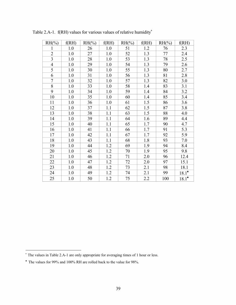
39

Table 2.A-1. f(RH) values for various values of relative humidity∗

RH(%) f(RH) RH(%) f(RH) RH(%) f(RH) RH(%) f(RH) 1 1.0 26 1.0 51 1.2 76 2.3 2 1.0 27 1.0 52 1.3 77 2.4 3 1.0 28 1.0 53 1.3 78 2.5 4 1.0 29 1.0 54 1.3 79 2.6 5 1.0 30 1.0 55 1.3 80 2.7 6 1.0 31 1.0 56 1.3 81 2.8 7 1.0 32 1.0 57 1.3 82 3.0 8 1.0 33 1.0 58 1.4 83 3.1 9 1.0 34 1.0 59 1.4 84 3.2 10 1.0 35 1.0 60 1.4 85 3.4 11 1.0 36 1.0 61 1.5 86 3.6 12 1.0 37 1.1 62 1.5 87 3.8 13 1.0 38 1.1 63 1.5 88 4.0 14 1.0 39 1.1 64 1.6 89 4.4 15 1.0 40 1.1 65 1.7 90 4.7 16 1.0 41 1.1 66 1.7 91 5.3 17 1.0 42 1.1 67 1.7 92 5.9 18 1.0 43 1.1 68 1.8 93 7.0 19 1.0 44 1.2 69 1.9 94 8.4 20 1.0 45 1.2 70 1.9 95 9.8 21 1.0 46 1.2 71 2.0 96 12.4 22 1.0 47 1.2 72 2.0 97 15.1 23 1.0 48 1.2 73 2.1 98 18.1 24 1.0 49 1.2 74 2.1 99 18.1♦

25 1.0 50 1.2 75 2.2 100 18.1♦

∗ The values in Table 2.A-1 are only appropriate for averaging times of 1 hour or less. ♦ The values for 99% and 100% RH are rolled back to the value for 98%.

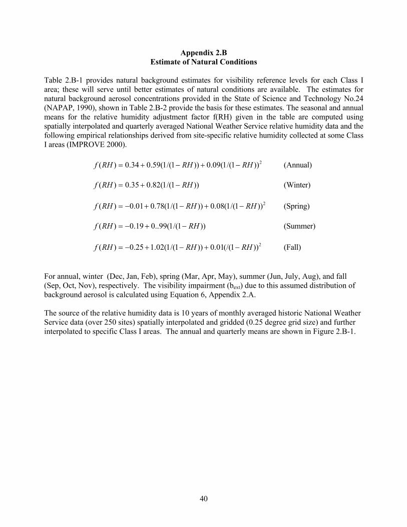
40

Appendix 2.B Estimate of Natural Conditions

Table 2.B-1 provides natural background estimates for visibility reference levels for each Class I area; these will serve until better estimates of natural conditions are available. The estimates for natural background aerosol concentrations provided in the State of Science and Technology No.24 (NAPAP, 1990), shown in Table 2.B-2 provide the basis for these estimates. The seasonal and annual means for the relative humidity adjustment factor f(RH) given in the table are computed using spatially interpolated and quarterly averaged National Weather Service relative humidity data and the following empirical relationships derived from site-specific relative humidity collected at some Class I areas (IMPROVE 2000).

2))1/(1(09.0))1/(1(59.034.0)( RHRHRHf −+−+= (Annual)

))1/(1(82.035.0)( RHRHf −+= (Winter)

2))1/(1(08.0))1/(1(78.001.0)( RHRHRHf −+−+−= (Spring)

))1/(1(99..019.0)( RHRHf −+−= (Summer)

2))1(/(01.0))1/(1(02.125.0)( RHRHRHf −+−+−= (Fall)

For annual, winter (Dec, Jan, Feb), spring (Mar, Apr, May), summer (Jun, July, Aug), and fall (Sep, Oct, Nov), respectively. The visibility impairment (bext) due to this assumed distribution of background aerosol is calculated using Equation 6, Appendix 2.A. The source of the relative humidity data is 10 years of monthly averaged historic National Weather Service data (over 250 sites) spatially interpolated and gridded (0.25 degree grid size) and further interpolated to specific Class I areas. The annual and quarterly means are shown in Figure 2.B-1.

41

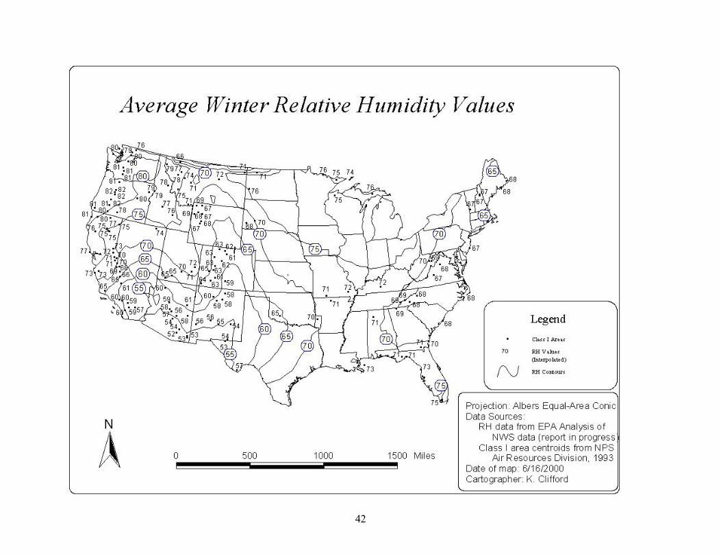
42

43

44

45

46

Site Season Components of Dry Extinction (Mm-1) f(RH)

Particle bext

w/f(RH) (Mm-1)

Reference Level

(Mm-1)

Hygro Non Hygro Rayleigh

Acadia NP Annual 0.9 8.5 10.0 3.0 11.2 21.2 Winter 0.9 8.5 10.0 2.9 11.1 21.1 Spring 0.9 8.5 10.0 2.8 11.0 21.0 Summer 0.9 8.5 10.0 3.2 11.4 21.4 Fall 0.9 8.5 10.0 3.1 11.3 21.3 Agua Tibia W Annual 0.6 4.5 10.0 2.5 6.0 16.0 Winter 0.6 4.5 10.0 2.4 5.9 15.9 Spring 0.6 4.5 10.0 2.6 6.1 16.1 Summer 0.6 4.5 10.0 2.5 6.0 16.0 Fall 0.6 4.5 10.0 2.3 5.9 15.9 Alpine Lakes W Annual 0.6 4.5 10.0 3.7 6.7 16.7 Winter 0.6 4.5 10.0 4.5 7.2 17.2 Spring 0.6 4.5 10.0 3.3 6.5 16.5 Summer 0.6 4.5 10.0 2.7 6.1 16.1 Fall 0.6 4.5 10.0 5.1 7.6 17.6 Anaconda – Pintlar W Annual 0.6 4.5 10.0 2.5 6.0 16.0 Winter 0.6 4.5 10.0 3.7 6.7 16.7 Spring 0.6 4.5 10.0 2.3 5.9 15.9 Summer 0.6 4.5 10.0 1.8 5.6 15.6 Fall 0.6 4.5 10.0 3.1 6.4 16.4 Ansel Adams W Annual 0.6 4.5 10.0 2.0 5.7 15.7 Winter 0.6 4.5 10.0 3.0 6.3 16.3 Spring 0.6 4.5 10.0 1.7 5.5 15.5 Summer 0.6 4.5 10.0 1.5 5.4 15.4 Fall 0.6 4.5 10.0 2.2 5.8 15.8 Arches NP Annual 0.6 4.5 10.0 1.9 5.6 15.6 Winter 0.6 4.5 10.0 3.3 6.5 16.5 Spring 0.6 4.5 10.0 1.5 5.4 15.4 Summer 0.6 4.5 10.0 1.4 5.3 15.3 Fall 0.6 4.5 10.0 2.3 5.9 15.9 Badlands NP (W) Annual 0.6 4.5 10.0 2.6 6.1 16.1 Winter 0.6 4.5 10.0 3.1 6.4 16.4 Spring 0.6 4.5 10.0 2.6 6.1 16.1 Summer 0.6 4.5 10.0 2.2 5.8 15.8 Fall 0.6 4.5 10.0 2.8 6.2 16.2

47


Particle bext

w/f(RH) (Mm-1)

Reference Level

(Mm-1)


Bandelier NM (W) Annual 0.6 4.5 10.0 1.8 5.6 15.6 Winter 0.6 4.5 10.0 2.3 5.9 15.9 Spring 0.6 4.5 10.0 1.5 5.4 15.4 Summer 0.6 4.5 10.0 1.7 5.5 15.5 Fall 0.6 4.5 10.0 2.0 5.7 15.7 Big Bend NP Annual 0.6 4.5 10.0 2.1 5.8 15.8 Winter 0.6 4.5 10.0 2.3 5.9 15.9 Spring 0.6 4.5 10.0 1.9 5.6 15.6 Summer 0.6 4.5 10.0 2.2 5.8 15.8 Fall 0.6 4.5 10.0 2.2 5.8 15.8 Black Canyon NP Annual 0.6 4.5 10.0 1.9 5.6 15.6 Winter 0.6 4.5 10.0 2.7 6.1 16.1 Spring 0.6 4.5 10.0 1.6 5.5 15.5 Summer 0.6 4.5 10.0 1.6 5.5 15.5 Fall 0.6 4.5 10.0 2.2 5.8 15.8 Bob Marshall W Annual 0.6 4.5 10.0 2.7 6.1 16.1 Winter 0.6 4.5 10.0 3.9 6.8 16.8 Spring 0.6 4.5 10.0 2.5 6.0 16.0 Summer 0.6 4.5 10.0 2.0 5.7 15.7 Fall 0.6 4.5 10.0 3.5 6.6 16.6 Bosque del Apache W Annual 0.6 4.5 10.0 1.7 5.5 15.5 Winter 0.6 4.5 10.0 2.2 5.8 15.8 Spring 0.6 4.5 10.0 1.3 5.3 15.3 Summer 0.6 4.5 10.0 1.7 5.5 15.5 Fall 0.6 4.5 10.0 1.8 5.6 15.6 Boundary Waters Annual 0.9 8.5 10.0 3.3 11.5 21.5 Canoe Area W Winter 0.9 8.5 10.0 3.6 11.7 21.7 Spring 0.9 8.5 10.0 2.6 10.8 20.8 Summer 0.9 8.5 10.0 3.4 11.6 21.6 Fall 0.9 8.5 10.0 3.9 12.0 22.0 Breton Island W Annual 0.9 8.5 10.0 3.8 11.9 21.9 Winter 0.9 8.5 10.0 3.4 11.6 21.6 Spring 0.9 8.5 10.0 4.0 12.1 22.1 Summer 0.9 8.5 10.0 4.1 12.2 22.2 Fall 0.9 8.5 10.0 3.6 11.7 21.7

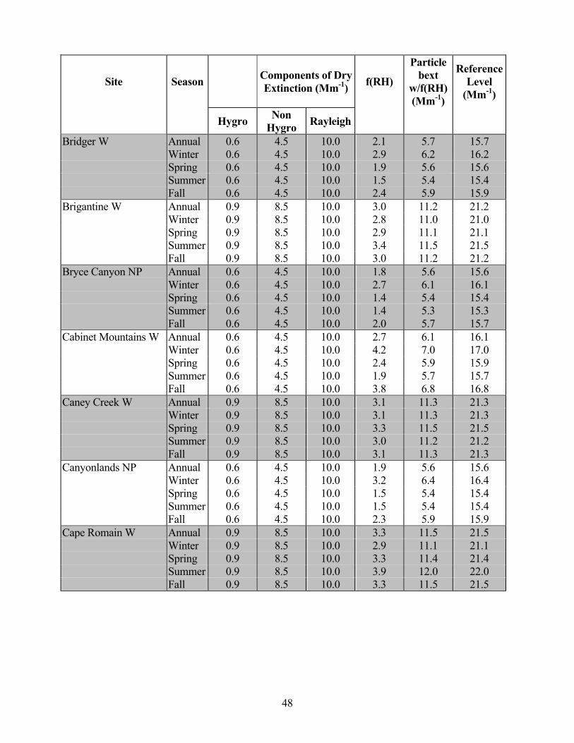
48


Particle bext

w/f(RH) (Mm-1)

Reference Level

(Mm-1)


Bridger W Annual 0.6 4.5 10.0 2.1 5.7 15.7 Winter 0.6 4.5 10.0 2.9 6.2 16.2 Spring 0.6 4.5 10.0 1.9 5.6 15.6 Summer 0.6 4.5 10.0 1.5 5.4 15.4 Fall 0.6 4.5 10.0 2.4 5.9 15.9 Brigantine W Annual 0.9 8.5 10.0 3.0 11.2 21.2 Winter 0.9 8.5 10.0 2.8 11.0 21.0 Spring 0.9 8.5 10.0 2.9 11.1 21.1 Summer 0.9 8.5 10.0 3.4 11.5 21.5 Fall 0.9 8.5 10.0 3.0 11.2 21.2 Bryce Canyon NP Annual 0.6 4.5 10.0 1.8 5.6 15.6 Winter 0.6 4.5 10.0 2.7 6.1 16.1 Spring 0.6 4.5 10.0 1.4 5.4 15.4 Summer 0.6 4.5 10.0 1.4 5.3 15.3 Fall 0.6 4.5 10.0 2.0 5.7 15.7 Cabinet Mountains W Annual 0.6 4.5 10.0 2.7 6.1 16.1 Winter 0.6 4.5 10.0 4.2 7.0 17.0 Spring 0.6 4.5 10.0 2.4 5.9 15.9 Summer 0.6 4.5 10.0 1.9 5.7 15.7 Fall 0.6 4.5 10.0 3.8 6.8 16.8 Caney Creek W Annual 0.9 8.5 10.0 3.1 11.3 21.3 Winter 0.9 8.5 10.0 3.1 11.3 21.3 Spring 0.9 8.5 10.0 3.3 11.5 21.5 Summer 0.9 8.5 10.0 3.0 11.2 21.2 Fall 0.9 8.5 10.0 3.1 11.3 21.3 Canyonlands NP Annual 0.6 4.5 10.0 1.9 5.6 15.6 Winter 0.6 4.5 10.0 3.2 6.4 16.4 Spring 0.6 4.5 10.0 1.5 5.4 15.4 Summer 0.6 4.5 10.0 1.5 5.4 15.4 Fall 0.6 4.5 10.0 2.3 5.9 15.9 Cape Romain W Annual 0.9 8.5 10.0 3.3 11.5 21.5 Winter 0.9 8.5 10.0 2.9 11.1 21.1 Spring 0.9 8.5 10.0 3.3 11.4 21.4 Summer 0.9 8.5 10.0 3.9 12.0 22.0 Fall 0.9 8.5 10.0 3.3 11.5 21.5

49


Particle bext

w/f(RH) (Mm-1)

Reference Level

(Mm-1)


Capitol Reef NP Annual 0.6 4.5 10.0 1.9 5.6 15.6 Winter 0.6 4.5 10.0 3.0 6.3 16.3 Spring 0.6 4.5 10.0 1.5 5.4 15.4 Summer 0.6 4.5 10.0 1.5 5.4 15.4 Fall 0.6 4.5 10.0 2.2 5.8 15.8 Caribou W Annual 0.6 4.5 10.0 2.3 5.9 15.9 Winter 0.6 4.5 10.0 3.6 6.6 16.6 Spring 0.6 4.5 10.0 2.0 5.7 15.7 Summer 0.6 4.5 10.0 1.7 5.5 15.5 Fall 0.6 4.5 10.0 2.7 6.1 16.1 Carlsbad Caverns NP Annual 0.6 4.5 10.0 1.8 5.6 15.6 Winter 0.6 4.5 10.0 2.1 5.8 15.8 Spring 0.6 4.5 10.0 1.5 5.4 15.4 Summer 0.6 4.5 10.0 1.9 5.6 15.6 Fall 0.6 4.5 10.0 1.8 5.6 15.6 Chassahowitzka W Annual 0.9 8.5 10.0 3.9 12.0 22.0 Winter 0.9 8.5 10.0 3.4 11.6 21.6 Spring 0.9 8.5 10.0 3.7 11.8 21.8 Summer 0.9 8.5 10.0 4.1 12.2 22.2 Fall 0.9 8.5 10.0 3.9 12.0 22.0 Chiricahua NM (W) Annual 0.6 4.5 10.0 1.6 5.4 15.4 Winter 0.6 4.5 10.0 2.1 5.8 15.8 Spring 0.6 4.5 10.0 1.2 5.2 15.2 Summer 0.6 4.5 10.0 1.5 5.4 15.4 Fall 0.6 4.5 10.0 1.6 5.5 15.5 Chiricahua W Annual 0.6 4.5 10.0 1.5 5.4 15.4 Winter 0.6 4.5 10.0 2.1 5.7 15.7 Spring 0.6 4.5 10.0 1.2 5.2 15.2 Summer 0.6 4.5 10.0 1.5 5.4 15.4 Fall 0.6 4.5 10.0 1.6 5.5 15.5 Cohutta W Annual 0.9 8.5 10.0 3.2 11.4 21.4 Winter 0.9 8.5 10.0 3.0 11.2 21.2 Spring 0.9 8.5 10.0 3.1 11.3 21.3 Summer 0.9 8.5 10.0 3.6 11.7 21.7 Fall 0.9 8.5 10.0 3.3 11.4 21.4

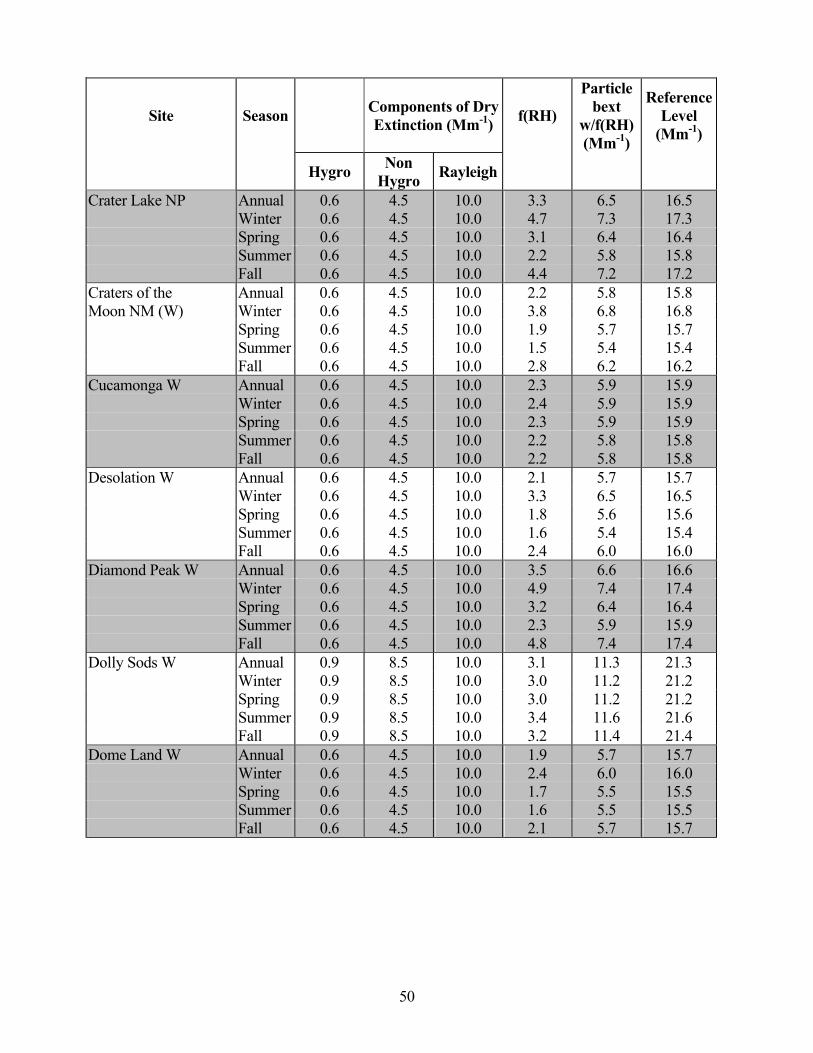
50


Particle bext

w/f(RH) (Mm-1)

Reference Level

(Mm-1)


Crater Lake NP Annual 0.6 4.5 10.0 3.3 6.5 16.5 Winter 0.6 4.5 10.0 4.7 7.3 17.3 Spring 0.6 4.5 10.0 3.1 6.4 16.4 Summer 0.6 4.5 10.0 2.2 5.8 15.8 Fall 0.6 4.5 10.0 4.4 7.2 17.2 Craters of the Annual 0.6 4.5 10.0 2.2 5.8 15.8 Moon NM (W) Winter 0.6 4.5 10.0 3.8 6.8 16.8 Spring 0.6 4.5 10.0 1.9 5.7 15.7 Summer 0.6 4.5 10.0 1.5 5.4 15.4 Fall 0.6 4.5 10.0 2.8 6.2 16.2 Cucamonga W Annual 0.6 4.5 10.0 2.3 5.9 15.9 Winter 0.6 4.5 10.0 2.4 5.9 15.9 Spring 0.6 4.5 10.0 2.3 5.9 15.9 Summer 0.6 4.5 10.0 2.2 5.8 15.8 Fall 0.6 4.5 10.0 2.2 5.8 15.8 Desolation W Annual 0.6 4.5 10.0 2.1 5.7 15.7 Winter 0.6 4.5 10.0 3.3 6.5 16.5 Spring 0.6 4.5 10.0 1.8 5.6 15.6 Summer 0.6 4.5 10.0 1.6 5.4 15.4 Fall 0.6 4.5 10.0 2.4 6.0 16.0 Diamond Peak W Annual 0.6 4.5 10.0 3.5 6.6 16.6 Winter 0.6 4.5 10.0 4.9 7.4 17.4 Spring 0.6 4.5 10.0 3.2 6.4 16.4 Summer 0.6 4.5 10.0 2.3 5.9 15.9 Fall 0.6 4.5 10.0 4.8 7.4 17.4 Dolly Sods W Annual 0.9 8.5 10.0 3.1 11.3 21.3 Winter 0.9 8.5 10.0 3.0 11.2 21.2 Spring 0.9 8.5 10.0 3.0 11.2 21.2 Summer 0.9 8.5 10.0 3.4 11.6 21.6 Fall 0.9 8.5 10.0 3.2 11.4 21.4 Dome Land W Annual 0.6 4.5 10.0 1.9 5.7 15.7 Winter 0.6 4.5 10.0 2.4 6.0 16.0 Spring 0.6 4.5 10.0 1.7 5.5 15.5 Summer 0.6 4.5 10.0 1.6 5.5 15.5 Fall 0.6 4.5 10.0 2.1 5.7 15.7

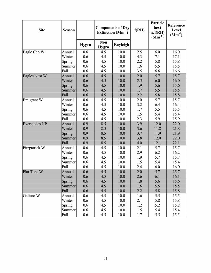
51


Particle bext

w/f(RH) (Mm-1)

Reference Level

(Mm-1)


Eagle Cap W Annual 0.6 4.5 10.0 2.5 6.0 16.0 Winter 0.6 4.5 10.0 4.3 7.1 17.1 Spring 0.6 4.5 10.0 2.2 5.8 15.8 Summer 0.6 4.5 10.0 1.6 5.5 15.5 Fall 0.6 4.5 10.0 3.5 6.6 16.6 Eagles Nest W Annual 0.6 4.5 10.0 2.0 5.7 15.7 Winter 0.6 4.5 10.0 2.5 6.0 16.0 Spring 0.6 4.5 10.0 1.9 5.6 15.6 Summer 0.6 4.5 10.0 1.7 5.5 15.5 Fall 0.6 4.5 10.0 2.2 5.8 15.8 Emigrant W Annual 0.6 4.5 10.0 2.0 5.7 15.7 Winter 0.6 4.5 10.0 3.2 6.4 16.4 Spring 0.6 4.5 10.0 1.7 5.5 15.5 Summer 0.6 4.5 10.0 1.5 5.4 15.4 Fall 0.6 4.5 10.0 2.3 5.9 15.9 Everglades NP Annual 0.9 8.5 10.0 3.9 12.0 22.0 Winter 0.9 8.5 10.0 3.6 11.8 21.8 Spring 0.9 8.5 10.0 3.7 11.9 21.9 Summer 0.9 8.5 10.0 3.8 12.0 22.0 Fall 0.9 8.5 10.0 4.0 12.1 22.1 Fitzpatrick W Annual 0.6 4.5 10.0 2.1 5.7 15.7 Winter 0.6 4.5 10.0 2.9 6.2 16.2 Spring 0.6 4.5 10.0 1.9 5.7 15.7 Summer 0.6 4.5 10.0 1.5 5.4 15.4 Fall 0.6 4.5 10.0 2.4 6.0 16.0 Flat Tops W Annual 0.6 4.5 10.0 2.0 5.7 15.7 Winter 0.6 4.5 10.0 2.6 6.1 16.1 Spring 0.6 4.5 10.0 1.8 5.6 15.6 Summer 0.6 4.5 10.0 1.6 5.5 15.5 Fall 0.6 4.5 10.0 2.2 5.8 15.8 Galiuro W Annual 0.6 4.5 10.0 1.6 5.5 15.5 Winter 0.6 4.5 10.0 2.1 5.8 15.8 Spring 0.6 4.5 10.0 1.2 5.2 15.2 Summer 0.6 4.5 10.0 1.5 5.4 15.4 Fall 0.6 4.5 10.0 1.7 5.5 15.5

52


Particle bext

w/f(RH) (Mm-1)

Reference Level

(Mm-1)


Gates of the Annual 0.6 4.5 10.0 2.4 5.9 15.9 Mountains W Winter 0.6 4.5 10.0 3.1 6.4 16.4 Spring 0.6 4.5 10.0 2.3 5.9 15.9 Summer 0.6 4.5 10.0 1.8 5.6 15.6 Fall 0.6 4.5 10.0 2.8 6.2 16.2 Gearhart Mountain W Annual 0.6 4.5 10.0 2.5 6.0 16.0 Winter 0.6 4.5 10.0 4.0 6.9 16.9 Spring 0.6 4.5 10.0 2.3 5.9 15.9 Summer 0.6 4.5 10.0 1.8 5.6 15.6 Fall 0.6 4.5 10.0 3.2 6.4 16.4 Gila W Annual 0.6 4.5 10.0 1.7 5.5 15.5 Winter 0.6 4.5 10.0 2.2 5.8 15.8 Spring 0.6 4.5 10.0 1.3 5.3 15.3 Summer 0.6 4.5 10.0 1.6 5.5 15.5 Fall 0.6 4.5 10.0 1.8 5.6 15.6 Glacier NP Annual 0.6 4.5 10.0 2.8 6.2 16.2 Winter 0.6 4.5 10.0 2.8 6.2 16.2 Spring 0.6 4.5 10.0 2.5 6.0 16.0 Summer 0.6 4.5 10.0 2.1 5.8 15.8 Fall 0.6 4.5 10.0 3.8 6.8 16.8 Glacier Peak W Annual 0.6 4.5 10.0 3.8 6.8 16.8 Winter 0.6 4.5 10.0 4.4 7.2 17.2 Spring 0.6 4.5 10.0 3.4 6.5 16.5 Summer 0.6 4.5 10.0 2.8 6.2 16.2 Fall 0.6 4.5 10.0 5.1 7.6 17.6 Goat Rocks W Annual 0.6 4.5 10.0 3.6 6.6 16.6 Winter 0.6 4.5 10.0 4.6 7.3 17.3 Spring 0.6 4.5 10.0 3.2 6.4 16.4 Summer 0.6 4.5 10.0 2.5 6.0 16.0 Fall 0.6 4.5 10.0 5.0 7.5 17.5 Grand Canyon NP Annual 0.6 4.5 10.0 1.6 5.5 15.5 Winter 0.6 4.5 10.0 2.4 5.9 15.9 Spring 0.6 4.5 10.0 1.3 5.3 15.3 Summer 0.6 4.5 10.0 1.4 5.3 15.3 Fall 0.6 4.5 10.0 1.7 5.5 15.5

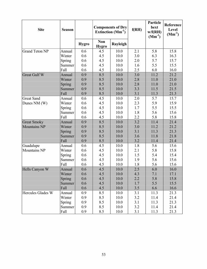
53


Particle bext

w/f(RH) (Mm-1)

Reference Level

(Mm-1)


Grand Teton NP Annual 0.6 4.5 10.0 2.1 5.8 15.8 Winter 0.6 4.5 10.0 3.0 6.3 16.3 Spring 0.6 4.5 10.0 2.0 5.7 15.7 Summer 0.6 4.5 10.0 1.6 5.5 15.5 Fall 0.6 4.5 10.0 2.5 6.0 16.0 Great Gulf W Annual 0.9 8.5 10.0 3.0 11.2 21.2 Winter 0.9 8.5 10.0 2.8 11.0 21.0 Spring 0.9 8.5 10.0 2.8 11.0 21.0 Summer 0.9 8.5 10.0 3.3 11.5 21.5 Fall 0.9 8.5 10.0 3.1 11.3 21.3 Great Sand Annual 0.6 4.5 10.0 2.0 5.7 15.7 Dunes NM (W) Winter 0.6 4.5 10.0 2.3 5.9 15.9 Spring 0.6 4.5 10.0 1.7 5.5 15.5 Summer 0.6 4.5 10.0 1.8 5.6 15.6 Fall 0.6 4.5 10.0 2.2 5.8 15.8 Great Smoky Annual 0.9 8.5 10.0 3.2 11.4 21.4 Mountains NP Winter 0.9 8.5 10.0 3.0 11.2 21.2 Spring 0.9 8.5 10.0 3.1 11.3 21.3 Summer 0.9 8.5 10.0 3.6 11.8 21.8 Fall 0.9 8.5 10.0 3.2 11.4 21.4 Guadalupe Annual 0.6 4.5 10.0 1.8 5.6 15.6 Mountains NP Winter 0.6 4.5 10.0 2.1 5.8 15.8 Spring 0.6 4.5 10.0 1.5 5.4 15.4 Summer 0.6 4.5 10.0 1.9 5.6 15.6 Fall 0.6 4.5 10.0 1.8 5.6 15.6 Hells Canyon W Annual 0.6 4.5 10.0 2.5 6.0 16.0 Winter 0.6 4.5 10.0 4.3 7.1 17.1 Spring 0.6 4.5 10.0 2.2 5.8 15.8 Summer 0.6 4.5 10.0 1.7 5.5 15.5 Fall 0.6 4.5 10.0 3.5 6.6 16.6 Hercules Glades W Annual 0.9 8.5 10.0 3.1 11.3 21.3 Winter 0.9 8.5 10.0 3.2 11.4 21.4 Spring 0.9 8.5 10.0 3.1 11.3 21.3 Summer 0.9 8.5 10.0 3.2 11.4 21.4 Fall 0.9 8.5 10.0 3.1 11.3 21.3

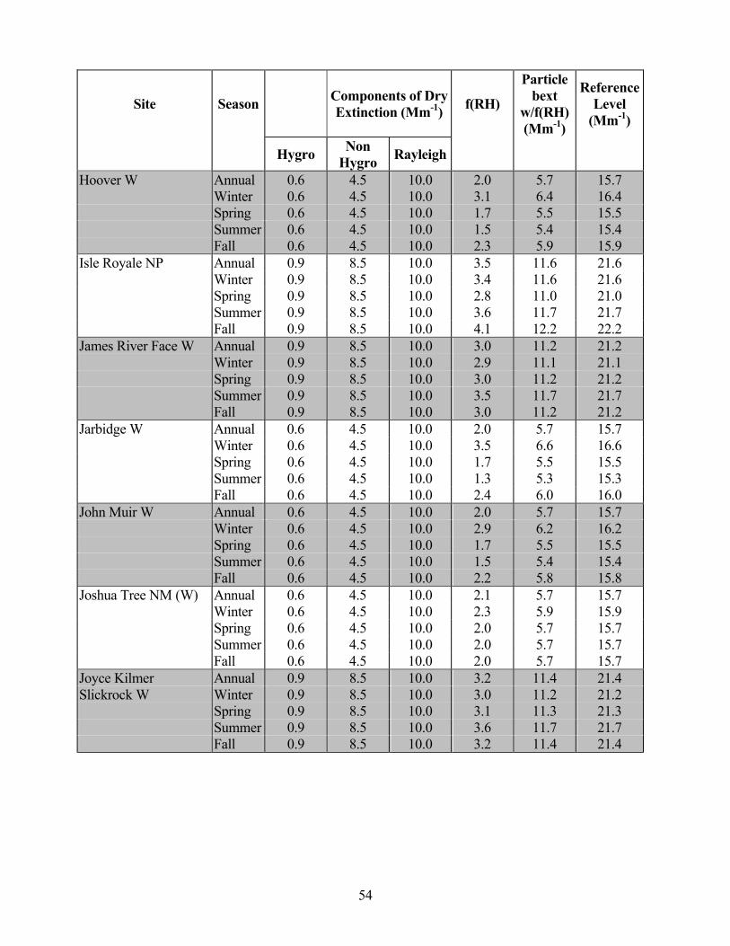
54


Particle bext

w/f(RH) (Mm-1)

Reference Level

(Mm-1)


Hoover W Annual 0.6 4.5 10.0 2.0 5.7 15.7 Winter 0.6 4.5 10.0 3.1 6.4 16.4 Spring 0.6 4.5 10.0 1.7 5.5 15.5 Summer 0.6 4.5 10.0 1.5 5.4 15.4 Fall 0.6 4.5 10.0 2.3 5.9 15.9 Isle Royale NP Annual 0.9 8.5 10.0 3.5 11.6 21.6 Winter 0.9 8.5 10.0 3.4 11.6 21.6 Spring 0.9 8.5 10.0 2.8 11.0 21.0 Summer 0.9 8.5 10.0 3.6 11.7 21.7 Fall 0.9 8.5 10.0 4.1 12.2 22.2 James River Face W Annual 0.9 8.5 10.0 3.0 11.2 21.2 Winter 0.9 8.5 10.0 2.9 11.1 21.1 Spring 0.9 8.5 10.0 3.0 11.2 21.2 Summer 0.9 8.5 10.0 3.5 11.7 21.7 Fall 0.9 8.5 10.0 3.0 11.2 21.2 Jarbidge W Annual 0.6 4.5 10.0 2.0 5.7 15.7 Winter 0.6 4.5 10.0 3.5 6.6 16.6 Spring 0.6 4.5 10.0 1.7 5.5 15.5 Summer 0.6 4.5 10.0 1.3 5.3 15.3 Fall 0.6 4.5 10.0 2.4 6.0 16.0 John Muir W Annual 0.6 4.5 10.0 2.0 5.7 15.7 Winter 0.6 4.5 10.0 2.9 6.2 16.2 Spring 0.6 4.5 10.0 1.7 5.5 15.5 Summer 0.6 4.5 10.0 1.5 5.4 15.4 Fall 0.6 4.5 10.0 2.2 5.8 15.8 Joshua Tree NM (W) Annual 0.6 4.5 10.0 2.1 5.7 15.7 Winter 0.6 4.5 10.0 2.3 5.9 15.9 Spring 0.6 4.5 10.0 2.0 5.7 15.7 Summer 0.6 4.5 10.0 2.0 5.7 15.7 Fall 0.6 4.5 10.0 2.0 5.7 15.7 Joyce Kilmer Annual 0.9 8.5 10.0 3.2 11.4 21.4 Slickrock W Winter 0.9 8.5 10.0 3.0 11.2 21.2 Spring 0.9 8.5 10.0 3.1 11.3 21.3 Summer 0.9 8.5 10.0 3.6 11.7 21.7 Fall 0.9 8.5 10.0 3.2 11.4 21.4

55


Particle bext

w/f(RH) (Mm-1)

Reference Level

(Mm-1)


Kaiser W Annual 0.6 4.5 10.0 2.0 5.7 15.7 Winter 0.6 4.5 10.0 3.0 6.3 16.3 Spring 0.6 4.5 10.0 1.7 5.5 15.5 Summer 0.6 4.5 10.0 1.6 5.5 15.5 Fall 0.6 4.5 10.0 2.3 5.9 15.9 Kalmiopsis W Annual 0.6 4.5 10.0 3.4 6.5 16.5 Winter 0.6 4.5 10.0 4.7 7.3 17.3 Spring 0.6 4.5 10.0 3.2 6.4 16.4 Summer 0.6 4.5 10.0 2.3 5.9 15.9 Fall 0.6 4.5 10.0 4.4 7.2 17.2 Kings Canyon NP Annual 0.6 4.5 10.0 2.0 5.7 15.7 Winter 0.6 4.5 10.0 2.8 6.2 16.2 Spring 0.6 4.5 10.0 1.7 5.5 15.5 Summer 0.6 4.5 10.0 1.6 5.5 15.5 Fall 0.6 4.5 10.0 2.2 5.8 15.8 La Garita W p 0.6 4.5 10.0 1.9 5.6 15.6 Winter 0.6 4.5 10.0 2.5 6.0 16.0 Spring 0.6 4.5 10.0 1.6 5.5 15.5 Summer 0.6 4.5 10.0 1.7 5.5 15.5 Fall 0.6 4.5 10.0 2.2 5.8 15.8 Lassen Volcanic NP Annual 0.6 4.5 10.0 2.3 5.9 15.9 Winter 0.6 4.5 10.0 3.6 6.7 16.7 Spring 0.6 4.5 10.0 2.1 5.7 15.7 Summer 0.6 4.5 10.0 1.7 5.5 15.5 Fall 0.6 4.5 10.0 2.7 6.1 16.1 Lava Beds NM (W) Annual 0.6 4.5 10.0 2.5 6.0 16.0 Winter 0.6 4.5 10.0 3.9 6.9 16.9 Spring 0.6 4.5 10.0 2.2 5.8 15.8 Summer 0.6 4.5 10.0 1.7 5.5 15.5 Fall 0.6 4.5 10.0 3.1 6.4 16.4 Linville Gorge W Annual 0.9 8.5 10.0 3.2 11.3 21.3 Winter 0.9 8.5 10.0 2.9 11.1 21.1 Spring 0.9 8.5 10.0 3.1 11.3 21.3 Summer 0.9 8.5 10.0 3.7 11.8 21.8 Fall 0.9 8.5 10.0 3.1 11.3 21.3

56


Particle bext

w/f(RH) (Mm-1)

Reference Level

(Mm-1)


Lostwood W Annual 0.6 4.5 10.0 2.9 6.2 16.2 Winter 0.6 4.5 10.0 3.2 6.4 16.4 Spring 0.6 4.5 10.0 2.4 5.9 15.9 Summer 0.6 4.5 10.0 2.3 5.9 15.9 Fall 0.6 4.5 10.0 3.5 6.6 16.6 Lye Brook W Annual 0.9 8.5 10.0 3.0 11.2 21.2 Winter 0.9 8.5 10.0 2.9 11.1 21.1 Spring 0.9 8.5 10.0 2.8 11.0 21.0 Summer 0.9 8.5 10.0 3.3 11.4 21.4 Fall 0.9 8.5 10.0 3.1 11.3 21.3 Mammoth Cave NP Annual 0.9 8.5 10.0 3.2 11.4 21.4 Winter 0.9 8.5 10.0 3.3 11.5 21.5 Spring 0.9 8.5 10.0 3.1 11.3 21.3 Summer 0.9 8.5 10.0 3.4 11.6 21.6 Fall 0.9 8.5 10.0 3.3 11.5 21.5 Marble Mountain W Annual 0.6 4.5 10.0 3.1 6.3 16.3 Winter 0.6 4.5 10.0 4.4 7.1 17.1 Spring 0.6 4.5 10.0 2.9 6.2 16.2 Summer 0.6 4.5 10.0 2.2 5.8 15.8 Fall 0.6 4.5 10.0 3.8 6.8 16.8 Maroon Bells Annual 0.6 4.5 10.0 1.9 5.7 15.7 Snowmass W Winter 0.6 4.5 10.0 2.6 6.0 16.0 Spring 0.6 4.5 10.0 1.7 5.5 15.5 Summer 0.6 4.5 10.0 1.6 5.5 15.5 Fall 0.6 4.5 10.0 2.1 5.8 15.8 Mazatzal W Annual 0.6 4.5 10.0 1.6 5.5 15.5 Winter 0.6 4.5 10.0 2.2 5.8 15.8 Spring 0.6 4.5 10.0 1.3 5.3 15.3 Summer 0.6 4.5 10.0 1.5 5.4 15.4 Fall 0.6 4.5 10.0 1.7 5.5 15.5 Medicine Lake W Annual 0.6 4.5 10.0 2.8 6.2 16.2 Winter 0.6 4.5 10.0 3.2 6.4 16.4 Spring 0.6 4.5 10.0 2.4 5.9 15.9 Summer 0.6 4.5 10.0 2.2 5.8 15.8 Fall 0.6 4.5 10.0 3.5 6.6 16.6

57


Particle bext

w/f(RH) (Mm-1)

Reference Level

(Mm-1)


Mesa Verde NP Annual 0.6 4.5 10.0 1.9 5.6 15.6 Winter 0.6 4.5 10.0 2.6 6.1 16.1 Spring 0.6 4.5 10.0 1.5 5.4 15.4 Summer 0.6 4.5 10.0 1.7 5.5 15.5 Fall 0.6 4.5 10.0 2.1 5.8 15.8 Mingo W Annual 0.9 8.5 10.0 3.2 11.3 21.3 Winter 0.9 8.5 10.0 3.3 11.4 21.4 Spring 0.9 8.5 10.0 3.0 11.2 21.2 Summer 0.9 8.5 10.0 3.3 11.4 21.4 Fall 0.9 8.5 10.0 3.2 11.4 21.4 Mission Mountains W Annual 0.6 4.5 10.0 2.7 6.1 16.1 Winter 0.6 4.5 10.0 4.0 6.9 16.9 Spring 0.6 4.5 10.0 2.5 6.0 16.0 Summer 0.6 4.5 10.0 2.0 5.7 15.7 Fall 0.6 4.5 10.0 3.6 6.7 16.7 Mokelumne W Annual 0.6 4.5 10.0 2.0 5.7 15.7 Winter 0.6 4.5 10.0 3.3 6.5 16.5 Spring 0.6 4.5 10.0 1.7 5.5 15.5 Summer 0.6 4.5 10.0 1.5 5.4 15.4 Fall 0.6 4.5 10.0 2.4 5.9 15.9 Moosehorn W Annual 0.9 8.5 10.0 3.0 11.2 21.2 Winter 0.9 8.5 10.0 2.9 11.2 21.2 Spring 0.9 8.5 10.0 2.8 11.0 21.0 Summer 0.9 8.5 10.0 3.2 11.4 21.4 Fall 0.9 8.5 10.0 3.2 11.4 21.4 Mount Adams W Annual 0.6 4.5 10.0 3.6 6.7 16.7 Winter 0.6 4.5 10.0 4.7 7.3 17.3 Spring 0.6 4.5 10.0 3.2 6.4 16.4 Summer 0.6 4.5 10.0 2.5 6.0 16.0 Fall 0.6 4.5 10.0 5.0 7.5 17.5 Mount Baldy W Annual 0.6 4.5 10.0 1.7 5.5 15.5 Winter 0.6 4.5 10.0 2.3 5.9 15.9 Spring 0.6 4.5 10.0 1.3 5.3 15.3 Summer 0.6 4.5 10.0 1.6 5.5 15.5 Fall 0.6 4.5 10.0 1.8 5.6 15.6

58


Particle bext

w/f(RH) (Mm-1)

Reference Level

(Mm-1)


Mount Hood W Annual 0.6 4.5 10.0 3.7 6.7 16.7 Winter 0.6 4.5 10.0 4.7 7.3 17.3 Spring 0.6 4.5 10.0 3.4 6.5 16.5 Summer 0.6 4.5 10.0 2.6 6.1 16.1 Fall 0.6 4.5 10.0 5.2 7.6 17.6 Mount Jefferson W Annual 0.6 4.5 10.0 3.7 6.7 16.7 Winter 0.6 4.5 10.0 4.8 7.4 17.4 Spring 0.6 4.5 10.0 3.4 6.5 16.5 Summer 0.6 4.5 10.0 2.5 6.0 16.0 Fall 0.6 4.5 10.0 5.2 7.6 17.6 Mount Rainier NP Annual 0.6 4.5 10.0 3.8 6.8 16.8 Winter 0.6 4.5 10.0 4.6 7.3 17.3 Spring 0.6 4.5 10.0 3.4 6.5 16.5 Summer 0.6 4.5 10.0 2.7 6.1 16.1 Fall 0.6 4.5 10.0 5.2 7.6 17.6 Mount Washington W Annual 0.6 4.5 10.0 3.7 6.7 16.7 Winter 0.6 4.5 10.0 4.8 7.4 17.4 Spring 0.6 4.5 10.0 3.4 6.5 16.5 Summer 0.6 4.5 10.0 2.5 6.0 16.0 Fall 0.6 4.5 10.0 5.1 7.6 17.6 Mount Zirkel W Annual 0.6 4.5 10.0 2.0 5.7 15.7 Winter 0.6 4.5 10.0 2.5 6.0 16.0 Spring 0.6 4.5 10.0 1.9 5.6 15.6 Summer 0.6 4.5 10.0 1.7 5.5 15.5 Fall 0.6 4.5 10.0 2.2 5.8 15.8 Mountain Lakes W Annual 0.6 4.5 10.0 2.8 6.2 16.2 Winter 0.6 4.5 10.0 4.4 7.2 17.2 Spring 0.6 4.5 10.0 2.6 6.1 16.1 Summer 0.6 4.5 10.0 1.9 5.7 15.7 Fall 0.6 4.5 10.0 3.8 6.8 16.8 North Absoraka W Annual 0.6 4.5 10.0 2.2 5.8 15.8 Winter 0.6 4.5 10.0 2.9 6.2 16.2 Spring 0.6 4.5 10.0 2.1 5.8 15.8 Summer 0.6 4.5 10.0 1.7 5.5 15.5 Fall 0.6 4.5 10.0 2.5 6.0 16.0

59


Particle bext

w/f(RH) (Mm-1)

Reference Level

(Mm-1)


North Cascades NP Annual 0.6 4.5 10.0 3.8 6.8 16.8 Winter 0.6 4.5 10.0 4.2 7.0 17.0 Spring 0.6 4.5 10.0 3.4 6.5 16.5 Summer 0.6 4.5 10.0 2.8 6.2 16.2 Fall 0.6 4.5 10.0 5.1 7.6 17.6 Okefenokee W Annual 0.9 8.5 10.0 3.5 11.7 21.7 Winter 0.9 8.5 10.0 3.2 11.3 21.3 Spring 0.9 8.5 10.0 3.4 11.5 21.5 Summer 0.9 8.5 10.0 3.9 12.0 22.0 Fall 0.9 8.5 10.0 3.6 11.7 21.7 Olympic NP Annual 0.6 4.5 10.0 4.5 7.2 17.2 Winter 0.6 4.5 10.0 4.4 7.2 17.2 Spring 0.6 4.5 10.0 4.1 7.0 17.0 Summer 0.6 4.5 10.0 3.4 6.5 16.5 Fall 0.6 4.5 10.0 5.8 8.0 18.0 Otter Creek W Annual 0.9 8.5 10.0 3.2 11.3 21.3 Winter 0.9 8.5 10.0 3.0 11.2 21.2 Spring 0.9 8.5 10.0 3.0 11.2 21.2 Summer 0.9 8.5 10.0 3.5 11.6 21.6 Fall 0.9 8.5 10.0 3.2 11.4 21.4 Pasayten W Annual 0.6 4.5 10.0 3.7 6.7 16.7 Winter 0.6 4.5 10.0 3.8 6.8 16.8 Spring 0.6 4.5 10.0 3.3 6.5 16.5 Summer 0.6 4.5 10.0 2.7 6.1 16.1 Fall 0.6 4.5 10.0 5.0 7.5 17.5 Pecos W Annual 0.6 4.5 10.0 1.8 5.6 15.6 Winter 0.6 4.5 10.0 2.3 5.9 15.9 Spring 0.6 4.5 10.0 1.5 5.4 15.4 Summer 0.6 4.5 10.0 1.8 5.6 15.6 Fall 0.6 4.5 10.0 2.0 5.7 15.7 Petrified Forest NP Annual 0.6 4.5 10.0 1.7 5.5 15.5 Winter 0.6 4.5 10.0 2.5 6.0 16.0 Spring 0.6 4.5 10.0 1.3 5.3 15.3 Summer 0.6 4.5 10.0 1.6 5.5 15.5 Fall 0.6 4.5 10.0 1.9 5.6 15.6

60


Particle bext

w/f(RH) (Mm-1)

Reference Level

(Mm-1)


Pine Mountain W Annual 0.6 4.5 10.0 1.6 5.5 15.5 Winter 0.6 4.5 10.0 2.3 5.9 15.9 Spring 0.6 4.5 10.0 1.3 5.3 15.3 Summer 0.6 4.5 10.0 1.5 5.4 15.4 Fall 0.6 4.5 10.0 1.7 5.5 15.5 Pinnacles NM (W) Annual 0.6 4.5 10.0 2.4 5.9 15.9 Winter 0.6 4.5 10.0 3.4 6.5 16.5 Spring 0.6 4.5 10.0 2.1 5.8 15.8 Summer 0.6 4.5 10.0 2.0 5.7 15.7 Fall 0.6 4.5 10.0 2.7 6.1 16.1 Point Reyes NS (W) Annual 0.6 4.5 10.0 3.0 6.3 16.3 Winter 0.6 4.5 10.0 3.9 6.9 16.9 Spring 0.6 4.5 10.0 2.7 6.1 16.1 Summer 0.6 4.5 10.0 2.5 6.0 16.0 Fall 0.6 4.5 10.0 3.1 6.4 16.4 Presidential Range Annual 0.9 8.5 10.0 3.0 11.2 21.2 Dry River W Winter 0.9 8.5 10.0 2.8 11.0 21.0 Spring 0.9 8.5 10.0 2.8 11.0 21.0 Summer 0.9 8.5 10.0 3.3 11.5 21.5 Fall 0.9 8.5 10.0 3.1 11.3 21.3 Rawah W Annual 0.6 4.5 10.0 2.1 5.7 15.7 Winter 0.6 4.5 10.0 2.5 6.0 16.0 Spring 0.6 4.5 10.0 2.0 5.7 15.7 Summer 0.6 4.5 10.0 1.8 5.6 15.6 Fall 0.6 4.5 10.0 2.2 5.8 15.8 Red Rock Lakes W Annual 0.6 4.5 10.0 2.2 5.8 15.8 Winter 0.6 4.5 10.0 3.2 6.4 16.4 Spring 0.6 4.5 10.0 2.1 5.8 15.8 Summer 0.6 4.5 10.0 1.7 5.5 15.5 Fall 0.6 4.5 10.0 2.7 6.1 16.1 Redwood NP Annual 0.6 4.5 10.0 4.2 7.0 17.0 Winter 0.6 4.5 10.0 4.6 7.3 17.3 Spring 0.6 4.5 10.0 4.3 7.1 17.1 Summer 0.6 4.5 10.0 3.2 6.4 16.4 Fall 0.6 4.5 10.0 4.6 7.3 17.3

61


Particle bext

w/f(RH) (Mm-1)

Reference Level

(Mm-1)


Rocky Mountain NP Annual 0.6 4.5 10.0 2.1 5.7 15.7 Winter 0.6 4.5 10.0 2.5 6.0 16.0 Spring 0.6 4.5 10.0 2.0 5.7 15.7 Summer 0.6 4.5 10.0 1.8 5.6 15.6 Fall 0.6 4.5 10.0 2.2 5.8 15.8 Saguaro NP Annual 0.6 4.5 10.0 1.6 5.4 15.4 Winter 0.6 4.5 10.0 2.1 5.7 15.7 Spring 0.6 4.5 10.0 1.2 5.2 15.2 Summer 0.6 4.5 10.0 1.5 5.4 15.4 Fall 0.6 4.5 10.0 1.6 5.5 15.5 Salt Creek W Annual 0.6 4.5 10.0 1.8 5.6 15.6 Winter 0.6 4.5 10.0 2.1 5.8 15.8 Spring 0.6 4.5 10.0 1.5 5.4 15.4 Summer 0.6 4.5 10.0 1.9 5.6 15.6 Fall 0.6 4.5 10.0 1.8 5.6 15.6 San Gabriel W Annual 0.6 4.5 10.0 2.4 5.9 15.9 Winter 0.6 4.5 10.0 2.4 5.9 15.9 Spring 0.6 4.5 10.0 2.4 6.0 16.0 Summer 0.6 4.5 10.0 2.4 5.9 15.9 Fall 0.6 4.5 10.0 2.2 5.8 15.8 San Gorgonio W Annual 0.6 4.5 10.0 2.2 5.8 15.8 Winter 0.6 4.5 10.0 2.3 5.9 15.9 Spring 0.6 4.5 10.0 2.2 5.8 15.8 Summer 0.6 4.5 10.0 2.1 5.8 15.8 Fall 0.6 4.5 10.0 2.1 5.8 15.8 San Jacinto W Annual 0.6 4.5 10.0 2.3 5.9 15.9 Winter 0.6 4.5 10.0 2.3 5.9 15.9 Spring 0.6 4.5 10.0 2.3 5.9 15.9 Summer 0.6 4.5 10.0 2.2 5.8 15.8 Fall 0.6 4.5 10.0 2.1 5.8 15.8 San Pedro Parks W Annual 0.6 4.5 10.0 1.8 5.6 15.6 Winter 0.6 4.5 10.0 2.4 6.0 16.0 Spring 0.6 4.5 10.0 1.5 5.4 15.4 Summer 0.6 4.5 10.0 1.7 5.5 15.5 Fall 0.6 4.5 10.0 2.0 5.7 15.7

62


Particle bext

w/f(RH) (Mm-1)

Reference Level

(Mm-1)


San Rafael W Annual 0.6 4.5 10.0 2.6 6.1 16.1 Winter 0.6 4.5 10.0 2.7 6.1 16.1 Spring 0.6 4.5 10.0 2.6 6.0 16.0 Summer 0.6 4.5 10.0 2.5 6.0 16.0 Fall 0.6 4.5 10.0 2.5 6.0 16.0 Sawtooth W Annual 0.6 4.5 10.0 2.2 5.8 15.8 Winter 0.6 4.5 10.0 4.0 6.9 16.9 Spring 0.6 4.5 10.0 2.0 5.7 15.7 Summer 0.6 4.5 10.0 1.5 5.4 15.4 Fall 0.6 4.5 10.0 2.9 6.2 16.2 Scapegoat W Annual 0.6 4.5 10.0 2.5 6.0 16.0 Winter 0.6 4.5 10.0 3.5 6.6 16.6 Spring 0.6 4.5 10.0 2.4 5.9 15.9 Summer 0.6 4.5 10.0 1.9 5.6 15.6 Fall 0.6 4.5 10.0 3.1 6.3 16.3 Selway – Bitterroot W Annual 0.6 4.5 10.0 2.6 6.0 16.0 Winter 0.6 4.5 10.0 4.0 6.9 16.9 Spring 0.6 4.5 10.0 2.3 5.9 15.9 Summer 0.6 4.5 10.0 1.8 5.6 15.6 Fall 0.6 4.5 10.0 3.4 6.5 16.5 Seney W Annual 0.9 8.5 10.0 3.6 11.8 21.8 Winter 0.9 8.5 10.0 3.7 11.8 21.8 Spring 0.9 8.5 10.0 2.9 11.1 21.1 Summer 0.9 8.5 10.0 3.6 11.7 21.7 Fall 0.9 8.5 10.0 4.2 12.3 22.3 Sequoia NP Annual 0.6 4.5 10.0 2.0 5.7 15.7 Winter 0.6 4.5 10.0 2.7 6.1 16.1 Spring 0.6 4.5 10.0 1.8 5.6 15.6 Summer 0.6 4.5 10.0 1.6 5.5 15.5 Fall 0.6 4.5 10.0 2.1 5.8 15.8 Shenandoah NP Annual 0.9 8.5 10.0 3.0 11.2 21.2 Winter 0.9 8.5 10.0 2.9 11.1 21.1 Spring 0.9 8.5 10.0 2.9 11.1 21.1 Summer 0.9 8.5 10.0 3.4 11.6 21.6 Fall 0.9 8.5 10.0 3.1 11.3 21.3

63


Particle bext

w/f(RH) (Mm-1)

Reference Level

(Mm-1)


Shining Rock W Annual 0.9 8.5 10.0 3.2 11.4 21.4 Winter 0.9 8.5 10.0 2.9 11.1 21.1 Spring 0.9 8.5 10.0 3.1 11.3 21.3 Summer 0.9 8.5 10.0 3.7 11.9 21.9 Fall 0.9 8.5 10.0 3.2 11.3 21.3 Sierra Ancha W Annual 0.6 4.5 10.0 1.6 5.5 15.5 Winter 0.6 4.5 10.0 2.2 5.8 15.8 Spring 0.6 4.5 10.0 1.3 5.3 15.3 Summer 0.6 4.5 10.0 1.5 5.4 15.4 Fall 0.6 4.5 10.0 1.7 5.5 15.5 Sipsey W Annual 0.9 8.5 10.0 3.3 11.5 21.5 Winter 0.9 8.5 10.0 3.2 11.4 21.4 Spring 0.9 8.5 10.0 3.3 11.4 21.4 Summer 0.9 8.5 10.0 3.5 11.7 21.7 Fall 0.9 8.5 10.0 3.3 11.5 21.5 South Warner W Annual 0.6 4.5 10.0 2.1 5.8 15.8 Winter 0.6 4.5 10.0 3.6 6.7 16.7 Spring 0.6 4.5 10.0 1.9 5.6 15.6 Summer 0.6 4.5 10.0 1.5 5.4 15.4 Fall 0.6 4.5 10.0 2.6 6.1 16.1 St. Marks W Annual 0.9 8.5 10.0 3.6 11.8 21.8 Winter 0.9 8.5 10.0 3.2 11.4 21.4 Spring 0.9 8.5 10.0 3.5 11.7 21.7 Summer 0.9 8.5 10.0 4.0 12.1 22.1 Fall 0.9 8.5 10.0 3.6 11.8 21.8 Strawberry Mountain W

Annual 0.6 4.5 10.0 2.6 6.1 16.1

Winter 0.6 4.5 10.0 4.4 7.1 17.1 Spring 0.6 4.5 10.0 2.4 5.9 15.9 Summer 0.6 4.5 10.0 1.8 5.6 15.6 Fall 0.6 4.5 10.0 3.7 6.7 16.7 Superstition W Annual 0.6 4.5 10.0 1.6 5.4 15.4 Winter 0.6 4.5 10.0 2.1 5.8 15.8 Spring 0.6 4.5 10.0 1.2 5.2 15.2 Summer 0.6 4.5 10.0 1.5 5.4 15.4 Fall 0.6 4.5 10.0 1.6 5.5 15.5

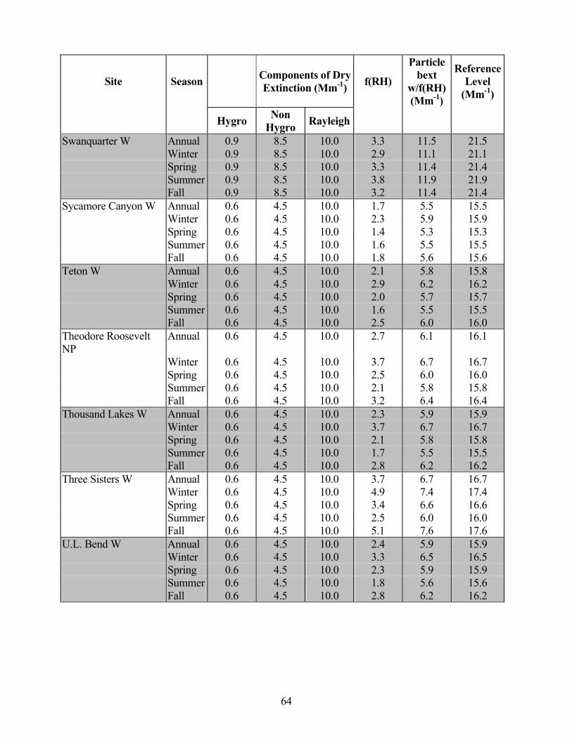
64


Particle bext

w/f(RH) (Mm-1)

Reference Level

(Mm-1)


Swanquarter W Annual 0.9 8.5 10.0 3.3 11.5 21.5 Winter 0.9 8.5 10.0 2.9 11.1 21.1 Spring 0.9 8.5 10.0 3.3 11.4 21.4 Summer 0.9 8.5 10.0 3.8 11.9 21.9 Fall 0.9 8.5 10.0 3.2 11.4 21.4 Sycamore Canyon W Annual 0.6 4.5 10.0 1.7 5.5 15.5 Winter 0.6 4.5 10.0 2.3 5.9 15.9 Spring 0.6 4.5 10.0 1.4 5.3 15.3 Summer 0.6 4.5 10.0 1.6 5.5 15.5 Fall 0.6 4.5 10.0 1.8 5.6 15.6 Teton W Annual 0.6 4.5 10.0 2.1 5.8 15.8 Winter 0.6 4.5 10.0 2.9 6.2 16.2 Spring 0.6 4.5 10.0 2.0 5.7 15.7 Summer 0.6 4.5 10.0 1.6 5.5 15.5 Fall 0.6 4.5 10.0 2.5 6.0 16.0 Theodore Roosevelt NP

Annual 0.6 4.5 10.0 2.7 6.1 16.1

Winter 0.6 4.5 10.0 3.7 6.7 16.7 Spring 0.6 4.5 10.0 2.5 6.0 16.0 Summer 0.6 4.5 10.0 2.1 5.8 15.8 Fall 0.6 4.5 10.0 3.2 6.4 16.4 Thousand Lakes W Annual 0.6 4.5 10.0 2.3 5.9 15.9 Winter 0.6 4.5 10.0 3.7 6.7 16.7 Spring 0.6 4.5 10.0 2.1 5.8 15.8 Summer 0.6 4.5 10.0 1.7 5.5 15.5 Fall 0.6 4.5 10.0 2.8 6.2 16.2 Three Sisters W Annual 0.6 4.5 10.0 3.7 6.7 16.7 Winter 0.6 4.5 10.0 4.9 7.4 17.4 Spring 0.6 4.5 10.0 3.4 6.6 16.6 Summer 0.6 4.5 10.0 2.5 6.0 16.0 Fall 0.6 4.5 10.0 5.1 7.6 17.6 U.L. Bend W Annual 0.6 4.5 10.0 2.4 5.9 15.9 Winter 0.6 4.5 10.0 3.3 6.5 16.5 Spring 0.6 4.5 10.0 2.3 5.9 15.9 Summer 0.6 4.5 10.0 1.8 5.6 15.6 Fall 0.6 4.5 10.0 2.8 6.2 16.2

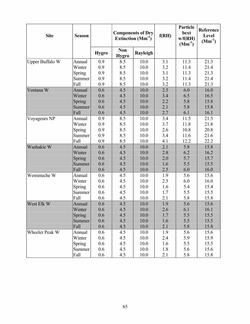
65


Particle bext

w/f(RH) (Mm-1)

Reference Level

(Mm-1)


Upper Buffalo W Annual 0.9 8.5 10.0 3.1 11.3 21.3 Winter 0.9 8.5 10.0 3.2 11.4 21.4 Spring 0.9 8.5 10.0 3.1 11.3 21.3 Summer 0.9 8.5 10.0 3.2 11.4 21.4 Fall 0.9 8.5 10.0 3.2 11.3 21.3 Ventana W Annual 0.6 4.5 10.0 2.5 6.0 16.0 Winter 0.6 4.5 10.0 3.4 6.5 16.5 Spring 0.6 4.5 10.0 2.2 5.8 15.8 Summer 0.6 4.5 10.0 2.1 5.8 15.8 Fall 0.6 4.5 10.0 2.7 6.1 16.1 Voyageurs NP Annual 0.9 8.5 10.0 3.4 11.5 21.5 Winter 0.9 8.5 10.0 3.7 11.8 21.8 Spring 0.9 8.5 10.0 2.6 10.8 20.8 Summer 0.9 8.5 10.0 3.4 11.6 21.6 Fall 0.9 8.5 10.0 4.1 12.2 22.2 Washakie W Annual 0.6 4.5 10.0 2.1 5.8 15.8 Winter 0.6 4.5 10.0 2.8 6.2 16.2 Spring 0.6 4.5 10.0 2.0 5.7 15.7 Summer 0.6 4.5 10.0 1.6 5.5 15.5 Fall 0.6 4.5 10.0 2.5 6.0 16.0 Weminuche W Annual 0.6 4.5 10.0 1.9 5.6 15.6 Winter 0.6 4.5 10.0 2.5 6.0 16.0 Spring 0.6 4.5 10.0 1.6 5.4 15.4 Summer 0.6 4.5 10.0 1.7 5.5 15.5 Fall 0.6 4.5 10.0 2.1 5.8 15.8 West Elk W Annual 0.6 4.5 10.0 1.9 5.6 15.6 Winter 0.6 4.5 10.0 2.6 6.1 16.1 Spring 0.6 4.5 10.0 1.7 5.5 15.5 Summer 0.6 4.5 10.0 1.6 5.5 15.5 Fall 0.6 4.5 10.0 2.1 5.8 15.8 Wheeler Peak W Annual 0.6 4.5 10.0 1.9 5.6 15.6 Winter 0.6 4.5 10.0 2.4 5.9 15.9 Spring 0.6 4.5 10.0 1.6 5.5 15.5 Summer 0.6 4.5 10.0 1.8 5.6 15.6 Fall 0.6 4.5 10.0 2.1 5.8 15.8

66


Particle bext

w/f(RH) (Mm-1)

Reference Level

(Mm-1)


White Mountain W Annual 0.6 4.5 10.0 1.8 5.6 15.6 Winter 0.6 4.5 10.0 2.2 5.8 15.8 Spring 0.6 4.5 10.0 1.4 5.4 15.4 Summer 0.6 4.5 10.0 1.8 5.6 15.6 Fall 0.6 4.5 10.0 1.8 5.6 15.6 Wichita Mountain W Annual 0.6 4.5 10.0 2.6 6.1 16.1 Winter 0.6 4.5 10.0 2.7 6.1 16.1 Spring 0.6 4.5 10.0 2.8 6.2 16.2 Summer 0.6 4.5 10.0 2.5 6.0 16.0 Fall 0.6 4.5 10.0 2.6 6.1 16.1 Wind Cave NP Annual 0.6 4.5 10.0 2.5 6.0 16.0 Winter 0.6 4.5 10.0 2.9 6.2 16.2 Spring 0.6 4.5 10.0 2.5 6.0 16.0 Summer 0.6 4.5 10.0 2.1 5.7 15.7 Fall 0.6 4.5 10.0 2.6 6.1 16.1 Wolf Island W Annual 0.9 8.5 10.0 3.5 11.6 21.6 Winter 0.9 8.5 10.0 3.1 11.3 21.3 Spring 0.9 8.5 10.0 3.3 11.5 21.5 Summer 0.9 8.5 10.0 3.9 12.0 22.0 Fall 0.9 8.5 10.0 3.6 11.7 21.7 Yellowstone NP Annual 0.6 4.5 10.0 2.2 5.8 15.8 Winter 0.6 4.5 10.0 3.0 6.3 16.3 Spring 0.6 4.5 10.0 2.1 5.8 15.8 Summer 0.6 4.5 10.0 1.7 5.5 15.5 Fall 0.6 4.5 10.0 2.5 6.0 16.0 Yolla Bolly – Annual 0.6 4.5 10.0 2.6 6.1 16.1 Middle Eel W Winter 0.6 4.5 10.0 3.8 6.8 16.8 Spring 0.6 4.5 10.0 2.4 5.9 15.9 Summer 0.6 4.5 10.0 2.0 5.7 15.7 Fall 0.6 4.5 10.0 3.0 6.3 16.3 Yosemite NP Annual 0.6 4.5 10.0 2.0 5.7 15.7 Winter 0.6 4.5 10.0 3.1 6.4 16.4 Spring 0.6 4.5 10.0 1.7 5.5 15.5 Summer 0.6 4.5 10.0 1.5 5.4 15.4 Fall 0.6 4.5 10.0 2.3 5.9 15.9

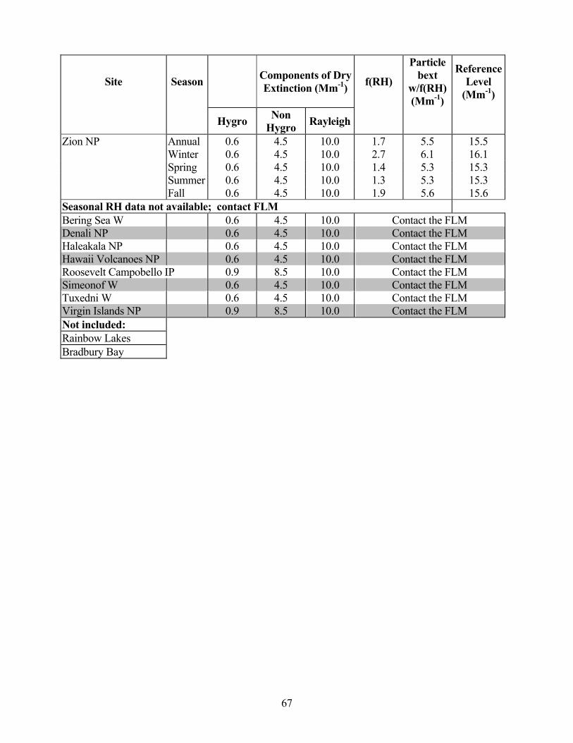
67


Particle bext

w/f(RH) (Mm-1)

Reference Level

(Mm-1)


Zion NP Annual 0.6 4.5 10.0 1.7 5.5 15.5 Winter 0.6 4.5 10.0 2.7 6.1 16.1 Spring 0.6 4.5 10.0 1.4 5.3 15.3 Summer 0.6 4.5 10.0 1.3 5.3 15.3 Fall 0.6 4.5 10.0 1.9 5.6 15.6

Seasonal RH data not available; contact FLM Bering Sea W 0.6 4.5 10.0 Contact the FLM Denali NP 0.6 4.5 10.0 Contact the FLM Haleakala NP 0.6 4.5 10.0 Contact the FLM Hawaii Volcanoes NP 0.6 4.5 10.0 Contact the FLM Roosevelt Campobello IP 0.9 8.5 10.0 Contact the FLM Simeonof W 0.6 4.5 10.0 Contact the FLM Tuxedni W 0.6 4.5 10.0 Contact the FLM Virgin Islands NP 0.9 8.5 10.0 Contact the FLM Not included: Rainbow Lakes Bradbury Bay

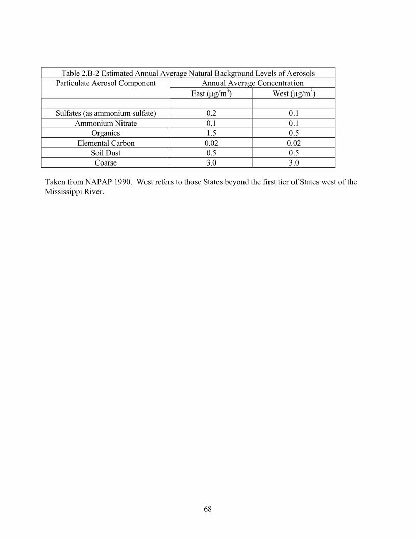
68

Table 2.B-2 Estimated Annual Average Natural Background Levels of Aerosols

Annual Average Concentration Particulate Aerosol Component East (µg/m3) West (µg/m3)

Sulfates (as ammonium sulfate) 0.2 0.1

Ammonium Nitrate 0.1 0.1 Organics 1.5 0.5

Elemental Carbon 0.02 0.02 Soil Dust 0.5 0.5 Coarse 3.0 3.0

Taken from NAPAP 1990. West refers to those States beyond the first tier of States west of the Mississippi River.

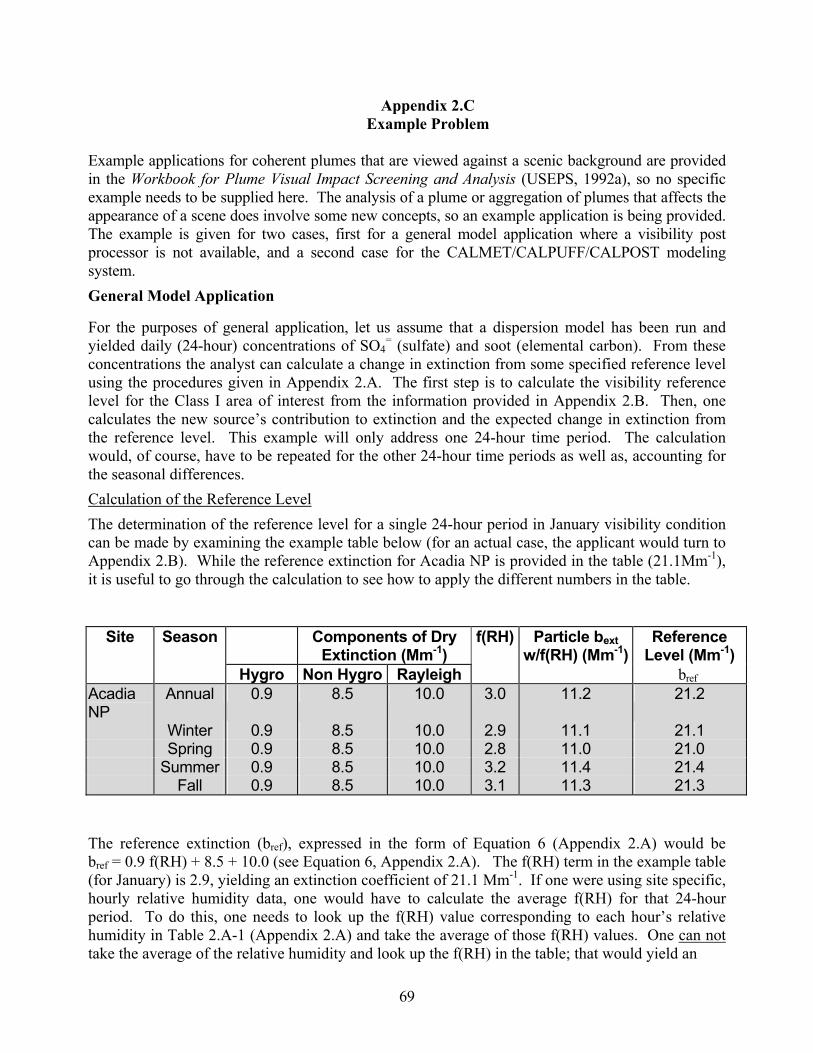
69

Appendix 2.C

Example Problem Example applications for coherent plumes that are viewed against a scenic background are provided in the Workbook for Plume Visual Impact Screening and Analysis (USEPS, 1992a), so no specific example needs to be supplied here. The analysis of a plume or aggregation of plumes that affects the appearance of a scene does involve some new concepts, so an example application is being provided. The example is given for two cases, first for a general model application where a visibility post processor is not available, and a second case for the CALMET/CALPUFF/CALPOST modeling system. General Model Application

For the purposes of general application, let us assume that a dispersion model has been run and yielded daily (24-hour) concentrations of SO4

= (sulfate) and soot (elemental carbon). From these concentrations the analyst can calculate a change in extinction from some specified reference level using the procedures given in Appendix 2.A. The first step is to calculate the visibility reference level for the Class I area of interest from the information provided in Appendix 2.B. Then, one calculates the new source’s contribution to extinction and the expected change in extinction from the reference level. This example will only address one 24-hour time period. The calculation would, of course, have to be repeated for the other 24-hour time periods as well as, accounting for the seasonal differences. Calculation of the Reference Level The determination of the reference level for a single 24-hour period in January visibility condition can be made by examining the example table below (for an actual case, the applicant would turn to Appendix 2.B). While the reference extinction for Acadia NP is provided in the table (21.1Mm-1), it is useful to go through the calculation to see how to apply the different numbers in the table.

Site Season Components of Dry

Extinction (Mm-1) Particle bext

w/f(RH) (Mm-1) Reference

Level (Mm-1) Hygro Non Hygro Rayleigh

f(RH)

bref Acadia NP

Annual 0.9 8.5 10.0 3.0 11.2 21.2

Winter 0.9 8.5 10.0 2.9 11.1 21.1 Spring 0.9 8.5 10.0 2.8 11.0 21.0 Summer 0.9 8.5 10.0 3.2 11.4 21.4 Fall 0.9 8.5 10.0 3.1 11.3 21.3

The reference extinction (bref), expressed in the form of Equation 6 (Appendix 2.A) would be bref = 0.9 f(RH) + 8.5 + 10.0 (see Equation 6, Appendix 2.A). The f(RH) term in the example table (for January) is 2.9, yielding an extinction coefficient of 21.1 Mm-1. If one were using site specific, hourly relative humidity data, one would have to calculate the average f(RH) for that 24-hour period. To do this, one needs to look up the f(RH) value corresponding to each hour’s relative humidity in Table 2.A-1 (Appendix 2.A) and take the average of those f(RH) values. One can not take the average of the relative humidity and look up the f(RH) in the table; that would yield an

70

incorrect result. (Similarly, the f(RH) values shown in the example table and in Appendix 2.B are generated using annual and seasonal average relative humidity estimates and the empirical curve for f(RH) given in IMPROVE 2000. Annual and seasonal averages of f(RH) do not directly correspond to the relative humidity values in Table 2.A-1.) Calculation of Single-Source Contribution In a typical modeling analysis, IWAQM recommends, and the FLMs endorse, the use of five years of meteorological data. This will produce a corresponding number of block 24-hour averaging periods, which will each need to be compared with the reference condition.

Again for purposes of illustration we will only show the calculation of extinction for one modeled 24-hour period in January. This calculation would then have to be repeated for all other 24-hour periods. For this example we will assume that the sources in the analysis contributed 0.3 µg/m3 of sulfate (SO4

=) and 0.10 µg/m3 of soot (elemental carbon), 24-hour average. The first step is to convert the mass of SO4

= to ammonium sulfate ((NH4)2SO4), which is accomplished by multiplying by the ratio of the molecular weights of (NH4)2SO4 to SO4

=, which is 1.375. This yields a concentration of (NH4)2SO4 of 0.4 µg/m3. This is then multiplied by the “dry” scattering efficiency of (NH4)2SO4 (which is 3, from Appendix 2.A, Equation 3), yielding an extinction coefficient for the sulfate of 1.2 Mm-1; the relative humidity adjustment has not yet been applied.

In this example our modeling does not require any conversion of the mass of soot, so we will just multiply the soot concentration (0.10 µg/m3) by the extinction efficiency of elemental carbon (which is 10, from Appendix 2.A, Equation 4). This yields an extinction coefficient of 1.0 Mm-1. Therefore, following the form of Equations 3 and 5 (Appendix 2.A), the source contribution would be:

bsource = 1.2 f(RH) + 1.0

A representative relative humidity adjustment term, f(RH), must be applied. It is important that the same adjustment be made to both the source contribution to extinction and the reference level. For a screening level analysis, the relative humidity adjustment factors listed in Appendix 2.B can be applied to the source contributions. For example, if we are analyzing for Acadia NP, the average winter f(RH) is 2.9. With the winter quarterly average relative humidity adjustment factor (f(RH)) of 2.9, bsource would be 4.5 Mm-1. Calculation of the Change in Extinction The resulting percent change in extinction is found from:

∆bext = (bsource/bref) × 100%

For the example here, bsource = 4.5 Mm-1 and bref = 22.1 Mm-1, yielding ∆bext = 20%. This calculation must be repeated for each 24-hour averaging period. To portray the frequency, magnitude, and geographic extent of expected impairment, this calculation will have to be repeated for all days and many receptors in the modeling domain. FLAG expects a robust selection of model receptor locations in the Class I area be included in the analyses, i.e., one receptor representing the entire area, or just the nearest boundary, will not be sufficient.

71

Example using the CALMET/CALPUFF/CALPOST modeling system

For the refined analysis, it is necessary to calculate the change in extinction for the relative humidity conditions on a specific day. To accomplish this, the representative, hourly RH values for this day need to be obtained. For each hour, the corresponding f(RH) must be obtained from Table 2.A-1. These f(RH) values are then averaged together. These calculations would have to be repeated for each 24-hour average concentration, at each receptor, in the analysis, using the corresponding average f(RH), and be applied to both the aerosol data in Table 2.B-1 (to determine the reference level) and the source contribution to extinction.

In the case of a CALPUFF application, the post-processor, CALPOST, has been set up to directly calculate the combined visibility effects from different visibility impairing pollutants. Refer to Figure 2.C-1 for an example of the visibility parameters to set in the CALPOST input file. Most of the parameters set in CALPOST are application specific. The pollutants in the example are sulfate and soot (elemental carbon). CALPOST allows for the specification of sulfate (SO4), but not elemental carbon in the source portion of the visibility calculation. (This should be rectified in the next update of the modeling system.) Therefore elemental carbon will be modeled as PM fine (PMF). In CALPOST the variables LVSO4 and LVPMF are set to true. Since elemental carbon is being modeled as PMF, the extinction efficiency for PMF must be set to that for elemental carbon (EEPMF = 10.0). FLAG is recommending that the default f(RH) values in Appendix 2.B be used for screening analyses for each Class I area. Therefore, MVISBK would be set to 6. When MVISBK is set to 6, RHFAC would be set to the f(RH) value in Appendix 2.B or in this example, it would be set to 2.9 for the winter months (Dec, Jan, Feb). CALPOST does not explicitly allow for the input of the hygroscopic and non-hygroscopic components to extinction at this time; it only allows for the input of the concentrations of particulate species. To properly input the components to extinction, the hygroscopic component of extinction is divided by 3 (the extinction efficiency of sulfate and nitrate) and is input to the variable BKSO4. In this example the hygroscopic component of extinction is 0.9; after dividing by 3 we get a value of 0.3, which is input to CALPOST (BKSO4 = 0.3). For the non-hygroscopic component, enter its value into the variable BKSOIL (BKSOIL = 8.5) (also make sure that EESOIL is set to 1.0). All other background concentrations must be set to zero (0.0). Finally, a value for the extinction due to Rayleigh scattering must be entered (BEXTRAY = 10.0). If MVISBK=2 (hour-by-hour calculation of f(RH)) in the above example, the hour-by-hour relative humidity values from CALMET would be used to calculate the 24-hour average extinction, rather than the long-term average f(RH) values supplied in Appendix 2.B. The only modification to the input would be that the value of RHMAX (set to 98.0 in the example) would be used to cap the maximum f(RH) used in the averages, and the value of RHFAC would not be used. A “vis.dat” file (not shown in Figure 2.C-1) would also be specified. It must be generated when CALPUFF is run.

72

Figure 2.C-1. Segment of CALPOST input file corresponding to example problem. --------------------------------------------------------------------------- INPUT GROUP: 2 -- Visibility Parameters (ASPEC = VISIB) -------------- Maximum relative humidity (%) used in particle growth curve (RHMAX) -- Default: 98 ! RHMAX = 98.0 ! Modeled species to be included in computing the light extinction Include SULFATE? (LVSO4) -- Default: T ! LVSO4 = T ! Include NITRATE? (LVNO3) -- Default: T ! LVNO3 = F ! Include ORGANIC CARBON? (LVOC) -- Default: T ! LVOC = F ! Include COARSE PARTICLES? (LVPMC) -- Default: T ! LVPMC = F ! Include FINE PARTICLES? (LVPMF) -- Default: T ! LVPMF = T ! And, when ranking for TOP-N, TOP-50, and Exceedance tables, Include BACKGROUND? (LVBK) -- Default: T ! LVBK = T ! Species name used for particulates in MODEL.DAT file COARSE (SPECPMC) -- Default: PMC ! SPECPMC = PMC ! FINE (SPECPMF) -- Default: PMF ! SPECPMF = PMF ! Extinction Efficiency (1/Mm per ug/m**3) ---------------------------------------- MODELED particulate species: PM COARSE (EEPMC) -- Default: 0.6 ! EEPMC = 0.6 ! PM FINE (EEPMF) -- Default: 1.0 ! EEPMF = 10.0 ! BACKGROUND particulate species: PM COARSE (EEPMCBK) -- Default: 0.6 ! EEPMCBK = 0.6 ! Other species: AMMONIUM SULFATE (EESO4) -- Default: 3.0 ! EESO4 = 3.0 ! AMMONIUM NITRATE (EENO3) -- Default: 3.0 ! EENO3 = 3.0 ! ORGANIC CARBON (EEOC) -- Default: 4.0 ! EEOC = 4.0 ! SOIL (EESOIL)-- Default: 1.0 ! EESOIL = 1.0 ! ELEMENTAL CARBON (EEEC) -- Default: 10. ! EEEC = 10.0 !

Set RHMAX = 98.0 (for MVISBK=2)

Set the flags for the pollutants modeled. In the example problem SO4 and EC (Modeled as PMF)

Note: in the example problem, the source’s elemental carbon (EC) is modeled as PMFINE (PMF). To calculate the extinction for EC as PMF the variable EEPMF needs to be reset to 10.0

73

Figure 2.C-1 (Cont). Segment of CALPOST input file corresponding to example problem.

Background Extinction Computation --------------------------------- Method used for background light extinction (MVISBK) -- Default: 6 ! MVISBK = 2 ! 1 = Supply single light extinction and hygroscopic fraction IWAQM (1993) RH adjustment applied to hygroscopic background and modeled sulfate and nitrate 2 = Compute extinction from speciated PM measurements (A) - Hourly RH adjustment applied to observed and modeled sulfateand nitrate - RH factor is capped at RHMAX 3 = Compute extinction from speciated PM measurements (B) - Hourly RH adjustment applied to observed and modeled sulfate and nitrate - Receptor-hour excluded if RH>RHMAX - Receptor-day excluded if fewer than 6 valid receptor-hours 4 = Read hourly transmissometer background extinction measurements - Hourly RH adjustment applied to modeled sulfate and nitrate - Hour excluded if measurement invalid (missing, interference, or large RH) - Receptor-hour excluded if RH>RHMAX - Receptor-day excluded if fewer than 6 valid receptor-hours 5 = Read hourly nephelometer background extinction measurements - Rayleigh extinction value (BEXTRAY) added to measurement - Hourly RH adjustment applied to modeled sulfate and nitrate - Hour excluded if measurement invalid (missing, interference, or large RH) - Receptor-hour excluded if RH>RHMAX - Receptor-day excluded if fewer than 6 valid receptor-hours 6 = Compute extinction from speciated PM measurements - FLAG RH adjustment factor applied to observed and modeled sulfate and nitrate

For Screening Analysis MVISBK = 6 Set RHFAC below

For Refined Analysis use MVISBK = 2

Specify a “vis.dat” file in CALPUFF

74

Figure 2.C-1 (Cont). Segment of CALPOST input file corresponding to example problem.

Additional inputs used for MVISBK = 6: -------------------------------------- Extinction coefficients for hygroscopic species (modeled and background) are computed using a monthly RH adjustment factor in place of an hourly RH factor (VISB.DAT file is NOT needed). Enter the 12 monthly factors here (RHFAC). Month 1 is January. (RHFAC) -- No default ! RHFAC = 2.9, 2.9, 2.8, 2.8, 2.8, 3.2, 3.2, 3.2, 3.1, 3.1, 3.1, 2.9 ! Additional inputs used for MVISBK = 2,3,6: ---------------------------------------- Background extinction coefficients are computed from monthly CONCENTRATIONS of ammonium sulfate (BKSO4), ammonium nitrate (BKNO3), coarse particulates (BKPMC), organic carbon (BKOC), soil (BKSOIL), and elemental carbon (BKEC). Month 1 is January. (ug/m**3) (BKSO4) -- No default ! BKSO4 = 0.3, 0.3, 0.3, 0.3, 0.3, 0.3, 0.3, 0.3, 0.3, 0.3, 0.3, 0.3 ! (BKNO3) -- No default ! BKNO3 = 0.0, 0.0, 0.0, 0.0, 0.0, 0.0, 0.0, 0.0, 0.0, 0.0, 0.0, 0.0 ! (BKPMC) -- No default ! BKPMC = 0.0, 0.0, 0.0, 0.0, 0.0, 0.0, 0.0, 0.0, 0.0, 0.0, 0.0, 0.0 ! (BKOC) -- No default ! BKOC = 0.0, 0.0, 0.0, 0.0, 0.0, 0.0, 0.0, 0.0, 0.0, 0.0, 0.0, 0.0 ! (BKSOIL) -- No default ! BKSOIL= 8.5, 8.5, 8.5, 8.5, 8.5, 8.5, 8.5, 8.5, 8.5, 8.5, 8.5, 8.5 ! (BKEC) -- No default ! BKEC = 0.0, 0.0, 0.0, 0.0, 0.0, 0.0, 0.0, 0.0, 0.0, 0.0, 0.0, 0.0 ! Additional inputs used for MVISBK = 2,3,5,6: ------------------------------------------ Extinction due to Rayleigh scattering is added (1/Mm) (BEXTRAY) -- Default: 10.0 ! BEXTRAY = 10.0 !

For screening analysis set monthly f(RH) values from Appendix 2.B

Background extinction values (Appendix 2.B) set to: BKSO4 = Hygroscopic / 3 BKSOIL = Non-Hygroscopic BKNO3, BKPMC, BKOC, BKEC = 0.0

75

3. OZONE a. Introduction Ozone is a toxic air pollutant that is formed on warm, sunny days when its precursors nitrogen oxides (NOx) and volatile organic compounds (VOC) react in the presence of sunlight. Because ozone is a regional pollutant, precursor sources both near and far from FLM areas can contribute to ozone formation. High ozone exposure can harm human health (U.S. EPA, 1996). Ozone is also phytotoxic, causing considerable damage to vegetation throughout the world. Some plant species are more sensitive to ozone than are humans (U.S. EPA, 1996). The primary National Ambient Air Quality Standard (NAAQS) for ozone is designed to protect human health, and the secondary NAAQS is set to achieve protection of the public welfare, including vegetation. The primary and secondary standards for ozone are the same. The new 8-hour, 0.08 ppm NAAQS for ozone is expected to be more protective of vegetation than the 1-hour, 0.12 ppm NAAQS.1 Attaining and maintaining compliance with the NAAQS is the responsibility of states and EPA rather than the FLMs. FLAG guidelines are not for regulatory purposes, but provide guidance for the FLM to identify ozone impacts on lands they manage. FLAG recognizes that specific relationships between precursor emissions and ambient ozone concentrations at a FLM area are difficult to quantify. Further, it is difficult to quantify the specific relationship between ambient ozone at a FLM area and vegetation response. Therefore, FLAG has chosen to focus on the effects of ozone on vegetation and the levels of ozone generally known to be phytotoxic in FLM areas as indicators of concern regarding ozone impacts on AQRVs. The objectives of this chapter are to document information currently known about vegetation response to ozone exposure, and to describe FLM procedures for responding to new source review (NSR) permit applications. If the FLMs have evidence that ozone is adversely impacting an area they manage, they will work to restrict further emissions of ozone precursors until those adverse impacts are mitigated. b. Ozone Effects on Vegetation Most ozone effects research has focused on agricultural crops because of the large economic losses that have been documented. Nevertheless, research has identified many native plants in natural ecosystems that are sensitive to ozone (U.S. EPA, 1996). Some of these ozone-sensitive plant species have been used as “bioindicators” of ozone to document phytotoxicity of ozone in the field due to ambient ozone. A listing of key literature describing known ozone effects on native vegetation is provided in Appendix H. The definitions for ozone injury and damage used by FLMs are based on the classical definitions (for example, see Guderian 1977). Injury is all physical or biological responses to pollutants, such as change in metabolism, reduced photosynthesis, leaf necrosis, premature leaf drop, and chlorosis. Damage is reduction in the intended use or value of the biological or physical resource; for example,

1The new 8-hour standard is currently being challenged in court and is not yet enforced; the 1-hour standard is still in effect.

76

economic production, ecological structure and function, aesthetic value, and biological or genetic diversity that may be altered through the impact of pollutants. Ozone enters plants through leaf stomata. It oxidizes plant tissue, causing changes in biochemical and physiological processes. These biochemical and physiological changes occur within the leaf long before visible necrotic symptoms appear (Guderian et al.1985). Plants must expend energy to detoxify ozone and repair injured tissue that could otherwise be used for growth or for maintenance of plant health. The injured plant cells eventually die if detoxification and repair cannot keep up with ozone uptake. The mesophyll cells under the upper epidermis of leaves are the most sensitive to ozone, and those are the first cells to die. The adjacent epidermal cells then die, forming a small black or brown interveinal necrotic lesion that becomes visible on the upper surface of the leaf. These visible lesions most frequently begin to develop on leaves that have just become fully matured, with older leaves on a stem showing increased amounts of injury. These lesions, termed oxidant stipple2, are quite specific indicators that the plant has been exposed to ozone. Other plant symptoms that can result from exposure to ozone, with or without the presence of oxidant stipple, include chlorosis, premature senescence, and reduced growth. However, these symptoms are non-specific for ozone since other stressors can also cause them to occur. Further, these non-specific symptoms are difficult to quantify in natural ecosystems, although limited data are available from exposure response experiments to estimate growth losses from specific ozone exposures. In general, the only indicator that a FLM has to document that ozone has impacted vegetation is visible symptoms of injury such as oxidant stipple. In addition to affecting individual plants, ozone can also affect entire ecosystems. Research shows that plants growing in areas with high exposure to ambient ozone may undergo natural selection for ozone tolerance (U.S. EPA, 1996). The final result could be the elimination of the most ozone-sensitive genotypes from the area. Regardless of the amount of ozone exposure, the magnitude of plant response may vary depending on the geographic area because of changes in meteorological and climatic conditions, and differences in plant conditions in space and time. Factors of most importance that influence plant response to ozone are the species/genotype, soil moisture, and nitrogen availability. Other factors influencing plant response to ozone include nutrient status, atmospheric humidity, temperature, solar radiation, phenological stage of development, day length, regional climatic differences, other pollutant interactions, and population/ecosystem interactions (U.S. EPA, 1996). Ozone-induced physiological changes and/or growth reductions in plants may exist long before necrotic lesions appear on foliage; however, it is very difficult to attribute these effects directly to ozone. Similarly, changes in growth, ecosystem form or function, or biological or genetic diversity caused by ozone are difficult to document in natural ecosystems. Limited data are available regarding injury and growth response to specific ozone exposures. Given the difficulty in determining ozone-induced physiological or growth changes in natural ecosystems, FLMs will utilize as indicators of ozone effects on vegetation (1) symptoms that are clearly ozone induced such as oxidant stipple, and (2) ozone exposures that have been shown to be phytotoxic.

2Specific symptoms of ozone injury in some plant species are different. A few species develop white or tan rather than brown or black lesions. This is termed “fleck” or “weather fleck” instead of oxidant stipple. In conifers, ozone causes banding of necrotic and green tissue near the tips of older needles, termed “chlorotic mottle.”

77

c. Recommended Metric to Determine Phytotoxic Ozone Concentrations Various metrics have been used to relate ozone exposure to plant response. Biologically relevant ozone metrics for plants cannot be directly related to, nor can they be calculated from, the 8-hour NAAQS for ozone. The NAAQS ozone metric does not directly account for peak concentrations, nor does it accumulate exposure, important parameters in any biologically relevant ozone metric. Biologically relevant metrics considered by FLAG include the W126, SUM06, AOT40, and ozone flux. The W126 is an index that uses a sigmoidal weighted function to weight each hourly ozone concentration. The W126 index is determined by summing all the sigmoidal weighted concentrations for a specified time period (Lefohn and Runeckles, 1987). The W126 index was described and used in EPA’s Air Quality Criteria for Ozone and Related Photochemical Oxidants, Vol. II (U.S. EPA, 1996) to characterize ozone trends. FLMs will use the W126 metric to determine phytotoxic ozone concentrations in FLM areas. The W126 is preferred to other cumulative metrics for a couple of reasons. First, the W126 preferentially weights the peak exposures, whereas other metrics, such as the AOT40 or the SUM06, do not. Second, the W126 accumulates ozone exposures at lower concentrations than does the AOT40 or SUM06. The AOT40 and SUM06 only accumulate concentrations above their particular threshold, e.g., 40 ppb for AOT40 and 60 ppb for SUM06. Phytotoxic effects have been shown to occur at exposure concentrations below 60 ppb (U.S. EPA 1996). The AOT40 metric is commonly used in Europe. Some European scientists recently have concluded that the AOT40 metric is useful for exceedance mapping but not for assessment of biomass loss (Kaerenlampi and Skaerby 1996). Therefore, FLAG does not recommend the AOT40 for FLM assessments. The SUM06, W126, and AOT40 are ambient ozone exposure parameters, whereas flux is an ozone dose parameter for internal uptake. Flux is determined from ambient ozone concentration at the leaf surface and stomatal conductance. Ozone uptake relates more closely to plant response than does ambient ozone exposure. However, detoxification of ozone once it enters the plant is also an important component of plant response, and measuring uptake alone will not necessarily reflect the potential plant response. A benefit of flux is that it might allow differential weighting of daytime versus nighttime exposure (with daytime being weighted more heavily in most cases). Science has not advanced sufficiently for FLAG to recommend use of flux as a metric for plant response to ozone at this time. However, research on the use of flux as an ozone metric is continuing (Massman et al. 2000) and it will be examined for possible future use. To use the W126 metric, the daily and seasonal time periods of measurement must also be determined. Although most ozone uptake occurs during the day, many plant species can have nighttime stomatal conductance resulting in ozone uptake (Musselman and Minnick 2000). Nighttime uptake is a function of many variables, including species, region (e.g., desert, deciduous forest, etc.), season, and elevation. In addition, many FLM areas, particularly those in mountainous regions, have high nighttime ozone exposures. Further, plants may be more sensitive to ozone at night (Musselman and Minnick 2000). Therefore, FLAG endorses use of a 24-hour time period for the W126 metric. Plant sensitivity and exposure to ozone will change throughout the growing season. Use of a rolling 90-day cumulative value for the W126 metric would account for changes in exposure over the season. However, some vegetation exposure/response and ozone monitoring data are currently available using 7-month (April through October) seasonal cumulative W126 values. In order to take advantage of this existing information, FLAG will use the April-October time period for the W126 metric.

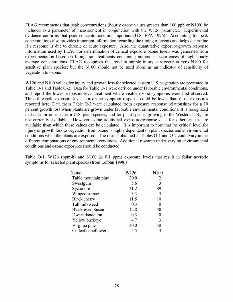
78

FLAG recommends that peak concentrations (hourly ozone values greater than 100 ppb or N100) be included as a parameter of measurement in conjunction with the W126 parameter. Experimental evidence confirms that peak concentrations are important (U.S. EPA 1996). Accounting for peak concentrations also provides important information regarding the timing of events and helps determine if a response is due to chronic or acute exposure. Also, the quantitative exposure/growth response information used by FLAG for determination of critical exposure ozone levels was generated from experimentation based on fumigation treatments containing numerous occurrences of high hourly average concentrations. FLAG recognizes that oxidant stipple injury can occur at zero N100 for sensitive plant species; but the N100 should not be used alone as an indicator of sensitivity of vegetation to ozone. W126 and N100 values for injury and growth loss for selected eastern U.S. vegetation are presented in Table O-1 and Table O-2. Data for Table O-1 were derived under favorable environmental conditions, and report the lowest exposure level treatment where visible ozone symptoms were first observed. Thus, threshold exposure levels for ozone symptom response could be lower than those exposures reported here. Data from Table O-2 were calculated from exposure response relationships for a 10 percent growth loss when plants are grown under favorable environmental conditions. It is recognized that data for other eastern U.S. plant species, and for plant species growing in the Western U.S., are not currently available. However, some additional exposure/response data for other species are available from which these values can be calculated. It is important to note that the critical level for injury or growth loss to vegetation from ozone is highly dependent on plant species and environmental conditions when the plants are exposed. The results obtained in Tables O-1 and O-2 could vary under different combinations of environmental conditions. Additional research under varying environmental conditions and ozone exposures should be conducted. Table O-1. W126 (ppm-h) and N100 (≥ 0.1 ppm) exposure levels that result in foliar necrotic symptoms for selected plant species (from Lefohn 1998.)

Name W126 N100 Table mountain pine 20.0 2 Sweetgum 5.6 3 Sycamore 31.2 89 Winged sumac 3.3 5 Black cherry 11.5 10 Tall milkweed 0.3 0 Black-eyed Susan 12.8 50 Dwarf dandelion 0.3 0 Yellow buckeye 4.7 3 Virginia pine 30.0 50 Cutleaf coneflower 5.5 3

79

Table O-2. W126 (ppm-h) and N100 (≥ 0.1 ppm) exposure levels that resulted in a 10 percent growth loss for selected plant species (from Lefohn 1998.)

Name W126 N100 Aspen 259 6.4 4 Aspen wild 71.4 243 Black Cherry 6.5 1 Red Maple 85.4 245 Whorled-wood aster 8.2 10 Yellow poplar 14.4 4 Eastern white pine 30.2 66 Sugar maple 44.7 131 Sycamore 15.4 27 Winged sumac 9.7 4

Ambient W126 and N100 values are available for many Class I areas in the eastern U.S., with values soon to be available for additional FLM areas. A table showing representative high and low W126 and N100 values for selected FLM areas is appended to this report (Appendix 3.B). Unfortunately, ambient ozone data are lacking for many western U.S. FLM areas, and large differences in terrain and elevation may limit the use of nearby data. d. Identification of Ozone Sensitive AQRVs or Sensitive Receptors FLMs have determined that given the high ecological, aesthetic, and intrinsic value of federal lands, all native species are significant and warrant protection. Ideally, protection efforts would focus on the identification and protection of the most sensitive species in an area. Unfortunately, AQRV identification is limited by incomplete species inventories and/or lack of exposure/response data for most species of native vegetation. Sensitive species identification will improve as more information becomes available. In the meantime, FLAG is providing a preliminary list of sensitive plant species for each Class I area, i.e., those species that have been observed to exhibit ozone symptoms at ambient ozone exposures (Appendix 3.A). Those ambient levels have not necessarily occurred at the specific Class I area where the plants occur. AQRV lists will be available in the Air Synthesis and NRIS-AIR databases (See Section B.4.f. of this report) and will be updated as necessary. e. Review Process for Sources that Could Affect Ozone Levels or Vegetation in FLM Areas As mentioned above, NOx and VOC are ozone precursors. States and the EPA have based ozone control strategies in various parts of the country on the determination of which precursor is most likely to influence the formation of ozone. Information suggests that in areas where ozone formation is driven by VOC emissions, i.e., VOC-limited areas, VOC to NOx ratios are less than 4:1. In VOC-limited areas, minimizing or reducing VOC emissions is the most effective means of limiting or lowering ozone concentrations. Conversely, in NOx-limited areas, where VOC to NOx ratios are greater than 15:1, controlling NOx emissions is most effective. It is generally thought that most rural areas of the U.S. are NOx-limited, most or all of the time, with the possible exception of the rural areas of southern California. The FLMs do not have current data to show that all areas are NOx limited, nor do they consider VOCs to be unimportant as ozone precursors. However, until there is enough information available for FLAG to determine whether ozone formation in each FLM area is primarily limited by NOx or VOC emissions, we will assume all FLM areas are NOx-limited and will focus on

80

control of NOx emissions. Where FLMs have information indicating a specific area is VOC limited, they will shift ozone protection strategy to focus on VOC rather than NOx emissions. Source/receptor modeling is required in most NSR permit applications for particulate matter, sulfur dioxide, and nitrogen dioxide. FLAG is aware of attempts by EPA and others to develop dispersion models that can relate emissions from a single source to changes in ozone concentrations. We recognize that there is currently no model available that can provide this kind of single source attribution information for ozone. Nevertheless, because of existing and suspected ozone concerns in a number of FLM areas (e.g., evidence of phytotoxic effects and high ambient concentrations), we will consider ozone effects when reviewing NSR permit applications. However, because single source attribution modeling is possible for both visibility and deposition, FLMs will be more concerned about ozone if modeling indicates NOx emissions are likely to cause an adverse impact on visibility, soils, and/or surface waters. The FLMs recognize that oxidant stipple can occur at hourly ozone concentrations that can be considered natural background levels (Singh et al. 1978). Many of the high hourly background concentrations can be attributed to stratospheric intrusions or stratospheric mixing in the upper troposphere (Singh et al. 1978); but stratospheric intrusions rarely occur in the middle and southern latitudes after May (Singh et al. 1980, Wooldridge et al. 1997), and thus do not coincide with the major portion of the growing season. However, oxidant stipple has been observed on foliage in the spring when these intrusions can occur. In general, oxidant stipple observed on foliage from June through September cannot be attributed to natural background ozone from stratospheric sources. Low levels of ambient ozone may occasionally occur in the troposphere from non-anthropogenic and non-stratospheric sources. The occurrence of oxidant stipple necrosis on plant foliage may indicate further ozone induced physiological and growth impacts. Point sources emit precursors that could produce ozone at the FLM area, and increased ozone could induce further injury or damage to vegetation. However, we assume that restriction on increases in ozone precursors will prevent additional ambient ozone and subsequent increases in injury or damage to vegetation in FLM managed areas. It is important that ambient ozone monitoring be conducted by the State or Local air pollution control agency or by the FLM to determine the seasonal ozone exposure. FLM actions or specific requests on a permit application will be based on the existing air pollution situation at the FLM area(s) that may be affected by the source. Some FLMs may rely on growth loss rather than foliar necrosis to make an adverse impact. Each FLM will determine if actions are warranted to limit emissions that might lead to increased ambient ozone, based on the expected impact of ozone in their particular area. FLM response will depend on whether or not:

1. ozone vegetation effects have been documented in the area (as evidenced by foliar injury or damage to vegetation);

2. ozone exposure levels occurring in the area are high enough that they could affect vegetation (i.e., ozone exposures are at levels shown to be phytotoxic).

Figure O-1 outlines the general FLM process for responding to NSR permit applications based on ozone exposure and vegetation effects at the receptor site. Management decisions regarding acceptance of an existing or future ozone exposure will be area-specific and may differ

81

significantly between agencies, or even regionally within agencies. Each FLM will determine if injury and/or damage are necessary to warrant action, based on the expected impact in the area they manage. The decisions are based on the FLM interpretation of regulations, past experience in the NSR arena, availability of ozone effect exposure/response information for species that occur in the area, and other factors. The FLM will negotiate with the NSR permit applicant and the permitting authority regarding the options listed in Figure O-1.

Figure O-1. FLM response to potential ozone effects from new emissions source.

No U Unknown Unknown Yes Yes No Unknown Yes No Items referenced in Figure O-1: a. The FLM may recommend one or more of the following:

- That the proposed source use stricter than BACT controls (e.g., Lowest Achievable Emission Rate [LAER]). - That the proposed source obtain NOx emission offsets that will benefit the potentially affected FLM area (as demonstrated by dispersion modeling). - That the permitting authority (i.e., state or EPA) conduct regional modeling to identify sources that are contributing significantly to ozone-associated impacts in the FLM area, and that the permitting authority then undertake actions necessary to reduce emissions from those sources (e.g., SIP revision).

a

FLM not likely to object to permit; FLM may ask for d

FLM not likely to object to permit

Ozone damage to vegetation

FLM not likely to object to permit; FLM may ask for c and/or d

a; FLM may ask for c

FLM not likely to object to permit; FLM may ask for c

START

Ozone damage to vegetation a

Ozoneexposurecurrently

recognized asphytotoxic; FLM

may ask for b

82

b. The applicant calculate the ozone exposure for vegetation (using W126 and N100 metrics) for the affected FLM area(s) where such information is not already available.

c. The permitting authority or applicant fund post-construction ambient ozone monitoring in or near the FLM area.

d. The applicant conduct or fund post-construction ozone effects surveys in the FLM area and/or exposure/response effects research.

Note: “Ozone exposure currently recognized as phytotoxic” is determined based on data from exposure response studies and ambient ozone at the site. The FLM may ask the applicant to calculate the ozone exposure values if these data are not already available. “Ozone damage to vegetation” is determined from field observations at the impacted site. f. Further Guidance to FLMs As mentioned above, limited information about ozone exposure/response relationships in plants and lack of an ozone source/receptor model make it difficult to protect FLM areas from the effects of ozone from new sources. However, there are other area-specific gaps in information that also limit protection efforts. It is important for local land managers to attempt to collect the missing information. This section provides guidance specifically to FLMs on what types of data should be collected and how the data could be collected.

Identifying and Monitoring Ozone-sensitive AQRVs Many FLM areas need more details regarding plant species presence, location, and abundance. FLAG recommends FLMs gather this information, where needed, and refine their lists of area-specific ozone-sensitive plants. FLMs are currently developing lists of sensitive species to crosscheck with the plant species list for their area to determine potential sensitivity to ozone. In the future, the FLMs will place ozone sensitive plant species lists in the NRIS-AIR or Air Synthesis databases for comparison to plant species lists for each wilderness area or national park. FLAG recommends that once local FLMs have developed lists of potentially sensitive AQRVs specific for their site, they conduct surveys to detect the presence of ozone-induced foliar injury on the selected species. The USDA/FS Forest Health Monitoring (FHM) Program has developed foliar injury survey protocols and QA/QC procedures that can be used to collect this information. Another resource is the foliar injury training module developed by the NPS Air Resources Division and Pennsylvania State University. This module helps field staff identify and quantify ozone injury symptoms on plant foliage. Field crews must obtain proper training and field experience in identifying foliar injury symptoms before surveys can be conducted. Ideally, to verify ozone-induced foliar injury symptoms in the field, exposure/response fumigation studies should be conducted on these species, using concentrations that reflect current ambient exposure. Plants should also be tested at higher exposures, simulating increased levels of ambient ozone that might occur in the future. Due to the expense of constructing and operating such systems, it would be most appropriate for agencies to join resources and develop regional fumigation facilities. At a minimum, such facilities should be constructed both in the eastern and western U.S., since ambient conditions at an eastern facility might not be appropriate for western species and vice versa.

83

Ambient Ozone Monitoring Many FLM areas do not currently have either on-site or nearby ambient ozone monitoring data. FLAG recommends that local FLMs make every effort to collect this information and that they use quality-assured ambient ozone monitoring protocols developed by the EPA and the state air quality agency. Continuous (active) monitoring is preferred since this type of data is necessary to determine compliance with the ozone NAAQS. Continuous monitoring is also necessary to determine the temporal dynamics of ozone exposure for vegetation, and is necessary to calculate the W126 and N100 parameters. Unfortunately, continuous monitoring is expensive and requires electric power that is often not available in or near remote FLM areas. When installing a continuous monitor is not an option, FLAG recommends use of passive monitors. Passive monitors give total exposure loading values (SUM00) for a specified period of time. The data are useful for indicating year-to-year changes in total ozone exposure at an individual site, and for indicating where continuous monitors should be installed. However, FLMs recognize the limitation of passive samplers in relating ozone exposure to plant response. g. Ozone Air Pollution Web Sites U.S. EPA ozone information: http://www.epa.gov/airlinks http://www.epa.gov gov/oar/oaqps/cleanair.html http://www.epa.gov/naaqsfin/o3health.htm http://www.epa.gov/acidrain/castnet NPS ozone information: http://www2.nature.nps.gov/ard/gas/network.htm; http://www2.nature.nps.gov/ard/veginj.htm Ozone effects research, USDA ARS, North Carolina: http://www.ces.ncsu.edu/depts/pp/notes/Ozone/ozone.html Ozone effects research, England: http://www.ncl.ac.uk/airweb/ozone/ozone.htm Ozone effects research, Switzerland: http://www.wsl.ch/forest/risks/wsidb/projects/ozone/ozoneENG.html Ozone exposure metrics for vegetation: http://www.asl-associates.com/ Ozone W126 calculator: http://216.48.37.155/calculator/index.htm

84

Appendix 3.A: A Preliminary Listing for Selected USDA/FS, NPS, and FWS Class I Areas of

Plant Species that have been Shown to be Sensitive Receptors for Ozone.

1. USDA/FS CLASS I WILDERNESS AREAS Alabama Sipsey

Black Cherry Prunus serotina Blackberry Rubus canadensis Sweetgum Liquidambar styraciflua Tulip Poplar Liriodendron tulipifera

Arkansas Upper Buffalo

Blackberry Rubus canadensis Arizona Chiricahua

Serviceberry Amelanchier alnifola Chokecherry Prunus virginiana

Globemallow Sphaeralcea Ponderosa Pine Pinus ponderosa

Skunkbush Rhus trilobata Galiuro

Serviceberry Amelanchier alnifola Chokecherry Prunus virginiana Globemallow Sphaeralcea

Ponderosa Pine Pinus ponderosa Skunkbush Rhus trilobata

Mazatzal Aspen Populus tremuloides

Ponderosa Pine Pinus ponderosa Skunkbush Rhus trilobata Mount Baldy

Arizona Willow Salix Ponderosa Pine Pinus ponderosa Western White Pine Pinus monticola Pine Mountain

Aspen Populus tremuloides Ponderosa Pine Pinus ponderosa

Skunkbush Rhus trilobata Sierra Ancha

Aspen Populus tremuloides Ponderosa Pine Pinus ponderosa Skunkbush Rhus trilobata Superstition

Aspen Populus tremuloides Ponderosa Pine Pinus ponderosa

Skunkbush Rhus trilobata Sycamore Canyon

Aspen Populus tremuloides Ponderosa Pine Pinus ponderosa Skunkbush Rhus trilobata

85

California Agua Tibia Jeffrey Pine Pinus jeffreyi Ponderosa Pine Pinus ponderosa Western White Pine Pinus monticola Ansel Adams Jeffrey Pine Pinus jeffreyi Limber Pine Pinus flexilis Lodgepole Pine Pinus contorta Ponderosa Pine Pinus ponderosa Western White Pine Pinus monticola Caribou Limber Pine Pinus flexilis Lodgepole Pine Pinus contorta Cucamonga

Jeffrey Pine Pinus jeffreyi Ponderosa Pine Pinus ponderosa Western White Pine Pinus monticola Desolation Limber Pine Pinus flexilis Lodgepole Pine Pinus contorta Dome Land Jeffrey Pine Pinus jeffreyi Limber Pine Pinus flexilis Lodgepole Pine Pinus contorta Ponderosa Pine Pinus ponderosa Western White Pine Pinus monticola Emmigrant Jeffrey Pine Pinus jeffreyi Limber Pine Pinus flexilis Ponderosa Pine Pinus ponderosa Hoover Ponderosa Pine Pinus ponderosa John Muir Jeffrey Pine Pinus jeffreyi Limber Pine Pinus flexilis Lodgepole Pine Pinus contorta Ponderosa Pine Pinus ponderosa Western White Pine Pinus monticola Kaiser Jeffrey Pine Pinus jeffreyi Limber Pine Pinus flexilis Lodgepole Pine Pinus contorta Ponderosa Pine Pinus ponderosa Western White Pine Pinus monticola Marble Mountain

Jeffrey Pine Pinus jeffreyi Limber Pine Pinus flexilis Lodgepole Pine Pinus contorta Ponderosa Pine Pinus ponderosa

Western White Pine Pinus monticola Mokelumme Jeffrey Pine Pinus jeffreyi Limber Pine Pinus flexilis Lodgepole Pine Pinus contorta Ponderosa Pine Pinus ponderosa Western White Pine Pinus monticola

86

San Gorgonio Jeffrey Pine Pinus jeffreyi Limber Pine Pinus flexilis Lodgepole Pine Pinus contorta Ponderosa Pine Pinus ponderosa

Western White Pine Pinus monticola San Jacinto Jeffrey Pine Pinus jeffreyi Limber Pine Pinus flexilis Lodgepole Pine Pinus contorta Ponderosa Pine Pinus ponderosa Western White Pine Pinus monticola San Rafael

Jeffrey Pine Pinus jeffreyi Ponderosa Pine Pinus ponderosa Western White Pine Pinus monticola South Warner Jeffrey Pine Pinus jeffreyi Limber Pine Pinus flexilis Lodgepole Pine Pinus contorta Ponderosa Pine Pinus ponderosa Western White Pine Pinus monticola Thousand Lakes Jeffrey Pine Pinus jeffreyi Limber Pine Pinus flexilis Lodgepole Pine Pinus contorta Ponderosa Pine Pinus ponderosa Western White Pine Pinus monticola Yolla Bolly - Middle Eel Jeffrey Pine Pinus jeffreyi Limber Pine Pinus flexilis Lodgepole Pine Pinus contorta Ponderosa Pine Pinus ponderosa Western White Pine Pinus monticola

Colorado Eagles Nest Subalpine fir Abies lasiocarpa White clover Trifolium repens Saskatoon serviceberry Amelanchier alnifolia Sagebrush Artemesia sp

Trembling aspen Populus tremuloides Chockcherry Prunus vierginiana Thimbleberry Rubus parviflorus Squawberry Rhus trilobata Huckleberry Vaccinium sp. Flat Tops Subalpine fir Abies lasiocarpa Boxelder Acer negundo Saskatoon serviceberry Amelanchier alnifolia Sagebrush Artemesia sp

Trembling aspen Populus tremuloides Chockcherry Prunus vierginiana Thimbleberry Rubus parviflorus Squawberry Rhus trilobata Huckleberry Vaccinium sp.

87

Maroon Bells – Snowmass White fir Abies concolor Subalpine fir Abies lasiocarpa Sagebrush Artemesia sp. Trembling aspen Populus tremuloides Mount Zirkel Subalpine fir Abies lasiocarpa Saskatoon serviceberry Amelanchier alnifolia Sagebrush Artemesia sp

Trembling aspen Populus tremuloides Chockcherry Prunus vierginiana Thimbleberry Rubus parviflorus Squawberry Rhus trilobata Huckleberry Vaccinium sp. Rawah White fir Abies concolor Subalpine fir Abies lasiocarpa Boxelder Acer negundo Saskatoon serviceberry Amelanchier alnifolia Sagebrush Artemesia sp

Trembling aspen Populus tremuloides Chockcherry Prunus vierginiana Thimbleberry Rubus parviflorus Squawberry Rhus trilobata Huckleberry Vaccinium sp. Weminuche White fir Abies concolor Subalpine fir Abies lasiocarpa Saskatoon serviceberry Amelanchier alnifolia Sagebrush Artemesia sp

Trembling aspen Populus tremuloides Chockcherry Prunus vierginiana Thimbleberry Rubus parviflorus Huckleberry Vaccinium sp. West Elk White fir Abies concolor Subalpine fir Abies lasiocarpa Boxelder Acer negundo Saskatoon serviceberry Amelanchier alnifolia Sagebrush Artemesia sp

Hybrid poplar Populus deloides x trichocarpa Ninebark Pysocarpus sp.

Chockcherry Prunus vierginiana Thimbleberry Rubus parviflorus Squawberry Rhus trilobata Huckleberry Vaccinium sp. Florida Bradwell Bay

Blackberry Rubus canadensis Staghorn Sumac Rhus typhina Sweetgum Liquidambar styraciflua Tulip Poplar Liriodendron tulipifera

88

Georgia Cohutta

Black Cherry Prunus serotina Blackberry Rubus canadensis Sweetgum Liquidambar styraciflua Tulip Poplar Liriodendron tulipifera

Idaho Sawtooth Ponderosa Pine Pinus ponderosa Minnesota Boundary Waters Canoe Area Aspen Populus tremuloides

Chokecherry Prunus virginiana Eastern White Pine Pinus strobus Missouri Hercules-Glades

Black Cherry Prunus serotina Elderberry Sambucus canadensis Milkweed Asclepias syriaca Tulip Poplar Liriodendron tulipifera White Ash Fraxinus americana

Nevada Jarbridge Ponderosa Pine Pinus ponderosa New Hampshire Great Gulf


Presidential Range - Dry River Black Cherry Prunus serotina Elderberry Sambucus canadensis Milkweed Asclepias syriaca Red Spruce Picea rubens White Ash Fraxinus americana

North Carolina Joyce Kilmer - Slickrock

American Sycamore Platinus occidentalis Black Cherry Prunus serotina Blackberry Rubus canadensis Elderberry Sambucus canadensis

Flowering Dogwood Cornus florida Pin Cherry Prunus pensylvanica Poison Ivy Rhus radicans Red Maple Acer rubrum Red Oak Quercus rubra Sassafrass Sassafras albidum Sweetgum Liquidambar styraciflua Tulip Poplar Liriodendron tulipifera White Ash Fraxinus americana

Eastern White Pine Pinus strobus

89

Linville Gorge

American Sycamore Platinus occidentalis Black Cherry Prunus serotina Blackberry Rubus canadensis

Flowering Dogwood Cornus florida Red Maple Acer rubrum Red Oak Quercus rubra Sassafrass Sassafras albidum Sweetgum Liquidambar styraciflua Tulip Poplar Liriodendron tulipifera

Eastern White Pine Pinus strobus Shining Rock

Black Cherry Prunus serotina Black-Eyed Susan Rudbeckia hirta Blackberry Rubus canadensis

Chokecherry Prunus virginiana Flowering Dogwood Cornus florida Milkweed Asclepias syriaca Poison Ivy Rhus radicans Red Oak Quercus rubra Sassafrass Sassafras albidum Tulip Poplar Liriodendron tulipifera White Ash Fraxinus americana

Eastern White Pine Pinus strobus Oregon* Diamond Peak Western Serviceberry Amelancier alnifolia Quaking Aspen Populus tremuloides Scouler Willow Salix scouleriana Thin-leaved Huckleberry Vaccinium membranaceum Red Alder Alnus rubra Mountain Ash Sorbus sitchensis Black Twin-berry Lonicera involucrata Stink Currant Ribes bracteosum Eagle Cap Western Serviceberry Amelancier alnifolia Ponderosa Pine Pinus ponderosa Quaking Aspen Populus tremuloides Scouler Willow Salix scouleriana Thin-leaved Huckleberry Vaccinium membranaceum Mountain Ash Sorbus sitchensis Black Twin-berry Lonicera involucrata Gearhart Mountain Western Serviceberry Amelancier alnifolia Quaking Aspen Populus tremuloides Scouler Willow Salix scouleriana Thin-leaved Huckleberry Vaccinium membranaceum Mountain Ash Sorbus sitchensis Black Twin-berry Lonicera involucrata

*Plant species listed for Oregon have been identified as ozone sensitive in laboratory fumigations. Ozone injury to some of these species has not been verified in the field.

90

Hells Canyon Western Serviceberry Amelancier alnifolia Ponderosa Pine Pinus ponderosa Quaking Aspen Populus tremuloides Scouler Willow Salix scouleriana Black Twin-berry Lonicera involucrata Mallow Ninebark Physocarpus malvaceus Black Cottonwood Populus trichocarpa Kalmiopsis Western Serviceberry Amelancier alnifolia Scouler Willow Salix scouleriana Thin-leaved Huckleberry Vaccinium membranaceum Mountain Ash Sorbus sitchensis Black Twin-berry Lonicera involucrata Mount Hood Western Serviceberry Amelancier alnifolia Pacific ninebark Physocarpus capitatus Quaking Aspen Populus tremuloides Scouler Willow Salix scouleriana Thin-leaved Huckleberry Vaccinium membranaceum Red Alder Alnus rubra Mountain Ash Sorbus sitchensis Black Twin-berry Lonicera involucrata Black Cottonwood Populus trichocarpa Stink Currant Ribes bracteosum Mount Jefferson Western Serviceberry Amelancier alnifolia Quaking Aspen Populus tremuloides Scouler Willow Salix scouleriana Thin-leaved Huckleberry Vaccinium membranaceum Red Alder Alnus rubra Mountain Ash Sorbus sitchensis Black Twin-berry Lonicera involucrata Black Cottonwood Populus trichocarpa Stink Currant Ribes bracteosum Mount Washington Western Serviceberry Amelancier alnifolia Scouler Willow Salix scouleriana Thin-leaved Huckleberry Vaccinium membranaceum Red Alder Alnus rubra Mountain Ash Sorbus sitchensis Black Twin-berry Lonicera involucrata Stink Currant Ribes bracteosum Mountain Lakes Western Serviceberry Amelancier alnifolia Pacific ninebark Physocarpus capitatus Ponderosa Pine Pinus ponderosa Quaking Aspen Populus tremuloides Scouler Willow Salix scouleriana Thin-leaved Huckleberry Vaccinium membranaceum Red Alder Alnus rubra Mountain Ash Sorbus sitchensis Black Twin-berry Lonicera involucrata Black Cottonwood Populus trichocarpa

91

Strawberry Mountain Western Serviceberry Amelancier alnifolia Ponderosa Pine Pinus ponderosa Quaking Aspen Populus tremuloides Scouler Willow Salix scouleriana Thin-leaved Huckleberry Vaccinium membranaceum Mountain Ash Sorbus sitchensis Black Twin-berry Lonicera involucrata Three Sisters Western Serviceberry Amelancier alnifolia Pacific ninebark Physocarpus capitatus Ponderosa Pine Pinus ponderosa Quaking Aspen Populus tremuloides Scouler Willow Salix scouleriana Thin-leaved Huckleberry Vaccinium membranaceum Mountain Ash Sorbus sitchensis Black Twin-berry Lonicera involucrata Vermont Lye Brook

Black Cherry Prunus serotina Elderberry Sambucus canadensis Milkweed Asclepias syriaca Red Spruce Picea rubens White Ash Fraxinus americana

Virginia James River Face

Black Cherry Prunus serotina Blackberry Rubus canadensis Chokecherry Prunus virginiana

Flowering Dogwood Cornus florida Milkweed Asclepias syriaca Poison Ivy Rhus radicans Red Oak Quercus rubra Sassafrass Sassafras albidum Sweetgum Liquidambar styraciflua Tulip Poplar Liriodendron tulipifera White Ash Fraxinus americana

Eastern White Pine Pinus strobus Washington* Alpine Lakes Western Serviceberry Amelancier alnifolia Scouler Willow Salix scouleriana Thin-leaved Huckleberry Vaccinium membranaceum Red Alder Alnus rubra Mountain Ash Sorbus sitchensis Black Twin-berry Lonicera involucrata Stink Currant Ribes bracteosum

*Plant species listed for Washington have been identified as ozone sensitive in laboratory fumigations. Ozone injury to some of these species has not been verified in the field.

92

Glacier Peak Western Serviceberry Amelancier alnifolia Pacific ninebark Physocarpus capitatus Scouler Willow Salix scouleriana Thin-leaved Huckleberry Vaccinium membranaceum Red Alder Alnus rubra Mountain Ash Sorbus sitchensis Black Twin-berry Lonicera involucrata Black Cottonwood Populus trichocarpa Stink Currant Ribes bracteosum Goat Rocks Western Serviceberry Amelancier alnifolia Pacific ninebark Physocarpus capitatus Scouler Willow Salix scouleriana Thin-leaved Huckleberry Vaccinium membranaceum Red Alder Alnus rubra Mountain Ash Sorbus sitchensis Black Twin-berry Lonicera involucrata Black Cottonwood Populus trichocarpa Stink Currant Ribes bracteosum Mount Adams Western Serviceberry Amelancier alnifolia Pacific ninebark Physocarpus capitatus Quaking Aspen Populus tremuloides Scouler Willow Salix scouleriana Thin-leaved Huckleberry Vaccinium membranaceum Red Alder Alnus rubra Mountain Ash Sorbus sitchensis Black Twin-berry Lonicera involucrata Black Cottonwood Populus trichocarpa Stink Currant Ribes bracteosum Paysayten Western Serviceberry Amelancier alnifolia Quaking Aspen Populus tremuloides Scouler Willow Salix scouleriana Thin-leaved Huckleberry Vaccinium membranaceum Mountain Ash Sorbus sitchensis Black Twin-berry Lonicera involucrata West Virginia Dolly Sods


Otter Creek Black Cherry Prunus serotina Elderberry Sambucus canadensis Milkweed Asclepias syriaca Red Spruce Picea rubens Tulip Poplar Liriodendron tulipifera White Ash Fraxinus americana

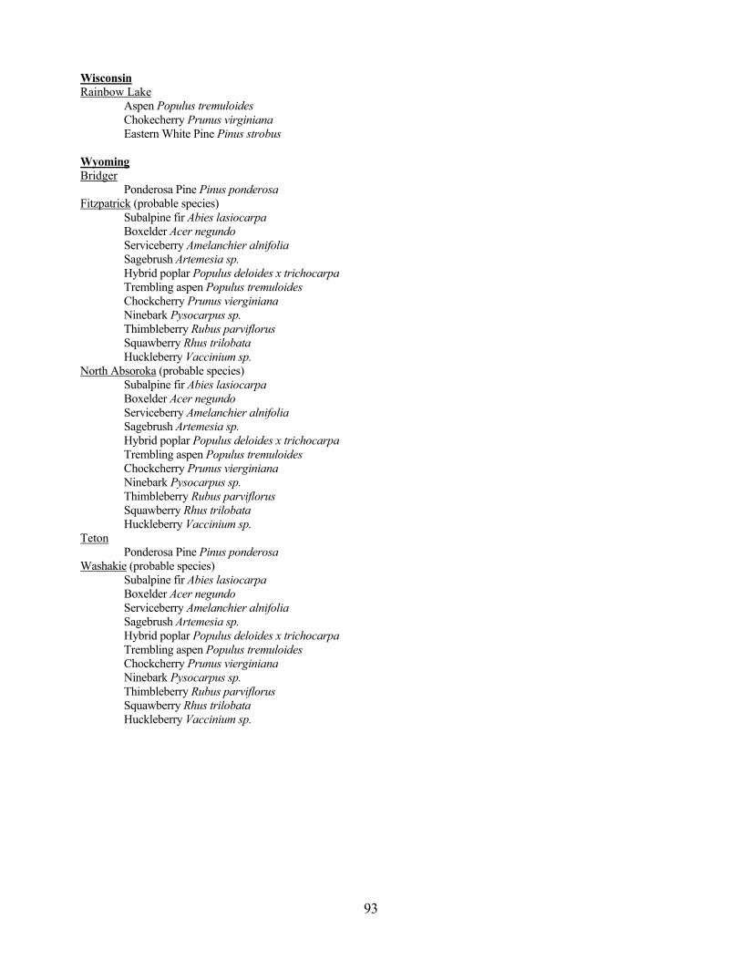
93

Wisconsin Rainbow Lake

Aspen Populus tremuloides Chokecherry Prunus virginiana Eastern White Pine Pinus strobus

Wyoming Bridger Ponderosa Pine Pinus ponderosa Fitzpatrick (probable species) Subalpine fir Abies lasiocarpa Boxelder Acer negundo Serviceberry Amelanchier alnifolia Sagebrush Artemesia sp.

Hybrid poplar Populus deloides x trichocarpa Trembling aspen Populus tremuloides

Chockcherry Prunus vierginiana Ninebark Pysocarpus sp.

Thimbleberry Rubus parviflorus Squawberry Rhus trilobata Huckleberry Vaccinium sp. North Absoroka (probable species) Subalpine fir Abies lasiocarpa Boxelder Acer negundo Serviceberry Amelanchier alnifolia Sagebrush Artemesia sp.



Thimbleberry Rubus parviflorus Squawberry Rhus trilobata Huckleberry Vaccinium sp. Teton Ponderosa Pine Pinus ponderosa Washakie (probable species) Subalpine fir Abies lasiocarpa Boxelder Acer negundo Serviceberry Amelanchier alnifolia Sagebrush Artemesia sp.



Thimbleberry Rubus parviflorus Squawberry Rhus trilobata Huckleberry Vaccinium sp.

94

2. NPS CLASS I AREAS Alaska Denali NP Quaking aspen Populus tremuloides Black poplar Populus balsamifera Arizona Chiricahua NM Arizona pine Pinus ponderosa Skunkbush Rhus trilobata White stem blazingstar Mentzelia albicaulis Black cherry Prunus serotina White clover Trifolium repens Grand Canyon NP Cottonwood Populus fremontii Ponderosa pine Pinus ponderosa Quaking aspen Populus tremuloides Single-leaf ash Fraxinus anomala Skunkbush Rhus trilobata Serviceberry Amelanchier alnifolia White stem blazingstar Mentzelia albicaulis Smooth desert dandelion Malacothrix glabrata Desert dandelion Malacothrix glabrata White clover Trifolium repens Petrified Forest NP Skunkbush Rhus trilobata Cheat grass Bromus tectorum Red-stem stork’s bill Erodium cicutarium Perrenial rye grass Lolium perenne White stem blazingstar Mentzelia albicaulis Saguaro NP Ponderosa pine Pinus ponderosa Skunkbush Rhus trilobata Quaking aspen Populus tremuloides California Joshua Tree NP Single-leaf ash Fraxinus anomala Skunkbush Rhus trilobata White stem blazingstar Mentzelia albicaulis Kings Canyon NP Jeffrey pine Pinus jeffreyi Ponderosa pine Pinus ponderosa Twinberry Lonicera involucrata Quaking aspen Populus tremuloides Chokecherry Prunus virginiana Skunkbush Rhus trilobata Butterweed groundsel Senecio serra White clover Trifolium repens Black poplar Populus balsamifera trichocarpa Lassen Volcanic NP Skunkbush Rhus trilobata Chokecherry Prunus virginiana Ponderosa pine Pinus ponderosa White clover Trifolium repens Jeffrey pine Pinus jeffreyi

95

Lava Beds NM Chokecherry Prunus virginiana Ponderosa pine Pinus ponderosa Quaking aspen Populus tremuloides Jeffrey pine Pinus jeffreyi Point Reyes National Seashore Ledebour’s honeysuckle Lonicera involucrata White clover Trifolium repens Redwood NP White clover Trifolium repens Black poplar Populus balsamifera trichocarpa Chokecherry Prunus virginiana Jeffrey pine Pinus jeffreyi Sequoia NP Jeffrey pine Pinus jeffreyi Ponderosa pine Pinus ponderosa Twinberry Lonicera involucrata Quaking aspen Populus tremuloides Chokecherry Prunus virginiana Skunkbush Rhus trilobata Butterweed groundsel Senecio serra White clover Trifolium repens Black poplar Populus balsamifera trichocarpa Yosemite NP Ponderosa pine Pinus ponderosa White clover Trifolium repens Skunkbush Rhus trilobata Twinberry honeysuckle Lonicera involucrata Chokecherry Prunus virginiana Colorado Black Canyon of the Gunnison NP Serviceberry Amelanchier alnifolia Quaking aspen Populus tremuloides Skunkbush Rhus trilobata White clover Trifolium repens Chokecherry Prunus virginiana Great Sand Dunes NM Ponderosa pine Pinus ponderosa Quaking aspen Populus tremuloides Serviceberry Amelanchier alnifolia Mountain ninebark Physocarpus monogynus Skunkbush Rhus trilobata White stem blazingstar Mentzelia albicaulis White clover Trifolium repens Mesa Verde NP

Ponderosa pine Pinus ponderosa Spreading dogbane Apocynum androsaemifolium Box elder Acer negundo Cheat grass Bromus tectorum Poison ivy Toxicodendron radicans Skunkbush Rhus trilobata

Serviceberry Amelanchier alnifolia Quaking aspen Populus tremuloides White stem blazingstar Mentzelia albicaulis White clover Trifolium repens

96

Rocky Mountain NP Wild strawberry Fragaria virginiana Mountain ninebark Physocarpus monogyna Ponderosa pine Pinus ponderosa Balsam poplar Populus balsamifera Quaking aspen Populus tremuloides Chokecherry Prunus virginiana White clover Trifolium repens Hawaii Haleakala NP Ponderosa pine Pinus ponderosa White clover Trifolium repens Hawaii Volcanoes NP White clover Trifolium repens Idaho Craters of the Moon NM Black poplar Populus balsamifera trichocarpa Quaking aspen Populus tremuloides Kentucky Mammoth Cave NP Yellow-poplar Liriodendron tulipifera Red maple Acer rubrum Poke milkweed Asclepias exaltata American sycamore Platanus occidentalis Black cherry Prunus serotina Black-eyed susan Rudbeckia hirta Cutleaf coneflower Rudbeckia laciniata Sassafras Sassafras albidum Green ash Fraxinus pennsylvanica White clover Trifolium repens Maine Acadia NP Broad-leaf aster Aster macrophyllus Black cherry Prunus serotina Quaking aspen Populus tremuloides White ash Fraxinus americana Spreading dogbane Apocynum androsaemiolium Michigan Isle Royale NP Common snowberry Symphoricarpos albus Quaking aspen Populus tremuloides Twinberry honeysuckle Lonicera involucrata Black poplar Populus balsamifera White clover Trifolium repens Red maple Acer rubrum Chokecherry Prunus virginiana Bigleaf aster Aster macrophyllus Paper birch Betula papyrifera

97

Minnesota Voyageurs NP Green ash Fraxinus pennsylvanica Quaking aspen Populus tremuloides Chokecherry Prunus virginiana White clover Trifolium repens Snowberry Symphoricarpos albus Paper birch Betula papyrifera Common milkweed Asclepias syriaca Black poplar Populus balsamifera Red maple Acer rubrum Montana Glacier NP Paper birch Betula papyrifera Wild strawberry Fragaria virginiana Twinberry Lonicera involucrata Rock-spiraea Holodiscus discolor Ponderosa pine Pinus ponderosa Black poplar Populus balsamifera trichocarpa Quaking aspen Populus tremuloides Chokecherry Prunus virginiana Snowberry Symphoricarpos albus White clover Trifolium repens New Mexico Bandelier NM Ponderosa pine Pinus ponderosa Quaking aspen Populus tremuloides Skunkbush Rhus trilobata White clover Trifolium repens Carlsbad Caverns NP Ponderosa pine Pinus ponderosa Fremont’s cottonwood Populus fremontii Quaking aspen Populus tremuloides White stem blazingstar Mentzelia albicaulis Black cherry Prunus serotina North Carolina/Tennessee Great Smoky Mountains NP Yellow-poplar Liriodendron tulipifera Red maple Acer rubrum Tall milkweed Asclepias exaltata Table-mountain pine Pinus pungens American sycamore Platanus occidentalis Black cherry Prunus serotina Winged sumac Rhus copallina Black-eyed susan Rudbeckia hirta Cutleaf coneflower Rudbeckia laciniata Crown-beard Verbesina occidentalis Sassafras Sassafras albidum

98

North Dakota Theodore Roosevelt NP Paper birch Betula papyrifera Wild strawberry Fragaria virginiana Ponderosa pine Pinus ponderosa Quaking aspen Populus tremuloides Chokecherry Prunus virginiana White clover Trifolium repens Oregon Crater Lake NP Ponderosa pine Pinus ponderosa Black poplar Populus balsamifera trichocarpa Quaking aspen Populus tremuloides Lodgepole pine Pinus contorta South Dakota Badlands NP Green ash Fraxinus pennsylvanica Ponderosa pine Pinus ponderosa Chokecherry Prunus virginiana Snowberry Symphoricarpos albus Western wormwood Artemisia ludoviciana Wind Cave NP Wild strawberry Fragaria virginiana Green ash Fraxinus pennsylvanica Quaking aspen Populus tremuloides Ponderosa pine Pinus ponderosa Chokecherry Prunus virginiana Texas Big Bend NP Ponderosa pine Pinus ponderosa Quaking aspen Populus tremuloides Black cherry Prunus serotina Skunkbush Rhus trilobata Guadalupe Mountains NP Ponderosa pine Pinus ponderosa Quaking aspen Populus tremuloides Black cherry Prunus serotina White stem blazingstar Mentzelia albicaulis Chokecherry Prunus virginiana Utah Arches NP Cottonwood Populus fremontii Single-leaf ash Fraxinus anomala Skunkbush Rhus trilobata White stem blazingstar Mentzelia albicaulis Bryce Canyon NP Ponderosa pine Pinus ponderosa Quaking aspen Populus tremuloides Skunkbush Rhus trilobata White clover Trifolium repens

99

Canyonlands NP Cottonwood Populus fremontii Single-leaf ash Fraxinus anomala Serviceberry Amelanchier alnifolia Quaking aspen Populus tremuloides White stem blazingstar Mentzelia albicaulis Capitol Reef NP Ponderosa pine Pinus ponderosa Quaking aspen Populus tremuloides Cottonwood Populus fremontii Single-leaf ash Fraxinus anomala Serviceberry Amelanchier alnifolia Skunkbush Rhus trilobata White stem blazingstar Mentzelia albicaulis White clover Trifolium repens Smooth desert dandelion Malacothrix glabrata Zion NP Cottonwood Populus fremontii Ponderosa pine Pinus ponderosa Quaking aspen Populus tremuloides Skunkbush Rhus trilobata Serviceberry Amelanchier alnifolia White stem blazingstar Mentzelia albicaulis White clover Trifolium repens Virginia Shenandoah NP Black cherry Prunus serotina Quaking aspen Populus tremuloides White ash Fraxinus americana Common milkweed Asclepias syriaca Yellow-poplar Liriodendron tulipifera American sycamore Platanus occidentalis White clover Trifolium repens Washington Mount Rainier NP Ponderosa pine Pinus ponderosa Black poplar Populus balsamifera trichocarpa Quaking aspen Populus tremuloides Twinberry Lonicera involucrata Serviceberry Amelanchier alnifolia Snowberry Symphoricarpos albus North Cascades NP Ponderosa pine Pinus ponderosa Black poplar Populus balsamifera trichocarpa Paper birch Betula papyrifera Box elder Acer negundo Twinberry Lonicera involucrata Serviceberry Amelanchier alnifolia Snowberry Symphoricarpos albus Olympic NP Black poplar Populus balsamifera trichocarpa Twinberry Lonicera involucrata Serviceberry Amelanchier alnifolia Snowberry Symphoricarpos albus

100

Wyoming Grand Teton NP Wild strawberry Fragaria virginiana Twinberry Lonicera involucrata Black poplar Populus balsamifera trichocarpa Quaking aspen Populus tremuloides Chokecherry Prunus virginiana Skunkbush Rhus trilobata Bitterweed groundsel Senecio serra White clover Trifolium repens Yellowstone NP Wild strawberry Fragaria virginiana Twinberry Lonicera involucrata White stem blazingstar Mentzelia albicaulis Black poplar Populus balsamifera trichocarpa Quaking aspen Populus tremuloides Chokecherry Prunus virginiana Skunkbush Rhus trilobata Butterweed groundsel Senecio serra White clover Trifolium repens

101

3. FWS CLASS I WILDERNESS AREAS Florida Chassahowitzka Eastern redbud Cercis canadensis Sweetgum Liquidambar styraciflua Loblolly pine Pinus taeda Black cherry Prunus serotina Dwarf sumac Rhus copallina Blackeyed Susan Rudbeckia hirta Georgia Okefenokee American sycamore Platanus occidentalis Black cherry Prunus serotina Dwarf sumac Rhus copallina Eastern poison ivy Toxicodendron radicans Eastern redbud Cercis canadensis Flowering dogwood Cornus florida Loblolly pine Pinus taeda Red maple Acer rubrum Sweetgum Liquidambar styraciflua Tree-of-heaven Ailanthus altissima Virginia creeper Parthenocissus quinquefolia Maine Moosehorn Spreading dogbane Apocynum androsaemifolium Swamp milkweed Asclepias incarnata Whorled wood aster Aster acuminatus Bigleaf aster Aster macrophyllus Parasol aster Aster umbellatus White ash Fraxinus americana Green ash Fraxinus pennsylvanica Quaking aspen Populus tremuloides Pin cherry Prunus pennsylvanica Black cherry Prunus serotina

Common chokecherry Prunus virginiana Staghorn sumac Rhus typhina Allegheny blackberry Rubus allegheniensis American elder Sambucus canadensis Michigan Seney American basswood Tilia americana Bigleaf aster Aster macrophyllus Blackeyed Susan Rudbeckia hirta Common milkweed Asclepias syriaca Eastern poison ivy Toxicodendron radicans Quaking aspen Populus tremuloides Red maple Acer rubrum Sambucus nigra Sambucus canadensis Scarlet elderberry Sambucus racemosa Spreading dogbane Apocynum androsaemifolium

102

Missouri Mingo Tuliptree Liriodendendron tulipifera Virginia creeper Parthenocissus quinquefolia Montana Medicine Lake Cheatgrass Bromus tectorum Quaking aspen Populus tremuloides White ash Fraxinus americana New Jersey Brigantine Boxelder Acer negundo Tree-of-heaven Ailanthus altissima Common milkweed Asclepias syriaca Cheatgrass Bromus tectorum Sweet gum Liquidambar styraciflua Virginia creeper Parthenocissus quinquefolia Pitch pine Pinus rigida

Black cherry Prunus serotina Winged sumac Rhus copallina American elder Sambucus canadensis Sassafras Sassafras albidum

Common lilac Syringa vulgaris Poison-ivy Toxicodendron radicans Grape Vitis spp.

North Dakota Lostwood Boxelder Acer negundo Quaking aspen Populus tremuloides Raspberry Rubus idaeus Saskatoon serviceberry Amelanchier alnifolia Oklahoma Wichita Mountains Blackeyed Susan Rudbeckia hirta Cheatgrass Bromus tectorum Eastern redbud Cercis canadensis Green ash Fraxinus pennsylvanica Smooth sumac Rhus glabra Sugar Maple Acer saccharum Virginia creeper Parthenocissus quinquefolia South Carolina Cape Romain Sweetgum Liquidambar styraciflua Virginia creeper Parthenocissus quinquefolia

Winged sumac Rhus copallina American elder Sambucus canadensis Chinese tallow tree Sapium sabiferum Poison-ivy Toxicodendron radicans Labrusca grape Vitis labrusca

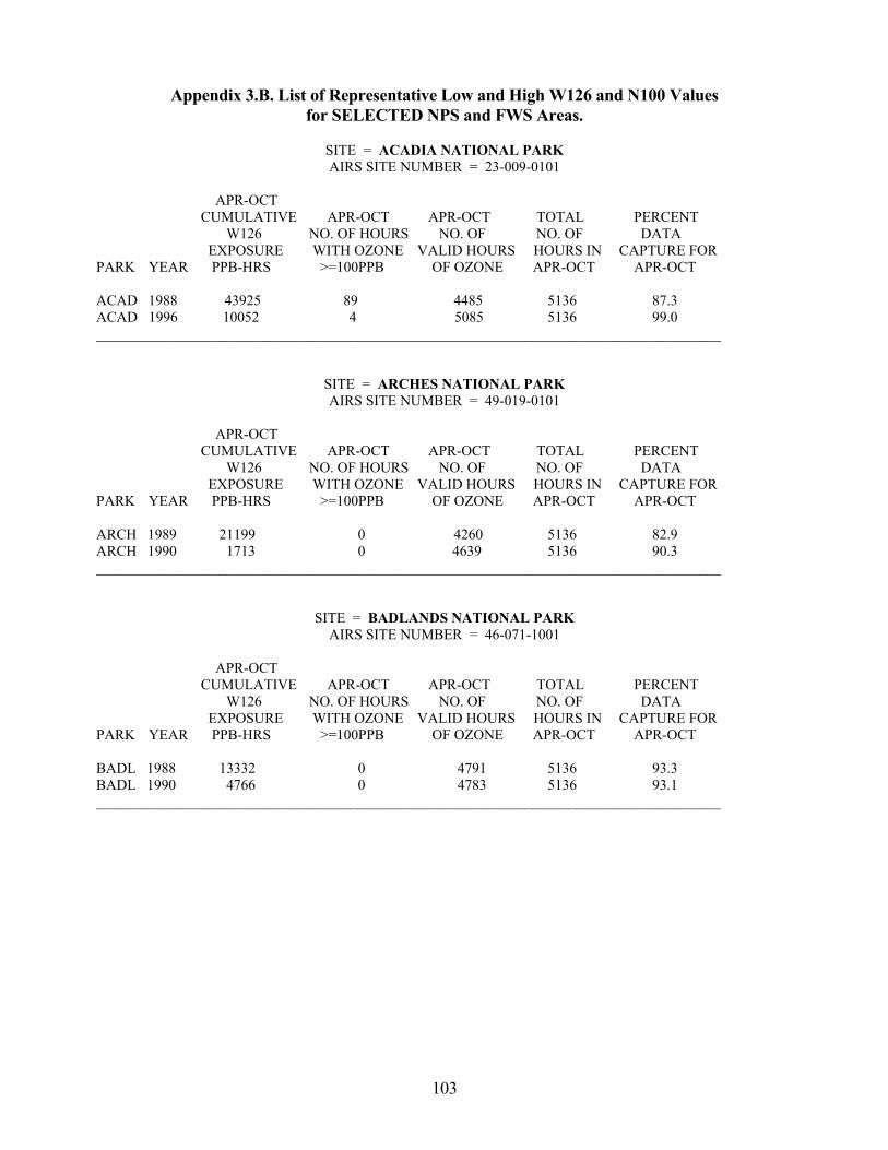
103

Appendix 3.B. List of Representative Low and High W126 and N100 Values for SELECTED NPS and FWS Areas.

SITE = ACADIA NATIONAL PARK AIRS SITE NUMBER = 23-009-0101

APR-OCT

CUMULATIVE APR-OCT APR-OCT TOTAL PERCENT W126 NO. OF HOURS NO. OF NO. OF DATA EXPOSURE WITH OZONE VALID HOURS HOURS IN CAPTURE FOR

PARK YEAR PPB-HRS >=100PPB OF OZONE APR-OCT APR-OCT ACAD 1988 43925 89 4485 5136 87.3 ACAD 1996 10052 4 5085 5136 99.0 ______________________________________________________________________________________

SITE = ARCHES NATIONAL PARK AIRS SITE NUMBER = 49-019-0101

APR-OCT


PARK YEAR PPB-HRS >=100PPB OF OZONE APR-OCT APR-OCT ARCH 1989 21199 0 4260 5136 82.9 ARCH 1990 1713 0 4639 5136 90.3 ______________________________________________________________________________________

SITE = BADLANDS NATIONAL PARK AIRS SITE NUMBER = 46-071-1001

APR-OCT


PARK YEAR PPB-HRS >=100PPB OF OZONE APR-OCT APR-OCT BADL 1988 13332 0 4791 5136 93.3 BADL 1990 4766 0 4783 5136 93.1 ______________________________________________________________________________________

104

SITE = BANDELIER NATIONAL MONUMENT AIRS SITE NUMBER = 35-028-1002

APR-OCT


PARK YEAR PPB-HRS >=100PPB OF OZONE APR-OCT APR-OCT BAND 1991 44945 0 4997 5136 97.3 BAND 1993 21854 0 4566 5136 88.9 _____________________________________________________________________________________

SITE = BIG BEND NATIONAL PARK AIRS SITE NUMBER = 48-043-0101

APR-OCT


PARK YEAR PPB-HRS >=100PPB OF OZONE APR-OCT APR-OCT BIBE 1992 12169 0 4366 5136 85.0 BIBE 1994 26667 0 4702 5136 91.5 ______________________________________________________________________________________

SITE = BIG THICKET NATIONAL PRESERVE AIRS SITE NUMBER = 48-457-0101

APR-OCT


PARK YEAR PPB-HRS >=100PPB OF OZONE APR-OCT APR-OCT BITH 1987 21554 16 4401 5136 85.7 BITH 1991 6763 1 3383 5136 65.9 ______________________________________________________________________________________

SITE = BRIGANTINE WILDERNESS AREA AIRS SITE NUMBER = 34-001-0005

APR-OCT


PARK YEAR PPB-HRS >=100PPB OF OZONE APR-OCT APR-OCT BRIG 1991 67729 109 4963 5136 96.6 BRIG 1994 24901 2 4980 5136 97.0 ______________________________________________________________________________________

105

SITE = CANYONLANDS NATIONAL PARK AIRS SITE NUMBER = 49-037-0101

APR-OCT


PARK YEAR PPB-HRS >=100PPB OF OZONE APR-OCT APR-OCT CANY 1993 21278 0 4390 5136 85.5 CANY 1996 49676 0 4373 5136 85.1 ______________________________________________________________________________________

SITE = CAPE COD NATIONAL SEASHORE AIRS SITE NUMBER = 25-001-0002

APR-OCT


PARK YEAR PPB-HRS >=100PPB OF OZONE APR-OCT APR-OCT CACO 1988 70427 174 4856 5136 94.5 CACO 1993 23439 10 4675 5136 91.0 ______________________________________________________________________________________

SITE = CAPE ROMAIN WILDERNESS AREA AIRS SITE NUMBER = 45-019-0046

APR-OCT


PARK YEAR PPB-HRS >=100PPB OF OZONE APR-OCT APR-OCT CARO 1991 4377 0 4943 5136 96.2 CARO 1993 19019 0 4945 5136 96.3 ______________________________________________________________________________________

SITE = CHAMIZAL NATIONAL MEMORIAL AIRS SITE NUMBER = 48-141-0044

APR-OCT


PARK YEAR PPB-HRS >=100PPB OF OZONE APR-OCT APR-OCT CHAM 1993 5310 1 4549 5136 88.6 CHAM 1995 19564 14 4890 5136 95.2 ______________________________________________________________________________________

106

SITE = CHANNEL ISLANDS NATIONAL PARK AIRS SITE NUMBER = 06-111-0006

APR-OCT


PARK YEAR PPB-HRS >=100PPB OF OZONE APR-OCT APR-OCT CHIS 1991 14943 0 3268 5136 63.6 CHIS 1992 33809 6 4549 5136 88.6 ______________________________________________________________________________________

SITE = CHIRICAHUA NATIONAL MONUMENT AIRS SITE NUMBER = 04-003-8001

APR-OCT


PARK YEAR PPB-HRS >=100PPB OF OZONE APR-OCT APR-OCT CHIR 1992 20023 0 4521 5136 88.0 CHIR 1994 36119 0 5005 5136 97.4 ______________________________________________________________________________________

SITE = COLORADO NATIONAL MONUMENT AIRS SITE NUMBER = 08-077-0600

APR-OCT


PARK YEAR PPB-HRS >=100PPB OF OZONE APR-OCT APR-OCT COLM 1987 35812 0 4418 5136 86.0 COLM 1990 12229 0 5012 5136 97.6 ______________________________________________________________________________________

SITE = CONGAREE SWAMP NATIONAL MONUMENT AIRS SITE NUMBER = 45-079-1006

APR-OCT


PARK YEAR PPB-HRS >=100PPB OF OZONE APR-OCT APR-OCT COSW 1990 25577 14 4004 5136 78.0 COSW 1994 5329 0 4221 5136 82.2 ______________________________________________________________________________________

107

SITE = COWPENS NATIONAL BATTLEFIELD AIRS SITE NUMBER = 45-021-0002

APR-OCT


PARK YEAR PPB-HRS >=100PPB OF OZONE APR-OCT APR-OCT COWP 1988 58732 69 4135 5136 80.5 COWP 1990 22474 0 4784 5136 93.1 ______________________________________________________________________________________

SITE = CRATERS OF THE MOON NATIONAL MONUMENT AIRS SITE NUMBER = 16-023-0101

APR-OCT


PARK YEAR PPB-HRS >=100PPB OF OZONE APR-OCT APR-OCT CRMO 1993 8563 0 4506 5136 87.7 CRMO 1994 25462 0 4752 5136 92.5 ______________________________________________________________________________________

SITE = CUYAHOGA VALLEY NATIONAL RECREATION AREA AIRS SITE NUMBER = 39-153-2004

APR-OCT


PARK YEAR PPB-HRS >=100PPB OF OZONE APR-OCT APR-OCT CUVA 1990 15249 15 3267 5136 63.6 CUVA 1991 39670 33 4193 5136 81.6 ______________________________________________________________________________________

SITE = DEATH VALLEY NATIONAL PARK AIRS SITE NUMBER = 06-027-0101

APR-OCT


PARK YEAR PPB-HRS >=100PPB OF OZONE APR-OCT APR-OCT DEVA 1994 68630 1 4125 5136 80.3 DEVA 1996 46223 0 4380 5136 85.3 ______________________________________________________________________________________

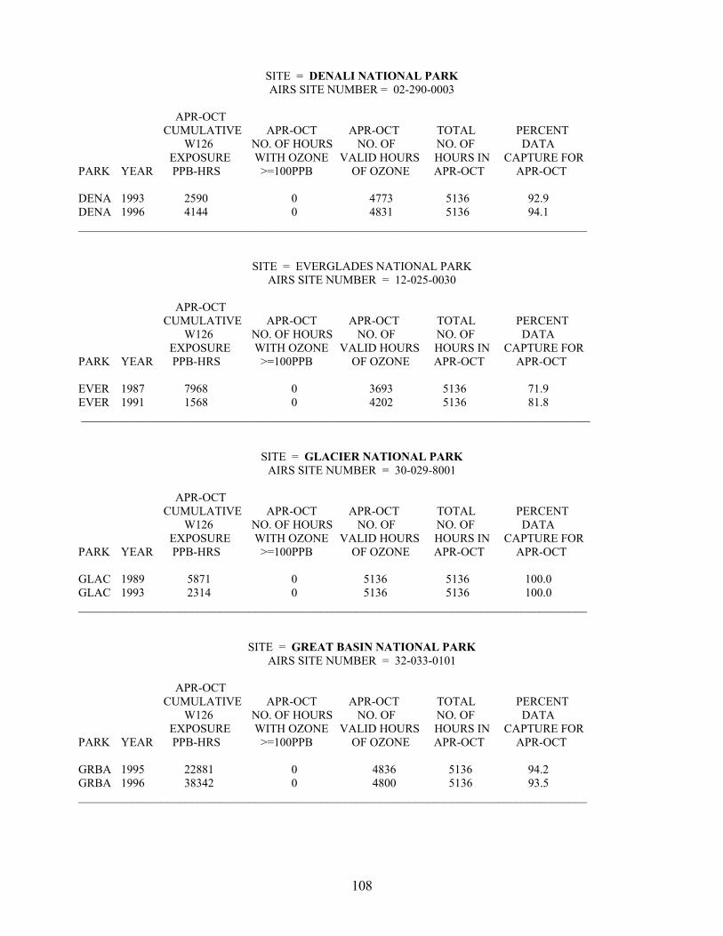
108

SITE = DENALI NATIONAL PARK AIRS SITE NUMBER = 02-290-0003

APR-OCT


PARK YEAR PPB-HRS >=100PPB OF OZONE APR-OCT APR-OCT DENA 1993 2590 0 4773 5136 92.9 DENA 1996 4144 0 4831 5136 94.1 ______________________________________________________________________________________

SITE = EVERGLADES NATIONAL PARK AIRS SITE NUMBER = 12-025-0030

APR-OCT


PARK YEAR PPB-HRS >=100PPB OF OZONE APR-OCT APR-OCT EVER 1987 7968 0 3693 5136 71.9 EVER 1991 1568 0 4202 5136 81.8 ______________________________________________________________________________________

SITE = GLACIER NATIONAL PARK AIRS SITE NUMBER = 30-029-8001

APR-OCT


PARK YEAR PPB-HRS >=100PPB OF OZONE APR-OCT APR-OCT GLAC 1989 5871 0 5136 5136 100.0 GLAC 1993 2314 0 5136 5136 100.0 ______________________________________________________________________________________

SITE = GREAT BASIN NATIONAL PARK AIRS SITE NUMBER = 32-033-0101

APR-OCT


PARK YEAR PPB-HRS >=100PPB OF OZONE APR-OCT APR-OCT GRBA 1995 22881 0 4836 5136 94.2 GRBA 1996 38342 0 4800 5136 93.5 ______________________________________________________________________________________

109

SITE = GRAND CANYON NATIONAL PARK AIRS SITE NUMBER = 04-005-2003 AND 04-005-8001

APR-OCT


PARK YEAR PPB-HRS >=100PPB OF OZONE APR-OCT APR-OCT GRCA 1990 15430 0 3827 5136 74.5 GRCA 1996 47476 0 4633 5136 90.2 ______________________________________________________________________________________

SITE = GREAT SAND DUNES NATIONAL MONUMENT AIRS SITE NUMBER = 08-003-0002

APR-OCT


PARK YEAR PPB-HRS >=100PPB OF OZONE APR-OCT APR-OCT GRSA 1989 10777 0 4436 5136 86.4 GRSA 1991 16966 0 4130 5136 80.4 ______________________________________________________________________________________

SITE = GREAT SMOKY MTS NATIONAL PARK - CADES COVE SITE AIRS SITE NUMBER = 47-009-0102

APR-OCT


PARK YEAR PPB-HRS >=100PPB OF OZONE APR-OCT APR-OCT GSCC 1994 14879 5 3988 5136 77.6 GSCC 1996 24268 0 4805 5136 93.6 ______________________________________________________________________________________

SITE = GREAT SMOKY MTS NATIONAL PARK - CLINGMANS DOME SITE AIRS SITE NUMBER = 47-155-0102

APR-OCT


PARK YEAR PPB-HRS >=100PPB OF OZONE APR-OCT APR-OCT GSCD 1993 40757 0 4087 5136 79.6 GSCD 1996 74162 3 4104 5136 79.9 ______________________________________________________________________________________

110

SITE = GREAT SMOKY MTS NATIONAL PARK - COVE MT SITE AIRS SITE NUMBER = 47-155-0101

APR-OCT


PARK YEAR PPB-HRS >=100PPB OF OZONE APR-OCT APR-OCT GSCM 1992 49135 3 4620 5136 90.0 GSCM 1996 98657 8 4879 5136 95.0 ______________________________________________________________________________________

SITE = GREAT SMOKY MTS NATIONAL PARK - LOOK ROCK SITE AIRS SITE NUMBER = 47-009-0101

APR-OCT


PARK YEAR PPB-HRS >=100PPB OF OZONE APR-OCT APR-OCT GSLR 1991 36430 0 4504 5136 87.7 GSLR 1996 76608 5 4650 5136 90.5 ______________________________________________________________________________________

SITE = GUADALUPE MOUNTAINS NATIONAL PARK AIRS SITE NUMBER = 48-109-0101

APR-OCT


PARK YEAR PPB-HRS >=100PPB OF OZONE APR-OCT APR-OCT GUMO 1990 13795 0 4531 5136 88.2 GUMO 1992 25368 0 4120 5136 80.2 ______________________________________________________________________________________

SITE = HALEAKALA NATIONAL PARK AIRS SITE NUMBER = 15-009-0101

APR-OCT


PARK YEAR PPB-HRS >=100PPB OF OZONE APR-OCT APR-OCT HALE 1992 609 0 4842 5136 94.3 HALE 1993 1197 0 4668 5136 90.9 ______________________________________________________________________________________

111

SITE = HAWAII VOLCANOES NATIONAL PARK AIRS SITE NUMBER = 15-001-0005

APR-OCT


PARK YEAR PPB-HRS >=100PPB OF OZONE APR-OCT APR-OCT HAVO 1987 3176 0 4068 5136 79.2 HAVO 1991 244 0 4775 5136 93.0 ______________________________________________________________________________________

SITE = INDIANA DUNES NATIONAL LAKESHORE AIRS SITE NUMBER = 18-127-0020

APR-OCT


PARK YEAR PPB-HRS >=100PPB OF OZONE APR-OCT APR-OCT INDU 1989 11619 0 3708 5136 72.2 INDU 1990 64667 66 3944 5136 76.8 ______________________________________________________________________________________

SITE = ISLE ROYALE NATIONAL PARK AIRS SITE NUMBER = 26-061-0101

APR-OCT


PARK YEAR PPB-HRS >=100PPB OF OZONE APR-OCT APR-OCT ISRO 1988 11169 0 2341 5136 45.6 ISRO 1991 6804 0 2631 5136 51.2 ______________________________________________________________________________________

SITE = JOSHUA TREE NATIONAL PARK AIRS SITE NUMBER = 06-065-9002 AND 06-071-9002

APR-OCT


PARK YEAR PPB-HRS >=100PPB OF OZONE APR-OCT APR-OCT JOTR 1990 57422 32 3310 5136 64.4 JOTR 1994 151025 224 4839 5136 94.2 ______________________________________________________________________________________

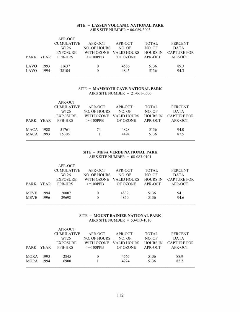
112

SITE = LASSEN VOLCANIC NATIONAL PARK AIRS SITE NUMBER = 06-089-3003

APR-OCT


PARK YEAR PPB-HRS >=100PPB OF OZONE APR-OCT APR-OCT LAVO 1993 11637 0 4586 5136 89.3 LAVO 1994 38104 0 4845 5136 94.3 ______________________________________________________________________________________

SITE = MAMMOTH CAVE NATIONAL PARK AIRS SITE NUMBER = 21-061-0500

APR-OCT


PARK YEAR PPB-HRS >=100PPB OF OZONE APR-OCT APR-OCT MACA 1988 51761 74 4828 5136 94.0 MACA 1993 15306 1 4494 5136 87.5 ______________________________________________________________________________________

SITE = MESA VERDE NATIONAL PARK AIRS SITE NUMBER = 08-083-0101

APR-OCT


PARK YEAR PPB-HRS >=100PPB OF OZONE APR-OCT APR-OCT MEVE 1994 20007 0 4832 5136 94.1 MEVE 1996 29698 0 4860 5136 94.6 ______________________________________________________________________________________

SITE = MOUNT RAINIER NATIONAL PARK AIRS SITE NUMBER = 53-053-1010

APR-OCT


PARK YEAR PPB-HRS >=100PPB OF OZONE APR-OCT APR-OCT MORA 1993 2845 0 4565 5136 88.9 MORA 1994 6900 1 4224 5136 82.2 ______________________________________________________________________________________

113

SITE = NORTH CASCADES NATIONAL PARK AIRS SITE NUMBER = 53-057-0013

APR-OCT


PARK YEAR PPB-HRS >=100PPB OF OZONE APR-OCT APR-OCT NOCA 1996 2173 0 4198 5136 81.7 ______________________________________________________________________________________

SITE = OLYMPIC NATIONAL PARK AIRS SITE NUMBER = 53-009-0012

APR-OCT


PARK YEAR PPB-HRS >=100PPB OF OZONE APR-OCT APR-OCT OLYM 1993 712 0 4585 5136 89.3 OLYM 1995 1858 0 4667 5136 90.9 ______________________________________________________________________________________

SITE = PETRIFIED FOREST NATIONAL PARK AIRS SITE NUMBER = 04-001-0012

APR-OCT


PARK YEAR PPB-HRS >=100PPB OF OZONE APR-OCT APR-OCT PEFO 1988 14446 1 4830 5136 94.0 PEFO 1989 25791 1 4696 5136 91.4 ______________________________________________________________________________________

SITE = PINNACLES NATIONAL MONUMENT AIRS SITE NUMBER = 06-069-0003

APR-OCT


PARK YEAR PPB-HRS >=100PPB OF OZONE APR-OCT APR-OCT PINN 1987 78874 86 4737 5136 92.2 PINN 1994 32951 0 4771 5136 92.9 ______________________________________________________________________________________

114

SITE = POINT REYES NATIONAL SEASHORE AIRS SITE NUMBER = 06-041-0002

APR-OCT


PARK YEAR PPB-HRS >=100PPB OF OZONE APR-OCT APR-OCT PORE 1989 4813 0 4577 5136 89.1 PORE 1990 1784 0 4856 5136 94.5 ______________________________________________________________________________________

SITE = REDWOOD NATIONAL PARK AIRS SITE NUMBER = 06-015-0002

APR-OCT


PARK YEAR PPB-HRS >=100PPB OF OZONE APR-OCT APR-OCT REDW 1988 1814 0 4825 5136 93.9 REDW 1989 1015 0 4624 5136 90.0 ______________________________________________________________________________________

SITE = ROCKY MOUNTAIN NATIONAL PARK AIRS SITE NUMBER = 08-069-0007

APR-OCT


PARK YEAR PPB-HRS >=100PPB OF OZONE APR-OCT APR-OCT ROMO 1990 5592 0 4091 5136 79.7 ROMO 1996 37033 0 4810 5136 93.7 ______________________________________________________________________________________

SITE = SAGUARO NATIONAL PARK AIRS SITE NUMBER = 04-019-0021

APR-OCT


PARK YEAR PPB-HRS >=100PPB OF OZONE APR-OCT APR-OCT SAGU 1987 9184 0 3970 5136 77.3 SAGU 1993 46792 1 4761 5136 92.7 ______________________________________________________________________________________

115

SITE = SANTA MONICA MTNS NATIONAL RECREATION AREA AIRS SITE NUMBER = 06-037-1902

APR-OCT


PARK YEAR PPB-HRS >=100PPB OF OZONE APR-OCT APR-OCT SAMO 1989 73919 238 4770 5136 92.9 SAMO 1991 63864 145 4700 5136 91.5 ______________________________________________________________________________________

SITE = SEQUOIA/KINGS CANYON NATIONAL PARKS - ASH MOUNTAIN AIRS SITE NUMBER = 06-107-0005

APR-OCT


PARK YEAR PPB-HRS >=100PPB OF OZONE APR-OCT APR-OCT SEAM 1987 165538 245 4786 5136 93.2 SEAM 1995 97343 73 4812 5136 93.7 ______________________________________________________________________________________

SITE = SEQUOIA/KINGS CANYON NATIONAL PARKS - GRANT GROVE AIRS SITE NUMBER = 06-107-0007

APR-OCT


PARK YEAR PPB-HRS >=100PPB OF OZONE APR-OCT APR-OCT SEGG 1994 135176 163 4814 5136 93.7 SEGG 1995 80484 32 4264 5136 83.0 ______________________________________________________________________________________

SITE = SEQUOIA/KINGS CANYON NATIONAL PARKS - LOWER KAWEAH AIRS SITE NUMBER = 06-107-0006

APR-OCT


PARK YEAR PPB-HRS >=100PPB OF OZONE APR-OCT APR-OCT SELK 1993 130157 137 4847 5136 94.4 SELK 1995 71759 34 4786 5136 93.2 ______________________________________________________________________________________

116

SITE = SHENANDOAH NATIONAL PARK - BIG MEADOWS AIRS SITE NUMBER = 51-113-0003

APR-OCT


PARK YEAR PPB-HRS >=100PPB OF OZONE APR-OCT APR-OCT SVBM 1988 81013 63 4448 5136 86.6 SVBM 1989 29297 0 4499 5136 87.6 ______________________________________________________________________________________

SITE = SHENANDOAH NATIONAL PARK - DICKEY RIDGE AIRS SITE NUMBER = 51-187-0002

APR-OCT


PARK YEAR PPB-HRS >=100PPB OF OZONE APR-OCT APR-OCT SVDR 1988 99239 160 3784 5136 73.7 SVDR 1992 26841 0 4351 5136 84.7 ______________________________________________________________________________________

SITE = SHENANDOAH NATIONAL PARK - SAWMILL RUN AIRS SITE NUMBER = 51-015-0042

APR-OCT


PARK YEAR PPB-HRS >=100PPB OF OZONE APR-OCT APR-OCT SVSR 1988 56538 47 4722 5136 91.9 SVSR 1989 16943 0 4490 5136 87.4 ______________________________________________________________________________________

SITE = THEODORE ROOSEVELT NATIONAL PARK - NORTH UNIT AIRS SITE NUMBER = 38-053-0002

APR-OCT


PARK YEAR PPB-HRS >=100PPB OF OZONE APR-OCT APR-OCT TRNO 1989 14184 0 4206 5136 81.9 TRNO 1993 4573 0 4281 5136 83.4 ______________________________________________________________________________________

117

SITE = VOYAGEURS NATIONAL PARK AIRS SITE NUMBER = 27-071-0101 AND 27-137-0034

APR-OCT CUMULATIVE APR-OCT APR-OCT TOTAL PERCENT

W126 NO. OF HOURS NO. OF NO. OF DATA EXPOSURE WITH OZONE VALID HOURS HOURS IN CAPTURE FOR

PARK YEAR PPB-HRS >=100PPB OF OZONE APR-OCT APR-OCT VOYA 1988 10026 3 4643 5136 90.4 VOYA 1990 2234 0 4658 5136 90.7 ______________________________________________________________________________________

SITE = YELLOWSTONE NATIONAL PARK AIRS SITE NUMBER = 56-039-1010 AND 56-039-1011

APR-OCT


PARK YEAR PPB-HRS >=100PPB OF OZONE APR-OCT APR-OCT YELL 1990 3794 0 4663 5136 90.8 YELL 1994 15212 0 4825 5136 93.9 ______________________________________________________________________________________

SITE = YOSEMITE NATIONAL PARK - CAMP MATHER AIRS SITE NUMBER = 06-109-0004

APR-OCT


PARK YEAR PPB-HRS >=100PPB OF OZONE APR-OCT APR-OCT YOCM 1989 21184 0 4321 5136 84.1 YOCM 1994 52334 0 4567 5136 88.9 ______________________________________________________________________________________

SITE = YOSEMITE NATIONAL PARK - TURTLEBACK DOME AIRS SITE NUMBER = 06-043-0003

APR-OCT


PARK YEAR PPB-HRS >=100PPB OF OZONE APR-OCT APR-OCT YOTD 1994 103128 21 4881 5136 95.0 YOTD 1995 65291 10 4467 5136 87.0 ______________________________________________________________________________________

118

SITE = YOSEMITE NATIONAL PARK - WAWONA VALLEY AIRS SITE NUMBER = 06-043-0004

APR-OCT


PARK YEAR PPB-HRS >=100PPB OF OZONE APR-OCT APR-OCT YOWV 1987 70513 44 4742 5136 92.3 YOWV 1994 27911 0 4720 5136 91.9 ______________________________________________________________________________________

SITE = YOSEMITE NATIONAL PARK - YOSEMITE VALLEY AIRS SITE NUMBER = 06-043-0005

APR-OCT


PARK YEAR PPB-HRS >=100PPB OF OZONE APR-OCT APR-OCT YOYV 1991 15175 0 4620 5136 90.0 YOYV 1994 31740 1 4780 5136 93.1 ______________________________________________________________________________________

119

4. DEPOSITION a. Introduction Atmospheric deposition has been studied extensively throughout the world, beginning in the 1800’s in England, Sweden, Norway, and Germany. Research has primarily focused on the deposition of acidic pollutants and long-term acidification. Many publications describe current conditions, monitoring and modeling methods, and the results of acidification experiments. In the United States, research on acidification was first begun in 1962 at Hubbard Brook, New Hampshire. Subsequent work in the Adirondack lakes and other areas furthered the understanding of acid deposition effects. It is now recognized that, in addition to causing acidification, deposition of pollutants can affect many ecosystem characteristics, including nutrient cycling and biological diversity. Although much progress has been made to control sulfur dioxide and nitrogen oxide emissions, deposition of sulfur (S) and nitrogen (N) compounds continues to be a problem in North America and Europe (Hedin and Likens 1996). As a result, certain sensitive freshwater lakes and streams continue to lose acid-neutralizing capacity (ANC) and sensitive soils continue to be acidified. Other ecosystems, including forests, grasslands, estuaries, and N-limited lakes exhibit unwanted fertilization and other effects from excess N deposition. Federal Land Managers (FLMs) have documented the effects of S and N deposition on many air quality related values (AQRVs). Documented effects include acidification of lakes, streams, and soils; leaching of nutrients from soils; injury to high-elevation spruce forests; changes in terrestrial and aquatic species composition and abundance; changes in nutrient cycling; unnatural fertilization of terrestrial ecosystems; and eutrophication of estuarine and some lake systems. FLMs recognize that other undocumented effects may also be occurring. The FLAG deposition subgroup was formed to identify common approaches among these agencies for evaluating atmospheric deposition and its effects on AQRVs. In addition, the subgroup was directed to recommend methods for establishing critical deposition loading values (“critical loads”) and, where possible, recommend such critical loads for specific areas. These tasks were assigned to Phase I or Phase II, depending on their degree of difficulty. During the scoping process, the FLAG Deposition Subgroup determined that Phase I tasks would include the summarization of information currently available about deposition and its effects on FLM areas and the development of recommendations on methods to model and evaluate current and future deposition and its effects on AQRVs. In addition, critical load values, where available from previous FLM guidance documents, would be referenced. FLMs agreed that site-specific AQRV and critical load information would be maintained on FLM web sites, rather than included in the Phase I report. In this way, the information can be updated and the most recent versions made quickly available to the public. Some of this information is already available on FLM web sites, and the FLMs are committed to entering remaining available information as soon as possible. The subgroup recognizes that the development and refinement of site-specific critical load values for all FLM areas are crucial for AQRV protection. However, because of the complexity of this undertaking, and the lack of information for many areas, it was deferred to Phase II.

120

During Phase II, the subgroup will focus efforts on developing methods for establishing critical deposition loading values for FLM areas, and establishing critical loads for areas with adequate information. For areas lacking sufficient information to determine critical loads, strategies will be developed to obtain needed information. Previously established critical loads will be reviewed and refined as necessary. The subgroup will also explore alternative methods for estimating background deposition rates, including extrapolation techniques or modeling that considers the spatial scale of ecosystems and differences in elevation. Methods for addressing problems with dry deposition and cloud and fog deposition measurements will also be considered. In addition, Phase II will provide research or monitoring recommendations to improve our understanding of deposition and its effects, including effects on cultural resources. b. Current Trends in Deposition From 80%-99% of S emissions and from 83%-95% of nitrogen oxides emissions are anthropogenic (NAPAP 1991). As a result, most S and N deposition is anthropogenic in origin. The Clean Air Act mandated reductions in S and N emissions that should result in decreases in S and N deposition. Deposition monitoring data can be used to identify decreases in deposition. The National Atmospheric Deposition Program (NADP) provides one of the best and most comprehensive long-term records of wet deposition chemistry in the U.S. Results from a trends analysis of 1983-1994 data from 153 NADP sites (Lynch et al. 1996) are shown on Figures D-2, D-3, and D-4. Figure D-2 shows that, between 1983-1994, wet precipitation sulfate concentrations declined significantly at 38% of monitored sites, presumably as a result of the Clean Air Act and mandated emissions reductions. Numeric declines were observed at the majority of the remaining sites. Sulfate concentrations increased significantly at only one site. A more recent analysis of 1995-1997 NADP data from eastern sites showed continuing declines in sulfate concentrations and wet depositions over much of the northeastern U.S. (Lynch et al. 2000). The EPA’s “National Air Quality and Emissions Trends Report, 1998,” also reported declines in the concentrations of sulfate in wet deposition, noting that the reductions were directly related to the large regional decreases in sulfur dioxide emissions resulting from Phase I of the Acid Rain program (U.S. EPA 2000). Despite emissions reductions, many FLM areas are located where current sulfate, and therefore total S, deposition remains high and where deposition is in excess of estimated critical loads. A workgroup convened by the Ecological Society of America (ESA) in 1999 concluded that in some regions and ecosystems, current reductions of S emissions may be insufficient for ecological recovery to occur (ESA 2000). Surface water sulfate concentrations are generally not decreasing because of the desorption of previously deposited S from soils (Johnson and Henderson 1979), and surface S mineralization with pond and lake water level changes (Schindler 1998). Elevated surface water sulfate concentrations from past deposition is expected to persist for decades even with continued emission declines. Chronic high surface water sulfate levels reduce ANC, making ecosystems more vulnerable to chemical change during episodic events. Figure D-3 shows that there is no consistent trend in nitrate concentrations. The number of sites exhibiting increasing trends is nearly equal to the number exhibiting decreasing trends. However, the number of sites that experienced a statistically significant increase in nitrate (14%) was much greater than the number of sites that experienced a significant decrease in nitrate (1.3%). Figure D-4 shows an increase in ammonium concentrations at most sites, with statistically significant increases at 22% of

121

the sites, mostly in the West. Only one site had a significant decreasing trend. Given the increases in nitrate and ammonium, total N concentrations are clearly increasing at some locations. Estimates of natural background S and N precipitation concentrations and deposition can be made from certain reliable early precipitation chemistry data (Junge 1958), precipitation data from carefully selected remote areas such as Alaska and Argentina, and to some extent from present NADP data from coastal Oregon and Alaska (NADP 1982-1997). Except for coastal Oregon, present precipitation S and N concentrations throughout the contiguous states exceed these estimates of natural background levels, primarily due to anthropogenic emissions of S and N compounds. In this chapter, it is assumed that S is deposited into the environment primarily as sulfate ion and N is deposited primarily as nitrate and ammonium ions. Other ionic forms of S and N occur in the atmosphere, but information on their deposition into ecosystems is limited. For example, organic N may be important in some areas, but reliable measurement methods for organic N in atmospheric deposition are not widely available.

122

Figure D-2. Trends in sulfate ion concentration, 1983-1994 (Lynch et al. 1996).

123

Figure D-3. Trends in nitrate ion concentration, 1983-1994 (Lynch et al. 1996).

124

Figure D-4. Trends in ammonium ion concentration, 1983-1994 (Lynch et al. 1996).

125

c. Identification and Assessment of AQRVs AQRVs sensitive to pollutant deposition have been identified in various documents published by the USDA/FS, NPS, and FWS, which are listed in the “General References” of Appendix H of this report. The FLMs have previously used a combination of approaches to identify AQRVs, including national and regional workshops, regional reviews, and site-specific studies. AQRV identification was based on information from peer-reviewed scientific literature and expert judgment. Because information on AQRVs may change as new data becomes available, the FLMs agree that AQRV information will be made available on FLM web sites to allow for updating and improve accessibility, as discussed in the Introduction to this chapter. Information on AQRVs for many USDA/FS Class I areas can be found at

http://www.fs.fed.us/r6/aq/natarm. The USDA/FS is currently adding to and updating this information. NPS and FWS are currently developing a web site with AQRV information that will be linked to the NPS AirWeb at

http://www.nature.nps.gov/ard and to the FWS National Wildlife Refuge System web site at

http://refuges.fws.gov. FLMs recommend that permit applicants consult with the appropriate FLM (Appendix F) to determine the need for an AQRV analysis and, if applicable, the methods for the analysis. All FLMs use a similar conceptual approach to identify AQRVs that reflects the FLMs’ interest in maintaining the integrity of ecosystem structure and function and protecting the most sensitive ecosystem components. AQRVs can be categorized by the type of ecosystem in which they are found, such as terrestrial, freshwater, and estuarine ecosystems. Each ecosystem and its AQRVs responds somewhat differently to deposition and approaches to evaluating deposition effects must therefore be developed accordingly. In terrestrial ecosystems, detection of changes in production, decomposition, and nutrient cycling processes provide information on deposition stress. In aquatic and estuarine ecosystems, detection of changes in water chemistry and aquatic community composition and structure provide similar information. Table D-1 summarizes AQRV indicators that may be used to assess effects in various ecosystems.

126

Table D-1. Indicators for monitoring and evaluating effects from deposition of S and N.

ECOSYSTEM INDICATORS FOR SULFUR DEPOSITION Freshwater Chemical change (ANC depression), changes in

phytoplankton and benthic community composition, species diversity, biomass

Terrestrial Leaching of soil cations, soil acidification, mobilization of aluminum ions

Estuarine Saltwater not sensitive to S deposition; leaching of nutrients may occur in sandy nearshore soils

ECOSYSTEM INDICATORS FOR NITROGEN DEPOSITION Freshwater Chemical change (ANC depression), changes in

phytoplankton and benthic community composition, species diversity, biomass

Terrestrial Changes in: litter and soil carbon and N dynamics; biomass; soil N processes; litter decomposition rates; soil microbe functional groups; soil organic matter quality and quantity; soilwater chemistry

Estuarine Changes in: phytoplankton species composition and biomass; aquatic invertebrates; seagrass health and distribution; nutrient ratios; dissolved oxygen; trophic status

Terrestrial, freshwater, and estuarine AQRVs are discussed below. In addition, methods to evaluate S- and N-induced deposition stress are discussed. Terrestrial Ecosystems Terrestrial ecosystem AQRVs include flora, fauna, and soils. FLMs have identified, where possible, AQRVs, or characteristics of AQRVs, most likely to be sensitive to S and N deposition (“sensitive receptors”). For example, high-elevation spruce forests may be sensitive receptors. FLMs assess the condition of these sensitive receptors by evaluating some aspect of the receptor (the “sensitive receptor indicator”, or “indicator”). For example, an indicator for high-elevation red spruce forests is the occurrence and extent of winter foliar injury. In general, the FLM has focused on deposition effects to vegetation and chemical receptors in terrestrial ecosystems, with little emphasis on fauna. In addition, there is increasing awareness among FLMs that certain soil fauna (e.g., microorganisms and invertebrates) are very sensitive to deposition and can be used as sensitive receptors. In terrestrial ecosystems, sulfate production is regulated primarily by chemical processes (Johnson et al. 1983) and it is rarely a limiting nutrient. Soil response to acidic deposition can be evaluated by monitoring the leaching of essential soil cations, soil acidification, and mobilization of ionic aluminum. These processes have been studied both in field and laboratory experiments, and are defined in detail in the literature (Mollitor and Raynal 1983, Richter et al. 1983, Johnson et al. 1983, Reuss and Johnson 1986). Effects of S deposition can be detected by monitoring calcium and

127

magnesium ions and S in the litter layer and surface soils; calcium, magnesium, potassium, and sulfate ions in soil solution; cation exchange capacity (CEC); and base saturation. In general, biological AQRVs do not provide reliable indicators of S deposition in terrestrial ecosystems except under extreme S deposition. Lichens have been used in some areas as biomonitors to demonstrate spatial trends in S deposition, particularly in areas with pronounced S deposition gradients. For example, isotopic analysis of lichens from Mt. Zirkel Wilderness, Colorado, indicated that power plants in the nearby Yampa Valley were the source of elevated S in the lichens (Jackson et al. 1996). Unlike S, the production and mobility of N in ecosystems is regulated almost entirely by biological processes. N is a limiting nutrient in most terrestrial and estuarine ecosystems, and is seasonally limiting in many freshwater ecosystems. Most ecosystems can retain and process significant additions of N, with resulting increases in production and changes in species diversity, biomass, and nutrient cycling. However, these changes are usually considered to be undesirable in natural ecosystems. The ability to retain and process N varies significantly depending on watershed successional status, site and fire history, soil conditions, vegetation, and other non-human factors. When N inputs exceed an ecosystem’s assimilation capacity, N is lost or leached, usually as nitrate, from the soil and can be detected in adjacent streams or lakes. This may occur following a major disturbance such as fire, logging, land use change, grazing, agriculture, or where atmospheric N deposition or experimental inputs exceed what the ecosystem can assimilate (Fenn and Dunn 1989, Fenn 1991, Fenn et al. 1996, Adams et al. 1997). Studies in northern Europe (Dise and Wright 1995) found that European forests leached detectable levels of nitrate at inputs of about 10-25 kilograms N per hectare per year (kg N ha-1yr-1). Tundra and high-elevation alpine sites may leach N at much lower levels of input. Mountain watersheds in the western U.S. show signs of N leakage at wet deposition levels of 3-5 kg N ha-1yr-1 (Eilers et al. 1994; Williams et al. 1996; Williams and Tonnessen, in review). However, even high elevation, poorly vegetated ecosystems with limited soil development can process more than 80% of the atmospheric N input before it reaches the aquatic system (Campbell et al. 1995, Kendall et al. 1995). Although nitrogen leaching has often been used as an indicator of excess N deposition, major changes occur in below- and aboveground biomass, species diversity, and nutrient cycling long before N input levels are sufficient to cause nitrate leaching (NAPAP 1993, Tilman et al. 1997, Vitousek et al. 1997). For example, with ambient deposition rates of 7-10 kg N ha-1yr-1, a Minnesota Long-Term Ecological Research (LTER) grassland study observed shifts from native, warm-season grasses to low diversity mixtures dominated by cool-season grasses and a greater than 50% decline in species richness (Wedin and Tilman 1996, Tilman et al. 1997). Significant losses in terrestrial diversity may have already occurred over extensive areas of the U.S., particularly in forest understories, shrublands, grasslands, and in soil microbial communities. Because significant ecological changes may occur before nitrate loss can be detected, more sensitive indicators than nitrate leaching are needed to evaluate N deposition effects. Such indicators include changes in carbon and N dynamics of litter and soil and biomass (Aber and Driscoll 1997, Magill et al. 1997). With knowledge of inputs and small-scale N fertilization studies, changes in soil organic matter quality and quantity in response to N deposition can be evaluated. Soil microbial communities control the quantity and quality of N available to ecosystems and may be very sensitive indicators of N deposition. Changes in soil microbe functional groups or biomass may provide good estimates of ecosystem critical loads and incremental effects. Soil N mineralization, small root growth, and carbon:nitrogen ratios of soil and microbial biomass are also sensitive to N deposition. Evidence

128

suggests that current deposition rates may alter the production of dissolved organic carbon and organic N compounds in soils, which are important nutrient and energy sources for both terrestrial and aquatic ecosystems. These could also be used as indicators of N deposition effects. However, because there are many other variables that also affect soil processes, it may be very difficult to discern effects on any soil indicators that are solely attributable to N. Freshwater Ecosystems AQRVs in freshwater ecosystems include lakes and streams and their associated flora and fauna. Sensitive receptors include water chemistry and clarity, phytoplankton, zooplankton, fish, amphibians, macroinvertebrates, and benthic organisms. Water chemistry indicators that respond to deposition include pH, ANC, conductance, cations and anions, metals, and dissolved oxygen. Physical indicators, such as water clarity, and biological indicators, including species diversity, abundance, condition factor and productivity of fish, amphibians, macroinvertebrates, and plankton can also be used to detect deposition effects in aquatic ecosystems. Much research has been done on the sensitivity of aquatic species to deposition, many of which are discussed in the 1990 National Acid Precipitation Assessment Program (NAPAP) State of Science report (NAPAP 1991a) and the 1998 NAPAP report (NAPAP 1998). Sulfur is not a limiting nutrient in freshwater ecosystems. However, there are small regions of the U.S., including some FLM areas, where a relatively high percentage of surface water is sensitive to present acidic inputs. In these areas, S deposition can cause decreases in ANC and pH. For these sensitive or low-ANC waters, the best approach to quantify S deposition effects is the procedure currently used, monitoring changes in ANC and pH. Nitrogen deposition, like S deposition, can cause episodic acidification of surface water in certain sensitive high-elevation ecosystems that have low-ANC headwater lakes and streams. Episodic acidification occurs in these areas when deposition is as low as 3-5 kg N ha-1yr-1 (Williams et al. 1996). Estuarine Ecosystems AQRV sensitive receptors in estuarine ecosystems include plankton, seagrasses, and water chemistry and clarity. Associated coastal forest and dune soils may also be useful as sensitive receptors. Water and soil nutrient concentrations, phytoplankton species composition and abundance, seagrass health, and dissolved oxygen concentrations can be used to evaluate deposition effects. In estuaries, S is not a limiting nutrient. In addition, estuarine waters are highly buffered and, therefore, not subject to acidification. However, many coastal forest and dune soils are dominated by sandy soils that are sensitive to leaching of limiting nutrients because of very low cation exchange capacity (Au 1974). Monitoring for change in estuarine areas with high S deposition should therefore focus on soil ion mobility. As soil calcium and magnesium levels are generally adequate because of deposition from marine sources, potassium is likely the only limiting nutrient subject to significant loss by sulfate leaching. The role of N in estuaries is probably the best-documented example of anthropogenic alteration with a literature record dating back to the 1950s. Production and use of fertilizers, land use changes, and fossil fuel combustion have greatly increased the available N, normally a limiting nutrient, which enters coastal waters. This has increased estuarine production and accelerated the process of

129

eutrophication. Eutrophication can result in dramatic algae blooms, anoxia, the production of toxic hydrogen sulfide gas, and species extirpation in estuarine ecosystems. Human induced eutrophication has been documented for many areas along the Atlantic and Gulf coasts, including the Chesapeake Bay, Tampa Bay, Sarasota Bay, Florida Bay, and Long Island Sound. A number of FLM areas along the Atlantic and Gulf coasts contain significant coastal waters that may be sensitive to eutrophication. Little is known about excess N effects in most of these areas, although eutrophication is well documented in Florida Bay, located in Everglades National Park. Also, recent evidence indicates that coastal waters in Chassahowitzka Wilderness (Florida) experience N-induced algal blooms (Dixon and Estevez in draft). In most coastal waters, 10-45% of the N entering the system is atmospheric, either from direct deposition to surface water or deposition to the watershed. Complete elimination of atmospheric N inputs would not entirely mitigate ecosystem change due to N because of the substantial contributions from agricultural and urban runoff. However, for most estuaries, any reduction in N input would be beneficial in restoring ecosystem structure and function. The monitoring procedures recommended, and currently used, in estuaries are similar to those used in freshwater, with emphasis on incremental changes in plankton, aquatic plant, benthic, and invertebrate community composition; species diversity, distribution, and biomass; and ecosystem trophic status. Significance of Long-Term Monitoring to Evaluate Trends and Validate Modeling Long-term monitoring is critical to evaluate trends in deposition and deposition effects. Monitoring programs should concentrate not only on areas with high past and/or present sulfate, nitrate, or ammonium deposition, but also in areas that are very sensitive to deposition and in areas where deposition is expected to increase. For selected monitoring sites, the FLM should (1) obtain ion deposition data for the site, as from NADP or CASTNet, (2) identify sensitive AQRVs and appropriate variables to monitor, (3) evaluate the present condition of the sensitive AQRVs, (4) determine the degree to which results from one site can be extrapolated to other FLM areas in the region, and lastly (5) implement a long-term monitoring program, using carefully selected variables. Long-term monitoring data are also needed to support and validate models used to predict deposition and deposition effects, including the effects of increases or decreases of S and N on ecosystems. Long term studies in both aquatic and terrestrial ecosystems such as Hubbard Brook, Lake Tahoe, and the Experimental Lakes Area have provided useful information for modeling (Bormann and Likens 1967, Holm-Hanson et al. 1976, Likens and Bormann 1977, Leonard et al. 1979, Byron and Eloranta 1984, Schindler et al. 1985, Schindler 1987, Schindler et al. 1990, Jassby et al. 1995). NAPAP and the National Science Foundation LTER program have addressed monitoring to meet modeling needs in both terrestrial and aquatic ecosystems. Data requirements to support models vary, but the quality of input data will determine the quality of a model’s predictions. Modeling is further discussed in the “Other AQRV Identification and Assessment Tools” section of this chapter. d. Determining Critical Loads Critical load is defined by FLMs as “the concentration of air pollution above which a specific deleterious effect may occur.” Critical loads have been widely accepted in Europe and Canada as a basis for negotiating control strategies for transboundary air pollution (Posch et al. 1997).

130

In Canada, researchers have estimated the critical loads of S in wet deposition necessary to protect moderately sensitive lakes in eastern provinces. That value, equivalent to 6.7 kg ha-1yr-1 of S in wet deposition, was used by Canada to argue for the U.S. to implement the Clean Air Act Amendments of 1990, which call for the initial reduction of sulfur dioxide emissions in the eastern U.S. and later from all electric utilities nationwide. With additional data on lake and stream chemistry available for sensitive systems in Nova Scotia, Ontario, and Quebec, the Canadians are now recommending a more stringent critical load, equivalent to 2.7 kg ha-1yr-1 of wet deposition S. In both European countries and in North America, attention has expanded beyond ecosystem damage caused by S deposition to ecosystem damage caused by N deposition. In some European forests, chronically high N deposition has exceeded the assimilation capacity of local ecosystems, resulting in the release of nitrate into surface waters (Dise and Wright 1995). Watersheds that are leaking nitrate into surface waters during the growing season, are referred to as "N saturated" (Aber et al. 1989). Nitrogen saturation has been linked to forest decline in Europe (Schulze 1989). Based on a set of regional N addition experiments conducted at sites in northern Europe (NITREX), Wright (1995) recommended a N critical load of less than 10 kg ha-1yr-1 to protect European forests and freshwaters from N saturation. However, this critical load does not protect ecosystems from the changes caused by N deposition prior to actual N saturation, including shifts in composition and abundance of soil fauna species and alterations in soil chemistry. In the United States, two states have attempted to set deposition standards or critical loads to protect sensitive ecosystems. In 1982, the State of Minnesota passed the Acid Deposition Control Act to limit wet sulfate deposition to 11 kg ha-1yr-1, which is equivalent to 3.7 kg S ha-1yr-1. At this sulfate level, precipitation pH was likely to remain above 4.7, which would protect lakes with ANC less than 50 microequivalents per liter (µeq l-1). This critical load was to be achieved by controls on large sources of sulfur dioxide in Minnesota. As of 1990, monitoring by state officials showed no evidence of lake acidification under the sulfur dioxide control program. However, the efficacy of this control strategy is still uncertain, because as much as 90% of the sulfate deposited in northern Minnesota may have sources outside of the state (Orr et al. 1992). In 1989, the California legislature adopted the Atmospheric Acidity Protection Act, which required the Air Resources Board (CARB) to "develop and adopt standards, to the extent supportable by scientific data, at levels which are necessary and appropriate to protect public health and sensitive ecosystems from adverse effects resulting from atmospheric acidity" (CARB 1993). An assessment of existing data identified the high elevation watersheds, surface waters, and mixed conifer forests of the Sierra Nevada and the Los Angeles Basin as sensitive ecosystems. CARB analyses suggested that appropriate standards would include a critical load value for inorganic N to protect forests, and critical loads for both N and S to protect poorly buffered lakes and streams. However, no acidity standards to protect human health or critical loads to protect ecosystems have been set in California to date. The Clean Air Act Amendments of 1990, Title IV, section 404, called on the Environmental Protection Agency (EPA) to prepare a report on the feasibility and effectiveness of setting deposition standards nationwide to protect sensitive aquatic and terrestrial resources. The completed report includes a number of modeling analyses that project the effect of reductions in both S and N deposition in areas studied during NAPAP. EPA concluded that deposition standards could not be set at this time because of 1) the lack of clearly defined policy regarding appropriate or desired goals for protecting sensitive aquatic or terrestrial resources, and 2) key scientific uncertainties, particularly regarding nitrogen watershed processes. In addition, EPA recognized that a national deposition

131

standard might be inappropriate because of differences among ecosystems. However, in response to public comments on the report, EPA stated that “Given an adequate level of monitoring and assessment data, Class I areas could serve as potential targets for standard setting activities.” (U.S. EPA 1995) Critical Loads in FLM Areas In the Clean Air Act, as amended in 1977, Congress gave FLMs an “affirmative responsibility” to protect AQRVs from the adverse effects of air pollution. Congress’ intent was, “…In cases of doubt the land manager should err on the side of protecting the air quality-related values for future generations…” (Senate Report No. 95-127, 95th Congress, 1st Session, 1977). In an effort to ensure AQRV protection, FLMs have established critical loads for many FLM areas. FLMs agree that a critical load should protect the most sensitive AQRVs within each FLM area and should be based on the best science available. As new scientific information becomes available, critical loads should be reviewed and updated. Critical loads should ensure that no unacceptable change occurs to the resource. FLMs have previously used a combination of approaches to establish critical loads, including national and regional workshops, regional reviews, and site-specific studies (see Appendix H). In all cases, the FLMs have used peer-reviewed scientific literature and expert judgment to make their decisions. For example, the NPS has established critical loads for several national parks through regional reviews that have evaluated existing information on air quality, deposition, and effects on AQRVs in national parks. For these reviews, NPS grouped parks by region and ecosystem type, including the Pacific Northwest, the Colorado Plateau, and the Rocky Mountains, and conducted an empirical assessment of the status of aquatic and terrestrial resources. An analysis of deposition effects was done, using current deposition data for S and N and effects information from field observations and research. In the Pacific Northwest region, this analysis led researchers to recommend guidelines for critical loads of S and N to protect sensitive resources, particularly low-ANC lakes, streams and ponds. These guidelines for critical loads will be available on the NPS AirWeb site in the near future at:

http://www.nature.nps.gov/ard. The FWS is also committed to establishing critical load guidelines to protect sensitive resources. These guidelines for critical loads will be available through the FWS National Wildlife Refuges site at:

http://refuges.fws.gov. The USDA/FS has conducted a series of national and regional workshops to establish critical loads and concern thresholds. In the late 1980s, the USDA/FS published prototype methods for evaluating the effects of acid deposition on AQRVs, including A Screening Procedure to Evaluate Air Pollution Effects on Class I Wilderness Areas (Fox et al. 1989) and Guidelines for Measuring the Physical, Chemical, and Biological Condition of Wilderness Ecosystems (Fox et al. 1987). Subsequently, the USDA/FS held regional workshops to develop screening procedures for new air pollutant emissions sources. These workshops were comprised of national and regional USDA/FS land managers, deposition experts from the academic and air pollution research community, and agency air quality professionals. Dependent on the workshop leadership, each regional workshop followed a slightly different process and a variety of outputs and formats resulted. However, all workshops used a collaborative process to determine S and N deposition rates that would pose a risk to the aquatic and terrestrial ecosystems protected in FLM areas, while addressing the scientific uncertainty inherent in

132

ecosystem response to acidic deposition. Critical load guidelines for many USDA/FS Class I areas are published in workshop reports (see Appendix H) and are available at:

http://www.fs.fed.us/r6/aq/natarm. The USDA/FS is currently adding to and updating this information. As resources permit, during Phase II of FLAG, the subgroup will develop methods for establishing critical deposition loading values for all FLM areas and recommend critical loads for areas where adequate information exists. For areas lacking sufficient information to determine critical loads, strategies will be developed to obtain needed information. e. Other AQRV Identification and Assessment Tools In addition to AQRV monitoring, there are several tools available to the FLM for identifying AQRVs and assessing the response of sensitive AQRVs to pollutant deposition. These include the aquatic effects expert system component of the FWS/NPS Air Synthesis, the Natural Resource Information System – Air Module (NRIS-Air), and deposition models such as the Model of Acidification of Groundwater in Catchments (MAGIC) and MAGIC-With Aggregated Nitrogen Dynamics (MAGIC-WAND). Air Synthesis Air Synthesis is an information management and decision-support computer system under development by NPS and FWS. Air Synthesis is designed to assist FLMs in determining potential effects of pollutants on AQRVs. It contains information on air quality and its effects in parks and wildernesses as well as natural resource data and annotated bibliographies of current literature on deposition. An interactive expert system module is under development for inclusion in Air Synthesis to allow FLMs to assess the current status of freshwaters and determine if these resources are likely to be affected by deposition of S or N. The aquatic effects expert system is being developed by regional scientists. This system will allow FLMs to input existing surface water data for lakes and streams to determine: (1) the acidification status of the waters, (2) the likely cause of high concentrations of acid anions (e.g., deposition, land use, organic inputs) and, (3) the sensitivity of the waters to increases in N or S deposition. Results can be displayed in a geographic information system (GIS) image that color-codes the acidification status of lakes and streams. In addition, the expert system evaluates the completeness and the amount of uncertainty in water chemistry data sets. Air Synthesis will be available through the NPS AirWeb at:

http://www.nature.nps.gov/ard

or the FWS National Wildlife Refuge System web site at:

http://refuges.fws.gov. Natural Resource Information System – Air Module (NRIS-Air) The Air Module is part of the USDA/FS Natural Resource Information System that integrates various physical, biological and socioeconomic data within a system of database, map-based spatial information, and analytical tools. Version 1.0 of NRIS-Air, released in November 1998, tracks

133

AQRVs, sensitive receptors and indicators for each of the USDA/FS Class I areas. The water submodule provides data storage, reports, and tools for evaluating locally entered water quality and wet deposition data. It also integrates the NADP data set and the entire National Surface Water Survey including the Eastern and Western Lakes Surveys and the National Stream Survey. Future NRIS-Air versions under development will provide the information structure for visibility, flora, fauna, soil, geologic resources, cultural resources, and air quality data, as well as providing an air pollution permit tracking system. Information from NRIS-Air, including USDA/FS Class I area AQRV information, is available at: http://www.fs.fed.us/r6/aq/natarm. Deposition Effects Models A number of watershed process models have been developed and tested in an attempt to simulate the effects of S and N on soils, forests, and surface waters. These models are used by FLMs to predict effects from increases in deposition and vary from detailed, compartment models of watersheds to lumped parameter models that do not track different ions through each soil compartment. For a review of models developed under NAPAP see NAPAP 1991. A commonly applied watershed model is MAGIC. MAGIC was first developed for eastern U.S. watersheds and then extensively tested and validated throughout Europe and North America (Cosby et al. 1985, 1995, 1996). The model was used by NAPAP in its 1990 Integrated Assessment to project surface water chemistry resulting from various deposition scenarios (NAPAP 1991b). In another application in the eastern U.S., MAGIC has been linked with a simple, empirical, dose/response fish model developed at University of Virginia, that makes it possible to predict changes in fish productivity based on modeled changes in streamwater chemistry. As a result of NAPAP, there was increased awareness of the potential impacts of inorganic N deposition on watersheds and surface waters. In response, the MAGIC model was updated with a module called With Aggregated Nitrogen Dynamics (WAND). MAGIC-WAND is a process-based model that uses site-specific information on hydrology, soils, and hydrochemistry. The model predicts changes through time in lake or stream chemistry. These time-series of changes in pH and ANC can subsequently be used by FLMs to calculate critical S or N loads for watersheds. MAGIC-WAND has been extensively tested in the Adirondacks and at watersheds in Maine. For example, the Bear Brook Watershed Manipulation Project uses MAGIC-WAND to predict the effects of experimentally added N and S on a test watershed. MAGIC-WAND has also been applied to watersheds in FLM areas in the Cascades, the Sierra Nevada, the Rocky Mountains, and the Wind River Range in an effort to quantify critical S and N loads to aquatic and terrestrial resources. In the southeastern U.S., MAGIC-WAND is being used under the auspices of the Southern Appalachian Mountains Initiative (SAMI) to predict the effects of future deposition scenarios on FLM areas. Future SAMI modeling efforts will link watershed model results with fish dose/response models. The ultimate goal is to calibrate MAGIC-WAND with landscape level data in order to set regional critical loads. Other models are also in use. For example, the USDA/FS Rocky Mountain Region recommends using either CALPUFF or ISCST (or other approved models) to estimate S and N deposition. The Screening Methodology for Calculating ANC Change to High Elevation Lakes (USDA Forest Service

134

2000) summarizes procedures for estimating total deposition of S and N. The document also recommends computations for estimating alkalinity changes in lakes caused by increases in S and N deposition. Another model, the Nutrient Cycling Model (NuCM) has been used in the East to predict the effect of changes in deposition on nutrient concentrations in soils and vegetation. f. Recommendations and Guidance for Evaluating Potential Effects from Proposed Increases in Deposition to an FLM Area FLMs often request that proponents of new emissions sources or modifications of existing sources near FLM areas provide sufficient information for the FLM to evaluate the potential effects of emissions increases on AQRVs. FLMs have provided guidance for applicants through guidance documents, correspondence, meetings, and phone consultations. This chapter summarizes current guidance for the evaluation of new emissions on deposition and sensitive AQRVs and includes recommendations for: • the types of data, information, and analysis needed before a permit can be considered complete,

including analytical and modeling protocols for a proponent’s use in conducting an AQRV impact analysis;

• approaches and sources of appropriate values for estimating wet and dry deposition; and • permit conditions to mitigate source impacts. These recommendations can most easily be described using a flow chart. Figure D-1 summarizes the approaches to be taken to evaluate a proposed action.

135

No/Unknown

Yes

START

Current adverse

effects to AQRVsfrom deposition/

Critical load exceeded

?

Yes

Unknown

No

New emissions

cause or contribute to adverse effects/Critical

load exceeded?

FLM may recommendelements of "a" or "b"or (if necessary) "c"

a. The applicant should use one or more of the following: - Stricter (than BACT) controls (e.g., Lowest Achievable Emission Rate [LAER]). - Emission offsets located in an area that, considering geographic and meteorological factors, will benefit the impacted wilderness or park, as demostrated by modeling. - Regional modeling to identify sources contributing significantly to deposition adverse effects; SIP revision to reduce emissions contributing to adverse effects. (See text for discussion of mitigation options.) b. Deposition and deposition effects monitoring/research in the FLM area. c. Denial of permit.

FLM unlikely to object to permit

FLM unlikely toobject to permit;

may recommend "b"

Figure D-1. FLM resonse to potential deposition effects from new emissions sources.

Figure D-1. FLM response to potential deposition effects from new emissions sources.

136

The flowchart begins with the question, “Are there currently adverse effects from pollutant deposition to AQRVs in the FLM area?” To answer this question, the FLM needs information on deposition-sensitive AQRVs, deposition loads at which these AQRVs are affected (i.e., critical loads), and the current pollutant deposition rates in the area. In areas where no information is available, information from a nearby, or ecologically similar area, may be used. An adverse effect may be expected to occur if the critical load is exceeded for an area. AQRV and critical load information are discussed earlier in this report. Procedures for estimating current pollutant deposition rates are summarized in the section, “Estimation of Current and Future Deposition Rates.” After considering this information, the FLM determines if adverse effects to AQRVs already exist at an area. If adverse effects are present, the FLM may recommend that “a” or “b” or both of Figure D-1 are included as permit conditions. If these recommendations, or some combination of them, cannot be implemented, the FLM is likely to recommend denial of the permit. If there are no current documented adverse effects from pollutant deposition to AQRVs, or there is a lack of information on deposition and deposition effects in the area (and information from nearby or ecologically similar areas is unavailable), the FLM may ask, “Will the proposed action cause an adverse effect to AQRVs?” The information needed to answer this question includes the information listed above regarding AQRVs, critical loads, and current deposition rates. In addition, an estimate is needed of the future predicted deposition rate. Procedures for this estimate are found in the “Estimation of Current and Future Deposition Rates” section of this report. With this information, the FLM can determine if the proposed action is likely to cause an adverse effect to AQRVs. If the answer is no, or unknown, the FLM would not object to the action because of potential deposition effects. The FLM may still, however, object to the action for other reasons including an inadequate best available control technology analysis, predicted National Ambient Air Quality Standards violations, predicted Class I increment impacts, or other predicted AQRV impacts. If the available information is insufficient for the FLM to determine if the proposed action will cause an adverse effect to AQRVs, the FLM may ask for deposition and deposition effects monitoring and/or research in the FLM area (i.e., item “b”). If the answer is yes and the proposed action will likely cause an adverse effect to AQRVs, the FLM may recommend permit conditions that ensure mitigation, including stricter emissions controls and effective emissions offsets (i.e., item “a”). If no mitigation is possible, the FLM is likely to recommend denial of the permit. Available Deposition Monitoring Data Atmospheric pollutants are deposited to ecosystems primarily through wet deposition and dry deposition. FLMs participate in national monitoring programs to monitor wet and dry deposition, including the National Atmospheric Deposition Program (NADP) and the Clean Air Status and Trends Network (CASTNet). A 1999 report, “The Role of Monitoring Networks in the Management of the Nation’s Air Quality,” (CENR, 1999) identified these two networks as being critical for characterizing baseline air quality data in the U.S. Wet Deposition Wet deposition includes rain, snow, fog, cloudwater, and dew. In most FLM areas, rain and snow are the primary contributors to wet deposition. However, in some high elevation areas, fog, cloudwater, and dew are significant contributors, as discussed below.

Because rain and snow are the primary constituents of wet deposition at most FLM areas, the FLM generally relies on data from NADP to evaluate wet deposition of pollutants. NADP samplers collect

137

rain and snow and NADP has documented deposition for many years in a nationwide network that currently includes over 220 monitoring sites. The network collects data to evaluate spatial and temporal long-term trends in precipitation chemistry. The precipitation at each site is collected weekly and sent to a central analytical laboratory for analysis of hydrogen (acidity as pH), sulfate, nitrate, ammonium, chloride, and base cations, including calcium, magnesium, potassium, and sodium. Data and isopleth maps of pollutant concentrations and deposition are available on the NADP web site at:

http://nadp.sws.uiuc.edu/

FLMs agree that it is preferable to obtain NADP data from the web site, rather than summarizing wet deposition data in this report. In this way, current data can be easily accessed by FLMs and the public. Approximately 50 FLM areas have NADP samplers in or immediately adjacent to them. Because some of these areas are classified as wilderness, FLMs install sampling equipment in adjacent non-wilderness areas in order to preserve the wilderness character of the area. Ambient air in these adjacent areas is considered representative of air in the wilderness area. A number of FLM areas do not have an NADP sampler in or adjacent to them. Where possible, the FLM has identified an NADP site whose data may be used to characterize deposition at the area. This information is appended to this Deposition chapter (Table D-2). Deposition rates generally increase with elevation and deposition in high-elevation areas may be difficult to characterize with data from a lower-elevation NADP site. FLM consultation may be necessary to estimate deposition in these areas. Areas that experience significant deposition from fog and cloudwater or large amounts of snow may need to use alternate sampling methods and data in addition to NADP protocols and NADP data to characterize them. Wet deposition in these areas may need to be sampled with alternate methods, including cloudwater samplers and snowpack sampling or estimated by modeling. At sites where such data or modeled estimates are available, they should be used to calculate total deposition. At mountain sites frequented by clouds and fog, deposition from clouds may equal or exceed that from precipitation. Cloud water is generally more acidic and contains higher concentrations of base cations than rain water; therefore, it can contribute significantly to total loadings of S and N (Hemmerlein and Perkins 1992). Various methods have been developed to measure deposition from cloudwater. The Mountain Acid Deposition Program (MADPro) used automated cloud water collectors to sample at three high-elevation eastern sites (Anderson et al. 1999). Forests covered by fog for significant periods of time may be especially susceptible to injury from acid deposition. Acidic cloud water has predisposed red spruce in the high elevations of the northeast U.S. Appalachians to winter injury and cumulative impacts with other biotic and abiotic stresses have caused mortality. The contribution of clouds and fog to deposition at high elevations may overshadow both deposition from precipitation and dry deposition (Hidy 1998). The U.S. EPA estimated that as a result of cloud cover, high elevation forests might experience four times the amount of total pollutant deposition as lower elevation forests without cloud cover (NAPAP 1991). High elevation lakes are also impacted by fog and clouds, as well as rain and snow. Measurements in high elevation areas that do not include all contributions to wet deposition will result in under-estimates. Modeling has been used to estimate total wet deposition in some areas. For example, the Southern Appalachian Man and the Biosphere Cooperative (as part of the Southern Appalachian Assessment) has used NADP data, topographical data, and meteorological data to model wet deposition loading at locations in the southeastern U.S.

138

Dry Deposition Dry deposition includes gases, aerosols and particles. The primary gases involved with N and S deposition are ammonia (NH3), nitric oxide (NO), nitrogen dioxide (NO2), nitric acid (HNO3), and sulfur dioxide (SO2), while the primary particles are nitrate (NO3

-), ammonium (NH4+), and sulfate

(SO42-) ions (Hanson and Lindberg, 1991). Ammonia, NO, NO2 and SO2 are taken up by plants

through stomata, while HNO3, due to its high deposition velocity, is deposited to plant surfaces in addition to being taken up by stomata. Nitrate, ammonium, and sulfate particles deposit to surfaces (Bytnerowicz and Fenn, 1996). Dry deposition is much more difficult to estimate than wet deposition. The estimation of dry deposition rates requires information on the ambient concentrations of pollutants, meteorological data, and information on land use, vegetation, and surface conditions, all of which are site-specific. Because of this site-specificity, it is difficult to spatially extrapolate dry deposition data as is often done for wet deposition data. In general, FLMs rely on data from CASTNet for estimates of dry deposition in FLM areas http://www.epa.gov/castnet/ CASTNet was developed by EPA, as a result of the Clean Air Act Amendments of 1990, and currently includes over 70 sites. These include a combination of former National Dry Deposition Network sites, Park Research and Intensive Monitoring of Ecosystems Network sites (PRIMENet), and others. Dry deposition is measured at 26 NPS areas and 2 USDA/FS areas. FLMs agree that it is preferable to obtain CASTNet data from the web site, rather than summarizing dry deposition data in this report. In this way, current data can be easily accessed by FLMs and the public. Other methods for measuring dry deposition are available. For example, information on vertical changes in concentrations of major gases and particles of interest over plant canopies can be used for calculation of deposition of these compounds to forests and other ecosystems (Hicks et al., 1987). Models, such as “Big-Leaf” (Baldocchi et al., 1987) allow estimating dry deposition to uniform canopies, such as agricultural crops or lowland forests. However, no models have been developed so far for reliable estimates of deposition of gases and particles to forests and other ecosystems in complex mountain terrain (Bytnerowicz et al., 1997). Therefore, no good large-scale estimates of dry deposition are available for western U.S. forests. Another approach to evaluating dry deposition is net throughfall technique. By measuring concentrations of ions in throughfall (bulk precipitation) and after subtracting concentrations of the same ions in precipitation in an open area, fluxes of ions such as nitrate, ammonium, and sulfate can be calculated. A branch washing technique is similar to the net throughfall approach and is used when no wet precipitation is present. The pre-washed branches are exposed to ambient air for a certain time period and then carefully rinsed with water (Lindberg and Lovett, 1985). Information about amounts of nitrate, ammonium and sulfate rinsed from branches of a known surface area, time of exposure, and leaf area index of a given forest stand allow the calculation of fluxes of the measured ions to trees. Adding stomatal uptake of gases (calculated from information on gas concentration and stomatal conductance), and estimates of deposition to other landscape forms (such as soils and rocks) allow for quite reliable estimates of dry deposition at a forest stand level (Bytnerowicz et al., 2000). Such estimates have been made for the subalpine zone of the eastern Sierra Nevada and mixed conifer

http://www.epa.gov/castnet/

139

forests on the western Sierra Nevada and the San Bernardino Mountains (Bytnerowicz and Fenn, 1996; Bytnerowicz et al., 1999). Both the net throughfall and branch washing techniques, although providing relatively accurate estimates of deposition to certain ecosystems, cannot be applied to every type of vegetation. These techniques work well for conifers with relatively thick cuticles. For plants with thinner cuticle, extraction of ions from plant interior or transcuticular uptake of deposited ions may not allow for making good estimates of dry deposition to plant surfaces. Recent developments, such as passive samplers that allow for relatively inexpensive determinations of nitric oxide, nitrogen dioxide, ammonia, nitric acid and sulfur dioxide concentrations, provide some promising opportunities for large-scale estimates of distribution of these pollutants. This, together with information on landscape-level vegetation coverage, leaf area index, and deposition velocity of the monitored pollutants, will allow calculating deposition of the measured gases to various landscape forms. Although this approach would not include deposition fluxes of particulate pollutants, a large portion of dry N and S deposition (gases) would be covered. Information on fluxes of the N and S particulate component (nitrate, ammonium, and sulfate ion concentrations) can be estimated based on their concentrations from annular denuder/filter pack systems or other comparable techniques and literature values of deposition velocities of these ions. For many FLM areas, detailed site-specific information and monitoring needed for dry deposition measurements are not available. Therefore, the FLM may choose to recommend a reasonable estimate of dry deposition. NAPAP’s 1991 summary report concluded that dry deposition of sulfur is 30-60% of the total (wet plus dry) deposition at regionally representative sites; dry deposition of nitrogen is 30-70% of the total (wet plus dry) deposition at regionally representative sites (NAPAP 1991a). An analysis of one year (1991) of NADP, CASTNet, and IMPROVE (Interagency Monitoring of Protected Visual Environments) data from national parks and wildernesses found that wet deposition dominated total deposition in both the East and the West. Dry deposition of sulfur was 20-50% of the total; dry deposition of nitrogen was 30-60% of the total (Hidy 1998). These estimates, and similar ones, have led to the common assumption that dry deposition is approximately 50% of the total deposition. Therefore, for many FLM areas without on-site or nearby representative dry deposition sampling, the FLM may recommend that dry deposition is equal to wet deposition. The FLM recommends this as a “best available estimate,” recognizing that in some areas it may result in under- or over-estimating total deposition. Total deposition, which is the sum of wet plus dry deposition, therefore equals twice the wet deposition. In summary, Total Deposition = Wet Deposition + Dry Deposition Or, Total Deposition = 2 x Wet Deposition, assuming Dry Deposition = Wet Deposition Table D-2 identifies monitoring stations in or near FLM areas for estimating wet and dry deposition values. For some areas the FLM assumes that dry deposition equals wet deposition, recognizing that this may result in under- or over-estimates of total deposition. The table provides information on the appropriate dry deposition data to use at sites where data are available. FLMs will continue to participate in monitoring and research to further our understanding of dry deposition dynamics and improve our measurements of dry deposition.

140

Other Deposition Measurement Methods Pollutant deposition, particularly in areas where traditional wet and dry deposition sampling is impractical, can also be estimated by other methods. These methods include bulk samplers that collect both wet and dry deposition and snowpack measurements that estimate the total amount of pollutants in the snow column at the time of maximum snow accumulation. Special methods have also been developed for collecting fog and cloud water (Anderson et al. 1999). In addition, methods are being developed to estimate dry deposition rates from pollutant concentrations obtained by IMPROVE fine particle samplers. IMPROVE samplers are located at many FLM areas and expanded coverage is planned for 1999. Modeling Deposition Rates Deposition from existing sources can be estimated from deposition monitoring data, but contributions to deposition from the proposed source and other sources permitted but not yet operating must be modeled. Modeling should be done in accordance with recommendations developed by the Interagency Workgroup on Air Quality Modeling (IWAQM) Phase 2:

http://www.epa.gov/scram001/7thconf/calpuff/phase2.pdf. IWAQM provides the procedures that can be used to estimate S and N deposition from a proposed source and other sources permitted but not yet operating. The FLMs propose that these procedures be used to estimate S and N deposition. For S deposition, the wet and dry fluxes of sulfur dioxide and sulfate are calculated, normalized by the molecular weight of S, and expressed as total S. For N deposition, IWAQM recommends that the wet and dry fluxes of nitric acid (HNO3) and nitrate (NO3

-) and the dry flux of nitrogen oxides (NOx) be calculated, normalized by the molecular weight of N, and expressed as total N. In addition, the FLMs agree that wet and dry fluxes of ammonium sulfate ((NH4)2SO4)) and ammonium nitrate (NH4NO3) should be calculated, normalized by the molecular weight of N, and added to the estimate of total N. Therefore, total N deposition is the sum of N contributed by dry and wet fluxes of HNO3, NO3

-, (NH4)2SO4, and NH4NO3 and the dry flux of NOx. The FLMs recognize that the ammonia (NH3) in these compounds is derived from both man-made and natural sources. Free gaseous NH3 has a high deposition velocity and tends to deposit quickly. However, if sulfates and nitrates (which are primarily man-made) are present in the atmosphere, free NH3 quickly reacts to form (NH4)2SO4 and NH4NO3. These compounds, because of their fine particle size and slower deposition velocity than free gaseous NH3, can be transported long distances and deposited in a FLM area, adding to the total N deposition loading. An appropriate estimate of ambient free gaseous NH3 is needed for the modeling analysis. IWAQM refers to Langford et al. (1992), who suggest that typical (within a factor of 2) background values of NH3 are: 10 parts per billion (ppb) for grasslands, 0.5 ppb for forest, and 1 ppb for arid lands at 20oC. Langford et al. (1992) provide strong evidence that background levels of NH3 show strong dependence with ambient temperature (variations of a factor of 3 or 4) and a strong dependence on the soil pH. However, given all the uncertainties in NH3 data, IWAQM recommends use of the background levels provided above, unless better data are available for the specific modeling domain. IWAQM notes that

http://www.epa.gov/scram001/7thconf/calpuff/phase2.pdf

141

in areas where there are high ambient levels of sulfate, values such as 10 ppb might overestimate the formation of particulate nitrate from a given source, for these polluted conditions. IWAQM further notes that areas in the vicinity of strong point sources of NH3, such as feed lots or other agricultural areas, may experience locally high levels of background NH3. Questions regarding these recommendations should be resolved through consultation with the appropriate FLM and the appropriate State and/or EPA modeling representative. Applicants should provide a modeling protocol to the appropriate FLM prior to conducting modeling analyses. Estimation of Current and Future Deposition Rates In order to evaluate a proposed source’s contribution to total (wet + dry) deposition in a FLM area, it is necessary to first estimate current pollutant deposition rates. The current rate is a result of deposition from all existing natural and anthropogenic sources. FLMs use two approaches to estimating the current rate of deposition. One approach estimates the current rate by averaging data from an appropriate monitoring site for the pollutant of interest, using all years with complete data records. The second, more conservative, approach assumes that the current rate is equivalent to the highest rate for the pollutant of interest in the data record. The method for estimating future total deposition rates is: 1. Identify in table D-2 available on-site or representative wet and dry deposition data for the FLM

area. Wet deposition data can be obtained through NADP (http://nadp.sws.uiuc.edu/). Dry deposition data can be obtained through CASTNet at

http://www.epa.gov/castnet/ Table D-2 will indicate if dry deposition is assumed to equal wet deposition for the site. For high-elevation sites, consult with the FLM to determine if deposition from cloudwater, fog, dew, or snowpack should be considered. For sites without on-site data, consult FLM for further guidance.

2. After consulting with the FLM, estimate either:

a. the average annual or seasonal wet and dry deposition rates for the appropriate pollutant using all years with complete data records; or

b. the highest annual or seasonal wet and dry deposition rates for the appropriate pollutant using all years with complete data records.

3. Calculate current total deposition (wet + dry = total). 4. Estimate, using the appropriate dispersion model as described in the “Modeling Deposition Rates”

section above, the proposed source’s contribution to future total deposition on an annual or seasonal basis.

5. Estimate, using appropriate dispersion model as described in the “Modeling Deposition Rates”

section above, the contribution of any sources permitted but not yet operating to future total deposition. This estimate may be available from the State permitting authority.


142

6. The current pollutant deposition rate plus the proposed source’s contribution to deposition plus the contribution from other sources permitted but not yet operating equals the future total deposition rate.

Current + Proposed + Permitted (not yet operating) = Future Total Deposition This future total deposition rate for a given pollutant can then be used to determine the potential for adverse effects to AQRVs. If appropriate, the change in deposition rate can be used to estimate changes in pH or ANC in an ecosystem. If the future total deposition rate is expected to cause an adverse effect to AQRVs and/or exceeds the critical load established for a FLM area, the FLM may recommend mitigation, as outlined in the flowchart on Figure D-1. If no critical load has been established for the FLM area, the FLM will use the best information available in determining whether to recommend mitigation. g. Summary

• Deposition of S and N has the potential to affect terrestrial, freshwater, and estuarine ecosystems on FLM lands.

• The FLM has identified, where possible, AQRVs sensitive to deposition of S and N on FLM lands and the critical loads associated with those AQRVs.

• A proponent of a source of new emissions with the potential to contribute to S or N deposition in an FLM area should consult with the FLM to determine what analyses are needed to assess AQRV effects. The FLM may request a deposition impact analysis, described in detail in this chapter and summarized below.

1. Estimate the current deposition rate to the FLM area. A list of monitoring sites providing

data to characterize deposition in FLM areas is included in Table D-2. 2. Estimate the future deposition rate by adding the existing rate, the new emissions’

contribution to deposition, and the contribution of sources permitted but not yet operating. Modeling of new and permitted but not yet operating emissions’ contribution to deposition should be conducted following IWAQM Phase 2 recommendations.

3. Compare the future deposition rate with the recommended screening criteria (e.g., critical load, concern threshold, or screening level value) for the affected FLM area. A list of documents summarizing these screening criteria, where available, can be found in Appendix H. Information for USDA/FS Class I areas is also available at:

http://www.fs.fed.us/r6/aq/natarm.

A web site with NPS and FWS Class I area information is currently under development. The web site will be available at

http://www.nature.nps.gov/ard and http://refuges.fws.gov. The appropriate FLM should be contacted for additional information.

143

h. Websites for Deposition and Related Information Clean Air Status and Trends Network (CASTNet) dry deposition data: http://www.epa.gov/castnet/ IWAQM guidance for deposition modeling: http://www.epa.gov/scram001/7thconf/calpuff/phase2.pdf National Acid Precipitation Assessment Program: No longer Available, CENR overseas AIRMoN Dryhttp://www.arl.noaa.gov/research/projects/airmon_dry.html National Atmospheric Deposition Program (NADP) wet deposition data: http://nadp.sws.uiuc.edu/ National Park Service Airweb: http://www.nature.nps.gov/ard/ Natural Resources Conservation Service, Snow Water Equivalent Information (SNOTEL): www.wcc.nrcs.usda.gov/factpub/sntlfct1.html Southern Appalachian Man and the Biosphere Cooperative, Southern Appalachian Assessment: http://samab.org/ USDA Forest Service National Air Resource Management Web Site: http://www.fs.fed.us/r6/aq/natarm U.S. EPA Office of Air and Radiation: http://www.epa.gov/oar U.S. EPA, Deposition to Estuaries: http://www.epa.gov/owow/oceans/airdep U.S. EPA, STOrage and RETrieval System for Water and Biological Monitoring Data (STORET): http://www.epa.gov/OWOW/STORET/ U.S. Fish and Wildlife Service Air Quality Branch: http://www.fws.gov/refuges/habitats/airQuality.html U.S. Geological Survey, National Water-Quality Assessment (NAWQA) Program: http://water.usgs.gov/nawqa/ U.S. Geological Survey, Acid Rain Program: http://bqs.usgs.gov/acidrain U.S. Geological Survey, Water Data Storage and Retrieval System (WATSTORE): http://h2o.er.usgs.gov/public/nawdex/wats/intro.html Fact Sheet: http://water.usgs.gov/public/pubs/FS/FS-013-97/


http://www.epa.gov/scram001/7thconf/calpuff/phase2.pdf

http://www.arl.noaa.gov/research/projects/airmon_dry.html

http://www.fs.fed.us/r6/aq/natarm

http://www.fws.gov/refuges/habitats/airQuality.html

http://water.usgs.gov/nawqa/

http://samab.org/

144

Table D-2. Sites used for estimating wet and dry deposition in Class I Areas (distance and direction, when noted, refer to the location of the monitoring site relative to the Class I area).

ESTIMATION OF WET DEPOSITION – NADP

ESTIMATION OF DRY DEPOSITION - CASTNet

National Park Service Class I Units

On-site monitoring

Cal Code Comments On-site monitoring

Site/ID Comments

Acadia NP Y ME98 Y ACAD Arches NP N UT98 N dry = wet Badlands NP N SD08 N dry = wet Bandelier NM Y NM07 N dry = wet Big Bend NP Y TX04 Y BIBE Black Canyon of the Gunnison NP

N CO08 N dry = wet

Bryce Canyon NP Y UT99 N dry = wet Canyonlands NP Y UT98 Y CANY Capitol Reef NP N UT99 N dry = wet Carlsbad Caverns NP

N TX22 N dry = wet

Chiricahua NM Y AZ98 Y CHIR Crater Lake NP N OR09 N dry = wet Craters of the Moon NM

Y ID03 N dry = wet

Denali NP Y AK03 Y DENA Everglades NP Y FL11 Y EVER Glacier NP Y MT05 Y GLAC Grand Canyon NP Y AZ03 Y GRCA Grand Teton NP N WY08 N dry = wet Great Sand Dunes NM

N CO00 N dry = wet

Great Smoky Mountains NP

Y TN11 Y GRSM Use background value N dep=17.4

kg/ha/yr S dep=35.7

kg/ha/yr (includes

wet+dry+cloud/fog)(SAMI)

Guadalupe Mountains NP

Y TX22 N dry = wet

Haleakala NP N N/A N dry = wet Hawaii Volcanoes NP

Y HI99 N dry = wet

Isle Royale NP Y MI97 N dry = wet Joshua Tree NP Y CA67 Y JOTR Lassen Volcanic NP

Y CA96 Y LAVO

Lava Beds NM N CA76 N dry = wet

145

ESTIMATION OF WET DEPOSITION –

NADP ESTIMATION OF DRY DEPOSITION -

CASTNet National Park Service Class I Units

On-site monitoring


Site/ID Comments

Mammoth Cave NP

N KY99 N dry = wet

Mesa Verde NP Y CO99 Y MEVE Mount Rainier NP Y WA99 Y MORA North Cascades NP

Y WA19 Y NOCA

Olympic NP Y WA14 Y OLYM Petrified Forest NP

N AZ03 N dry = wet

Pinnacles NM Y CA66 Y PINN Point Reyes NS N N/A N dry = wet Redwood NP N N/A N dry = wet Rocky Mountain NP

Y CO98/19 Y ROMO

Saguaro NP N AZ99 N dry = wet Sequoia / Kings Canyon NPs

Y CA75 Y SEKI

Shenandoah NP Y VA28 Y SHEN Theodore Roosevelt NP

Y ND07 Y THRO

Virgin Islands NP Y VI01 Y VIIS Voyageurs NP Y MN23 Y VOYA Wind Cave NP N SD08 N dry = wet Yellowstone NP Y WY08 Y YELL Yosemite NP Y CA99 Y YOSE Zion NP N UT99 N dry = wet



Forest Service Class I Areas

On-site monitoring


Site/ID Comments

Agua Tibia

N N/A N N/A

Alpine Lake N WA19/21 70 miles N/70 mi SW

N dry = wet

Anaconda-Pintler

N MT97 15 mi NE N dry = wet

Ansel Adams

N N/A N N/A

Bob Marshall

N MT05 65 mi NW N 468 GNP 65 mi NW

146



CASTNet Forest Service Class I Areas

On-site monitoring


Site/ID Comments

Boundary Waters Y MN18/08 adjacent N dry = wet Bradwell Bay N FL14/* 30 mi N/

17 mi SW N 156 SUM 17 mi SW

Bridger

N WY06/ WY98

6 mi SW/ 4 mi W

N 165 PND 6 mi W, bulk dep available

Cabinet Mountains

N MT05 85 mi E N dry = wet

Caney Creek

N AR03 60 mi SE N 150 CAD 60 mi SE

Caribou

N N/A N N/A

Chiricahua

N AZ99 92 mi NW Y 467 CNM/167

CNM

adjacent

Cohutta

N TN11 N GRSM

Cucamonga

N N/A N N/A

Desolation

N N/A N N/A

Diamond Peak

N OR10 45 mi N N dry = wet

Dolly Sods

N WV18 17 mi W N 107 PAR 17 mi W

Dome Land

N N/A N N/A

Eagle Cap

N OR18 35 mi W N dry = wet

Eagles Nest

N CO02/94 40 mi NE N dry = wet

Emigrant

N N/A N N/A

Fitzpatrick

N WY06/ WY98

13 mi SW/ 17 mi W

N 165 PND 13 mi W, bulk dep available

Flat Tops

N CO92/ CO08

25 mi SW N dry = wet

Galiuro

N AZ99 40 mi N/NE N 467 CNM/167

CNM

75 mi SE

Gates of the Mountains

N MT05 30 mi S N dry = wet

Gearhart Mountain


Gila

Y NM01 adjacent N dry = wet

Glacier Peak

N WA19 10 mi NW N dry = wet

147




On-site monitoring


Site/ID Comments

Goat Rocks N WA21 40 mi NW N dry = wet Great Gulf N NH02/ME0

2 30 mi SW/35

mi SE N 109 WST 30 mi SW

Hells Canyon

N OR18/ID04 90 mi W/85 miNE

N dry = wet

Hercules-Glades

N AR16/27 50 mi SE/90 mi SW

N dry = wet

Hoover N N/A N N/A James River Face N VA13 65 mi W N 120 VPI 65 mi W Jarbidge N N/A N 164 SAV 50 mi SW John Muir

N N/A N N/A

Joyce-Kilmer-Slickrock

N N/A N 137 COW 45 mi E

Kaiser

N N/A N N/A

Kalmiopsis

N N/A N dry = wet

La Garita

N CO91 30 mi S N dry = wet

Linville Gorge

N N/A N 126 PNF 15 mi N

Lye Brook

Y VT01/* 20 mi SW/adjacent

Y 145 LYE adjacent

Marble Mountain

N N/A N N/A

Maroon Bells-Snowmass

N * 3 mi S N 161 GTH 3 mi S

Mazatzal

N AZ03 142 mi N/NW N 474 GCN/174

GCN

142 mi N/NW

Mission Mountains

N MT05 60 mi N N dry = wet

Mokelumne

N N/A N N/A

Mount Adams

N OR98 55 mi NE N

Mount Baldy

N AZ99 67 mi SW N dry = wet

Mount Hood

N OR98 20 mi NW N dry = wet

Mount Jefferson N OR10 30 mi SW N dry = wet Mount Washington

N OR10 15 mi SW N dry = wet

148




On-site monitoring


Site/ID Comments

Mountain Lakes

N CA76/OR10 50 mi SW/125 mi N

N dry = wet

North Absaroka

N WY08 30 mi W N dry = wet

Otter Creek

N WV18 4 mi N N 107 PAR 4 mi N

Pasayten

N WA19 30 mi SW N dry = wet

Pecos

N NM07 38 mi SW N 405 MEV 163 mi NW

Pine Mountain

N AZ03 125 mi N N 474 GCN/174

GCN

125 mi N

Presidential Range-Dry River

N NH02/ME02 25 mi SW/30 mi SE

N 109 WST 25 mi SW

Rainbow Lake

N WI37/36 45 mi SW/70 mi E

N 134 PRK 70 mi S

Rawah

N CO98/19 25 mi SW N 169 CNT/406

ROM

30 mi NW/20 mi SE

San Gabriel

N N/A N N/A

San Gorgonio

N N/A N N/A

San Jacinto

N N/A N N/A

San Pedro Parks

N NM09 4 mi SW N 405 MEV 113 mi NW

San Rafael

N N/A N N/A

Sawtooth

N ID15/03 50 mi NW/80 mi SE

N dry = wet

Scapegoat

N MT05 100 mi NW N dry = wet

Selway-Bitterroot

N MT97 20 mi SE N dry = wet

Shining Rock

N N/A N 137 COW 20 mi W

Sierra Ancha N AZ03 175 mi NW N 474 GCN/174

GCN

175 mi NW

Sipsey N N/A N dry = wet South Warner

N AL99/10 80 mi E/140 mi S

N N/A

Strawberry Mountain


Superstition

N AZ06 142 mi NW N dry = wet

149




On-site monitoring


Site/ID Comments

Sycamore Canyon

N AZ06 79 mi N N 474 GCN/174

GCN

79 mi N

Teton

N WY08/ WY98

NW/SE N dry = wet

Thousand Lakes

N N/A N N/A

Three Sisters

N OR10 5 mi NW N dry = wet

Upper Buffalo

N AR16/27 60 mi NE/45 mi NW

N dry = wet

Ventana

N N/A N dry = wet

Washakie

N WY08/98 45 mi NW/60 mi S

N dry = wet

Weminuche

Y CO96/91 6 mi NW/adjacent

N 405 MEV 45 mi SW

West Elk

N * 20 mi NE N 161 GTH 20 mi NE

Wheeler Peak

N NM12 83 mi NE N 405 MEV 130 mi NW

White Mountain

N NM08 42 mi SE N dry = wet

Yolla Bolly Middle Eel

N N/A N N/A



CASTNet Fish and Wildlife Class I Areas

On-site monitoring


Site/ID Comments

Bering Sea

N AK03 1100 km E N dry = wet

Bosque del Apache

N NM08 163 km SE N dry = wet

Breton

N LA30 175 km NW N dry = wet

Brigantine

Y NJ00 on-site N dry = wet

Cape Romain

starts 9/2000 SC18 87 km NW; use on-site data when available

N dry = wet

Chassahowitzka

Y FL05 on-site N dry = wet

Lostwood

N MT13 130 km SW N dry = wet

150



Fish and Wildlife Class I Areas

On-site monitoring


Site/ID Comments

Medicine Lake

N MT13 47 km W N dry = wet

Mingo

N MO05 1 km SW N dry = wet

Moosehorn

N ME98 107 km SW N dry = wet

Okefenokee

Y GA09 On-site N dry = wet

Red Rock Lakes

N WY08 106 km NE N dry = wet

Salt Creek

N NM08 120 km SW N dry = wet

Seney

starts 9/2000 MI98 98 km E; use on-site data when avail.

N dry = wet

Simeonof

N AK03 1200 km NE N dry = wet

St. Marks

N FL23 50 km W N dry = wet

Swanquarter

N NC06 80 km S N dry = wet

Tuxedni

N AK03 450 km NE N dry = wet

UL Bend

N MT98 180 km NW N dry = wet

Wichita Mountains

N OK17 103 km NE N dry = wet

Wolf Island

N GA09 103 km SW N dry = wet



CASTNet International Class I Areas

On-site monitoring


Site/ID Comments

Roosevelt-Campobello

N ME98 N dry = wet

Distance and direction, when noted, refer to the location of the monitoring site relative to the Class I area. N/A is not available NADP data are available at http://nadp.sws.uiuc.edu CASTNet data for NPS are available from [email protected] CASTNet data for USDA/FS are available at http://www.epa.gov/acidrain/castnet Wet deposition data at CASTNet site available from [email protected]

151

E. FUTURE FLAG WORK 1. IMPLEMENTING FLAG RECOMMENDATIONS FLAG participants believe that the recommendations in this document should be implemented as soon as possible. Therefore, an attempt has been made to present thorough and clear guidance of the processes that will be used to protect and improve AQRVs in FLM areas. Many of the issues and recommendations discussed herein are complex and require specialized knowledge. Consequently, State agencies and others who intend to use this information in NSR/PSD permitting, land planning and use, and other activities, deserve further guidance and implementation assistance. FLAG members anticipate that much of this guidance and assistance will be provided locally through established formal and informal links between FLMs, States, EPA and others. However, FLAG members also see the need to conduct workshops and training sessions and to provide guidance on the Internet. 2. PHASE I UPDATES The FLAG Phase I report is intended to clearly state FLM guidance regarding NSR/PSD as it exists in December 2000. As the FLMs learn more about how to better assess the health and status of AQRVs, and as EPA produces new modeling tools, the FLAG guidance will be revised accordingly. As periodic revisions become necessary, any such revisions will be made to the web-based FLAG report. Any revisions to the report will be clearly stated on the FLAG web site. Additionally, once EPA promulgates the New Source Review Reform regulations, the FLMs may need to revise the FLAG Phase I report to address any inconsistencies that may result. 3. PHASE II TASKS Phase I has addressed issues that could be resolved relatively quickly, without extensive research or the collection of new data. During Phase II, FLAG will address the more complex issues and concerns, including those that may require additional data collection. In Phase II, to the extent resources permit, FLAG members intend to fill information gaps identified in Phase I, recommend methods for establishing critical loads of pollutants, and attempt to resolve remaining differences in the policies and processes FLMs use to evaluate the effects of pollutants on AQRVs. In Phase II FLAG will also provide additional research and monitoring recommendations. Other potential Phase II tasks include:

Refine policies to prevent adverse AQRV impacts, and restore adversely impacted AQRVs. Refine procedures for cumulative AQRV impact analyses. Promoting internal (FLM) emission reductions through implementation of sustainable

practices. Recommending a policy on redesignation of Class II federal lands to Class I. Clarifying FLM roles and responsibilities on Class II lands. Recommending a consistent policy regarding increment tracking and enforcement.

Issue-specific Phase II tasks are discussed in the individual subgroup reports.

152

APPENDIX A. GLOSSARY

The list below contains definitions for some of the terms used in the FLAG Phase I Report. These terms are defined in the sense that they relate to the work of the Federal Land Managers (FLMs) in protecting air resources. For terms whose definition is lengthy or complex, the associated Code of Federal Regulations (CFR) section or other reference is cited. AIR QUALITY RELATED VALUE (AQRV). A resource, as identified by the FLM for one or more Federal areas, that may be adversely affected by a change in air quality. The resource may include visibility or a specific scenic, cultural, physical, biological, ecological, or recreational resource identified by the FLM for a particular area. ADVERSE IMPACT ON AN AQRV. An unacceptable effect, as identified by an FLM, that results from current, or would result from predicted, deterioration of air quality in a Federal Class I or Class II area. A determination of unacceptable effect shall be made on a case-by-case basis for each area taking into account existing air quality conditions. It should be based on a demonstration that the current or predicted deterioration of air quality will cause or contribute to a diminishment of the area's national significance, impairment of the structure and functioning of the area's ecosystem, or impairment of the quality of the visitor experience in the area. ADVERSE IMPACT ON VISIBILITY. Visibility impairment which interferes with the management, protection, preservation, or enjoyment of a visitor's visual experience of a Federal Class I or Class II area. This determination must be made on a case-by-case basis taking into account the geographic extent, intensity, duration, frequency and time of visibility impairments, and how these factors correlate with (1) times of visitor use of the Class I area, and (2) the frequency and timing of natural conditions that reduce visibility. This term does not include effects on integral vistas. [40 CFR §51.301(a)] ABSORPTION. The process by which incident light is removed from the atmosphere and retained by a particle. ABSORPTION COEFFICIENT. A number that is proportional to the “amount” of light removed from a sight path by absorption per unit distance. ACIDIFICATION. The decrease of acid neutralizing capacity in water or base saturation in soil caused by natural or anthropogenic processes. AEROSOL. A mixture of microscopic solid or liquid particles in a gaseous medium. Smoke, haze, and fog are aerosol examples. AIRSHED. A geographic area that, because of topography, meteorology, and/or climate, is frequently affected by the same air mass. AOT40. Sum of all hourly average concentrations after subtracting 40 ppb from each hourly value.

153

BACT (BEST AVAILABLE CONTROL TECHNOLOGY). The control level (or control measures) required for sources subject to PSD. (See 40 CFR §52.21(b)(12), or 40 CFR §51.166(b)(12)). CLASS I AREA. As defined in the Clean Air Act, the following areas that were in existence as of August 7, 1977: national parks over 6,000 acres, national wilderness areas and national memorial parks over 5,000 acres, and international parks. CRITICAL LOAD. The concentration of air pollution above which a specific deleterious effect may occur. CUMULATIVE EFFECT. The impact on an AQRV resulting from the total pollutant loading from all sources including the contributing effects of known and reasonably foreseeable new and modified sources of air pollution. A single source may cause individually minor, but cumulatively significant, effects on AQRVs. DAMAGE. Any reduction in the intended use or value of a biological or physical resource. For example, economic production, ecological structure or function, aesthetic value, or biological or genetic diversity that may be altered by a pollutant. EMISSION OFFSET. A Federally enforceable reduction in emissions from an existing source that mitigates the impacts of a proposed new or modified source on AQRVs, PSD increments, and/or NAAQS. Also, Federally enforceable reductions in actual emissions from existing sources in a nonattainment area such that the total allowable emissions from a new or modified source and existing sources will be sufficiently less than the total emissions from existing sources before the application for a permit to construct so as to represent reasonable further progress towards attainment of the NAAQS. (See 42 U.S.C. § 7503(a)(1)(A)) EXTINCTION. The attenuation of light due to scattering and absorption as it passes through a medium. FUGITIVE EMISSIONS. Emissions which do not pass through a stack, chimney, vent, or other functionally equivalent opening. FEDERAL LAND MANAGER (FLM). The Secretary of the Department with authority over such lands. [40 CFR §51.166(b)(24)] The FLM for the Department of the Interior has been delegated to the Assistant Secretary for Fish and Wildlife and Parks; the FLM for the Department of Agriculture has been delegated to the Forest Service, and has been redelegated to the Regional Forester or individual Forest Supervisor. FLUX. Gaseous uptake into plant tissue. GREEN LINE. The total pollutant loading (contributions from existing and proposed sources) below which there is a very high degree of certainty that no AQRV will be adversely affected. HAZE. An atmospheric aerosol of sufficient concentration to be visible. The particles are so small that they cannot be seen individually, but are still effective attenuating light and reducing visual range.

154

HYDROCARBONS. Compounds containing only hydrogen and carbon. Examples: methane, benzene, and decane. HYGROSCOPIC. Readily absorbing moisture, as from the atmosphere. INJURY. Any physical or biological response to pollutants, such as a change in metabolism, reduced photosynthesis, leaf necrosis, premature leaf drop, or chlorosis. LAER (LOWEST ACHIEVABLE EMISSIONS RATE). The control level required of a source subject to nonattainment review. (See 40 CFR §51.165(a)(1)(xiii)) LIMIT OF ACCEPTABLE CHANGE. The amount of change that could occur without significantly altering an AQRV or sensitive receptor. MICROMETER. A unit of length equal to one millionth of a meter; the unit of measure for particle size. MIE THEORY. A complex mathematical model that allows the computation of the amount of energy (light) scattered by spherical particles. N100. Number of hourly average concentrations ≥100 ppb. NATURAL CONDITIONS. Conditions substantially unaltered by humans or human activities. As applied in the context of visibility, natural conditions include naturally occurring phenomena that reduce visibility as measured in terms of light extinction, visual range, contrast, or coloration. NATURAL VISIBILITY CONDITIONS. Visibility conditions attributable to Rayleigh scattering and aerosol associated with natural processes. NEPHELOMETER. An instrument that measures the amount of light scattered. NITRATES. Those gases and aerosols that have origins in the gas-to-aerosol conversion of nitrogen oxides, e.g., NO2 ; of primary interest are nitric acid and ammonium nitrate. Ammonium nitrate is very hygroscopic so its contribution to visibility impairment is magnified in the presence of water vapor. NITROGEN DIOXIDE. A gas (N02) consisting of one nitrogen and two oxygen atoms It absorbs blue light and therefore has a reddish-brown color associated with it. NONATTAINMENT AREA. An area designated by the EPA Administrator pursuant to Section 107(d) of the Clean Air Act as having air quality which does not meet one or more National Ambient Air Quality Standard (NAAQS). For a list of nonattainment areas, see 40 CFR Part 81, Subpart C. OXIDANT STIPPLE. Small brown or black interveinal necrotic lesions on the adaxial surface of leaf tissue that can be attributed to exposure to ozone. PHYTOTOXIC. Poisonous to plants. POST-CONSTRUCTION MONITORING. Monitoring required as a permit condition that the permitting authority considers necessary to determine the effect emissions from a stationary source

155

may have, or are having, on the air quality or on the AQRVs of an area. Such monitoring includes both “ambient” monitoring and “AQRV” monitoring and may involve short-term and long-term measurements made at locations representative of the greatest expected impacts. PSD INCREMENTS. The maximum increases in ambient pollution concentrations allowed over baselines concentrations. See 40 CFR §51.166 (c) for increments for specific pollutants. RACT (REASONABLY AVAILABLE CONTROL TECHNOLOGY). The lowest emissions limit that a particular source can meet by the application of control technology that is reasonably available considering technological and economic feasibility. RAYLEIGH SCATTERING. The scattering of light by particles much smaller than the wavelength of the light, e.g., molecular scattering in the natural atmosphere. RECONSTRUCTED EXTINCTION. Extinction estimate that results from summing up the product of the mass of each measured particle species and the appropriate absorption or extinction coefficient. RED LINE. The total pollutant loading (contributions from existing and proposed sources) at which there is a very high degree of certainty that at least one AQRV will be adversely affected. REGIONAL HAZE VISIBILITY IMPAIRMENT. Any humanly perceptible change in visibility (light extinction, visual range, contrast, coloration) from that which would have existed under natural conditions, caused predominantly by a combination of many sources from, and occurring over, a wide geographic area. RE-OPENER. A permit condition that requires the permitting authority, at a specified time after permit issuance, to review and revise, if necessary, the permit based on new information such as the findings from post-construction monitoring, updated emissions inventories, updated modeling, research, or information on air pollution effects to terrestrial, aquatic, and visibility resources. SCATTERING. An interaction of a light with an object (e.g., a fine particle) that causes the light to be redirected in its path. SCATTERING COEFFICIENT. Measure of the ability of particles to scatter light; measured in number proportional to the “amount” of light scattered per unit distance. SCREENING LEVEL OR SCREENING LEVEL VALUE (SLV). The concentration or dose of air pollution below which estimated impacts from a proposed new or modified source are considered insignificant. The SLV is dependent on existing air quality and on the condition of the AQRV of concern. SENSITIVE RECEPTOR. The AQRV, or part thereof, that is the most responsive to, or the most easily affected by the type of air pollution in question. For example, at Great Smoky Mountains National Park, spruce-fir forest is a sensitive receptor of the AQRV flora. SENSITIVE RECEPTOR INDICATOR. A measurable physical, chemical, biological, or social (e.g., odor) characteristic of a sensitive receptor. For example, for the sensitive receptor, Crater Lake, water clarity is a sensitive receptor indicator.

156

STATIONARY SOURCE. A source of pollution that is well defined, such as the smokestack of a coal-fired power plant or smelter. SULFATES. Those aerosols that have origins in the gas-to-aerosol conversion of sulfur dioxide; of primary interest are sulfuric acid and ammonium sulfate. Sulfuric acid and ammonium sulfate are very hygroscopic so their contribution to visibility impairment is magnified in the presence of water vapor. SULFUR DIOXIDE. A gas (S02) consisting of one sulfur and two oxygen atoms. Of interest because sulfur dioxide converts to an aerosol. SUM00. The sum of all hourly average concentrations above 0 ppb. SUM06. The sum of all hourly average concentrations at or above 60 ppb. TARGET LOAD. The acceptable concentration or dose of an air pollutant that provides a reasonable margin of safety below the critical load. The target load should be achievable under existing conditions. TRANSMISSOMETER. An instrument that measures the amount of light extinction over a fixed, specified path length. VISIBILITY IMPAIRMENT. Any humanly perceptible change in visibility (visual range, contrast, coloration) from that which would have existed under natural conditions. [40 CFR §51.301(x)] VISUAL RANGE. The distance at which a large black object would just disappear from view. VOLATILE ORGANIC COMPOUND (VOC). Any compound of carbon, except those excluded by EPA, that participates in atmospheric photochemical reactions. (See 40 CFR §51.100(s)) W126. An ozone index that multiplies each specific concentration by a sigmoidal weighted function, then sums all values. Wi = 1/[1 + Me-(A x Ci)] , where M and A are constants 4403 and 126 ppm-1, respectively, wi is the weighting factor for ci, and ci is concentration in ppm.

157

APPENDIX B.

LEGAL FRAMEWORK FOR MANAGING AIR QUALITY AND AIR QUALITY EFFECTS

ON FEDERAL LANDS

Introduction The regulation of air pollution sources has clearly been delegated to EPA, and as applicable, the States. However, Federal Land Managers (FLMs) have the responsibility to protect the particular values of the lands over which they have jurisdiction, to the extent they have been delegated the authority, from the adverse impacts of activities inside and outside these areas. This Appendix sets out the basic legal authorities and responsibilities with which the FLMs comprising FLAG must comply, in addition to those authorities which they can utilize to protect AQRVs on public lands. For the purposes of this Appendix only, the term "public lands" is defined to include units of the National Park, National Wildlife Refuge, and National Forest Systems. I. AGENCY ORGANIC ACTS A. Department of the Interior: National Park Service (NPS): This Organic Act is very specific in that it mandates national park unit managers: [T]o conserve the scenery and the natural and historic objects and wild life therein and to provide for the enjoyment of the same in such manner and by such means as will leave them unimpaired for the enjoyment of future generations. 16 U.S.C. §1(1997); and [T]he authorization of activities shall be construed and the protection, management, and administration of these areas shall be conducted in light of the high public value and integrity of the National Park System and shall not be exercised in derogation of the values and purposes for which these various areas have been established, except as may have been or shall be directly and specifically provided for by Congress. 16 U.S.C. § 1a-1 (1997)

B. Department of the Interior: Fish and Wildlife Service (FWS): With respect to National Wildlife Refuge System lands (Refuge System lands under the jurisdiction of the United States Fish and Wildlife Service (FWS), FWS managers are required to manage Refuge System lands so to: [E]nsure that the biological integrity, diversity, and environmental health of the System are maintained for the benefit of present and future generations of Americans.

158

16 U.S.C. §668dd(a)(4)(B)(1997) C. Department of Agriculture: Forest Service (Forest Service) National Forest System lands are defined as: [A]ll National Forests reserved or withdrawn from the public domain of the United States, all national forests acquired through purchase, exchange, donation, or other means, all national grasslands and land utilization projects...and all lands waters, and other interests administered by the Forest Service. 16 U.S.C. §1609(a)(1997) The Forest Service's Organic Administration Act of 1897 directs the Secretary of Agriculture to: [M]ake provisions for the protection against destruction by fire and depredations upon the public forests and national forests... 16 Sec. §551(1997) The National Forest units are managed consistent with Land and Resource Management Plans (LRMPs) under the provisions of the National Forest Management Act (NFMA). 16 §U.S.C. 1604 (1997). Any measures addressing AQRVs on National Forest System lands will be implemented through, and be consistent with, the provisions of an applicable LRMP or its revision (16 U.S.C. §1604(i)). The Secretary of Agriculture is required by law to prepare a Renewable Resource Assessment by 1979, and every 10 years thereafter. By law this Assessment is required to address: 3. A description of Forest Service programs in research, cooperative programs and management of the National Forest System, their relationships, and the relationships of these programs and responsibilities to public and private activities; and 5. An analysis of the potential effects of global climate change on the condition of renewable resources on the Forests and rangelands of the United States; and 6. An analysis of the rural and urban forestry opportunities to mitigate the buildup of atmospheric carbon dioxide and reduce the risk of global climate change. 16 U.S.C. §1601(a) (1997) In addition, the Secretary of Agriculture is required to prepare and transmit to the President, a Renewable Resource Program (the Program) every 5 years. This Program must include program recommendations which recognize the fundamental need to protect, and where appropriate, improve the quality of ... air resources. 16 U.S.C. §1602(5)(C). The Forest Service's implementing regulations for NFMA are found at 36 C.F.R. §219 et seq. LRMPs are, in part, specifically based on:

159

[R]ecognition that the National Forests are ecosystems and their management for goods and services requires an awareness and consideration of the interrelationships among plants, animals, soil, water, air, and other environmental factors within such ecosystems. 36 C.F.R. §219.1(b)(3) II. The Wilderness Act. 16 U.S.C. §1131 (1997). AQRVs in Wilderness areas may receive further protection by the language of the Wilderness Act itself which states: Wilderness areas... shall be administered for the use of the American people in such a manner as will leave them unimpaired for future use and enjoyment as wilderness .... (16 U.S.C. Sec. §1131). For Wilderness Areas in the National Forest System, the Act's implementing regulations are found at 36 C.F.R. §293. These Wilderness Areas shall be administered: ...[For] such other purposes for which it may have been established in such a manner as to preserve and protect [their] wilderness character. In carrying out such purposes, National Forest Wilderness resources shall be managed to promote, perpetuate, and, where necessary, restore the wilderness character of the land... 36 C.F.R. §293.2 (1997) III. The Clean Air Act, 42 U.S.C. §7401 et seq. Because of a perceived need for national and regional air quality research to support State programs, Congress passed its first federal air quality initiative in 1955. (Air Pollution Control Act of 1955, ch. 360, 69 Stat. 322). In response to increasing harm to public health and welfare and to inadequate controls and enforcement, Congress has slowly but steadily expanded and refined the law, now known as the Clean Air Act (CAA), to cover more types of pollutants and emitters; e.g., stationary and mobile sources of pollution. These efforts have culminated in the 1990 Amendments to the CAA, which represent the most comprehensive and detailed set of measures to date to both prevent and curtail air pollution. The declaration of purpose, as revised in 1990 states in part: The purposes of this subchapter are: to protect and enhance the quality of the Nation’s air resources so as to promote the public health and welfare and the productive capacity of its population. 42 U.S.C. § 7401(b)(1); and A primary goal of this Act is to encourage or otherwise promote reasonable Federal, State, and local government actions, consistent with the provisions of this Act, for pollution prevention. 42 U.S.C. §7401(c)

160

The CAA provides an additional legal framework for FLMs to preserve and protect AQRVs from pollution sources emanating both within and outside National Park, Forest, and Refuge boundaries. A. National Ambient Air Quality Standards (NAAQS) and State Implementation Plans (SIPs): The CAA establishes a regulatory program with the goal of achieving and maintaining "national ambient air quality standards" (NAAQS) through state or, if necessary, federal implementation plans (SIPs or FIPs).1 The U.S. Environmental Protection Agency (EPA) is charged with promulgating: 1. "primary" NAAQS for "criteria" pollutants "to protect the public health," allowing an adequate

margin of safety;" and 2. "secondary" NAAQS "to protect the public welfare from any known or anticipated adverse

effects associated with the presence of such air pollutant in the ambient air."2 The above secondary standards may help protect public land AQRVs.3 To date, EPA has promulgated NAAQS for six criteria pollutants: sulfur dioxide, particulate matter, nitrogen dioxide, carbon monoxide, ozone and lead. In July of 1997, EPA issued revised, and more stringent NAAQS for ozone and "fine particulate matter" to address human health concerns. However, EPA openly acknowledged that these revised NAAQS were not fully adequate to protect the above "secondary" values, in particular those sensitive AQRVs on public lands. B. Prevention of Significant Deterioration (PSD): The CAA, as amended in 1977, includes the following major purposes regarding the "prevention of significant deterioration" (PSD) provisions: [T]o protect public health and welfare from any actual or potential adverse effect . . . from air pollution . . . notwithstanding attainment and maintenance of all national ambient air quality standards. 42 U.S.C. § 7470(1) [T]o preserve, protect, and enhance the air quality in national parks, national wilderness areas, national monuments, national seashores, and other areas of special national or regional natural, recreational, scenic, or historic value. 42 U.S.C. §7470(2) The PSD section provides some protection for park and wilderness AQRVs through establishment of ceilings on additional amounts of air pollution over baseline levels in clean air areas (increments). It requires EPA or the State to provide to the FLM notice of any proposed major emitting facility4 whose emissions may affect a Class I area (42 U.S.C. §7475(d)(2)(A), and also by charging: [T]he Federal Land Manager 1 and the Federal official charged with direct responsibility for management of such lands with "an affirmative responsibility to protect the air quality related values (including visibility) of any such lands within a class I area and to consider, in consultation

161

with the Administrator, whether a proposed major emitting facility will have an adverse impact on such values. 42 U.S.C. §7475(d)(2)(B). Class I areas include national parks larger than 6,000 acres and national wilderness areas and national memorial parks which exceed 5,000 acres, in existence on August 7, 1977. The 1990 Amendments provided that subsequent additions to the boundaries of such areas are also Class I areas. Currently, 48 areas in the National Park system, 21 Refuge System units, and 88 areas under the administration of the Forest Service are designated as Class I. Under the PSD provisions and implementing regulations (40 C.F.R. §51.166(p)), for Class I areas, once baseline concentrations come under review by submission of a PSD preconstruction permit application for a major new or modified emissions source, only the smallest increment of certain pollutants -- sulfur dioxide, nitrogen oxide and particulate matter -- may be added to the air by the proposed new source, and other "increment consuming" sources. Under the PSD provisions a FLM has several tools he/she may use to protect AQRVs. A state may not issue a PSD permit to allow construction or modification of a major emitting facility when the applicable Federal Land Manager files a notice alleging the facility may cause or contribute to a change in the Class I area's air quality and by identifying the potential adverse impact of such a change, unless: The facility owner demonstrates that the facility's emissions of particulate matter, sulfur dioxide, and nitrogen oxides will not cause or contribute to concentrations which will exceed the maximum allowable increases for that Class I area. 42 U.S.C. §7475(d)(2)(C)(i)(paraphrased) and 42 U.S.C. §7476. Even if no increment violation is predicted, [T]he state may not issue a PSD permit, if the Federal Land Manager demonstrates to the satisfaction of the State that the emissions from such facility will have an adverse impact on the air quality-related values (including visibility) of Class I lands. 42 U.S.C. §7475(d)(2)(C)(ii)(paraphrased) Neither the CAA nor the implementing regulations specify criteria for the FLM to "satisfy" state permitting agencies. Consequently, some states have taken a liberal view of their discretion to reject an FLM's adverse impact determination. However, EPA's Environmental Appeals Board (the Board) has ruled that state discretion in rejecting a FLM's finding of adverse impacts is not "unfettered" (see the Board's decisions regarding the permit appeals for the Old Dominion Electric Cooperative and Hadson Power projects in Virginia). Nevertheless, the appropriate role of the FLM in the PSD permit process is currently being addressed in EPA's proposed New Source Review Reform regulations. The final regulations are expected to be promulgated in 2001.

162

C. Visibility Protection. Subpart II, 42 U.S.C. §7491 et seq. (1997) The Visibility portion of the CAA: "... [D]eclares as a national goal the prevention of any future, and the remedying of any existing, impairment of visibility in mandatory class I Federal areas which impairment results from manmade air pollution." 42 U.S.C. §7491(a)(1). To help carry out this goal, the Secretaries of the Interior and Agriculture are charged with identifying Class I areas where visibility is an important value. EPA is charged with reporting to Congress on methods to implement the national goal and with promulgating regulations to ensure reasonable progress toward meeting the goal. In 1980, EPA issued enforceable regulations for visibility impairment “reasonably attributable” to a specific source or small group of sources. In particular, major stationary sources emitting any pollutant which may “reasonably be anticipated to cause or contribute to any impairment of visibility” is required to install best available retrofit technology (BART). In addition, in April 1999 EPA promulgated final regulations addressing regional haze. The regional haze rule protects air quality in Class I areas by requiring States to plan to achieve “natural” visibility conditions over a 60-year timeframe. The 1990 Amendments add a new section on visibility, which authorizes EPA in conjunction with NPS and other federal agencies, to conduct visibility research and to evaluate clean air corridors and emissions sources and source regions causing visibility impairment in Class I areas. In this regard, EPA was required to establish the Grand Canyon Visibility Transport Commission (GCVTC) by 1991 and consider the recommendations GCVTC would make (42 U.S.C. §7492(f). NPS, FS, FWS, and BLM played a vital role in the work of the GCVTC and committees in an effort to improve air quality in the Grand Canyon and other parks and wilderness areas in the "Golden Circle" on the Colorado Plateau. As part of the visibility protection process, states are required to promulgate a plan to prevent any future, and remedy any existing impairment of visibility in Class I areas... 40 C.F.R. §51.300 (1997). EPA has defined "visibility impairment" as: [A]ny humanly perceptible change in visibility (visual range, contrast, coloration) from that which would have existed under natural conditions. 40 C.F.R. §51.301(x)(1997).7 However, EPA has promulgated its visibility regulations to allow FLMs to use their existing authorities to address "visibility impairment" (rather than "significant impairment") so that "the affected Federal Land Manager may certify to the State, at any time, that there exists impairment of visibility in any mandatory Class I Federal area." 40 C.F.R. §51.302(c).

163

D. Nonattainment Areas, 42 U.S.C. §7501 et seq.: Areas that have failed to meet NAAQS for one or more criteria pollutants are designated as "nonattainment" areas. Under the 1990 Amendments, Congress provides for further classification of nonattainment areas based on severity of the nonattainment and availability and feasibility of appropriate pollution control measures and for a compliance schedule ranging from 1993 in marginal nonattainment areas to 2010 for Los Angeles. The 1990 Amendments authorize EPA to issue control technique guidance documents (CTGs) covering a variety of topics, such as control of idling vehicles and voluntary removal of pre-1980 model year light duty vehicles (cash for clunker programs). (42 U.S.C. §7408.) EPA is authorized to issue CTGs, in lieu of regulations, to reduce "volatile organic compounds" (VOC) emissions from any consumer or commercial product. (42 U.S.C. §7511b.) Proposed new or modified major stationary sources within nonattainment areas are required to meet emissions limits based on "lowest achievable emission reduction" technology (LAER) and may be constructed only if their emissions are sufficiently offset by reductions in emissions from other sources. The 1990 Amendments also require analysis of alternative sites, sizes, production processes, and control techniques and a finding that the benefits of the source outweigh its environmental and social costs. (42 U.S.C. §7501-15.) E. General CAA Subchapter III 42 U.S.C. §7601 et seq. contains definitions, requirements for reports to Congress, authorizations for appropriations, and procedures for EPA rulemaking and judicial review. Citizen suits are authorized: 1) against EPA for failure to perform a nondiscretionary duty under the CAA, or 2) against others for alleged violations of an emission limitation, standard, or order. (42 U.S.C.§7601 et seq.) F. Acid Deposition The 1990 Amendments add Title IV, which contains requirements for electric utilities to reduce emissions associated with acid rain. To reduce the adverse effects of acid deposition, Title IV requires a reduction in annual emissions of sulfur dioxide of ten million tons from 1980 emission levels and a reduction of nitrogen oxides emissions of approximately two million tons from 1980 emission levels, in the 48 contiguous states and the District of Columbia. (42 U.S.C. §7651.) The Title creates a system of market-based emission allowances, which can be traded among sources. See (42 U.S.C. §7651a-o.) G. Operating Permits The 1990 Amendments add Subchapter V, 42 U.S.C. §7661 et seq., which establishes a nation-wide permit program for existing stationary sources. Permit requirements will include emission limitations. EPA may veto state permits, which do not comply with provisions of the CAA. (42 U.S.C. §7661a-f.)

164

H. Conformity, 42 U.S.C. §7506 (1997) (Paraphrased) No federal agency may engage in, support in any way,... license or permit, or otherwise approve any activity which does not conform to an approved state (or federal) implementation plan. Conformity shall be an affirmative responsibility of the head of each agency. Conformity means: (A) Conforming to the SIP's purpose of eliminating or reducing the number of NAAQS violations; (B) That any such activities will not: (i) Cause or contribute to new violations in any area; or (ii) Increase the frequency or severity of any existing standard violation... EPA, in its "criteria and procedures" for implementing "conformity" has decided that only those activities that "a federal agency can practicably control, and will maintain control over due to a continuing program responsibility" are subject to same. 40 C.F.R. §93.152. Although required to comply with the conformity provisions (42 U.S.C. §7618(1997)), the FLM cannot use these provisions to protect AQRVs from adverse impacts from offsite sources. IV. IMPACT ON FEDERAL LAND MANAGERS The CAA reinforces the FLMs' Organic Act and Wilderness Act roles as protectors of AQRVs on public lands. The CAA also imposes on FLMs an obligation to comply with the Act's many provisions regarding the abatement of air pollution to the same extent as any private person (42 U.S.C. §7418). Thus, under various authorities, FLMs are responsible for protecting AQRVs within their respective unit boundaries and taking appropriate action to do so, when reviewing emission sources both within units, and in proximity to unit boundaries. FLMs, under the CAA, have an affirmative responsibility for protecting AQRVs (including visibility) in reviewing proposed PSD permits. However, because of the uncertainty involved in "satisfying" State permitting agencies in the PSD process, and the appropriate delegated role for FLMs in non-PSD situations, the existing framework may provide an inadequate means for FLMs to protect AQRVs from adverse impacts caused by sources outside unit boundaries.

165

References 1) Clean Air Act, 42 U.S.C. §7401-7671q (as amended 1990). 2) Clean Air Deskbook, The Environmental Law Reporter, Environmental Law Institute, 1992. 3) Managing National Park System Resources: A Handbook on Legal Duties, Opportunities, and Tools, Chap. 4 "The Clean Air Act" by Molly Ross at pp. 51-65, The Conservation Foundation, 1990. 4) Atmospheric Environment Vol. 27B, No. 1, "The 20-Year History of the Evolution of Air Pollution Control Legislation in the U.S.A." by Richard H. Schulze at pp. 15-25. 5) Wilderness Act of 1964, 16 U.S.C. §1131 et seq, P.L. 577, 78 stat 890 as amended. 6) The Principal Laws Relating to Forest Service Activities, USDA - Forest Service ISBN 0-16-041927-1, 1993 7) Organic Administration Act of 1897, 16 U.S.C. §473-475, §477-482, §551.

166

APPENDIX C.

GENERAL POLICY FOR MANAGING AIR QUALITY RELATED VALUES IN CLASS I AREAS

Most Federal Land Manager (FLM) enabling legislation and regulations developed to implement Federal Laws do not directly address air quality, or air pollution effects on Parks or Wildernesses. They do, however, provide broad direction on what should be protected in Parks and Wildernesses (the earth and its community of life) and to what degree (preserve natural conditions or conserve resources unimpaired). Accordingly, FLMs have developed the following policies related to air quality and Class I areas: 1. Class I areas are not merely a commodity for human use and consumption. Park and Wilderness

ecosystems have intrinsic values other than user/public concerns. 2. A principle objective of FLM management is to offer a natural user experience, rather than

strictly an enjoyable one. The amount of enjoyment is purely a personal matter for the individual user to decide.

3. All Class I components are equally important; none is of lesser value than another. 4. A Class I component is important even if users of the area are unaware of its existence. 5. All life forms are equally important. For example, microorganisms are as essential as elk, wild

flowers, or grizzly bears. 6. The goal of Class I management is to protect not only resources with immediate aesthetic

appeal (i.e., sparkling clean streams) but also unseen ecological processes (such as natural biodiversity and gene pools).

7. The most sensitive Class I components are to be emphasized more than those of “average” or

“normal” sensitivity. Sensitivity is generally determined by inertia (resistance to change), elasticity (how far the component can be stretched from its natural condition without being permanently modified), and resiliency (the number of times it can revert to its natural condition after experiencing human-caused change).

8. Each Class I component is important in itself; as well as in terms of how it interacts with other

components of the ecosystem. That is, the individual parts of the Class I ecosystem are as significant as the sum of the parts.

9. The physical components of the ecosystem (for instance, lake chemistry) are as essential as its

biological constituents (i.e., salamanders). That is, the earth is as essential as the community of life.

167

10. Class I components are to be protected from “human-caused change” rather than from “damage.” Terms such as “damage” and “harm” are prejudicial, whereas “human-caused change” is value-neutral. (For example, deposits of nitrogen in a lake from nitrogen oxide, a common air pollutant, might result in more plant growth and larger fish. This would, however, be an unnatural - and therefore unacceptable - change in the aquatic ecosystem).

11. The goal of Class I management is to protect natural conditions, rather than the conditions

when first monitored. That is, if initial monitoring in a Class I area identifies human-caused changes, appropriate actions should be taken to remedy them, in order to move towards a more natural condition.

12. The designation of a Park or Wilderness as Class I or II does not dictate the management goals

for it; these are identified in the enabling legislation. The designation only determines which options are available to meet the goals. Class I Parks or Wildernesses, for instance, can be protected through AQRV analysis, whereas the protection of Class II Parks and Wildernesses can be achieved using BACT requirements.

13. While it may not be possible to manage every Class I area in a natural or near-natural state,

each should be managed in as pristine a condition as the specific (local) biophysical, legal, scientific, and social/political situation will allow. That is, FLMs will do the best job possible of Park and Wilderness management, based on local constraints and opportunities. The extent of actual protection, therefore, may vary.

14. Although monitoring is critical to many air resource management decisions, it must not

interfere needlessly with Park or Wilderness. Where possible, the most intrusive monitoring and instrumentation should be conducted adjacent to the Class I area - if such areas adequately represent the area of concern.

168

APPENDIX D.

BEST AVAILABLE CONTROL TECHNOLOGY (BACT) ANALYSIS Given the need to minimize emissions and their resulting air quality impacts, the FLMs recommend that the applicant conduct the BACT analysis using EPA’s top-down approach. In brief, a top-down process ranks all available control technologies in descending order of control effectiveness. All of the available control systems for the source, including the most stringent, must be considered. The applicant first examines the most effective, or top, alternative. That alternative is established as the BACT unless the applicant demonstrates, and the permitting authority agrees, that technical considerations, or energy, environmental, or economic impacts justify a conclusion that the most stringent technology is not achievable in that case. FLMs utilize EPA’s BACT/RACT/LAER Clearinghouse, and other information, for assessing control technologies proposed by permit applicants. If the most stringent technology is eliminated in this fashion, then the next most stringent alternative is considered, and so on. Permit applicants should refer to chapter B of the EPA New Source Review Workshop Manual for a detailed discussion of the top-down policy. The FLM reviews the applicant's BACT analysis to determine if the best available pollution control technology is being proposed, thereby minimizing the proposed emission increases and their corresponding impact on the FLM area in question. The FLM does this by comparing the proposed controls to recent BACT determinations for similar facilities. If the FLM disagrees with the applicant's BACT analysis, technical comments are submitted to the permitting authority who has the ultimate responsibility to make the BACT determination and issue the permit. The environmental impacts analysis of the BACT review is not to be confused with the air quality-related analysis. The environmental impacts analysis of the BACT review should concentrate on impacts other than ambient air quality impacts of the regulated pollutant in question, such as solid or hazardous waste generation, discharges of polluted water from a control device, or emissions of unregulated pollutants. Thus, the fact that a given control alternative would result in only a slight improvement in ambient concentrations of the pollutant in question when compared with a less stringent control alternative, should not be viewed as a basis for rejecting the more stringent control alternative. Regarding the economic impact analysis, given the special protection Class I areas are afforded under the Clean Air Act, FLMs believe that the need to minimize potential impacts on a Class I area should be a major consideration in the BACT determination for a project proposed near such an area. Therefore, if a source proposes to locate near a Class I area, additional costs to minimize impacts on sensitive Class I resources may be warranted, even though such costs may be considered economically unjustified under other circumstances.

169

APPENDIX E. MAPS OF FEDERAL CLASS I AREAS

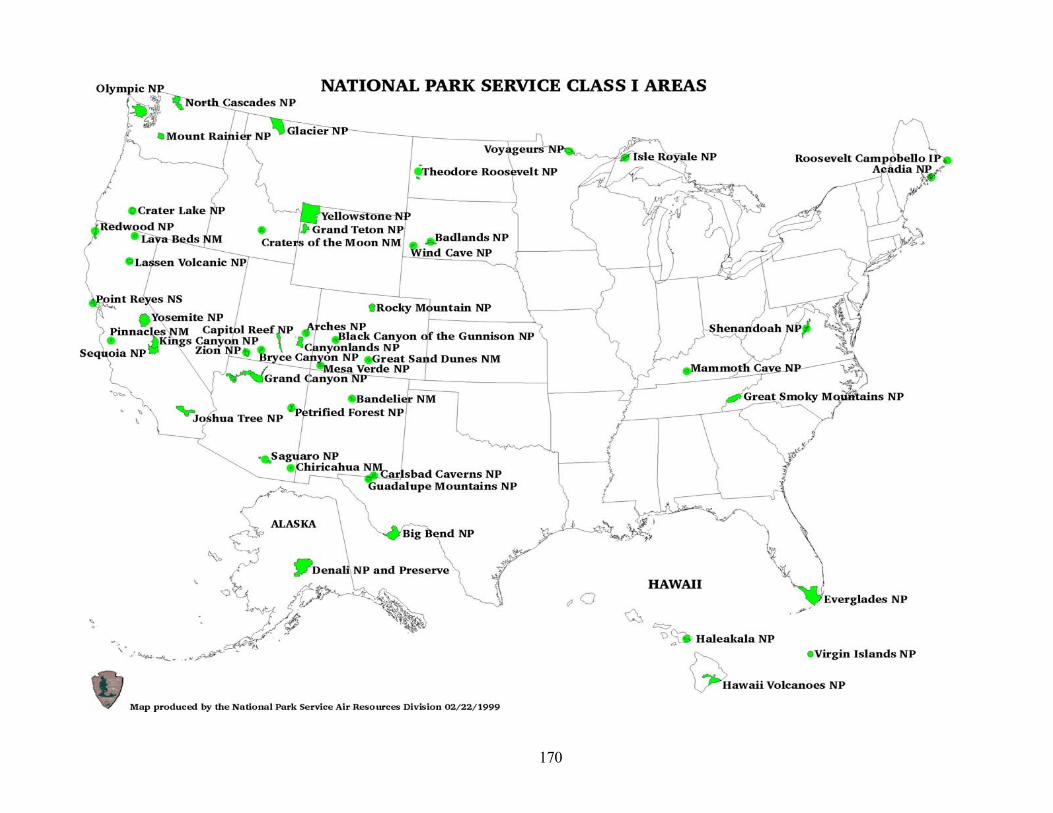
170

171

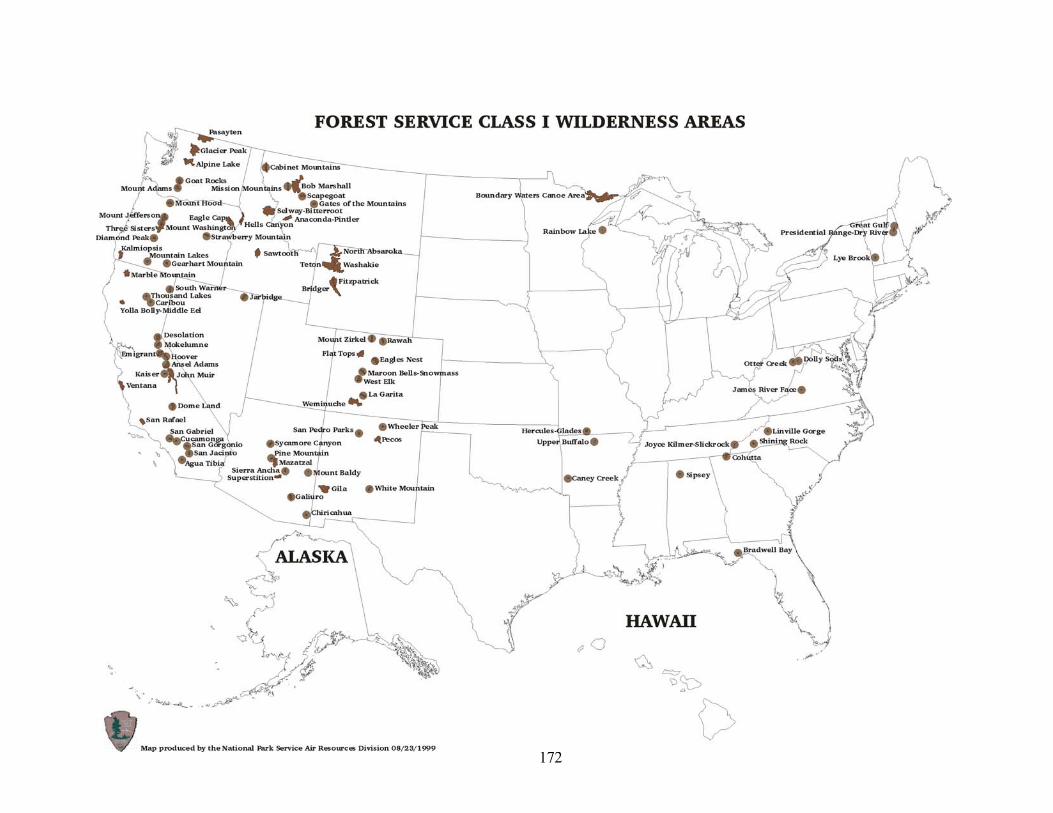
172

173

APPENDIX F. CLASS I AREA CONTACTS

USDA FOREST SERVICE CLASS I AREAS

REGION 1 Class I Areas: Anaconda-Pintler Wilderness Bob Marshall Wilderness Cabinet Mountains Wilderness Gates of the Mountains Wilderness Mission Mountains Wilderness Scapegoat Wilderness Selway-Bitterroot Wilderness Contact: Ann Acheson Phone Number: (406) 329-3493 Fax Number: (406) 329-3132 Email Address: [email protected] Mailing Address: USDA Forest Service, Region 1 P.O. Box 7669 Missoula, MT 59807

REGION 2

Class I Areas: Eagles Nest Wilderness Fitzpatrick Wilderness Flat Tops Wilderness La Garita Wilderness Maroon Bells - Snowmass Wilderness Mount Zirkel Wilderness North Absaroka Wilderness Rawah Wilderness Washakie Wilderness Weminuche Wilderness West Elk Wilderness Contact: Dennis Haddow Phone Number: (303) 275-5759 Fax Number: (303) 275-5754 Email Address: [email protected] Mailing Address: USDA Forest Service, Region 2 P.O. Box 25127 Lakewood, CO 80225-0127

174

REGION 3 Class I Areas: Chiricahua Wilderness Galiuro Wilderness Gila Wilderness Mazatzal Wilderness Mount Baldy Wilderness Pecos Wilderness Pine Mountain Wilderness San Pedro Parks Wilderness Sierra Ancha Wilderness Superstition Wilderness Sycamore Canyon Wilderness Wheeler Peak Wilderness White Mountain Wilderness Contact: Debby Potter, Ph.D. Phone Number: (505) 842-3143 Fax Number: (505) 842-3800 Email Address: [email protected] Mailing Address: USDA Forest Service, Southwestern Region Federal Building 517 Gold Ave., S.W. Albuquerque, NM 87102

REGION 4

Class I Areas: Bridger Wilderness Hells Canyon Wilderness* Hoover Wilderness Jarbidge Wilderness Sawtooth Wilderness* Teton Wilderness Contact: Dennis Haddow *Contact: Ann Acheson Phone Number: (303) 275-5759 Phone Number: (406) 329-3493 Fax Number: (303) 275-5754 Fax Number: (406) 329-3132 Email Address: [email protected] Email Address: [email protected] Mailing Address: Mailing Address: USDA Forest Service, Region 2 USDA Forest Service, Region 1 P.O. Box 25127 P.O. Box 7669 Lakewood, CO 80225-0127 Missoula, MT 59807

175

REGION 5 Class I Areas: Caribou Wilderness Marble Mountain Wilderness South Warner Wilderness Thousand Lakes Wilderness Yolla Bolly - Middle Eel Wilderness Contact: Suraj Ahuja Phone Number: (916) 934-5630 Fax Number: (916) 934-7384 Email Address: [email protected] Mailing Address: Mendocino National Forest 420 E. Laurel Street Willows, CA 95988 Class I Areas: Agua Tibia Wilderness Cucamonga Wilderness San Gabriel Wilderness San Gorgonio Wilderness San Jacinto Wilderness San Rafael Wilderness Ventana Wilderness Contact: Mike McCorison Phone Number: (818) 574-5286 Fax Number: (818) 574-5233 Email Address: [email protected]

Mailing Address: Angeles National Forest 701 N. Santa Anita Ave.

Arcadia, CA 91006

176

Class I Areas: Ansel Adams Wilderness Desolation Wilderness Dome Land Wilderness Emigrant Wilderness John Muir Wilderness Kaiser Wilderness Mokelumne Wilderness Contact: Trent Procter Phone Number: (559) 784 -1500, ext. 1114 Fax Number: (559) 781 - 4744 Email Address: [email protected] Mailing Address: Sequoia National Forest 900 W. Grand Ave. Porterville, CA 93257-2035

REGION 6

Class I Areas: Alpine Lakes Wilderness Diamond Peak Wilderness Eagle Cap Wilderness Gearhart Mountain Wilderness Glacier Peak Wilderness Goat Rocks Wilderness Hells Canyon Wilderness Kalmiopsis Wilderness Mt. Adams Wilderness Mt. Hood Wilderness Mt. Jefferson Wilderness Mt. Washington Wilderness Mountain Lakes Wilderness Pasayten Wilderness Strawberry Mountain Wilderness Three Sisters Wilderness Contact: Bob Bachman Phone Number: (503) 808 - 2918 Fax Number: (503) 808 - 2973 Email Address: [email protected] Mailing Address: USDA Forest Service, Region 6 P.O. Box 3623 Portland, OR 97208-3623

177

REGION 8 Class I Areas: Dolly Sods Wilderness James River Face Wilderness Otter Creek Wilderness Contact: Cindy Huber Phone Number: (540) 265-5156 Fax Number: (540) 265-5145 Email Address: [email protected] Mailing Address: Jefferson National Forest 5162 Valleypointe Parkway Roanoke, VA 24019 Class I Areas: Joyce Kilmer - Slickrock Wilderness Linville Gorge Wilderness Shining Rock Wilderness Contact: Bill Jackson Phone Number: (704) 257-4815 Fax Number: (704) 257-4263 Email Address: [email protected] Mailing Address: National Forests in North Carolina P.O. Box 2750 Asheville, NC 28802 Class I Areas: Caney Creek Wilderness Upper Buffalo Wilderness Contact: Laura Hudnell Phone Number: (501) 321-5235 Fax Number: (501) 321-5353 Email Address: [email protected] Mailing Address: Ouachita National Forest Box 1270, Federal Building Hot Springs Natl. Park, AR 71902

178

Class I Areas: Bradwell Bay Wilderness Cohutta Wilderness Sipsey Wilderness Contact: Dave Wergowske Phone Number: (334) 241-8137 Fax Number: (334) 241-8111 Email Address: [email protected] Mailing Address: National Forests in Alabama 2946 Chestnut Street Montgomery, AL 36107-3010

REGION 9

Class I Area: Boundary Waters Canoe Area Contact: Robert Berrisford Phone Number: (218) 720-5385 Fax Number: (218) 720-5600 Email Address: [email protected] Mailing Address: Superior National Forest Box 338, Federal Building 515 W. First St. Duluth, MN 55802 Class I Area: Lye Brook Wilderness Contact: Nancy Burt Phone Number: (802) 747-6742 Fax Number: (802) 747-6766 Email Address: [email protected] Mailing Address: Green Mountain National Forest 231 N. Main Street Rutland, VT 05701

179

Class I Areas: Great Gulf Wilderness Presidential Range - Dry River Wilderness Contact: Joan Carlson Phone Number: (603) 528-8721 Fax Number: (603) 528-8783 Email Address: [email protected] Mailing Address: White Mountain National Forest 719 Main Street Laconia, NH 03246-0772 Class I Area: Hercules - Glades Wilderness Contact: Laura Hudnell Phone Number: (501)321-5235 Fax Number: (501) 321-5353 Email Address: [email protected] Mailing Address: Mark Twain National Forest 401 Fairgrounds Road Rolla, MO 65401 Class I Area: Rainbow Lakes Wilderness Contact: Dale Higgins Phone Number: (715) 762-5181 Fax Number: (715) 762-5179 Email Address: [email protected] Mailing Address: Chequamegon National Forest 1170 4th Avenue South Park Falls, WI 54552

180

NATIONAL PARK SERVICE CLASS I AREAS

For inquiries regarding routine permit issues, contact the NPS Air Resources Division in Lakewood, Colorado: John Bunyak, Chief, Policy, Planning and Permit Review Branch; (303) 969-2818; [email protected]; P.O. Box 25287, Denver CO, 80225.

ALASKA REGION Denali National Park and Preserve Contact: Andrea Blakesley Phone Number: (907) 683-2294 Fax Number: (907) 683-9612 Email Address: [email protected] Mailing Address: P.O. Box 9 Denali Park, AK 99755

INTERMOUNTAIN REGION

Arches National Park Contact: Superintendent Phone Number: (801) 259-3911 Fax Number: (801) 259-8341 Mailing Address: P.O. Box 907 Moab, UT 84532 Bandelier National Monument Contact: Superintendent Phone Number: (505) 672-3861 Fax Number: (505) 672-9607 Mailing Address: HCR 1, Box 1, Suite 15 Los Alamos, NM 87544 Big Bend National Park Contact: Superintendent Phone Number: (915) 477-2251 Fax Number: (915) 477-2357 Mailing Address: P.O. Box 129 Big Bend National Park, TX 79834

181

Black Canyon of the Gunnison National Park Contact: Superintendent Phone Number: (970) 641-2337 Fax Number: (970) 641-2337 Mailing Address: P.O. Box 1648 Montrose, CO 81402 Bryce Canyon National Park Contact: Superintendent Phone Number: (435) 834-5322 Fax Number: (435) 834-4102 Mailing Address: P.O. Box 170001 Bryce Canyon, UT 84717 Canyonlands National Park Contact: Superintendent Phone Number: (801) 259-3911 Fax Number: (801) 259-8628 Mailing Address: P.O. Box 907 Moab, UT 84532 Capitol Reef National Park Contact: Superintendent Phone Number: (801) 425-3791 Fax Number: (801) 425-3026 Mailing Address: HC 70, Box 15 Torry, UT 84775 Carlsbad Caverns National Park Contact: Superintendent Phone Number: (505) 785-2232 Fax Number: (505) 785-2133 Mailing Address: 3225 National Parks Highway Carlsbad, NM 88220 Chiricahua National Monument Contact: Superintendent Phone Number: (520) 824-3560 Fax Number: (520) 824-3421 Mailing Address: Dos Cabezas Route, Box 6500 Willcox, AZ 85643

182

Glacier National Park Contact: Bill Michels Phone Number: (406) 888-5441 Fax Number: (406) 888-7901 Email Address: [email protected] Mailing Address: P.O. Box 128 West Glacier, MT 59936 Grand Canyon National Park Contact: Carl Bowman Phone Number: (520) 638-7817 Fax Number: (520) 638-7797 Email Address: [email protected] Mailing Address: P.O. Box 129 Grand Canyon, AZ 86023 Grand Teton National Park Contact: Superintendent Phone Number: (307) 739-3300 Fax Number: (307) 739-3438 Mailing Address: P.O. Box 170 Moose, WY 83012 Great Sand Dunes National Monument Contact: Superintendent Phone Number: (719) 378-2312 Fax Number: (719) 378-2594 Mailing Address: 11500 Highway 150 Mosca, CO 81146 Guadalupe Mountains National Park Contact: Superintendent Phone Number: (915) 828-3251 Fax Number: (915) 828-3269 Mailing Address: HC 60, Box 400 Salt Flat, TX 79847-9400

183

Mesa Verde National Park Contact: George San Miguel Phone Number: (970) 529-4465 Fax Number: (970) 529- 4498 Email Address: [email protected] Mailing Address: P.O. Box 8 Mesa Verde National Park, CO 81330 Petrified Forest National Park Contact: Superintendent Phone Number: (520) 524-6228 Fax Number: (520) 524-3567 Mailing Address: Box 2217 Petrified Forest National Park, AZ 86028 Rocky Mountain National Park Contact: Ken Czarnowski Phone Number: (970) 586-1263 Fax Number: (970) 586-1310 Email Address: [email protected] Mailing Address: Estes Park, CO 80517 Saguaro National Park Contact: Meg Weesner Phone Number: (520) 733-5170 Fax Number: (520) 733-5183 Email Address: [email protected] Mailing Address: 3693 South Old Spanish Trail Tucson, AZ 85730-5601 Yellowstone National Park Contact: Mary Hektner Phone Number: (307) 344-2151 Fax Number: (307) 344-2323 Email Address: [email protected] Mailing Address: P.O. Box 168 Yellowstone National Park, WY 82190

184

Zion National Park Contact: Jeff Bradybaugh Phone Number: (801) 772-0140 Fax Number: (801) 772-3426 Email Address: [email protected] Mailing Address: Springdale, UT 84767

MIDWEST REGION Badlands National Park Contact: Sandee Dingman Phone Number: (605) 433-5262 Fax Number: (605) 433-5404 Email Address: [email protected] Mailing Address: P.O. Box 6 Interior, SD 57750 Isle Royale National Park Contact: Superintendent Phone Number: (906) 482-0986 Fax Number: (906) 482-7170 Mailing Address: 87 North Ripley Street Houghton, MI 49931 Theodore Roosevelt National Park Contact: Russell Runge Phone Number: (701) 623-4466 Fax Number: (701) 623-4840 Email Address: [email protected] Mailing Address: P.O. Box 7 Medora, ND 58645 Voyageurs National Park Contact: Roger Andrascik Phone Number: (218) 283-9821 Fax Number: (218) 285-7407 Email Address: [email protected] Mailing Address: P.O. Box 50 International Falls, MN 56649

185

Wind Cave National Park Contact: Dan Roddy Phone Number: (605) 745-1157 Fax Number: (605) 745-4207 Email Address: [email protected] Mailing Address: RR 1, Box 190 Hot Springs, SD 57747

NORTHEAST REGION

Acadia National Park Contact: Bob Breen Phone Number: (207) 288-9561 Fax Number: (207) 288-5507 Email Address: [email protected] Mailing Address: P.O. Box 177 Bar Harbor, ME 04609 Shenandoah National Park Contact: Christi Gordon Phone Number: (540) 999-3499 Fax Number: (540) 999-3601 Email Address: [email protected] Mailing Address: 3655 U.S. Highway 211 East Luray, VA 22835

PACIFIC WEST REGION Crater Lake National Park Contact: Superintendent Phone Number: (541) 594-2211 Fax Number: (541) 584-2299 Mailing Address: P.O. Box 7 Crater Lake, OR 97604 Craters of the Moon National Monument Contact: Superintendent Phone Number: (208) 527-3257 Fax Number: (208) 527-3073 Mailing Address: P.O. Box 29 Arco, ID 83213

186

Haleakala National Park Contact: Superintendent Phone Number: (808) 572-9306 Fax Number: (808) 572-1304 Mailing Address: P.O. Box 369 Makawao, HI 96768 Hawaii Volcanoes National Park Contact: Superintendent Phone Number: (808) 985-6025 Fax Number: (808) 967-8186 Mailing Address: P.O. Box 52 Volcanoes, HI 96718 Joshua Tree National Park Contact: Chris Holbeck Phone Number: (760) 367-5501 Fax Number: (760) 367-6392 Email Address: [email protected] Mailing Address: 74485 National Monument Drive Twentynine Palms, CA 92277 Kings Canyon National Park Contact: Annie Esperanza Phone Number: (559) 565-3341 Fax Number: (559) 565-3730 Email Address: [email protected] Mailing Address: 47050 Generals Highway Three Rivers, CA 93271 Lassen Volcanic National Park Contact: Superintendent Phone Number: (530) 595-4444 Fax Number: (530) 595-3262 Mailing Address: P.O. Box 100 Mineral, CA 96063-0100

187

Lava Beds National Monument Contact: Chuck Barat Phone Number: (530) 667-2282 Fax Number: (530) 667-2737 Email Address: [email protected] Mailing Address: P.O. Box 867 Tulelake, CA 96134 Mount Rainier National Park Contact: Barbara Samora Phone Number: (360) 569-2177 x2301 Fax Number: (360) 569-2170 Email Address: [email protected] Mailing Address: Tahoma Woods, Star Route Ashford, WA 98304-9801 North Cascades National Park Contact: Leigh Smith Phone Number: (360) 856-5700 Fax Number: (360) 856-1934 Email Address: [email protected] Mailing Address: 2105 Highway 20 Sedro Woolley, WA 98284 Olympic National Park Contact: Cat Hoffman Phone Number: (360) 452-3011 Fax Number: (360) 452-0335 Email Address: [email protected] Mailing Address: 600 East Park Avenue Port Angeles, WA 98362 Pinnacles National Monument Contact: Chad Moore Phone Number: (408) 389-4485 Fax Number: (408) 389-4489 Email Address: [email protected] Mailing Address: 5000 Highway 146 Paicines, CA 95043

188

Point Reyes National Seashore Contact: Superintendent Phone Number: (415) 663-8522 Fax Number: (415) 663-8132 Mailing Address: Point Reyes Station Point Reyes, CA 94956 Redwood National Park Contact: Superintendent Phone Number: (707) 464-6101 Fax Number: (707) 464-1812 Mailing Address: 1111 Second Street Crescent City, CA 95531 Sequoia National Park Contact: Annie Esperanza Phone Number: (559) 565-3341 Fax Number: (559) 565-3730 Email Address: [email protected] Mailing Address: 47050 Generals Highway Three Rivers, CA 93271 Yosemite National Park Contact: Superintendent Phone Number: (209) 372-0265 Fax Number: (209) 372-0220 Mailing Address: P.O. Box 577 Yosemite National Park, CA 95389

SOUTHEAST REGION Everglades National Park Contact: Superintendent Phone Number: (305) 242-7710 Fax Number: (305) 242-7728 Mailing Address: P.O. Box 279 Homestead, FL 33030

189

Great Smoky Mountains National Park Contact: Jim Renfro Phone Number: (423) 436-1708 Fax Number: (423) 436-1220 Email Address: [email protected] Mailing Address: 107 Park Headquarters Road Gatlinburg, TN 37738 Mammoth Cave National Park Contact: Bobby Carson Phone Number: (502) 749-2508 Fax Number: (520) 749-2349 Email Address: [email protected] Mailing Address: P.O. Box 7 Mammoth Cave, KY 42259 Virgin Islands National Park Contact: Superintendent Phone Number: (809) 775-6238 Fax Number: (809) 775-7025 Mailing Address: 6310 Estate Nazareth #10 St. Thomas, VI 00802

190

U.S. FISH AND WILDLIFE SERVICE CLASS I AREAS

For inquiries regarding routine permit issues, contact the FWS Air Quality Branch in Lakewood, Colorado: Sandra Silva, Chief; (303) 969-2814; [email protected]; P.O. Box 25287, Denver CO, 80225.

REGION 2 Bosque Del Apache Wilderness Contact: Refuge Manager Phone Number: (505) 835-1828 Fax Number: (505) 835-0314 Mailing Address: Bosque del Apache NWR P.O. Box 1246 Socorro, NM 87801 Salt Creek Wilderness Contact: Refuge Manager Phone Number: (505) 662-6755 Fax Number: (505) 623-9039 Mailing Address: Bitter Lake NWR P.O. Box 7 Roswell, NM 88202-0007 Wichita Mountains Wilderness Contact: Refuge Manager Phone Number: (580) 429-3007 Fax Number: (580) 429-9323 Email Address: [email protected] Mailing Address: Wichita Mountains NWR Rt. 1, Box 448 Indiahoma, OK 73552

REGION 3 Seney Wilderness Contact: Refuge Manager Phone Number: (906) 586-9851 Fax Number: (906)586-3800 Email Address: [email protected] Mailing Address: Seney NWR HCR 2, Box 1 Seney, MI 49883

191

Mingo Wilderness Contact: Refuge Manager Phone Number: (573) 222-3589 Fax Number: (573) 222-6343 Email Address: [email protected] Mailing Address: Mingo NWR Route 1, Box 103 Puxico, MO 63960

REGION 4 Breton Wilderness Contact: Refuge Manager Phone Number: (504) 646-7555 Fax Number: (504) 646-7588 Email Address: [email protected] Mailing Address: Bogue Chitto NWR 1010 Gause Blvd., Bldg. 936 Slidell, LA 70458 Cape Romain Wilderness Contact: Refuge Manager Phone Number: (803) 928-3264 Fax Number: (803) 928-3803 Email Address: [email protected] Mailing Address: Cape Romain NWR 5801 Highway 17 North Awendaw, SC 29429 Chassahowitzka Wilderness Contact: Refuge Manager Phone Number: (352) 563-2088 Fax Number: (352) 795-7961 Mailing Address: Chassahowitzka NWR 1502 S. Kings Bay Drive Crystal River, FL 32629

192

Okefenokee Wilderness Contact: Refuge Manager Phone Number: (912) 496-7366 Fax Number: (912) 496-7366 Mailing Address: Okefenokee NWR Route 2, Box 3330 Folkston, GA 31537 St. Marks Wilderness Contact: Refuge Manager Phone Number: (850) 925-6121 Fax Number: (850) 925-6930 Email Address: [email protected] Mailing Address: St. Marks NWR P.O. Box 68 St. Marks, FL 32355 Swanquarter Wilderness Contact: Refuge Manager Phone Number: (252) 926-4021 Fax Number: (252) 926-1743 Email Address: [email protected] Mailing Address: Mattamuskeet NWR Route 1, Box N-2 Swanquarter, NC 27885 Wolf Island Wilderness Contact: Refuge Manager Phone Number: (912) 652-4415 Fax Number: (912) 652-4385 Mailing Address: Savannah Coastal Refuges 1000 Business Center Dr., Ste. 10 Savannah, GA 31405

REGION 5 Brigantine Wilderness Contact: Refuge Manager Phone Number: (609) 652-1665 Fax Number: (609) 652-1474 Email Address: R5RW_FBRNWR @fws.gov Mailing Address: Edwin B. Forsythe NWR P.O. Box 72, Great Creek Rd. Oceanville , NJ 08231

193

Moosehorn Wilderness Contact: Refuge Manager Phone Number: (207) 454-3521 Fax Number: (207) 454-2550 Email Address: [email protected] Mailing Address: Moosehorn NWR R.R. 1 Box 202, Suite 1 Baring, ME 04694-9703

REGION 6 Lostwood Wilderness Contact: Refuge Manager Phone Number: (701) 848-2722 Fax Number: (701) 848-2702 Mailing Address: Lostwood NWR R.R. 2 Box 98 Kenmare, ND 58746-9046 Medicine Lake Wilderness Contact: Refuge Manager Phone Number: (406) 789-2305 Fax Number: (406) 789-2350 Mailing Address: Medicine Lake NWR 223 North Shore Road Medicine Lake, MT 59247 Red Rock Lakes Wilderness Contact: Refuge Manager Phone Number: (406) 276-3536 Fax Number: (406) 276-3538 Mailing Address: Red Rock Lakes NWR Monida Star Route, Box 15 Lima, MT 59739 UL Bend Wilderness Contact: Refuge Manager Phone Number: (406) 538-8706 Fax Number: (406) 538-7521 Mailing Address: Charles M. Russell NWR P.O. Box 110 Lewistown, MT 59457

194

REGION 7 Bering Sea/Simeonof/Tuxedni Wilderness Areas Contact: Refuge Manager Phone Number: (907) 235-6546 Fax Number: (907) 235-7783 Mailing Address: Alaska Maritime NWR 2355 Kachemak Bay Drive, Suite 101 Homer, AK 99603

195

APPENDIX G. FLAG PARTICIPANTS

The individuals listed in the attached table participated in the development of the FLAG Phase I Report. The abbreviations for the FLAG subgroup or committee on which participants served are shown below. LC = Leadership Committee CC = Coordinating Committee P = Policy Subgroup V = Visibility Subgroup O = Ozone Subgroup D = Deposition Subgroup T = Terminology (Glossary) Subgroup

196

FLAG PARTICIPANTS

Name Subgroup Organization Work Phone Fax Email Address

Acheson, Ann V Forest Service (406) 329-3493 (406) 329-3132 [email protected]

Ahuja, Suraj O,V,D Forest Service (530) 934-3316 (530) 934-7384 [email protected]

Bachman, Bob CC,V,D,T Forest Service (503) 808-2918 (503) 808-2973 [email protected]

Bayle, Bruce P Forest Service (404) 347-3872 (404) 347-6197 [email protected]

∗Benoit, Clif V,P Forest Service -- -- --

Blanchard, Karen EPA (919) 541-5503 (919) 541-5509 [email protected]

∗Blett, Tamara Forest Service -- -- --

Boutcher, Steve Forest Service (503) 326-5434 (503) 808-2973 [email protected]

Bray, David T,V EPA (206) 553-4253 (206) 553-0110 [email protected]

∗Breitenfeld, Dale Park Service -- -- --

Bunyak, John P,T Park Service (303) 969-2818 (303) 969-2822 [email protected]

Bytnerowicz, A. O Forest Service (909) 680-1562 (909) 680-1501 [email protected]

∗Carriero, Joe CC,T Fish and Wildlife -- -- --

Copeland, Scott V CIRA (CSU) (970) 491-3315 (970) 491-8598 [email protected]

Fisher, Rich CC,V,P,O,T Forest Service (970) 498-1232 (970) 498-1010 [email protected]

∗Flores, Miguel P,O Park Service -- -- --

∗ No longer works for the agency, or now works for a different office.

197


Haddow, Dennis P,V,T Forest Service (303) 275-5759 (303) 275-5754 [email protected]

Hogsett, Bill O EPA (541) 754-4632 (541) 754-4739 [email protected]

Huber, Cindy V Forest Service (540) 265-5156 (540) 265-5145 [email protected]

Irwin, John V EPA (919) 541-5682 (919) 541-0044 [email protected]

Jackson, Bill O Forest Service (704) 257-4815 (704) 257-4263 [email protected]

Lamb, Donna LC Forest Service (202) 205-0800 (202) 205-1096 [email protected]

Malm, Bill V Park Service (970) 491-8292 (970) 491-8598 [email protected]

Maniero, Tonnie CC,O Park Service (303) 969-2806 (303) 969-2822 [email protected]

Morris, Kristi Park Service (303) 987-6941 (303) 969-2822 [email protected]

Morse, Dee CC,V Park Service (303) 969-2817 (303) 969-2822 [email protected]

Musselman, Bob O,D Forest Service (970) 498-1239 (970) 498-1010 [email protected]

Notar, John V Park Service (303) 969-2079 (303) 969-2822 [email protected]

∗Parker, Kim D,O Forest Service -- -- --

Peterson, Dave O BRD (206) 543-1587 (206) 695-0790 [email protected]

Peterson, Janice O,D Forest Service (425) 744-3425 (425) 744-3255 [email protected]

Pitchford, Mark V NOAA (702) 895-0432 (702) 895-0507 [email protected]

Pitt, Ken P USDA/OGC (303) 275-5539 (303) 275-5557 [email protected]

Porter, Ellen CC,D Fish and Wildlife (303) 969-2617 (303) 969-2822 [email protected]

Potter, Debby P,D Forest Service (505) 842-3143 (505) 842-3800 [email protected]

Procter, Trent O Forest Service (559) 784-1500 (559) 781-4744 [email protected]

∗ No longer works for the agency or now works for a different office.

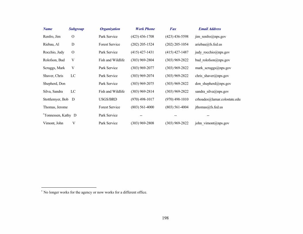
198


Renfro, Jim O Park Service (423) 436-1708 (423) 436-5598 [email protected]

Riebau, Al D Forest Service (202) 205-1524 (202) 205-1054 [email protected]

Rocchio, Judy O Park Service (415) 427-1431 (415) 427-1487 [email protected]

Rolofson, Bud V Fish and Wildlife (303) 969-2804 (303) 969-2822 [email protected]

Scruggs, Mark V Park Service (303) 969-2077 (303) 969-2822 [email protected]

Shaver, Chris LC Park Service (303) 969-2074 (303) 969-2822 [email protected]

Shepherd, Don Park Service (303) 969-2075 (303) 969-2822 [email protected]

Silva, Sandra LC Fish and Wildlife (303) 969-2814 (303) 969-2822 [email protected]

Stottlemyer, Bob D USGS/BRD (970) 498-1017 (970) 498-1010 [email protected]

Thomas, Jerome Forest Service (803) 561-4000 (803) 561-4004 [email protected]

∗Tonnessen, Kathy D Park Service -- -- --

Vimont, John V Park Service (303) 969-2808 (303) 969-2822 [email protected]

∗ No longer works for the agency or now works for a different office.

199

APPENDIX H. BIBLIOGRAPHY

Some of the documents cited below were referenced in this FLAG Phase I Report. Others are listed to provide background information.

General References Adams, M.B., D.S. Nichols, C.A. Federer, K.F. Jensen and H. Parrott. 1991. Screening Procedure to Evaluate Effects of Air Pollution on Eastern Region Wildernesses Cited as Class I Air Quality Areas. General Technical Report NE-151. U.S. Department of Agriculture, Forest Service, Northeastern Forest Experiment Station. Radnor, Pennsylvania. Binkley, D., C. Giardina, I. Dockersmith, D. Morse, M. Scruggs and K. Tonnessen. 1997. Status of Air Quality and Related Values in Class I National Parks and Monuments of the Colorado Plateau. U.S. Department of the Interior, National Park Service, Air Resources Division. Denver, Colorado. Blankenship, J.O., D.U. Potter, R.W. Fisher and J.M. Eilers. In Press. Guidelines for Evaluating Air Pollution Impacts on Class I Areas in the Southwestern Region. U.S. Department of Agriculture, Forest Service, Rocky Mountain Research Station. Ft. Collins, Colorado. Bunyak, J. 1993. Permit Application Guidance for New Pollution Sources. Natural Resources Report NPS/NRAQD/NRR-93. U.S. Department of the Interior, National Park Service, Air Quality Division. Denver, Colorado. Eilers, J. M., C.L. Rose and T.J. Sullivan. 1994. Status of Air Quality and Effects of Atmospheric Pollutants on Ecosystems in the Pacific Northwest Region of the National Park Service. Technical Report NPS/NRAQD/NRTR-94/160. U.S. Department of the Interior, National Park Service, Air Quality Division. Denver, Colorado. Fox, D.G., A.M. Bartuska, J.G. Byrne, E. Cowling, R. Fisher, G.E. Likens, S.E. Lindberg, R.A. Linthurst, J. Messer and D.S. Nichols. 1989. A Screening Procedure to Evaluate Air Pollution Effects on Class I Wilderness Areas. General Technical Report RM-168. U.S. Department of Agriculture, Forest Service, Rocky Mountain Forest and Range Experiment Station. Ft. Collins, Colorado. Fox, D., G.J.C. Bernabo and B. Hood. 1987. Guidelines for Measuring the Physical, Chemical, and Biological Condition of Wilderness Ecosystems. General Technical Report RM-146. U.S. Department of Agriculture, Forest Service, Rocky Mountain Forest and Range Experiment Station. Ft. Collins, Colorado. Garner, J.H.B., T. Pagano and E.B. Cowling. 1989. An Evaluation of the Role of Ozone, Acid Deposition, and Other Airborne Pollutants in the Forests of Eastern North America. General Technical Report SE-59. U.S. Department of Agriculture, Forest Service, Southeastern Forest Experiment Station. Asheville, North Carolina.

200

Haddow, D., R. Musselman, T. Blett and R. Fisher. 1998. Guidelines for Evaluating Air Pollution Impacts on Wilderness within the Rocky Mountain Region: Report of a Workshop, 1990. General Technical Report RMRS-GTR-4. U.S. Department of Agriculture, Forest Service, Rocky Mountain Research Station. Ft. Collins, Colorado. Ottmar, R. 1996. Linking recent historical and current forest vegetation patterns to smoke and crown fire in the Interior Columbia River Basin. Paper presented at the 13th Conference of Fire and Forest Meteorology, October 27-31, 1996. Lorne, Australia. Peterson, D.L., D.L. Schmoldt, J.M. Eilers, R.W. Fisher and R.D. Doty. 1993. Guidelines for Evaluating Air Pollution Impacts on Class I Wilderness Areas in California. General Technical Report PSW-GTR-136. U.S. Department of Agriculture, Forest Service, Pacific Southwest Research Station. Albany, California. Peterson, D.L., T.J. Sullivan, J.M. Eilers, S. Brace, D. Horner and K. Savig. 1998. Assessment of Air Quality and Air Pollutant Impacts in National Parks of the Rocky Mountains and Northern Great Plains. U.S. Department of the Interior, National Park Service, Air Resources Division. Peterson, J., D. Schmoldt, D. Peterson, J. Eilers, R. Fisher and R. Bachman. 1992. Guidelines for Evaluating Air Pollution Impacts on Class I Wilderness Areas in the Pacific Northwest. General Technical Report PNW-GTR-299. U.S. Department of Agriculture, Forest Service, Pacific Northwest Research Station. Portland, Oregon. Porter, E. 1996. Air Quality and Air Quality Related Values in Chassahowitzka National Wildlife Refuge and Wilderness Area. U.S. Fish and Wildlife Service, Air Quality Branch. Denver, Colorado. Stanford, J., A. Acheson, D. Brakke, S. Eversman, K. Savig and J. Eilers. 1997. A Screening Procedure to Evaluate Air Pollution Effects in Region 1 Wilderness Areas, 1991. General Technical Report RM-GTR-294. U.S. Department of Agriculture, Forest Service, Rocky Mountain Forest and Range Experiment Station. Ft. Collins, Colorado. Turner, R. S., D. G. Fox, A. Bartuska, W. Jackson and B. Bayle. Draft. Screening Procedures to Evaluate Effects of Air Pollution on Forest Service Wilderness in the Southern Region. USDA Forest Service. 2000. Screening Methodology for Calculating ANC Change to High Elevation Lakes. Rocky Mountain Region. January 2000. U.S. EPA. 1998. Interim Air Quality Policy on Wildland and Prescribed Fires. Office of Air Quality Planning and Standards. Research Triangle Park, North Carolina. 39 pp.

201

Visibility References Colorado State University. Cooperative Institute for Research in the Atmosphere. 1996 IMPROVE, Interagency Monitoring of Protected Environments. Spatial and Seasonal Patterns and Long Term Variability of the Composition of the Haze in the United States: An Analysis of Data from the IMPROVE Network. National Acid Precipitation Assessment Program. 1990. Acidic Deposition: State of Science and Technology, Report 24, Visibility: Existing and Historical Conditions – Causes and Effects. National Park Service. 1993. Permit Application Guidance for New Pollution Sources. Natural Resources Report NPS/Nraqd/NRR-93. Pitchford, M.L. and Malm, W.C. 1994. Development and Applications of a Standard Visual Index. Atmospheric Environment 28, 1049-1054. USEPA. 1992a. Workbook for Visual Impact Screening and Analysis (Revised). EPA-450/R-92-023 USEPA. 1992b. User’s Manual for the Plume Visibility Model, PLUVUE II (Revised). EPA-454/B-92-008. USEPA. 1996a. CALMET, CALPUFF, and CALPOST Modeling System. PB 96-502-083INC. USEPA. 1996b. Proposed Rule, New Source Review Reform, Federal Register/Vol. 61, No. 142/Tuesday, July 23, 1996. USEPA. 1996c. Addendum to the User’s Manual for the Plume Visibility Model, PLUVUE II (Revised). EPA-454/B-95-001. USEPA. 1998. Interagency Workgroup on Air Quality Modeling (IWAQM) Phase 2 Summary Report and Recommendations for Modeling Long-Range Transport and Impacts on Regional Visibility. EPA-454/R-98-019.

202

Ozone References Ashmore, M.R. and A.W. Davison. 1996. Towards a critical level of ozone for natural vegetation. In: Kaerenlampi, L. and L. Skaerby, eds. Critical Levels for Ozone in Europe: Testing and Finalizing the Concepts. UN-ECE Workshop Report. University of Kuopio, Department of Ecology and Environmental Science. p. 58-71. Brace, S., D.L. Peterson and D. Horner. 1998. Diagnosing Ozone Injury in Vascular Plants of the Pacific Northwest. PNW-GTR-xxx (In Press). U.S. Department of Agriculture, Forest Service, Pacific Northwest Research Station. Chappelka, A.H., L.J. Samuelson, J.M. Skelly, A.S. Lefohn and D. Nesdill. 1995. Effects of Ozone on Vegetation in Southern Appalachians: an Annotated Bibliography. Auburn University, School of Forestry. Auburn, Alabama. Davis, D.D. 1995. Evaluation of Ambient Ozone Injury on the Foliage of Vegetation in the Edwin B. Forsythe National Wildlife Refuge, Brigantine, New Jersey. Final Report. Davis, D.D. 1998. Evaluation of Ambient Ozone Injury on the Foliage of Vegetation in the Cape Romain National Wildlife Refuge, South Carolina. 1997 Observations. Davis, D.D. 1998. Evaluation of Ozone Injury on Vegetation in the Okefenokee National Wildlife Refuge, Georgia. 1997 Observations. Eckert, R., R. Kohut, J. Laurence, P. King, T. Lee, B. Rock, D. Moss and A. Theisen. 1991. Studies to Assess the Effects of Ozone on Native Vegetation of Acadia National Park. Annual Report. University of New Hampshire. Durham, New Hampshire. Guderian, R., D.T. Tingey, and R. Rabe. 1985. Effects of photochemical oxidants on plants. Part 2. In: Guderian, R., ed. Air Pollution by Photochemical Oxidants. Springer-Verlag. New York. p. 129-296. Guderian, R. 1977. Air Pollution. Phytotoxicity of Acidic Gases and Its Significance in Air Pollution Control. Springer-Verlag. New York. Heck, W.W. and E.B. Cowling. 1997. The need for a long-term cumulative secondary ozone standard - an ecological perspective. Environmental Management. January. Heck, W.W., C.S. Furiness, C.K. Simms and E.B. Cowling, eds. 1997. Report from Workshop on Research Needs to Assess the Effects of Ozone on Crop, Forest and Natural Ecosystems. May 18, 1997. Southern Oxidants Study, North Carolina State University. Raleigh, North Carolina. Kaerenlampi, L. and L. Skaerby, eds. 1996. Critical Levels for Ozone in Europe: Testing and Finalizing the Concepts. UN-ECE Workshop Report. University of Kuopio, Department of Ecology and Environmental Science.

203

Lefohn, A.S. 1998. The Identification of Ozone Exposures that Result in Vegetation Visible Injury and Growth Loss for Specific Species Grown in the Southern Appalachian Mountain Region. Southern Appalachian Mountains Initiative Report. Lefohn, A.S. and V.C. Runeckles. 1987. Establishing a standard to protect vegetation - ozone exposure/dose considerations. Atmospheric Environment 21(3):561-568.

Massman, W.J., R.C. Musselman, and A.S. Lefohn. 2000. A conceptual ozone dose-response model to develop a standard to protect vegetation. Atmospheric Environment 34:745-759.

Miller, P., R. Guthrey and S. Schilling. 1995 Draft. Third Progress Report of FOREST. Comparisons of 1991-1995 Ozone Injury Index at Sierra Nevada and San Bernardino Mountains Sites. 9 pp. Miller, P.R., K.W. Stolte, D.M. Duriscoe and J. Pronos. 1996. Evaluating Ozone Air Pollution Effects on Pines in the Western United States. General Technical Report PSW-GTR-155. U.S. Department of Agriculture, Forest Service, Pacific Southwest Research Station. Albany, California. Miller, P., R. Guthrey, S. Schilling and J. Carroll. 1996. Ozone injury responses of ponderosa and Jeffrey pine in the Sierra Nevada and San Bernardino Mountains in California. Paper presented at International Symposium: Air Pollution and Climate Change Effects on Forest Ecosystems, Feb 5-9, 1996. U.S. Department of Agriculture, Forest Service, Pacific Southwest Research Station. Riverside, California. Multi-stakeholder NOx/VOC Science Program. 1997. Report of the Vegetation Objective Working Group: Canadian 1996 NOx/VOC Science Assessment. Atmospheric Environment Service, Environment Canada. Toronto, Ontario, Canada. Musselman, R.C. and T.J. Minnick. 2000. Nocturnal stomatal conductance and ambient air quality standards for ozone. Atmospheric Environment 34:719-733. Neufeld, H.S. and J.R. Renfro. 1993a. Sensitivity of Black Cherry Seedlings (Prunus serotina Ehrh.) to Ozone in Great Smoky Mountains National Park. The 1989 Seedling Set. Natural Resources Report NPS/NRTR-93/112. U.S. Department of the Interior, National Park Service, Air Quality Division. Denver, Colorado. 26 pp. Neufeld, H.S. and J.R. Renfro. 1993b. Sensitivity of Sycamore Seedlings (Platanus occidentalis) to Ozone in Great Smoky Mountains National Park. Data from 1989. Natural Resources Report NPS/NRTR-93/131. U.S. Department of the Interior, National Park Service, Air Quality Division. 39 pp. Singh, H.B.; Ludwig, F.L.; Johnson, W.B. 1978. Tropospheric ozone: concentrations and variabilities in clean remote atmospheres. Atmospheric Environment 12:2185-2196. Singh, H.B.; Viezee, W.; Johnson, W.B.; Ludwig, F.L. 1980. The impact of stratospheric ozone on trpospheric air quality. Journal Air Pollution Control Association 30:1009-1017.

204

Skaerby, L. and P.E. Karlsson. 1996. Critical levels for ozone to protect forest trees - best available knowledge from the nordic countries and the rest of Europe. In: Kaerenlampi, L. and L. Skaerby, eds. Critical Levels for Ozone in Europe: Testing and Finalizing the Concepts. UN-ECE Workshop Report. University of Kuopio, Department of Ecology and Environmental Science. p. 72-85. U.S. EPA. 1992. Summary of Selected New Information on Effects of Ozone on Health and Vegetation: Supplement to 1986 Air Quality Criteria for Ozone and Other Photochemical Oxidants. EPA/600/8-88/105F. Research Triangle Park, NC: US Environmental Protection Agency, Office of Health and Environmental Assessment. U.S. EPA. 1996a. Review of National Ambient Air Quality Standards for Ozone Assessment of Scientific and Technical Information. OAQPS Staff Paper. EPA-452/R-96-007. U.S. EPA, Office of Air Quality Planning and Standards. Research Triangle Park, North Carolina. U.S. EPA. 1996b. Air Quality Criteria for Ozone and Related Photochemical Oxidants. Vol. 2. EPA/600/P-93/004bF. U.S. EPA, Office of Research and Development. Research Triangle Park, North Carolina. Wooldridge, G; Zeller, K.; Musselman, R. 1997. Ozone concentration characteristics at a high-elevation forest site. Theoretical and Applied Climatology 56:153-164.

205

Deposition References

Aber, J.D., K.J. Nadelhoffer, P. Steudler and J.M. Melillo. 1989. Nitrogen saturation in northern forest ecosystems: excess nitrogen from fossil fuel combustion may stress the biosphere. BioScience 39:378-386. Adams, M.B., T.R. Angradi and J.N. Kochenderfer. 1997. Stream water and soil solution responses to 5 years of nitrogen and sulfur additions at the Fernow Experimental Forest, West Virginia. Forest Ecology and Management 95:79-91. Anderson, J.B., R.E. Baumgardner, V.A. Mohnen and J.J. Bowser. 1999. Cloud chemistry in the eastern United States, as sampled from three high-elevation sites along the Appalachian Mountains. Atmospheric Environment 33:5105-5114. Au, S. 1974. Vegetation and Ecological Processes on Shackleford Bank, North Carolina. Scientific Monograph Series No. 6. U.S. Department of the Interior, National Park Service. Washington, D.C. 86 pp. Baldocchi, D. D., B. B. Hicks and P. Camara 1987. A canopy stomatal resistance model for gaseous deposition to vegetated surfaces. Atmospheric Environment, 21, 91-101. Baron, J.S. and D.H. Campbell. 1997. Nitrogen fluxes in a high elevation Colorado Rocky Mountain basin. Hydrological Processes 11:783-799. Bormann, F. H. and G. E. Likens. 1967. Nutrient cycling. Science 155:424-429. Byron, E. R. and P. Eloranta. 1984. Recent historical changes in the diatom community of Lake Tahoe, California-Nevada, U.S.A. Verh. Internat. Verin. Limnol. 22:1372-1376. Bytnerowicz, A., J. J. Carroll, B. K. Takemoto, P. R. Miller, M. E. Fenn, R. C. Musselman. 2000. Distribution and transport of air pollutants to vulnerable California ecosystems. In: K. M. Scow, G. E. Fogg, M. L. Johnson. Integrated Assessment of Ecosystem Health, Lewis Publishers, Boca Raton, 93-118. Bytnerowicz, A., M. E. Fenn 1996. Nitrogen deposition in California forests: a review. Environmental Pollution, 92, 127-146. Bytnerowicz, A., M. E. Fenn, P. R. Miller, M. J. Arbaugh. 1999. Wet and dry pollutant deposition to the mixed conifer forest. In: P. R. Miller and J. R. McBride (eds.) Oxidant Air Pollution Impacts in the Montane Forests of Southern California. Springer, New York, 235-269. Bytnerowicz, A., S. Ferguson, F. Fujioka, R. Ottmar, M. Poth. 1997. Simulation modeling: role and status. In: A. Bytnerowicz (tech. ed.) Atmpospheric and Biospheric Interactions of Gases and Energy in the Pacific Region of the United States, Mexico and Brazil. USDA FS, Pacific Southwest Research Station, General Technical Report, PSW-GTR-161, 27-30.

206

California Air Resources Board (CARB). 1993. The Atmospheric Acidity Protection Program: Annual Report to the Governor and Legislature, 1992. Sacramento, California. Campbell, D.H., D.W. Clow, G.P. Ingersoll, M.A. Mast, N.E. Spahr and J.T. Turk. 1995. Processes controlling the chemistry of two snowmelt-dominated streams in the Rocky Mountains. Water Resources Research 31(11):2811-2821. CENR. 1999. The role of monitoring networks in the management of the Nation’s air quality. Report of the National Science and Technology Council Committee on Environment and Natural Resources. Washington, D.C. March 1999. Cosby, B.J., S.A. Norton and J.S. Kahl. 1996. Using a paired-watershed manipulation experiment to evaluate a catchment-scale biogeochemical model. Science of the Total Environment 183:49-66. Cosby, B.J., R.F. Wright and E. Gjessing. 1995. An acidification model (MAGIC) with organic acid evaluated using whole-catchment manipulations in Norway. J. Hydrol. 170:101-122. Cosby, B.J., R.F. Wright, G.M. Hornberger and J.N. Galloway. 1985. Modeling the effects of acid deposition: assessment of a lumped parameter model of soil water and streamwater chemistry. Water Resources Research 21:51-63. Dise, N. and R.F. Wright. 1995. Nitrogen leaching from European forests in relation to nitrogen deposition. Forest Ecology and Management 71:153-161. Dixon, L.K. and E.D. Estevez. 2000. Reservoirs of nitrogen and phosphorus across a multiple source, nitrogen-enriched, estuarine gradient. Draft report to the Air Quality Branch, U.S. Fish and Wildlife Service, Denver, Colorado. Ecological Society of America. 2000. Acid deposition: the ecological response. Workshop Report. March 1-3, 1999. Washington, D.C. Fenn, M.E. 1991. Increased site fertility and litter decomposition rate in high-pollution sites in the San Bernardino Mountains. For. Sci. 37(4):1163-1181. Fenn, M.E. and P.H. Dunn. 1989. Litter decomposition across an air-pollution gradient in the San Bernardino Mountains. Soil Sci. Soc. Am. J. 53(5):1560-1566. Fenn, M.E., M.A. Poth and D.W. Johnson. 1996. Evidence for nitrogen saturation in the San Bernardino Mountains in southern California. Forest Ecology and Management 82:211-230. Hanson, P. J., S. E. Lindberg. 1991. Dry deposition of reactive nitrogen compounds: a review of leaf, canopy and non-foliar measurements. Atmospheric Environment, 25A, 1615-1634.

207

Hedin, L.O. and G.E. Likens. 1996. Atmospheric dust and acid rain. Scientific American 275(6):88-92. Hemmerlein, M.T. and T.D. Perkins. 1993. Techniques for pollution monitoring in remote sites: III. near real-time monitoring of cloud water conductivity and pH. Water, Air, and Soil Pollution 71(1/2). Herlihy, A.T., P.R. Kaufmann, J.L. Stoddard, K.N. Eshleman and A.J. Bulger. 1996. Effects of Acidic Deposition on Aquatic Resources in the Southern Appalachians with a Special Focus on Class I Wilderness Areas. Submitted to the Southern Appalachian Mountains Initiative. 91 pp. Hicks, B. B., D. D. Baldocchi, T. P. Meyers, R. P. Hosker, D. R. Matt. 1987. A preliminary multiple resistance routine for deriving dry deposition velocities from measured quantities. Water, Air and Soil Pollution, 36:311-330. Hidy, G.M. 1998. Dry deposition relevant to the National Parks and Wildernesses. Report to the Cooperative Institute for Research in the Atmosphere. Fort Collins, Colorado. Holm-Hansen, O., C.R. Goldman, R. Richards and P.M. Williams. 1976. Chemical and biological characteristics of a water column in Lake Tahoe. Limnol. Oceanogr. 21(4):548-562. Jackson, L., L. Geiser, T. Blett, C. Gries and D. Haddow. 1996. Biogeochemistry of Lichens and Mosses in and Near Mt. Zirkel Wilderness, Routt National Forest, Colorado: Influences of Coal-Fired Power Plant Emissions. Open File Report 96-295. U.S. Department of the Interior, U.S. Geological Survey. Jassby, A.D., C.R. Goldman and J.E. Reuter. 1995. Long-term change in Lake Tahoe (California-Nevada, U.S.A.) and its relation to atmospheric deposition of algal nutrients. Arch. Hydrobiol. 135(1):1-21. Johnson, D.W. and G.S. Henderson. 1979. Sulfate adsorption and sulfur fractions in a highly weathered soil under a mixed deciduous forest. Soil Sci. 128(1):34-40. Johnson, D.W., H. Van Miegroet, D. Cole and D. Richter. 1983. Contributions of acid deposition and natural processes to cation leaching from forest soils: a review. J. Air Pollut. Control Assoc. 33:1036-1041. Junge, C.E. 1958. The distribution of ammonia and nitrate in rain water over the United States. Trans. Amer. Geophys. Union 39(2):241-248. Kendall, C., D.H. Campbell, D.A. Burns, J.B. Shanley, S.R. Silva and C.C.Y. Chang. 1995. Tracing sources of nitrate in snowmelt runoff using the oxygen and nitrogen isotopic compositions of nitrate. In: Tonnessen, K.A. and M.W. Williams (eds), Biogeochemistry of Seasonally-Covered Catchments. IAHS Publ. No. 228. p. 339-347.

208

Langford, A.O., F.C. Fehsenfeld, J. Zachariassen and D.S. Schimel. 1992. Gaseous ammonia fluxes and background concentrations in terrestrial ecosystems of the United States. Global Biogeochemical Cycles 6(4):459-483. Leonard, R.L., L.A. Kaplan, J.F. Elder, R.N. Coats and C.R. Goldman. 1979. Nutrient transport in surface runoff from a subalpine watershed, Lake Tahoe Basin, California. Ecol. Monogr. 49(3):281-310. Likens, G.E. and F.H. Bormann. 1977. Biogeochemistry of a Forested Ecosystem. Springer-Verlag. New York, New York. 159 pp. Lindberg. S. E., G. M. Lovett. 1985. Filed measurements of particle dry deposition rates to foliage and inert surfaces in a forest canopy. Environmental Science and Technology, 19, 238-244. Lynch, J., V. Bowersox and J. Grimm. 1996. Trends in Precipitation Chemistry in the United States, 1983-94: An Analysis of the Effects in 1995 of Phase I of the Clean Air Act Amendments of 1990, Title IV. Open-File Report 96-0346. U.S. Department of the Interior, U.S. Geological Survey. Lynch, J., V. Bowersox and J. Grimm. 2000. Acid rain reduced in Eastern United States. Environ. Sci. Technol. 34:940-949. Mollitor, A.V. and D.J. Raynal. 1983. Atmospheric deposition and ionic input in Adirondack forests. J. Air Pollut. Control Assoc. 33:1032-1036. National Atmospheric Deposition Program (NADP). 1982-1997. NADP/NTN annual data summaries: precipitation chemistry in the United States, 1982-1995. National Atmospheric Deposition Program, Natural Resources Ecology Laboratory, Colorado State University. Ft. Collins, Colorado. National Acid Precipitation Assessment Program. 1991a. Acid Deposition: State of Science and Technology, Summary Report of the U.S. NAPAP. Washington, D.C. National Acid Precipitation Assessment Program. 1991b. 1990 Integrated Assessment Report. U.S. National Acid Precipitation Assessment Program. Washington, DC. National Acid Precipitation Assessment Program. 1993. 1992 Report to Congress. National Acid Precipitation Assessment Program. Washington, D.C. National Acid Precipitation Assessment Program. 1998. NAPAP Biennial Report to Congress: An Integrated Assessment. U.S. National Acid Precipitation Assessment Program, Silver Spring, MD. Orr, E.J., R.L. Strassman and E.B. Swain. 1992. Minnesota Wet Sulfate Deposition Standard: 1991 Compliance Report. Air Quality Division, Minnesota Pollution Control Agency. St. Paul, Minnesota. Posch, M., J. Kamari, M. Forsius, A. Henriksen and A. Wilander. 1997. Exceedance of critical loads for lakes in Finland, Norway, and Sweden: reduction requirements for acidifying nitrogen and sulfur deposition. Environmental Management 21: 291-304.

209

Reuss, J.O., and D.W. Johnson. 1986. Acid Deposition and the Acidification of Soils and Waters. Ecol. Studies No. 59. Springer-Verlag. New York, New York. 119 pp. Richter, D.D., D.W. Johnson and D.E. Todd. 1983. Atmospheric sulfur deposition, neutralization, and ion leaching in two deciduous forest ecosystems. J. Environ. Qual. 12:263-270. Ryther, J.H. and W.M. Dunstan. 1971. Nitrogen, phosphorous, and eutrophication in the coastal marine environment. Science 171:1008-1013. Schindler, D.W. 1987. Detecting ecosystem responses to anthropogenic stress. Can. J. Fish. Aquat. Sci. 44(Suppl. 1):6-25. Schindler, D.W. 1998. A dim future for boreal waters and landscapes. BioScience 48(3):157-164. Schindler, D.W., K.G. Beaty, E.J. Fee, D.R. Cruikshank, E.R. DeBruyn, D.L. Findlay, G.A. Linsey, J.A. Shearer, M.P. Stainton and M.A. Turner. 1990. Effects of climate warming on lakes of the central boreal forest. Science 250:967-970. Schindler, D.W., K.H. Mills, D.F. Malley, D.L. Findlay, JA. Shearer, I.J. Davies, M.A. Turner, G.A. Linsey and D.R. Cruikshank. 1985. Long-term ecosystem stress: the effects of years of experimental acidification on a small lake. Science 228:1395-1401. Schulze, E.-D. 1989. Air pollution and forest declines in a spruce (Picea abies) forest. Science 244:776-783. Senate Report No. 95-127, 95th Congress, 1st Session, 1977. Stoddard, J.L., C.T. Driscoll, J.S. Kahl and J.H. Kellogg. 1998. Can site-specific trends be extrapolated to a region? An acidification example for the northeast. Ecol. Applns. 8(2):288-299. Tilman, D., J. Knops, D. Wedin, P. Reich, M. Ritchie and E. Siemann. 1997. The influence of functional diversity and composition on ecosystem processes. Science 277:1300-1302. USDA Forest Service. 2000. Screening Methodology for Calculating ANC Change to High Elevation Lakes. Rocky Mountain Region. January 2000. U.S. EPA. 1995. Acid Deposition Standard Feasibility Study Report to Congress. EPA 430-R-95-001a. U.S. EPA. 2000. National Air Quality and Emissions Trends Report, 1998. EPA 454/R-00-003. Vitousek, P.M., J.D. Aber, R.W. Howarth, G.E. Likens, P.A. Matson, D.W. Schindler, W.H. Schlesinger and D.G. Tilman. 1997. Human alteration of the global nitrogen cycle: sources and consequences. Ecol. Applns. 7(3):737-750.

210

Wedin, D.A. and D. Tilman. 1996. Influence of nitrogen loading and species composition on the carbon balance of grasslands. Science 274:1720-1723. Williams, M.W., J. Baron, N. Caine, R. Sommerfeld and R. Sanford. 1996. Nitrogen saturation in the Colorado Front Range. Environ. Sci. Technol. 30:640-646. Williams, M.W., and K.A. Tonnessen. 2000. Critical loads for inorganic nitrogen deposition in the Colorado Front Range, USA. Ecological Applications 10(6):1648-1665. Wright, R.F., J.G. Roelofs, M. Bredemeier, K. Blanck, A.W. Boxman, B.A. Emmett, P. Gundersen, H. Hultberg, O.J. Kjonaas, F. Moldan, A. Tietema, N. van Breemen, H.F. van Dijk. 1995. NITREX: responses of coniferous forest ecosystems to experimentally changed deposition of nitrogen. Forest Ecology and Management 71:163-169

Documents

Federal Land Managers' Air Quality Related Values ... · AIR QUALITY RELATED VALUES WORKGROUP (FLAG) ... The Federal Land Managers' Air Quality Related Values Work Group ... FLM actions