Turk J Elec Eng & Comp Sci

(2014) 22: 465 – 478

c⃝ TUBITAK

doi:10.3906/elk-1207-132

Turkish Journal of Electrical Engineering & Computer Sciences

http :// journa l s . tub i tak .gov . t r/e lektr ik/

Research Article

Feature selection on single-lead ECG for obstructive sleep apnea diagnosis

Huseyin GURULER1,2,∗, Mesut SAHIN2, Abdullah FERIKOGLU3

1Department of Information Systems Engineering, Faculty of Technology,Mugla Sıtkı Kocman University, Mugla, Turkey

2Department of Biomedical Engineering, New Jersey Institute of Technology, Newark, New Jersey, USA3Department of Electrical & Electronics Engineering, Faculty of Engineering, Sakarya University, Sakarya, Turkey

Received: 01.08.2012 • Accepted: 25.09.2012 • Published Online: 17.01.2014 • Printed: 14.02.2014

Abstract: Many articles that appeared in the literature agreed upon the feasibility of diagnosing obstructive sleep

apnea (OSA) with a single-lead electrocardiogram. Although high accuracies have been achieved in detection of apneic

episodes and classification into apnea/hypopnea, there has not been a consensus on the best method of selecting the

feature parameters. This study presents a classification scheme for OSA using common features belonging to the time

domain, frequency domain, and nonlinear calculations of heart rate variability analysis, and then proposes a method of

feature selection based on correlation matrices (CMs). The results show that the CMs can be utilized in minimizing the

feature sets used for any type of diagnosis.

Key words: Heart rate variability, sleep apnea, feature selection, correlation matrices, diagnosing, classification

1. Introduction

Electrocardiograms (ECGs) contain vital characteristics that can help in the detection of abnormalities of the

heart. The ECG period, which typically has 5 deflections, P-QRS-T, arbitrarily named ‘P’ to ‘T’ waves with

the Q, R, and S waves occurring in rapid succession, varies in each cycle. That is, the shape, size, and intervals

of the P-QRS-T components are slightly different. Therefore, the heart rate (HR) varies continuously during

the day in healthy people. Some disease conditions, like epilepsy and anorexia nervosa, modulate this variation,

as well. With this perspective, various characteristic features based on the spread and pattern of ECG have

been extracted and used for diagnostic purposes.

The HR increases with sympathetic activity and decreases with parasympathetic activity. The balance

between these 2 alternately moving parts of the autonomic nervous system (ANS) is defined as the sympathovagal

balance (SB) and is thought to be manifested in the rhythmic changes of the cardiac system [1]. The sympathetic

mode influences the low frequency (LF), while both the sympathetic and parasympathetic modes affect the high

frequency (HF). Thus, spectral analysis is typically used to estimate SB by looking at the LF and the HF bands

of the interbeat (RR) intervals (beat-to-beat intervals, where R is a point corresponding to the peak of the QRS

complex of the ECG wave and RR is the interval between successive Rs). The LF/HF ratio bands are employed

to assess the SB [2].

Obstructive sleep apnea (OSA) is a serious sleep disorder caused by intermittent episodes of partial or

complete obstruction of the upper airway [3,4]. OSA perturbs the cardiac and neuronal activities and disrupts

∗Correspondence: hguruler@mu.edu.tr

465

GURULER et al./Turk J Elec Eng & Comp Sci

the sleep pattern, which can be detected via ECG and electroencephalogram (EEG) recordings. OSA is usually

diagnosed in a polysomnography (PSG) session conducted in a sleep laboratory [5]. PSG is utilized to determine

physiological sleep and its various stages and sleep disorders, such as insomnia, OSA, restless legs syndrome, and

periodic leg movement disorders. However, PSG testing is expensive and it requires the connection of various

sensors and electrodes (e.g., EEG, electrooculogram, electromyogram, and ECG) to the subject [6].

As discussed by de Chazal et al. [7], automated diagnosis systems are important in that they provide

simplicity for the diagnosis of OSA. There are several types of OSA detection methods in the literature that

are based on ECG signals [8], some of which also include the respiratory signal [9], EEG [10], blood oxygen

saturation (SaO2) [11], and acoustic properties of the snore sounds [12].

If OSA could be diagnosed with ECGs alone, the sleep session would be much easier to conduct, convenient

for the subject, and inexpensive [13]. QRS-based features are useful for apnea identification [14,15]. However,

the extraction of ECG characteristics using heart rate variability (HRV) is an advantageous method to study

[16,17]. The HRV is the continuous changes in the RR intervals. HRV analysis is a popular noninvasive tool

for detecting ANS function [18]. The detection of OSA can be performed and significantly improved through

the HRV analysis, since fluctuations in the SaO2 value of the blood, accompanied by apneic episodes, cause

variations in the HR [19,20]. The SB was used as a criterion for the detection of OSA in many studies [13,21].

Although high accuracies of OSA detection and significant successes in apnea classification can be

achieved, it is still unclear which feature parameters are more effective. One review [13] presented a systematic

comparison of studies that detected OSA based on the same ECG recordings with different algorithms. HRV with

or without respiratory signals is analyzed for OSA diagnosis in 3 main categories in general: time, frequency, and

nonlinear analysis. Each analysis technique produces a set of features that are mostly numerical. These values

are used in decision-making algorithms or mathematical models that may involve neural networks (NNs), support

vector machines, wavelets, etc. Thus far, many combinations of time, frequency, and nonlinear domain features

of the HRV obtained by ECG have been tested with different types of classification methods. Additionally,

some studies report obstructive apneic epoch classification using single-lead ECG. The Apnea-ECG database

in PhysioBank was used in this study due to its availability and the opportunity to compare our results with

other works based on the same database.

This study aims to classify precollected sleep data into 1 of the 3 basic types: apnea, hypopnea, and

healthy episodes, with fewer parameters obtained from single-lead ECG recordings. This article is based on a

combination of time-frequency domain functions and nonlinear techniques in the HRV analysis. The contribution

of this study, which is compared to the earlier reports where it offers a new feature selection method, presents

the most effective features to optimize classifiers.

2. Materials and methods

This study is aimed at classifying OSA in 1 of the 3 basic classes: apnea, hypopnea, and healthy episodes.

Figure 1 describes the steps of this classification process.

First, R points and then RR intervals are detected for each ECG recording. Before the HRV analysis,

the RR signal correction takes place to eliminate errors, which might still be present in the RR interval series,

such as ectopic beats, artifacts, and outliers. If any RR interval is shifted from a previous RR interval by

more than 0.3 ms, it is assumed to be erratic and is then replaced by the average of its previous and the next

RR intervals. Feature extraction is realized by the time, frequency, and nonlinear techniques detailed below.

The HRV analysis involves the previous 3 steps and provides a number of parameters having various degrees

466

GURULER et al./Turk J Elec Eng & Comp Sci

of importance for classification. Correlation matrices (CMs) are formed to select the parameters, which are

preferred as inputs to the neural networks. The CMs find the correlation coefficients (CCs) for every single

column in relation to the target column. A higher correlation implies a better classification ability for the NNs.

The feed-forward backpropagation NN (FBPNN) is utilized in the classification process of this study.

ECGs

QRS Detection

RR Intervals & Correction

• Time Domain

• Frequency Domain

• Nonlinear Feature

Extraction

• Correlation Matrices

Feature Selection

Neural Networks

• Apnea

Hypopnea

Healthy

Classi ication

Figure 1. The classification process.

2.1. OSA dataset

The classification of OSA is realized on the Apnea-ECG database in PhysioBank [22]. PhysioBank is a large

and growing archive of well-characterized digital recordings of physiological signals and related data for use by

the biomedical research community. Table 1 gives the demographic and clinical features of the dataset.

Table 1. Features of the dataset.

All subjects Apnea Hypopnea Healthy P-valueSubjects (n) 70 40 10 20 -Age (years) 45.6 ± 10.6 51.5 ± 7.6 47.2 ± 5.9 32.9 ± 5.4 NSMales (n) 57 38 8 11 P < 0.01BMI (kg/m2) 28.1 ± 6.5 30.8 ± 4.6 30.4 ± 9.2 21.3 ± 1.9 NSRecords (h) 8.2 ± 0.5 8.4 ± 0.4 8.0 ± 0.6 7.9 ± 0.4 NSAHI (e/h) - 45.4 ± 22.5 12.1 ± 12.0 0.0 ± 0.0 P < 0.01

The form of data is mean ± SD or n; BMI: body mass index; AHI: apnea-hypopnea index; NS: no significant statistical

difference. Depending on the AHI, recordings containing apneic periods of 100 min or more are classified as apnea,

between 5 and 99 min as hypopnea, and fewer than 5 min as healthy.

467

GURULER et al./Turk J Elec Eng & Comp Sci

The data consist of 70 records, divided equally into learning and test sets. Each dataset includes a

digitized ECG signal from an uninterrupted recording episode (16 bits/sample, 100 samples/s, and 200 A/D

units/mV). The lengths of the recordings vary from 7 to 10 h. The learning and test recordings belong to 1 of

the 3 classes, namely apnea, hypopnea, and healthy episodes, depending on the apnea-hypopnea index (AHI)

[23].

2.2. Software toolbox

The WaveForm Database (WFDB) is specially designed software for the viewing and analyzing of PhysioBank

data. We utilized this software to generate binary annotation files in order to detect QRS intervals from ECG

files. QRS was detected for all of the recordings using ‘sqrs125’, which is a single-lead QRS detector and one

of the library functions in the WFDB. The ‘ann2rr’ is another library function used to get a pick time of each

QRS from annotation files.

‘Kubios HRV’ is an advanced tool for HRV analysis that includes commonly used time-domain (TD)

and frequency-domain (FD) HRV parameters [24]. Moreover, Kubios HRV includes a wide variety of different

analysis options of the HRV, it is easy to adapt to PhysioBank sources, and presents the analysis results with

graphical representations along with the desired file format. Therefore, the software is found to be suitable

for this study. The FD involves Fourier transform- and autoregressive modeling-based spectrum analyses.

Additionally, some nonlinear HRV analyses are utilized, such as Poincare and recurrence plots, and approximate

and sample entropies. The MATLAB NN toolbox is used for classification.

2.3. Analysis methods

The present study utilizes a variety of significant and relevant characteristic features that include the morpho-

logical information, duration, and complexity details of the ECG to classify OSA patient states. The feature

sets obtained from the analysis methods are the TD, FD, and nonlinear methods. All of the presented HRV

measures are mainly based on the guidance of [25] and are summarized with their formulas in the Appendix of

this paper.

2.3.1. Time-domain methods

The TD methods are applied directly to the series of successive RR intervals to reflect the short- and long-

term variations. The TD measures include the mean and standard deviation (SD) value of the RR intervals

(RR , SDNN), the mean and SD of the HR (HR , SDHR), the root-mean-square value of successive differences

(RMSSD), and the number of successive intervals of more or less than 50 ms (NN50) and its percentage (pNN50).

Geometric measures such as the HRV triangular index and the baseline width of the RR histograms (TINN)

are also calculated and added to the analysis.

2.3.2. Frequency-domain methods

The FD analysis is performed using fast Fourier transform (FFT) and autoregressive (AR) modeling. The

advantage of FFT-based methods is the simplicity of implementation, while the AR spectrum yields improved

resolution, especially for short samples. In HRV analysis, the power spectrum density estimation is carried out

using the FFT-based Welch’s periodogram method and parametric AR modeling-based methods. As a general

approach, the frequency bands of the HRV recordings belonging to very low frequency (VLF), LF, and HF are

preferred at 0–0.04 Hz, 0.04–0.15 Hz, and 0.15–0.4 Hz, respectively. The FD measures involve the absolute and

468

GURULER et al./Turk J Elec Eng & Comp Sci

relative powers of the above-mentioned bands and their peak frequencies, along with the LF/HF ratio. The

band powers are gained from the absolute values by means of the ratio of its power to the total power. When

normalized units are calculated, like LF(n.u.), the VLF power is removed from the total power.

2.3.3. Nonlinear methods

The nonlinear methods that are used in this study are Poincare plot [26,27], approximate entropy (ApEn) [28],

sample entropy (SampEn) [29], detrended fluctuation analysis (DFA) [30], correlation dimension (CD) [31],

and recurrence plot (RP) [32]. Each nonlinear analysis investigates the signals from different directions, e.g.,

complexity, irregularity, or short- or long-term variability.

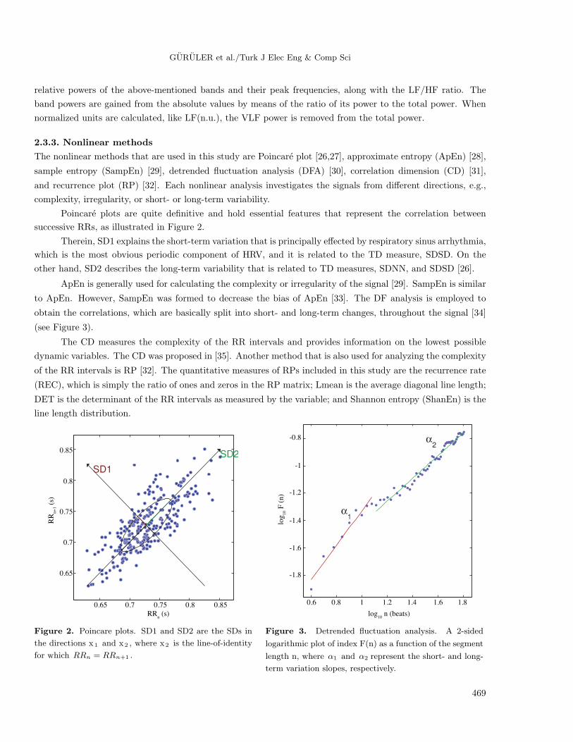
Poincare plots are quite definitive and hold essential features that represent the correlation between

successive RRs, as illustrated in Figure 2.

Therein, SD1 explains the short-term variation that is principally effected by respiratory sinus arrhythmia,

which is the most obvious periodic component of HRV, and it is related to the TD measure, SDSD. On the

other hand, SD2 describes the long-term variability that is related to TD measures, SDNN, and SDSD [26].

ApEn is generally used for calculating the complexity or irregularity of the signal [29]. SampEn is similar

to ApEn. However, SampEn was formed to decrease the bias of ApEn [33]. The DF analysis is employed to

obtain the correlations, which are basically split into short- and long-term changes, throughout the signal [34]

(see Figure 3).

The CD measures the complexity of the RR intervals and provides information on the lowest possible

dynamic variables. The CD was proposed in [35]. Another method that is also used for analyzing the complexity

of the RR intervals is RP [32]. The quantitative measures of RPs included in this study are the recurrence rate

(REC), which is simply the ratio of ones and zeros in the RP matrix; Lmean is the average diagonal line length;

DET is the determinant of the RR intervals as measured by the variable; and Shannon entropy (ShanEn) is the

line length distribution.

0.85

0.85

RRn (s)

RR

n+

1 (

s)

0.8

0.8

0.75

0.75

0.7

0.7

0.65

0.65

-0.8

-1

-1.2

-1.4

-1.6

-1.8

0.6 0.8 1 1.41.2 1.6 1.8

log10

n (beats)

log

10 F

(n

)

Figure 2. Poincare plots. SD1 and SD2 are the SDs in

the directions x1 and x2 , where x2 is the line-of-identity

for which RRn = RRn+1 .

Figure 3. Detrended fluctuation analysis. A 2-sided

logarithmic plot of index F(n) as a function of the segment

length n, where α1 and α2 represent the short- and long-

term variation slopes, respectively.

469

GURULER et al./Turk J Elec Eng & Comp Sci

2.4. Feature selection

This study uses the automatic feature selection mechanism that selects better combinations from a variety of

HRV parameters based on the CMs. After obtaining all of the HRV feature parameters involving time, frequency

(FFT and AR), and nonlinear analysis, the following steps are followed:

• Calculate the CC value of every single feature parameter regarding the target column.

• Weigh the features as they correlate to the target and establish a weighting scale.

• Compute the mean value for each group.

• Sort the input scores in descending order.

• Select the parameters having CCs that are larger than the mean value of each group, regardless of their

polarity.

• Carry the selected parameters as inputs to the NN classifiers.

2.5. The structure of the NN

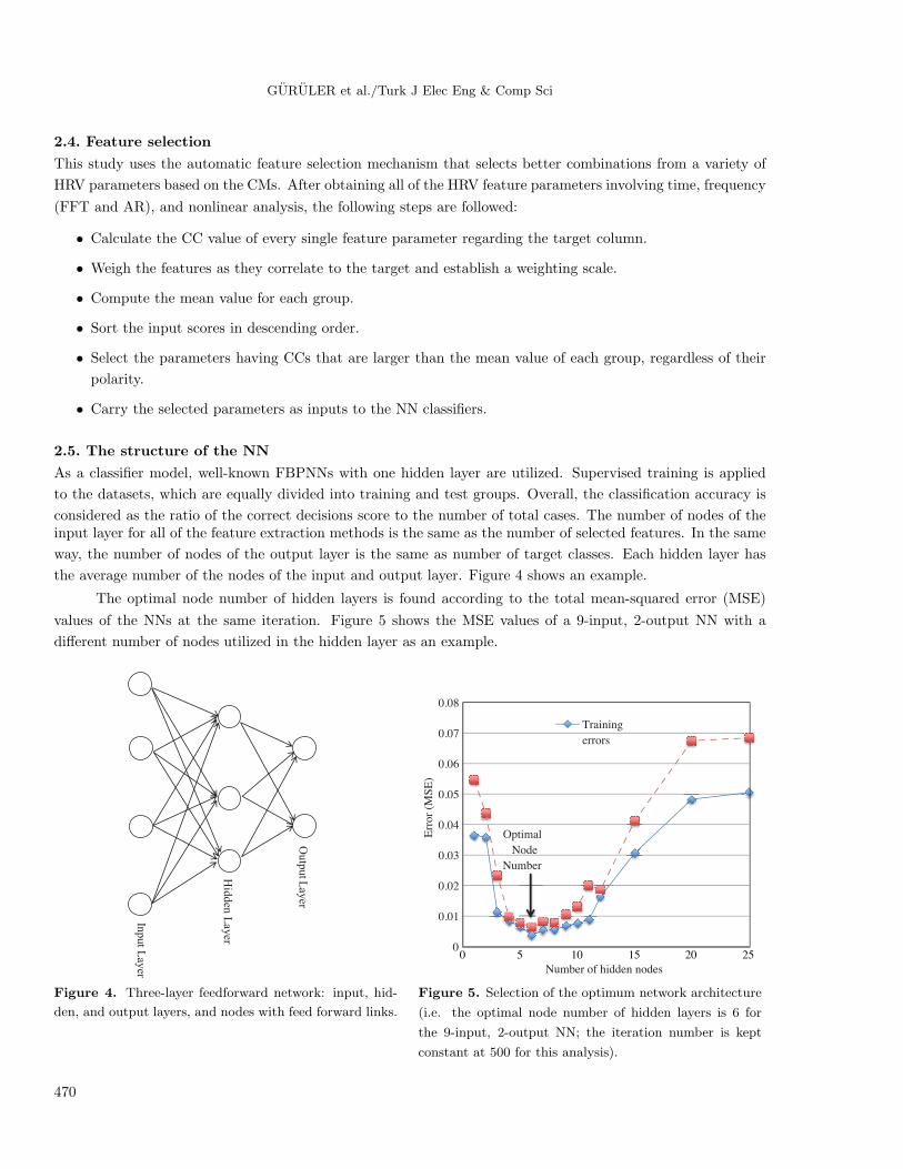
As a classifier model, well-known FBPNNs with one hidden layer are utilized. Supervised training is applied

to the datasets, which are equally divided into training and test groups. Overall, the classification accuracy is

considered as the ratio of the correct decisions score to the number of total cases. The number of nodes of theinput layer for all of the feature extraction methods is the same as the number of selected features. In the same

way, the number of nodes of the output layer is the same as number of target classes. Each hidden layer has

the average number of the nodes of the input and output layer. Figure 4 shows an example.

The optimal node number of hidden layers is found according to the total mean-squared error (MSE)

values of the NNs at the same iteration. Figure 5 shows the MSE values of a 9-input, 2-output NN with a

different number of nodes utilized in the hidden layer as an example.

Outp

ut L

ayer

Hid

den

Layer

Input L

ayer

0

0.01

0.02

0.03

0.04

0.05

0.06

0.07

0.08

Err

or

(MS

E)

Number of hidden nodes

Training

errors

Optimal

Node

Number

0 5 10 15 20 25

Figure 4. Three-layer feedforward network: input, hid-

den, and output layers, and nodes with feed forward links.

Figure 5. Selection of the optimum network architecture

(i.e. the optimal node number of hidden layers is 6 for

the 9-input, 2-output NN; the iteration number is kept

constant at 500 for this analysis).

470

GURULER et al./Turk J Elec Eng & Comp Sci

This experimentally decided optimal approach introduces a higher level of objectivity while comparing

the relations between input features and output classes, and also keeps the same structure of the NNs utilized

for different classification processes. Table 2 includes the input, hidden, and output layer sizes of the NNs of

the applied methods.

Table 2. The number of nodes in the input, hidden, and output layers used in the FBPNNs.

Feature setsNumber of nodesInput layer Hidden layer Output layer*

1. Only highly correlated (OHC) temporal parameters 5 4 2 or 32. OHC FFT spectral parameters 5 4 2 or 33. OHC AR spectral parameters 6 4 2 or 34. OHC nonlinear parameters 6 4 2 or 35. All parameters, including from 1 to 4 21 12 2 or 36. The parameters selected as OHC from 1 to 4 9 6 2 or 3

*: In the classification of ‘apnea’ and ‘healthy’ only, the number of output layers is 2. In the classification of ‘apnea’,

‘hypopnea’, and ‘healthy’, the number of output layers is 3.

The hyperbolic tangent sigmoid (tansig) transfer function is used for NNs. According to one study [36],

the hyperbolic tangent function performs better recognition accuracy than those of the other transfer functions.

This has been tested on MLPANNs, having the same iteration numbers and the same number of neurons in the

hidden layer, with 5 different activation functions. Eq. (1) gives its function, and Figure 6 gives its graphical

definitions.

tan sig (n) =2

1 + e−2n− 1 (1)

a

+1

n

-1

0

a = tansig (n)

Figure 6. Transfer function graph.

2.6. Results

In this study, a high variety of HRV features are considered. In order to recognize the normal and disease

conditions, the feature selection process is utilized on the classifier parameters. CMs are created with the

parameters obtained from the temporal, frequency, and nonlinear parameters of the HRV presented in the

tables. Table 3 gives the CMs of the TD HRV parameters used in the study.

In Table 2, pNN50, which defines 34% accuracy of the differentiation by this parameter alone, is the most

important feature in the TD analysis. The mean HR is the negative maximum. The mean value of the temporal

parameters is 0.177047, nearly half of the maximum value. Normally, the SD parameters’ CCs (SDRR, SDHR,

471

GURULER et al./Turk J Elec Eng & Comp Sci

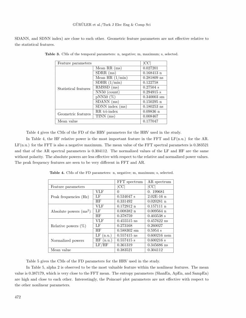
SDANN, and SDNN index) are close to each other. Geometric feature parameters are not effective relative to

the statistical features.

Table 3. CMs of the temporal parameters: n, negative; m, maximum; s, selected.

Feature parameters |CC|

Statistical features

Mean RR (ms) 0.027201SDRR (ms) 0.168413 nMean HR (1/min) 0.281809 nsSDHR (1/min) 0.122758RMSSD (ms) 0.27504 sNN50 (count) 0.294915 spNN50 (%) 0.340003 smSDANN (ms) 0.150295 nSDNN index (ms) 0.180253 ns

Geometric featuresRR tri-index 0.09836 nTINN (ms) 0.008467

Mean value 0.177047

Table 4 gives the CMs of the FD of the HRV parameters for the HRV used in the study.

In Table 4, the HF relative power is the most important feature in the FFT and LF(n.u.) for the AR.

LF(n.u.) for the FFT is also a negative maximum. The mean value of the FFT spectral parameters is 0.383521

and that of the AR spectral parameters is 0.304112. The normalized values of the LF and HF are the same

without polarity. The absolute powers are less effective with respect to the relative and normalized power values.

The peak frequency features are seen to be very different in FFT and AR.

Table 4. CMs of the FD parameters: n, negative; m, maximum; s, selected.

FFT spectrum AR spectrumFeature parameters |CC| |CC|

Peak frequencies (Hz)

VLF 0 0. 199681LF 0.534047 s 2.02E-16 nHF 0.331492 0.020281 n

Absolute powers (ms2)

VLF 0.172912 n 0.157111 nLF 0.008382 n 0.009564 nHF 0.378759 0.403538 s

Relative powers (%)

VLF 0.455515 ns 0.457622 nsLF 0.273168 0.260027HF 0.588302 sm 0.5954 s

Normalized powers

LF (n.u.) 0.557415 ns 0.600216 nsmHF (n.u.) 0.557415 s 0.600216 sLF/HF 0.361319 0.345686 ns

Mean value 0.383521 0.304112

Table 5 gives the CMs of the FD parameters for the HRV used in the study.

In Table 5, alpha 2 is observed to be the most valuable feature within the nonlinear features. The mean

value is 0.387179, which is very close to the FFT mean. The entropy parameters (ShanEn, ApEn, and SampEn)

are high and close to each other. Interestingly, the Poincare plot parameters are not effective with respect to

the other nonlinear parameters.

472

GURULER et al./Turk J Elec Eng & Comp Sci

In Tables 3–5, each parameter has a CC value that describes a predictability of the classification

numerically; the parameters with predictivities less than the mean CC values are eliminated, and from those

having equal CC values, only one is taken and the polarity of the correlation is not considered. In Tables 3–5,

the negative, maximum, and selected parameters’ CC values are denoted by n, m, and s, respectively. Tables

2–4 show that the mean values of the nonlinear and FD features are almost the same and twice as high with

respect to the temporal features. This rule also applies to the maximum values.

Figure 7A shows the classification and 7B shows the iteration results.

(a) (b)

0.63

0.78 0.78 0.72

0.78 0.82

0.85

0.93 0.93 0.96 0.96 0.96

0

0.2

0.4

0.6

0.8

1

1 2 3 4 5 6

A

- C

lass

ific

atio

n A

ccura

cy

Methods

100

500

300

400

600 600

60

300

70 100

50

0

100

200

300

400

500

600

1 2 3 4 5 6

B -

Ite

rati

on N

um

ber

s

Methods

Seri 1 Seri 2

Figure 7. A) Classification and B) iteration results. Classes: A, apnea; B, hypopnea; C, healthy. Series: 1) results for

2 classes, A+B and C; 2) results for 3 classes: A, B, and C. Methods: 1) only highly correlated temporal parameters;

2) only highly correlated FFT spectral parameters; 3) only highly correlated AR spectral parameters; 4) only highly

correlated nonlinear parameters; 5) all parameters including those from methods 1 to 4; 6) the parameters selected as

only highly correlated from methods 1 to 4.

Table 5. CMs of the nonlinear parameters: n, negative; m, maximum; s, selected.

Feature parameters |CC|

Poincare plotSD1 (ms) 0.275041SD2 (ms) 0.173002 n

RPA

Mean line length (beats) 0.174557 nMax line length (beats) 0.569607 nsREC (%) 0.159749 nDET (%) 0.586488 nsShanEn 0.367369 n

DFAalpha 1 0.556607 nsalpha 2 0.634889 nsm

Others

ApEn 0.441549 sSampEn 0.453813 sCD 0.253476

Mean value 0.387179

It can be seen from Figure 7A that the accuracy is ranked from high to low using the parameters of

nonlinear, frequency, and TD, respectively. The accuracy is 96% for the classification of A and C (A: apnea, C:

healthy) and 82% for the classification of A, B, and C (A: apnea, B: hypopnea, C: healthy), respectively.

An unexpected low accuracy is observed for the classification of A, B, and C using method 4. The other

methods correlate to the input parameters’ effectiveness, which are seen in Tables 3–5. Methods 4, 5, and 6

473

GURULER et al./Turk J Elec Eng & Comp Sci

produced the same accuracy for the classification of A and C. However, the iterations are nearly twice as high.

The iteration numbers are very high for the classification of A, B, and C (see Figure 7B).

3. Discussion and conclusions

The presented study offers a feature selection method to optimize classifier performance by means of realizing

the classification task more accurately in a shorter time. The analysis is realized on a variety of features

obtained from the time, spectral, and nonlinear components of heartbeat intervals. The results related to the

performed accuracies with the dimension reduction on the feature sets clearly show that the CMs can be focused

on reducing the feature sets and discarding the insignificant or less important features, along with being used

for any type of diagnosis by numerically determining what features better represent the targeted disorder.

As a similar study in many aspects, Gunes et al. [37] proposed a new feature selection method called

multiclass f-score feature selection combined with a multilayer perceptron artificial NN (MLPANN) in the

classification of OSA. They used the clinical features obtained from a PSG device as a diagnostic tool for OSA

in patients clinically suspected of suffering from this disease in order to determine the features related to OSA.

These clinical features were the arousal index, AHI, SaO2 minimum value in a stage of rapid eye movement,

and the percent sleep time in a stage of SaO2 intervals larger than 90%. The study selected the same features

as in our study, and only the features that were bigger than the mean value were used in the classification.

While the MLPANN obtained 63.41% classification accuracy in the diagnosis of OSA, the combination of the

MLPANN and multiclass f-score feature selection achieved 84.14%.

Two studies [38,39] presented another example of an automated diagnostic system to feature selection

combined with a NN to improve classifier accuracy. This diagnostic system consisted of a combined fuzzy

clustering NN algorithm. The results demonstrated that the proposed diagnostic systems achieved a high

(99%) accuracy rate.

Based on the results of this study, and looking at the other studies that used the same

Apnea-ECG database, the following can be concluded:

Six studies [40–45] made use of a spectral analysis of HRV. Two studies [40,46] employed the Hilbert

transform to obtain spectral information of the HR. Three algorithms [40–42] used time-frequency maps of the

HRV. In all of the FD techniques, the spectral power in the 0.01–0.04 Hz range was identified as an important

parameter. Algorithms using a FD analysis received better results than those using a TD analysis, as in the

present study. However, there were also some successful methods based on TD parameters. One approach

utilized the time measurements of HRV with some nonlinear parameters [47] and the other TD method used

rules implemented by a human administration for defining the periodic variation of the HR [48] to improve their

results.

In some studies, several ECG-derived parameters different from HRV parameters were also used to

diagnose, such as ECG pulse energy [41], R-wave duration [45], amplitude value of the S wave of each QRS [41],

and ECG-derived respiration. The selected FD parameters with the R-wave morphology gave better results.

Acknowledgments

We would like to express gratitude to the Scientific and Technological Research Council of Turkey (TUBITAK).

Huseyin Guruler was awarded a grant by TUBITAK. The grant number, name, and season are 2214-International

Research Fellowship Program 2009/2.

474

GURULER et al./Turk J Elec Eng & Comp Sci

References

[1] O. Sayadi, M.B. Shamsollahi, G.D. Clifford, “Synthetic ECG generation and Bayesian filtering using a Gaussian

wave-based dynamical model”, Physiological Measurement, Vol. 31, pp. 1309–1329, 2010.

[2] S.M.K. Jos, A.E. Spaan, Advances in Cardiac Signal Processing, Berlin, Springer-Verlag, 2007.

[3] H. Abdullah, N.C. Maddage, I. Cosic, D. Cvetkovic, “Cross-correlation of EEG frequency bands and heart rate

variability for sleep apnoea classification”, Medical & Biological Engineering & Computing, Vol. 48, pp. 1261–1269,

2010.

[4] M.J. Lado, X.A. Vila, L. Rodriguez-Linares, A.J. Mendez, D.N. Olivieri, P. Felix, “Detecting sleep apnea by heart

rate variability analysis: assessing the validity of databases and algorithms”, Journal of Medical Systems, Vol. 4,

pp. 473–481, 2009.

[5] F. Roche, S. Celle, V. Pichot, J.C. Barthelemy, E. Sforza, “Analysis of the interbeat interval increment to detect

obstructive sleep apnoea/hypopnoea”, European Respiratory Journal, Vol. 29, pp. 1206–1211, 2007.

[6] B. Yilmaz, M.H. Asyali, E. Arikan, S. Yetkin, F. Ozgen, “Sleep stage and obstructive apneaic epoch classification

using single-lead ECG”, Biomedical Engineering Online, Vol. 9, pp. 39, 2010.

[7] P. de Chazal, C. Heneghan, E. Sheridan, R. Reilly, P. Nolan, M. O’Malley, “Automated processing of the single-lead

electrocardiogram for the detection of obstructive sleep apnoea”, IEEE Transactions on Biomedical Engineering,

Vol. 50, pp. 686–696, 2003.

[8] C. O’Brien, C. Heneghan, “A comparison of algorithms for estimation of a respiratory signal from the surface

electrocardiogram”, Computers in Biology and Medicine, Vol. 37, pp. 305–314, 2007.

[9] M.O. Mendez, D.D. Ruini, O.P. Villantieri, M. Matteucci, T. Penzel, S. Cerutti, A.M. Bianchi, “Detection of sleep

apnea from surface ECG based on features extracted by an autoregressive model”, Conference Proceedings of the

IEEE Engineering in Medicine and Biology Society, Vol. 2007, pp. 6106–6109, 2007.

[10] E. Sforza, S. Grandin, C. Jouny, T. Rochat, V. Ibanez, “Is waking electroencephalographic activity a predictor

of daytime sleepiness in sleep-related breathing disorders?”, European Respiratory Journal, Vol. 19, pp. 645–652,

2002.

[11] D. Alvarez, R. Hornero, J.V. Marcos, F. del Campo, “Multivariate analysis of blood oxygen saturation recordings

in obstructive sleep apnea diagnosis”, IEEE Transactions on Biomedical Engineering, Vol. 57, pp. 2816–2824, 2010.

[12] E. Goldshtein, A. Tarasiuk, Y. Zigel, “Automatic detection of obstructive sleep apnea using speech signals”, IEEE

Transactions on Biomedical Engineering, Vol. 58, pp. 1373–1382, 2011.

[13] T. Penzel, J. McNames, A. Murray, P. de Chazal, G. Moody, B. Raymond, “Systematic comparison of different

algorithms for apnoea detection based on electrocardiogram recordings”, Medical & Biological Engineering &

Computing, Vol. 40, pp. 402–407, 2002.

[14] M.F. Hilton, R.A. Bates, K.R. Godfrey, M.J. Chappell, R.M. Cayton, “Evaluation of frequency and time-frequency

spectral analysis of heart rate variability as a diagnostic marker of the sleep apnoea syndrome”, Medical & Biological

Engineering & Computing, Vol. 37, pp. 760–769, 1999.

[15] F. Roche, J.M. Gaspoz, I. Court-Fortune, P. Minini, V. Pichot, D. Duverney, F. Costes, J.R. Lacour, J.C.

Barthelemy, “Screening of obstructive sleep apnea syndrome by heart rate variability analysis”, Circulation, Vol.

100, pp. 1411–1415, 1999.

[16] J. Corthout, S. Van Huffel, M.O. Mendez, A.M. Bianchi, T. Penzel, S. Cerutti, “Automatic screening of obstructive

sleep apnea from the ECG based on empirical mode decomposition and wavelet analysis”, Proceedings of the

30th Annual International Conference of the IEEE Engineering in Medicine and Biology Society, Vol. 2008, pp.

3608–3611, 2008.

[17] M.O. Mendez, J. Corthout, S. Van Huffel, M. Matteucci, T. Penzel, S. Cerutti, A.M. Bianchi, “Automatic

screening of obstructive sleep apnea from the ECG based on empirical mode decomposition and wavelet analysis”,

Physiological Measurement, Vol. 31, pp. 273–289, 2010.

475

GURULER et al./Turk J Elec Eng & Comp Sci

[18] U.R. Acharya, K.P. Joseph, N. Kannathal, C.M. Lim, J.S. Suri, “Heart rate variability: a review”, Medical and

Biological Engineering and Computing, Vol. 44, pp. 1031–1051, 2006.

[19] A.F. Quiceno-Manrique, J.B. Alonso-Hernandez, C.M. Travieso-Gonzalez, M. A. Ferrer-Ballester, G. Castellanos-

Dominguez, “Detection of obstructive sleep apnea in ECG recordings using time-frequency distributions and

dynamic features”, Conference Proceedings of the IEEE Engineering in Medicine and Biology Society, Vol. 2009,

pp. 5559–5562, 2009.

[20] M.A. Al-Abed, M. Manry, J.R. Burk, E.A. Lucas, K. Behbehani, “Sleep disordered breathing detection using heart

rate variability and R-peak envelope spectrogram”, Conference Proceedings of the IEEE Engineering in Medicine

and Biology Society, Vol. 2009, pp. 7106–7109, 2009.

[21] G.B. Moody, R.G. Mark, A.L. Goldberger, T. Penzel, “Stimulating rapid research advances via focused competition:

the computers in cardiology challenge 2000”, Computers in Cardiology 2000, pp. 207–210, 2000.

[22] T. Penzel, G.B. Moody, R.G. Mark, A.L. Goldberger, J.H. Peter, “Apnea-ECG database”, Computers in Cardiology

2000, Vol. 27, pp. 255–258, 2000.

[23] W.R. Ruehland, P.D. Rochford, F.J. O’Donoghue, R.J. Pierce, P. Singh, A.T. Thornton, “The new AASM criteria

for scoring hypopneas: impact on the apnea hypopnea index”, Sleep, Vol. 32, pp. 150–157, 2009.

[24] J.P. Niskanen, M.P. Tarvainen, P.O. Ranta-Aho, P.A. Karjalainen, “Software for advanced HRV analysis”, Computer

Methods and Programs in Biomedicine, Vol. 76, pp. 73–81, 2004.

[25] A.J. Camm, M. Malik, J.T. Bigger, G. Breithardt, S. Cerutti, R.J. Cohen, P. Coumel, E.L. Fallen, H.L. Kennedy,

R.E. Kleiger, F. Lombardi, A. Malliani, A.J. Moss, J.N. Rottman, G. Schmidt, P.J. Schwartz, D.H. Singer, “Heart

rate variability: standards of measurement, physiological interpretation and clinical use. Task Force of the European

Society of Cardiology and the North American Society of Pacing and Electrophysiology”, Circulation, Vol. 93, pp.

1043–1065, 1996.

[26] M. Brennan, M. Palaniswami, P. Kamen, “Do existing measures of Poincare plot geometry reflect nonlinear features

of heart rate variability?”, IEEE Transactions on Biomedical Engineering, Vol. 48, pp. 1342–1347, 2001.

[27] S. Carrasco, M.J. Gaitan, R. Gonzalez, O. Yanez, “Correlation among Poincare plot indexes and time and frequency

domain measures of heart rate variability”, Journal of Medical Engineering and Technology, Vol. 25, pp. 240–248,

2001.

[28] J.S. Richman, J.R. Moorman, “Physiological time-series analysis using approximate entropy and sample entropy”,

American Journal of Physiology-Heart and Circulatory Physiology, Vol. 278, pp. 2039–2049, 2000.

[29] H.B.Y. Fusheng, T. Qingyu, “Approximate entropy and its application in biosignal analysis”, in M. Akay, editor,

Nonlinear Biomedical Signal Processing: Dynamic Analysis and Modeling, Vol. 2, New York, IEEE Press, pp. 72–91,

2001.

[30] C.K. Peng, S. Havlin, H.E. Stanley, A.L. Goldberger, “Quantification of scaling exponents and crossover phenomena

in nonstationary heartbeat time-series”, Chaos, Vol. 5, pp. 82–87, 1995.

[31] S. Guzzetti, M.G. Signorini, C. Cogliati, S. Mezzetti, A. Porta, S. Cerutti, A. Malliani, “Non-linear dynamics

and chaotic indices in heart rate variability of normal subjects and heart-transplanted patients”, Cardiovascular

Research, Vol. 31, pp. 441–446, 1996.

[32] C.L. Webber, J.P. Zbilut, “Dynamical assessment of physiological systems and states using recurrence plot strate-

gies”, Journal of Applied Physiology, Vol. 76, pp. 965–973, 1994.

[33] D.E. Lake, J.S. Richman, M.P. Griffin, J.R. Moorman, “Sample entropy analysis of neonatal heart rate variability”,

American Journal of Physiology-Regulatory Integrative and Comparative Physiology, Vol. 283, pp. R789–R797,

2002.

[34] T. Penzel, J.W. Kantelhardt, L. Grote, J.H. Peter, A. Bunde, “Comparison of detrended fluctuation analysis and

spectral analysis for heart rate variability in sleep and sleep apnea”, IEEE Transactions on Biomedical Engineering,

Vol. 50, pp. 1143–1151, 2003.

476

GURULER et al./Turk J Elec Eng & Comp Sci

[35] P. Grassberger, I. Procaccia, “Characterization of strange attractors”, Physical Review Letters, Vol. 50, pp. 346–349,

1983.

[36] B. Karlik, A.V. Olgac, “Performance analysis of various activation functions in generalized MLP architectures of

neural networks”, International Journal of Artificial Intelligence and Expert Systems, Vol. 1, pp. 111–122, 2011.

[37] S. Gunes, K. Polat, S. Yosunkaya, “Multi-class f-score feature selection approach to classification of obstructive

sleep apnea syndrome”, Expert Systems with Applications, Vol. 37, pp. 998–1004, 2010.

[38] Y. Ozbay, R. Ceylan, B. Karlik, “A fuzzy clustering neural network architecture for classification of ECG arrhyth-

mias”, Computers in Biology and Medicine, Vol. 36, pp. 376–388, 2006.

[39] R. Ceylan, Y. Ozbay, B. Karlik, “A novel approach for classification of ECG arrhythmias: type-2 fuzzy clustering

neural network”, Expert Systems with Applications, Vol. 36, pp. 6721–6726, 2009.

[40] M. Schrader, C. Zywietz, V. von Einem, B. Widiger, G. Joseph, “Detection of sleep apnea in single channel ECGs

from the Physionet data base”, Computers in Cardiology 2000, Vol. 27, pp. 263–266, 2000.

[41] J.N. McNames, A.M. Fraser, “Obstructive sleep apnea classification based on spectrogram patterns in the electro-

cardiogram”, Computers in Cardiology 2000, Vol. 27, pp. 749–752, 2000.

[42] M.R. Jarvis, P.P. Mitra, “Apnea patients characterized by 0.02 Hz peak in the multitaper spectrogram of electro-

cardiogram signals”, Computers in Cardiology 2000, Vol. 27, pp. 769–772, 2000.

[43] M.J. Drinnan, J. Allen, P. Langley, A. Murray, “Detection of sleep apnoea from frequency analysis of heart rate

variability”, Computers in Cardiology 2000, Vol. 27, pp. 259–262, 2000.

[44] P. de Chazal, C. Heneghan, E. Sheridan, R. Reilly, P. Nolan, M. O’Malley, “Automatic classification of sleep apnea

epochs using the electrocardiogram”, Computers in Cardiology 2000, Vol. 27, pp. 745–748, 2000.

[45] Z. Shinar, A. Baharav, S. Akselrod, “Obstructive sleep apnea detection based on electrocardiogram analysis”,

Computers in Cardiology 2000, Vol. 27, pp. 757–760, 2000.

[46] J.E. Mietus, C.K. Peng, P.C. Ivanov, A.L. Goldberger, “Detection of obstructive sleep apnea from cardiac interbeat

interval time series”, Computers in Cardiology 2000, Vol. 27, pp. 753–756, 2000.

[47] C. Maier, M. Bauch, H. Dickhaus, “Recognition and quantification of sleep apnea by analysis of heart rate variability

parameters”, Computers in Cardiology 2000, Vol. 27, pp. 741–744, 2000.

[48] P.K. Stein, P.P. Domitrovich, “Detecting OSAHS from patterns seen on heart-rate tachograms”, Computers in

Cardiology 2000, Vol. 27, pp. 271–274, 2000.

477

GURULER et al./Turk J Elec Eng & Comp Sci

Appendix. Summary of the HRV measures.

478