Feature Engineering and Selection - Peoplejordan/courses/294-fall09/... · Feature Engineering and Selection CS 294: Practical Machine Learning October 1st, 2009 Alexandre Bouchard-Côté

Feature Engineering and Selection

CS 294: Practical Machine LearningOctober 1st, 2009

Alexandre Bouchard-Côté

Abstract supervised setup• Training : • : input vector

• y : response variable– : binary classification– : regression– what we want to be able to predict, having

observed some new .

xi =

!

"""#

xi,1

xi,2...

xi,n

$

%%%&, xi,j ! R

Concrete setup

“Danger”

Input Output

!

"""#

xi,1

xi,2...

xi,n

$

%%%&

Featurization

“Danger”

Input OutputFeatures

!

"""#

xi,1

xi,2...

xi,n

$

%%%&

Outline

• Today: how to featurize effectively– Many possible featurizations– Choice can drastically affect performance

• Program:– Part I : Handcrafting features: examples, bag

of tricks (feature engineering)– Part II: Automatic feature selection

Part I: Handcrafting Features

Machines still need us

Example 1: email classification

• Input: a email message• Output: is the email...

– spam,– work-related,– personal, ...

PERSONAL

• Input: (email-valued)• Feature vector:

• Learn one weight vector for each class:

• Decision rule:

Basics: bag of wordsx

f(x) =

!

"""#

f1(x)f2(x)

...fn(x)

$

%%%&, e.g. f1(x) =

'1 if the email contains “Viagra”0 otherwise

Indicator or Kronecker

delta function

y = argmaxy!wy, f(x)"

wy ! Rn, y ! {SPAM,WORK,PERS}

Feature vector hashtable

extractFeature(Email e) {

result <- hashtable

for (String word : e.getWordsInBody()) result.put("UNIGRAM:" + word, 1.0) String previous = "#" for (String word : e.getWordsInBody()) { result.put("BIGRAM:"+ previous + " " + word, 1.0) previous = word }

return result }

f(x)

Implementation: exploit sparsity

Feature template 1:UNIGRAM:Viagra

Feature template 2:BIGRAM:Cheap Viagra

• Each user inbox is a separate learning problem – E.g.: Pfizer drug designer’s inbox

• Most inbox has very few training instances, but all the learning problems are clearly related

Features for multitask learning

• Solution: include both user-specific and global versions of each feature. E.g.:– UNIGRAM:Viagra– USER_id4928-UNIGRAM:Viagra

• Equivalent to a Bayesian hierarchy under some conditions (Finkel et al. 2009)

Features for multitask learning [e.g.:Daumé 06]

x x

y y

w w

w

User

1

User

2

...

• In multiclass classification, output space often has known structure as well

• Example: a hierarchy:

Structure on the output space

Emails

Spam Ham

Advance fee frauds

Spamvertised sites

Backscatter Work

Mailing lists

Personal

• Slight generalization of the learning/prediction setup: allow features to depend both on the input x and on the class y

w ! Rm,

y = argmaxy!w, f(x, y)"


Before: • One weight/class:

• Decision rule:

wy ! Rn,

y = argmaxy!wy, f(x)"

After: • Single weight:

• New rule:

• At least as expressive: conjoin each feature with all output classes to get the same model

• E.g.: UNIGRAM:Viagra becomes– UNIGRAM:Viagra AND CLASS=FRAUD– UNIGRAM:Viagra AND CLASS=ADVERTISE– UNIGRAM:Viagra AND CLASS=WORK– UNIGRAM:Viagra AND CLASS=LIST– UNIGRAM:Viagra AND CLASS=PERSONAL


Exploit the information in the hierarchy by activating both coarse and fine versions of the features on a given input:


...UNIGRAM:Alex AND CLASS=PERSONALUNIGRAM:Alex AND CLASS=HAM ...

Emails

Spam Ham

Advance

fee frauds

Spamvertised

sites

Backscatter Work

Mailing lists

Personal

x y


• Not limited to hierarchies– multiple hierarchies– in general, arbitrary featurization of the output

• Another use: – want to model that if no words in the email

were seen in training, it’s probably spam– add a bias feature that is activated only in

SPAM subclass (ignores the input): CLASS=SPAM

Dealing with continuous data

• Full solution needs HMMs (a sequence of correlated classification problems): Alex Simma will talk about that on Oct. 15

• Simpler problem: identify a single sound unit (phoneme)

“Danger”

“r”

Dealing with continuous data• Step 1: Find a coordinate system where

similar input have similar coordinates– Use Fourier transforms and knowledge

about the human ear

Time domain:

Sound 2Sound 1

Frequency domain:

Sriram Sankararaman Clustering

Dealing with continuous data• Step 2 (optional): Transform the

continuous data into discrete data– Bad idea: COORDINATE=(9.54,8.34)– Better: Vector quantization (VQ)

– Run k-mean on the training data as a preprocessing step

– Feature is the index of the nearest centroidCLUSTER=1

CLUSTER=2

Dealing with continuous dataImportant special case: integration of the output of a black box – Back to the email classifier: assume we

have an executable that returns, given a email e, its belief B(e) that the email is spam

– We want to model monotonicity– Solution: thermometer feature

B(e) > 0.8 AND CLASS=SPAM

B(e) > 0.6 AND CLASS=SPAM

B(e) > 0.4 AND CLASS=SPAM... ...

fi(x, y) =!

log B(e) if y = SPAM0 otherwise

Dealing with continuous data

Another way of integrating a qualibrated black box as a feature:

Recall: votes are combined

additively

Part II: (Automatic) Feature Selection

What is feature selection?• Reducing the feature space by throwing

out some of the features• Motivating idea: try to find a simple,

“parsimonious” model– Occam’s razor: simplest explanation that

accounts for the data is best

What is feature selection?

UNIGRAM:Viagra 0

UNIGRAM:the 1BIGRAM:the presence 0BIGRAM:hello Alex 1UNIGRAM:Alex 1UNIGRAM:of 1BIGRAM:absence of 0BIGRAM:classify email 0BIGRAM:free Viagra 0BIGRAM:predict the 1

…BIGRAM:emails as 1

UNIGRAM:Viagra 0BIGRAM:hello Alex 1BIGRAM:free Viagra 0

Vegetarian NoPlays video games

Yes

Family history NoAthletic NoSmoker YesGender MaleLung capacity 5.8LHair color RedCar Audi…

Weight 185 lbs

Family history

No

Smoker Yes

Task: classify emails as spam, work, ...

Data: presence/absence of words

Task: predict chances of lung disease

Data: medical history survey

X X

Reduced XReduced X

Outline• Review/introduction

– What is feature selection? Why do it?• Filtering• Model selection

– Model evaluation– Model search

• Regularization• Summary recommendations

Why do it?• Case 1: We’re interested in features—we want

to know which are relevant. If we fit a model, it should be interpretable.

• Case 2: We’re interested in prediction; features are not interesting in themselves, we just want to build a good classifier (or other kind of predictor).

Why do it? Case 1.

• What causes lung cancer? – Features are aspects of a patient’s medical history– Binary response variable: did the patient develop lung cancer?– Which features best predict whether lung cancer will develop?

Might want to legislate against these features.

• What causes a program to crash? [Alice Zheng ’03, ’04, ‘05]

– Features are aspects of a single program execution• Which branches were taken? • What values did functions return?

– Binary response variable: did the program crash?– Features that predict crashes well are probably bugs

We want to know which features are relevant; we don’t necessarily want to do prediction.

Why do it? Case 2.

• Common practice: coming up with as many features as possible (e.g. > 106 not unusual)– Training might be too expensive with all features– The presence of irrelevant features hurts generalization.

• Classification of leukemia tumors from microarray gene expression data [Xing, Jordan, Karp ’01]– 72 patients (data points)– 7130 features (expression levels of different genes)

• Embedded systems with limited resources– Classifier must be compact– Voice recognition on a cell phone– Branch prediction in a CPU

• Web-scale systems with zillions of features– user-specific n-grams from gmail/yahoo spam filters

We want to build a good predictor.

Get at Case 1 through Case 2

• Even if we just want to identify features, it can be useful to pretend we want to do prediction.

• Relevant features are (typically) exactly those that most aid prediction.

• But not always. Highly correlated features may be redundant but both interesting as “causes”.– e.g. smoking in the morning, smoking at night

Feature selection vs. Dimensionality reduction

• Removing features: – Equivalent to projecting data onto lower-dimensional linear subspace

perpendicular to the feature removed

• Percy’s lecture: dimensionality reduction – allow other kinds of projection.

• The machinery involved is very different– Feature selection can can be faster at test time– Also, we will assume we have labeled data. Some dimensionality

reduction algorithm (e.g. PCA) do not exploit this information




• Regularization• Summary

FilteringSimple techniques for weeding out irrelevant features without fitting model

Filtering• Basic idea: assign heuristic score to each

feature to filter out the “obviously” useless ones. – Does the individual feature seems to help prediction?– Do we have enough data to use it reliably? – Many popular scores [see Yang and Pederson ’97]

• Classification with categorical data: Chi-squared, information gain, document frequency

• Regression: correlation, mutual information• They all depend on one feature at the time (and the data)

• Then somehow pick how many of the highest scoring features to keep

Comparison of filtering methods for text categorization [Yang and Pederson ’97]

Filtering• Advantages:

– Very fast– Simple to apply

• Disadvantages:– Doesn’t take into account interactions between features:

Apparently useless features can be useful when grouped with others

• Suggestion: use light filtering as an efficient initial step if running time of your fancy learning algorithm is an issue





Model Selection• Choosing between possible models of

varying complexity– In our case, a “model” means a set of features

• Running example: linear regression model

Linear Regression Model

• Recall that we can fit (learn) the model by minimizing the squared error:

Input :

Response :

Parameters:

Prediction :

Least Squares Fitting(Fabian’s slide from 3 weeks ago)

0 200

Error or “residual”

Prediction

Observation

Sum squared error:

Naïve training error is misleading

• Consider a reduced model with only those features for – Squared error is now

• Is this new model better? Maybe we should compare the training errors to find out?

• Note – Just zero out terms in to match .

• Generally speaking, training error will only go up in a simpler model. So why should we use one?

Input :

Response :

Parameters:

Prediction :

Overfitting example 1

• This model is too rich for the data• Fits training data well, but doesn’t generalize.

0 2 4 6 8 10 12 14 16 18 20-15

-10

-5

0

5

10

15

20

25

30

Degree 15 polynomial

(From Fabian’s lecture)

Overfitting example 2• Generate 2000 , i.i.d.• Generate 2000 , i.i.d. completely

independent of the ’s– We shouldn’t be able to predict at all from

• Find • Use this to predict for each by

It really looks like we’ve found a relationship between and ! But no such relationship exists, so will do no better than random on new data.

Model evaluation• Moral 1: In the presence of many irrelevant

features, we might just fit noise. • Moral 2: Training error can lead us astray. • To evaluate a feature set , we need a better

scoring function • We’re not ultimately interested in training error;

we’re interested in test error (error on new data). • We can estimate test error by pretending we

haven’t seen some of our data. – Keep some data aside as a validation set. If we don’t

use it in training, then it’s a better test of our model.

K-fold cross validation• A technique for estimating test error• Uses all of the data to validate• Divide data into K groups .• Use each group as a validation set, then average all validation

errors

X1

LearnX2

X3X4

X5

X6

X7

test


errors

X1

LearnX2

X3X4

X5

X6

X7

test


errors

X1

…Learn

X2

X3X4

X5

X6

X7

test


errors

X1

LearnX2

X3X4

X5

X6

X7

Model Search

• We have an objective function – Time to search for a good model.

• This is known as a “wrapper” method– Learning algorithm is a black box– Just use it to compute objective function, then

do search• Exhaustive search expensive

– for n features, 2n possible subsets s• Greedy search is common and effective

Model search

• Backward elimination tends to find better models– Better at finding models with interacting features– But it is frequently too expensive to fit the large

models at the beginning of search• Both can be too greedy.

Backward elimination

Initialize s={1,2,…,n}Do: remove feature from s which improves K(s) mostWhile K(s) can be improved

Forward selection

Initialize s={}Do: Add feature to s which improves K(s) mostWhile K(s) can be improved

Model search• More sophisticated search strategies exist

– Best-first search– Stochastic search– See “Wrappers for Feature Subset Selection”, Kohavi and John

1997• For many models, search moves can be evaluated

quickly without refitting– E.g. linear regression model: add feature that has most

covariance with current residuals• YALE can do feature selection with cross-validation and

either forward selection or backwards elimination. • Other objective functions exist which add a model-

complexity penalty to the training error– AIC: add penalty to log-likelihood (number of features). – BIC: add penalty (n is the number of data points)





Regularization• In certain cases, we can move model

selection into the induction algorithm

• This is sometimes called an embedded feature selection algorithm

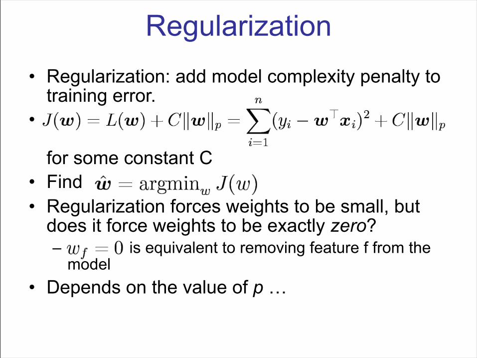
Regularization• Regularization: add model complexity penalty to

training error.•

for some constant C• Find • Regularization forces weights to be small, but

does it force weights to be exactly zero? – is equivalent to removing feature f from the

model• Depends on the value of p …

• p = 2: Euclidean

• p = 1: Taxicab or Manhattan

• General case:

p metrics and norms

||!w||2 =!

w21 + · · · + w2

n

||!w||1 = |w1| + · · · + |wn|

||!w||p = p!

|w1|p + · · · + |wn|p

0 < p ! "

Univariate case: intuitionPenalty

Featureweightvalue

Univariate case: intuitionPenalty

Featureweightvalue

L1 penalizes more than L2when the weight is small

Univariate example: L2

+ =

• Case 1: there is a lot of data supporting our hypothesis

Regularization term Data likelihoodBy itself, minimized

by w=1.1

Objective functionMinimized by

w=0.95


+ =

• Case 2: there is NOT a lot of data supporting our hypothesis


by w=1.1


w=0.36


+ =

• Case 1, when there is a lot of data supporting our hypothesis:– Almost the same resulting w as L2

• Case 2, when there is NOT a lot of data supporting our hypothesis

• Get w = exactly zero


by w=1.1


w=0.0

Level sets of L1 vs L2 (in 2D)

Weight offeature #1

Weight offeature #2

Multivariate case: w gets cornered• To minimize , we can solve

by (e.g.) gradient descent.

• Minimization is a tug-of-war between the two terms

• To minimize , we can solve by (e.g.) gradient descent.


Multivariate case: w gets cornered





• Minimization is a tug-of-war between the two terms• w is forced into the corners—components are zeroed

– Solution is often sparse


L2 does not zero components

L2 does not zero components

• L2 regularization does not promote sparsity• Even without sparsity, regularization promotes

generalization—limits expressiveness of model

Lasso Regression [Tibshirani ‘94]

• Simply linear regression with an L1 penalty for sparsity.

• Compare with ridge regression (introduced by Fabian 3 weeks ago):

w = argminw

n!

i=1

(yi !w!xi)2 + C||w||1

w = argminw

n!

i=1

(yi !w!xi)2 + C||w||22

Lasso Regression [Tibshirani ‘94]

• Simply linear regression with an L1 penalty for sparsity.

• Two questions:– 1. How do we perform this minimization?

• Difficulty: not differentiable everywhere– 2. How do we choose C?

• Determines how much sparsity will be obtained• C is called an hyperparameter

w = argminw

n!

i=1

(yi !w!xi)2 + C||w||1

Question 1: Optimization/learning• Set of discontinuity has Lebesgue

measure zero, but optimizer WILL hit them• Several approaches, including:

– Projected gradient, stochastic projected subgradient, coordinate descent, interior point, orthan-wise L-BFGS [Friedman 07, Andrew et. al. 07, Koh et al. 07, Kim et al. 07, Duchi 08]

– More on that on the John’s lecture on optimization

– Open source implementation:edu.berkeley.nlp.math.OW_LBFGSMinimizer in

http://code.google.com/p/berkeleyparser/

Question 2: Choosing C• Up until a few years ago

this was not trivial– Fitting model: optimization

problem, harder than least-squares

– Cross validation to choose C: must fit model for every candidate C value

• Not with LARS! (Least Angle Regression, Hastie et al, 2004)– Find trajectory of w for all

possible C values simultaneously, as efficiently as least-squares

– Can choose exactly how many features are wanted

Figure taken from Hastie et al (2004)

• Not to be confused: two othogonal uses of L1 for regression: – lasso for sparsity: what we just described

–L1 loss: for robustness (Fabian’s lecture).

Remarks

IntuitionPenalty

x

L1 penalizes more than L2when x is small (use this for sparsity)

L1 penalizes less than L2when x is big (use this for robustness)

• L1 penalty can be viewed as a laplace prior on the weights, just as L2 penalty can viewed as a normal prior– Side note: also possible to learn C

efficiently when the penalty is L2 (Foo, Do, Ng, ICML 09, NIPS 07)

• Not limited to regression: can be applied to classification, for example

Remarks

• For large scale problems, performance of L1 and L2 is very similar (at least in NLP)– A slight advantage of L2 over L1 in accuracy– But solution is 2 orders of magnitudes

sparser!– Parsing reranking task:

L1 Vs L2 [Gao et al ‘07]

(Higher F1is better)

• NLP example: back to the email classification task

• Zipf law: frequency of a word is inversely proportional to its frequency rank.– Fat tail: many n-grams are seen only once in

the training– Yet they can be very useful predictors – E.g. 8-gram “today I give a lecture on feature

selection” occurs only once in my mailbox, but it’s a good predictor that the email is WORK

When can feature selection hurt?





Summary: feature engineering• Feature engineering is often crucial to get

good results• Strategy: overshoot and regularize

– Come up with lots of features: better to include irrelevant features than to miss important features

– Use regularization or feature selection to prevent overfitting

– Evaluate your feature engineering on DEV set. Then, when the feature set is frozen, evaluate on TEST to get a final evaluation (Daniel will say more on evaluation next week)

Summary: feature selectionWhen should you do it?– If the only concern is accuracy, and the whole

dataset can be processed, feature selection not needed (as long as there is regularization)

– If computational complexity is critical (embedded device, web-scale data, fancy learning algorithm), consider using feature selection

• But there are alternatives: e.g. the Hash trick, a fast, non-linear dimensionality reduction technique [Weinberger et al. 2009]

– When you care about the feature themselves• Keep in mind the correlation/causation issues• See [Guyon et al., Causal feature selection, 07]

Summary: how to do feature selection•Filtering•L1 regularization (embedded methods)•Wrappers

•Forward selection•Backward selection•Other search•Exhaustive

Com

putational cost

• Good preprocessing step

• Fails to capture relationship between features

•Filtering•L1 regularization (embedded methods)•Wrappers


Com

putational cost

Summary: how to do feature selection

• Fairly efficient– LARS-type algorithms now

exist for many linear models.



Com

putational cost


• Most directly optimize prediction performance

• Can be very expensive, even with greedy search methods

• Cross-validation is a good objective function to start with



Com

putational cost


• Too greedy—ignore relationships between features

• Easy baseline• Can be generalized in

many interesting ways– Stagewise forward

selection– Forward-backward search– Boosting



Com

putational cost


• Generally more effective than greedy



Com

putational cost


• The “ideal”• Very seldom done in

practice• With cross-validation

objective, there’s a chance of over-fitting– Some subset might

randomly perform quite well in cross-validation



Com

putational cost


Extra slides

Feature engineering case study: Modeling language change [Bouchard et al. 07,09]

‘fish’ ‘fear’

Hawaiian iʔa makaʔu

Samoan iʔa mataʔu

Tongan ika

Maori ika mataku


‘fish’ ‘fear’

Hawaiian iʔa makaʔu

Samoan iʔa mataʔu

Tongan ika

Maori ika mataku

Proto-Oceanic

‘fish’ POc *ika

*k > ʔ

Tasks: • Proto-word reconstruction

• Infer sound changes


• Featurize sound changes– E.g.: substitution are generally more frequent than

insertions, deletions, changes are branch specific, but there are cross-linguistic universal, etc.

• Particularity: unsupervised learning setup– We covered feature engineering for supervised setups

for pedagogical reasons; most of what we have seen applies to the unsupervised setup

! "#

$%

&

'

(

) * +,

-

.

/

012

3

4 5

6 78

9

:

;<

=

>

?

@

f

gdb c

n

ç

m

j

k

hv

t

s

r

qp A

z

B

C x

• What is a protein? – A protein is a chain of amino acids.

• Proteins fold into a 3D conformation by minimizing energy– “Native” conformation (the one found in nature) is the lowest

energy state– We would like to find it using only computer search. – Very hard, need to try several initialization in parallel

• Regression problem: – Input: many different conformation of the same sequence– Output: energy

• Features derived from: φ and ψ torsion angles.

• Restrict next wave of search to agree with features that predicted high energy

Feature selection case study: Protein Energy Prediction [Blum et al ‘07]

Featurization• Torsion angle features can be binned

• Bins in the Ramachandran plot correspond to common structural elements– Secondary structure: alpha helices and beta sheets

φ1 ψ1 φ2 ψ2 φ3 ψ4 φ5 ψ5 φ6 ψ6

0 75.3 -61.6 -24.8 -68.6 -51.9 -63.3 -37.6 -62.8 -42.3

G A A

φ

ψ

(180, 180)

(-180, -180)

G

E

E

A

B

B

Results of LARS for predicting protein energy

• One column for each torsion angle feature• Colors indicate frequencies in data set

– Red is high, blue is low, 0 is very low, white is never– Framed boxes are the correct native features– “-” indicates negative LARS weight (stabilizing), “+”

indicates positive LARS weight (destabilizing)

Other things to check out• Bayesian methods

– David MacKay: Automatic Relevance Determination • originally for neural networks

– Mike Tipping: Relevance Vector Machines• http://research.microsoft.com/mlp/rvm/

• Miscellaneous feature selection algorithms– Winnow

• Linear classification, provably converges in the presence of exponentially many irrelevant features

– Optimal Brain Damage• Simplifying neural network structure

• Case studies– See papers linked on course webpage.

http://research.microsoft.com/mlp/rvm/

http://research.microsoft.com/mlp/rvm/

Acknowledgments• Useful comments by Mike Jordan, Percy Liang • A first version of these slides was created by Ben Blum

Documents

Feature Engineering and Selection - Peoplejordan/courses/294-fall09/... · Feature Engineering and Selection CS 294: Practical Machine Learning October 1st, 2009 Alexandre Bouchard-Côté