Embed Size (px)
Citation preview

Recursion
� Recursion occurs when a thing is defined in terms of itself.
� Recursion is an alternative form of program control.
� It is essentially repetition without loops.
Zheng-Liang Lu 185 / 383
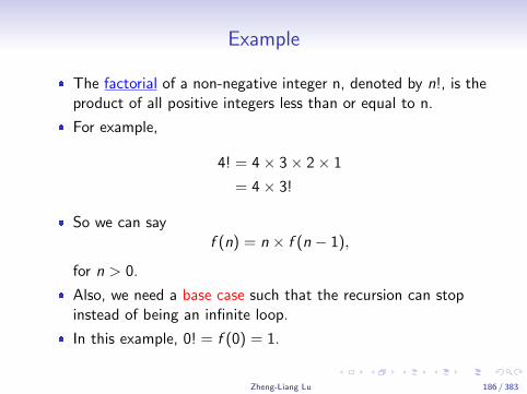
Example
� The factorial of a non-negative integer n, denoted by n!, is theproduct of all positive integers less than or equal to n.
� For example,
4! = 4× 3× 2× 1
= 4× 3!
� So we can sayf (n) = n × f (n − 1),
for n > 0.
� Also, we need a base case such that the recursion can stopinstead of being an infinite loop.
� In this example, 0! = f (0) = 1.
Zheng-Liang Lu 186 / 383

Exercise
1 function y = recursiveFactorial(n)2 if n > 03 y = n * recursiveFactorial(n - 1);4 else5 y = 1; % base case6 end7 end
Zheng-Liang Lu 187 / 383

Zheng-Liang Lu 188 / 383
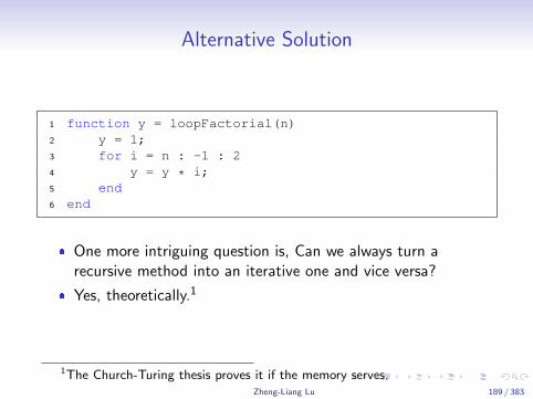
Alternative Solution
1 function y = loopFactorial(n)2 y = 1;3 for i = n : -1 : 24 y = y * i;5 end6 end
� One more intriguing question is, Can we always turn arecursive method into an iterative one and vice versa?
� Yes, theoretically.1
1The Church-Turing thesis proves it if the memory serves.Zheng-Liang Lu 189 / 383
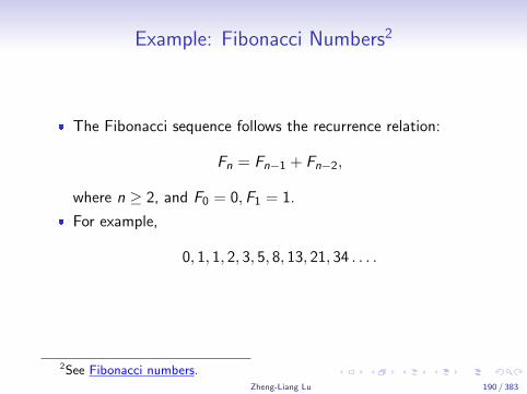
Example: Fibonacci Numbers2
� The Fibonacci sequence follows the recurrence relation:
Fn = Fn−1 + Fn−2,
where n ≥ 2, and F0 = 0,F1 = 1.
� For example,
0, 1, 1, 2, 3, 5, 8, 13, 21, 34 . . . .
2See Fibonacci numbers.Zheng-Liang Lu 190 / 383
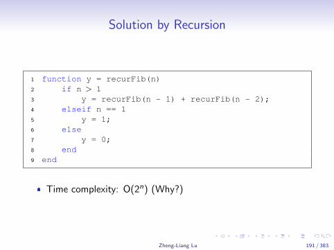
Solution by Recursion
1 function y = recurFib(n)2 if n > 13 y = recurFib(n - 1) + recurFib(n - 2);4 elseif n == 15 y = 1;6 else7 y = 0;8 end9 end
� Time complexity: O(2n) (Why?)
Zheng-Liang Lu 191 / 383
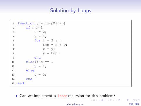
Solution by Loops
1 function y = loopFib(n)2 if n > 13 x = 0;4 y = 1;5 for i = 2 : n6 tmp = x + y;7 x = y;8 y = tmp;9 end
10 elseif n == 111 y = 1;12 else13 y = 0;14 end15 end
� Can we implement a linear recursion for this problem?
Zheng-Liang Lu 192 / 383

Solution by Linear Recursion
1 function ret = linearFib(n)2 ret = fib(0, 1, n);3 function c = fib(a, b, n) % nested function4 if n > 05 c = fib(b, b + a, n - 1);6 else7 c = a;8 end9 end
10 end
� Time complexity: O(n)!
� Actually, it can be done in O(log n) time!!3
3Seehttps://en.wikipedia.org/wiki/Fibonacci_number#Matrix_form.
Zheng-Liang Lu 193 / 383

Remarks
� Recursion bears substantial overhead.
� So the recursive algorithm may execute a bit more slowly thanthe iterative equivalent.4
� Moreover, a deeply recursive function depletes the call stackwhich is limited, and causes an exception fast.5
4In modern compiler design, recursion elimination is automatic if therecurrence occurs in the last statement in the recursive function, so called tailrecursion. However, only some of programming languages support theelimination of tail recursion. Unfortunately, Matlab does not support thisfeature.
5Aka stack overflow.Zheng-Liang Lu 194 / 383
More Interesting Recursions
� Sum of numbers
� Product of numbers
� Greatest common divisor
� Towers of Hanoi
� Check whether a string is palindrome6 using recursion
� N-Queens problem
� Quick sqrt
� Depth-first search
� Reversing a string
� Computing n mod m without using the function mod()
6For example, noon, level, and radar.Zheng-Liang Lu 195 / 383
1 >> Lecture 42 >>3 >> -- Graphics4 >>
Zheng-Liang Lu 196 / 383
Introduction
� Engineers use graphic techniques to make the informationeasier to understand.
� With graphs, it is easy to identify trends, pick out highs andlows, and isolate data points that may be measurement orcalculation errors.
� Graphs can also be used as a quick check to determinewhether a computer solution is yielding expected results.
� A set of ordered pairs is used to identify points on a 2D graph.
� The data points are then connected by piece-wise straightlines in common cases.
Zheng-Liang Lu 197 / 383

2D Line Plot
� The function plot(x , y , ’CLM’) creates a 2D line plot of thedata in y versus the corresponding values in x.
� (x , y): data set,� C: specify the color,� L: specify the line type,� M: specify the data marker.
� A figure is created automatically as soon as the function plotis called.
Zheng-Liang Lu 198 / 383

Optional Parameters for Plot7
� Try help for further details about plot.
7See http://www.mathworks.com/help/matlab/ref/plot.html.Zheng-Liang Lu 199 / 383
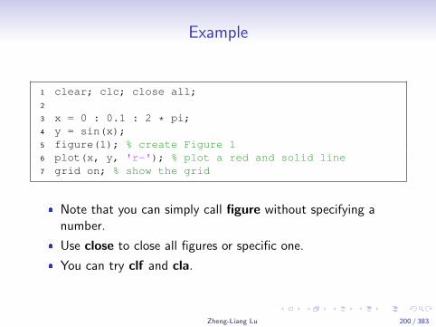
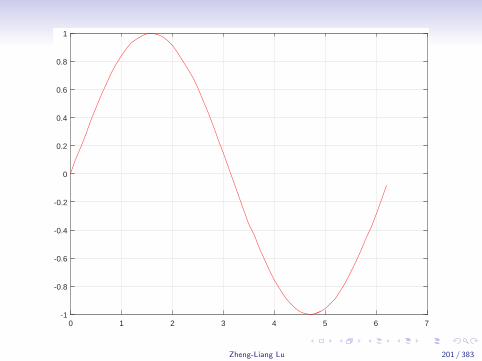
Example
1 clear; clc; close all;2
3 x = 0 : 0.1 : 2 * pi;4 y = sin(x);5 figure(1); % create Figure 16 plot(x, y, 'r-'); % plot a red and solid line7 grid on; % show the grid
� Note that you can simply call figure without specifying anumber.
� Use close to close all figures or specific one.
� You can try clf and cla.
Zheng-Liang Lu 200 / 383
0 1 2 3 4 5 6 7-1
-0.8
-0.6
-0.4
-0.2
0
0.2
0.4
0.6
0.8
1
Zheng-Liang Lu 201 / 383
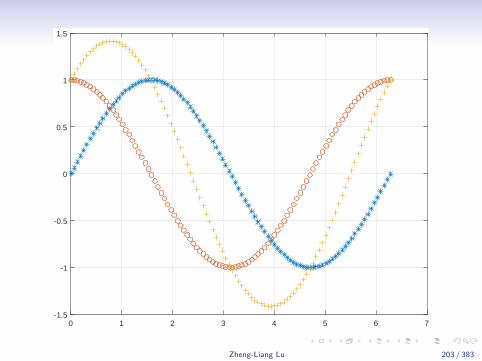
Example 2: Multiple Curves
1 clear; clc;2 x = linspace(0, 2 * pi, 100);3 figure(2); % create Figure 24 plot(x, sin(x), '*', x, cos(x), 'o', x, sin(x) + ...
cos(x), '+');5 grid on;
� Let A be an m-by-n matrix and x be an array of size n.
� Then plot(x ,A) draws a figure for m lines.
Zheng-Liang Lu 202 / 383
0 1 2 3 4 5 6 7-1.5
-1
-0.5
0
0.5
1
1.5
Zheng-Liang Lu 203 / 383

Annotations
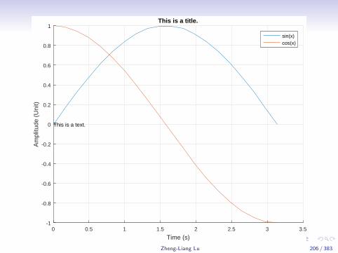
� title(’string’) adds a title to the plot.
� xlabel(’string’) adds a label to the x axis of the plot.
� ylabel(’string’) adds a label to the y axis of the plot.
� legend({’string1’, ’string2’, . . .}) allows you to add a legendfor the multiple lines.
� The legend shows a sample of the line and lists the string youhave specified.
� text(x , y , ’string’) allows you to add a text box for the stringand located at (x , y) in the figure.
Zheng-Liang Lu 204 / 383
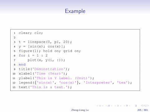
Example
1 clear; clc;2
3 t = linspace(0, pi, 20);4 y = [sin(x); cos(x)];5 figure(1); hold on; grid on;6 for i = 1 : 27 plot(x, y(i, :));8 end9 title('Demonstration');
10 xlabel('Time (Year)');11 ylabel('This is Y label. (Unit)');12 legend({'sin(x)', 'cos(x)'}, 'Interpreter', 'tex');13 text('This is a text.');
Zheng-Liang Lu 205 / 383
0 0.5 1 1.5 2 2.5 3 3.5
Time (s)
-1
-0.8
-0.6
-0.4
-0.2
0
0.2
0.4
0.6
0.8
1
Am
plitu
de (
Uni
t)
This is a title.
This is a text.
sin(x)cos(x)
Zheng-Liang Lu 206 / 383
Exercise: Black-Scholes Model8
� The Black-Scholes model is one of the most famous models infinance engineering.
� Let St be a price process of an underlying asset.
� In this model, the return rate follows a geometric Brownianmotion,
dSt
St= rdt + σdWt ,
where r is the risk-free interest rate, σ is the annualizedvolatility, and dWt is a Wiener process, following the standardnormal distribution.
� We can approximate dS by calculating Si − Si−1 at time i .� This numerical scheme is called finite difference.
8Black and Scholes (1972).Zheng-Liang Lu 207 / 383
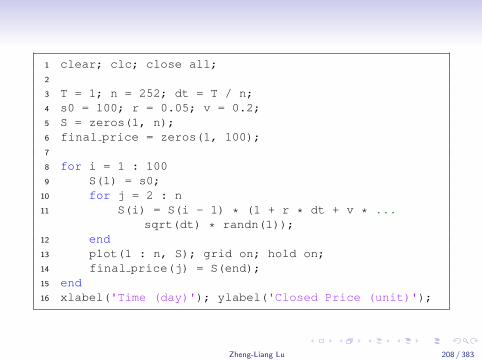
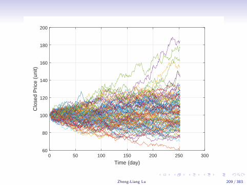
1 clear; clc; close all;2
3 T = 1; n = 252; dt = T / n;4 s0 = 100; r = 0.05; v = 0.2;5 S = zeros(1, n);6 final price = zeros(1, 100);7
8 for i = 1 : 1009 S(1) = s0;
10 for j = 2 : n11 S(i) = S(i - 1) * (1 + r * dt + v * ...
sqrt(dt) * randn(1));12 end13 plot(1 : n, S); grid on; hold on;14 final price(j) = S(end);15 end16 xlabel('Time (day)'); ylabel('Closed Price (unit)');
Zheng-Liang Lu 208 / 383
0 50 100 150 200 250 300
Time (day)
60
80
100
120
140
160
180
200
Clo
sed
Pric
e (u
nit)
Zheng-Liang Lu 209 / 383
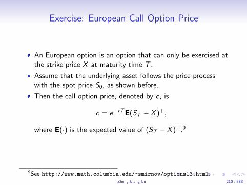
Exercise: European Call Option Price
� An European option is an option that can only be exercised atthe strike price X at maturity time T .
� Assume that the underlying asset follows the price processwith the spot price S0, as shown before.
� Then the call option price, denoted by c , is
c = e−rTE(ST − X )+,
where E(·) is the expected value of (ST − X )+.9
9See http://www.math.columbia.edu/~smirnov/options13.html.Zheng-Liang Lu 210 / 383
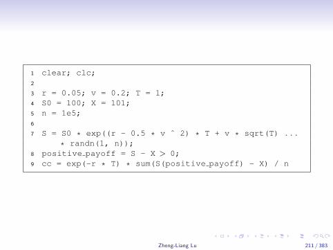
1 clear; clc;2
3 r = 0.05; v = 0.2; T = 1;4 S0 = 100; X = 101;5 n = 1e5;6
7 S = S0 * exp((r - 0.5 * v ˆ 2) * T + v * sqrt(T) ...
* randn(1, n));8 positive payoff = S - X > 0;9 cc = exp(-r * T) * sum(S(positive payoff) - X) / n
Zheng-Liang Lu 211 / 383

Graphics Objects
� Graphics objects are the components for data visualization.
� Each object can be assigned to a unique identifier, called agraphics handle.10
� Through the these handles, you can manipulate theirproperties11 by the following instructions:
� set: set graphics object properties� get: query graphics object properties� reset: reset graphics object properties to their defaults� inspect: open Property Inspector
10Similar to the function handles.11See http:
//www.mathworks.com/help/matlab/graphics-object-properties.html.Zheng-Liang Lu 212 / 383
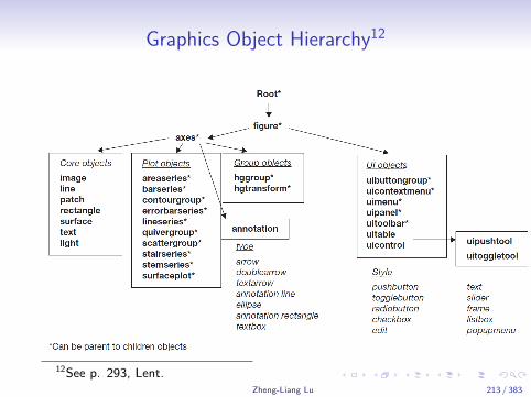
Graphics Object Hierarchy12
12See p. 293, Lent.Zheng-Liang Lu 213 / 383
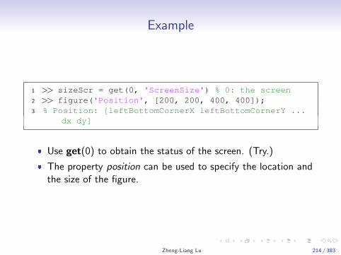
Example
1 >> sizeScr = get(0, 'ScreenSize') % 0: the screen2 >> figure('Position', [200, 200, 400, 400]);3 % Position: [leftBottomCornerX leftBottomCornerY ...
dx dy]
� Use get(0) to obtain the status of the screen. (Try.)
� The property position can be used to specify the location andthe size of the figure.
Zheng-Liang Lu 214 / 383

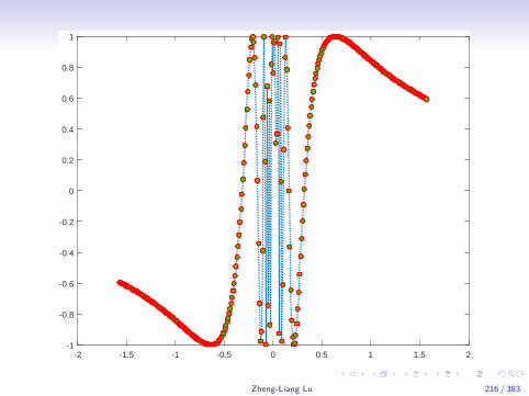
Exercise
1 clear; clc;2
3 x = -0.5 * pi : 0.01 : 0.5 * pi;4 h = plot(x, sin(1 ./ x)); % h is a graphics handle5 set(h, 'marker', 'o');6 set(h, 'markerSize', 5);7 set(h, 'lineWidth', 1.5);8 set(h, 'lineStyle', ':');9 set(h, 'markerEdgeColor', 'r');
10 set(h, 'markerFaceColor', 'g');
� You can use the plot tool in the figures to change theproperties.
Zheng-Liang Lu 215 / 383
-2 -1.5 -1 -0.5 0 0.5 1 1.5 2-1
-0.8
-0.6
-0.4
-0.2
0
0.2
0.4
0.6
0.8
1
Zheng-Liang Lu 216 / 383

Graphics Object Identification13
� The current figure, denoted by gcf, is the window designatedto receive graphics output.
� The current axes, denoted by gca, are the targets forcommands that create axes children.
� The current object, denoted by gco, is the graphics objectcreated or clicked on by the mouse.
13See http://www.mathworks.com/help/matlab/creating_plots/
accessing-object-handles.html.Zheng-Liang Lu 217 / 383
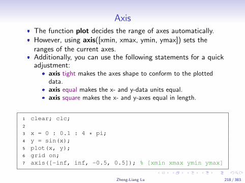
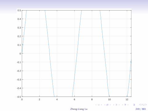
Axis� The function plot decides the range of axes automatically.� However, using axis([xmin, xmax, ymin, ymax]) sets the
ranges of the current axes.� Additionally, you can use the following statements for a quick
adjustment:� axis tight makes the axes shape to conform to the plotted
data.� axis equal makes the x- and y-data units equal.� axis square makes the x- and y-axes equal in length.
1 clear; clc;2
3 x = 0 : 0.1 : 4 * pi;4 y = sin(x);5 plot(x, y);6 grid on;7 axis([-inf, inf, -0.5, 0.5]); % [xmin xmax ymin ymax]
Zheng-Liang Lu 218 / 383
0 2 4 6 8 10 12-0.5
-0.4
-0.3
-0.2
-0.1
0
0.1
0.2
0.3
0.4
0.5
Zheng-Liang Lu 219 / 383

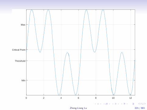
Ticks
� One can change the location of the tick marks on the plot bysetting xtick and ytick of the axes.
1 clear; clc;2
3 x = 0 : 0.1 : 4 * pi;4 plot(x, sin(x) + sin(3 * x));5 axis tight;6 set(gca, 'ytick', [-1 -0.3 0.1 1]);7 set(gca, 'yticklabel', {'Min', 'Threshold', ...
'Critical Point', 'Max'});8 grid on;
� Try ’xtick’ and ’xticklabel’.
Zheng-Liang Lu 220 / 383
0 2 4 6 8 10 12
Min
Threshold
Critical Point
Max
Zheng-Liang Lu 221 / 383

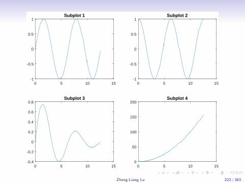
subplot� Multiple plots can be placed in the same figure.� The function subplot(m, n, p) divides the current figure into
an m-by-n grid and uses p to specify the certain subplot.� For example,
1 clear; clc;2
3 x = 0 : 0.1 : 4 * pi;4 subplot(2, 2, 1); plot(x, sin(x)); title('Subplot ...
1');5 subplot(2, 2, 2); plot(x, cos(x)); title('Subplot ...
2');6 subplot(2, 2, 3); plot(x, sin(x) .* exp(-x / 5));7 title('Subplot 3');8 subplot(2, 2, 4); plot(x, x .ˆ 2); title('Subplot ...
4');9 grid on;
Zheng-Liang Lu 222 / 383
0 5 10 15-1
-0.5
0
0.5
1Subplot 1
0 5 10 15-1
-0.5
0
0.5
1Subplot 2
0 5 10 15-0.4
-0.2
0
0.2
0.4
0.6
0.8Subplot 3
0 5 10 150
50
100
150
200Subplot 4
Zheng-Liang Lu 223 / 383

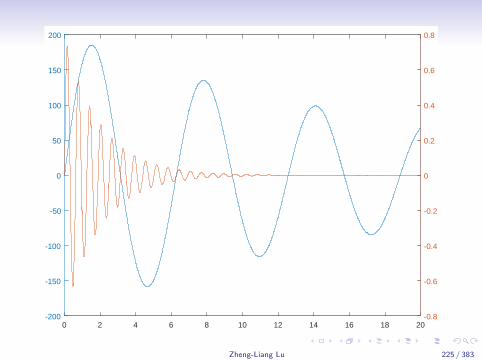
plotyy
� The function plotyy(x1, y1, x2, y2) plots x1 versus y1 withy -axis labeling on the left and plots x2 versus y2 with y -axislabeling on the right.
� For example,
1 clear; clc;2
3 x = 0 : 0.01 : 20;4 y1 = 200 * exp(-0.05 * x) .* sin(x);5 y2 = 0.8 * exp(-0.5 * x) .* sin(10 * x);6 plotyy(x, y1, x, y2);
Zheng-Liang Lu 224 / 383
0 2 4 6 8 10 12 14 16 18 20-200
-150
-100
-50
0
50
100
150
200
-0.8
-0.6
-0.4
-0.2
0
0.2
0.4
0.6
0.8
Zheng-Liang Lu 225 / 383
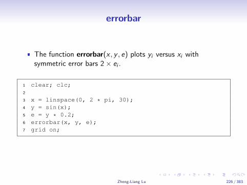
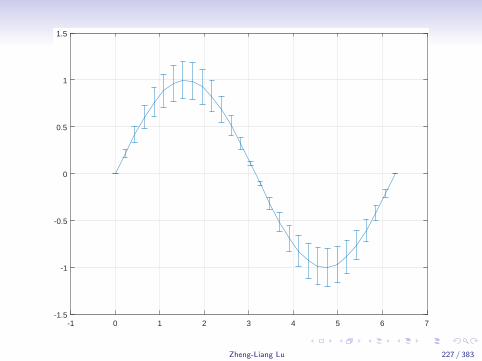
errorbar
� The function errorbar(x , y , e) plots yi versus xi withsymmetric error bars 2× ei .
1 clear; clc;2
3 x = linspace(0, 2 * pi, 30);4 y = sin(x);5 e = y * 0.2;6 errorbar(x, y, e);7 grid on;
Zheng-Liang Lu 226 / 383
-1 0 1 2 3 4 5 6 7-1.5
-1
-0.5
0
0.5
1
1.5
Zheng-Liang Lu 227 / 383
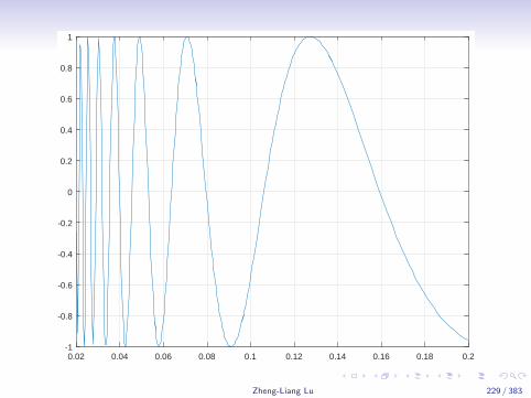
fplot
� The function fplot(func, range) makes a plot for the functionover the range with adaptive steps.
1 clear; clc;2
3 fplot(@(x) sin(1 / x), [0.02 0.2]); grid on;
� Try ezplot.
Zheng-Liang Lu 228 / 383
0.02 0.04 0.06 0.08 0.1 0.12 0.14 0.16 0.18 0.2-1
-0.8
-0.6
-0.4
-0.2
0
0.2
0.4
0.6
0.8
1
Zheng-Liang Lu 229 / 383
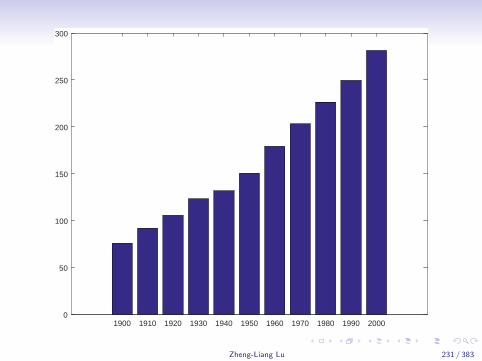
bar14
� The function bar(x , y) draws the bar chart for each column iny at locations specified in x .
� For example,
1 clear; clc;2 x = 1900 : 10 : 2000;3 y = [75.995, 91.972, 105.711, 123.203, 131.669,...4 150.697, 179.323, 203.212, 226.505, 249.633, ...
281.422];5 bar(x, y);
14See http://www.mathworks.com/help/matlab/ref/bar.html.Zheng-Liang Lu 230 / 383
1900 1910 1920 1930 1940 1950 1960 1970 1980 1990 20000
50
100
150
200
250
300
Zheng-Liang Lu 231 / 383
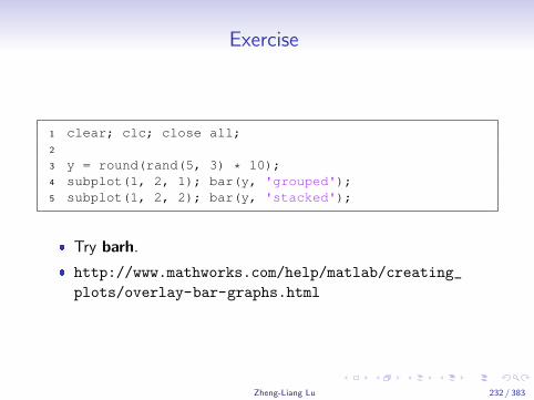
Exercise
1 clear; clc; close all;2
3 y = round(rand(5, 3) * 10);4 subplot(1, 2, 1); bar(y, 'grouped');5 subplot(1, 2, 2); bar(y, 'stacked');
� Try barh.
� http://www.mathworks.com/help/matlab/creating_
plots/overlay-bar-graphs.html
Zheng-Liang Lu 232 / 383

1 2 3 4 50
1
2
3
4
5
6
7
8
9
1 2 3 4 50
2
4
6
8
10
12
14
16
18
20
Zheng-Liang Lu 233 / 383
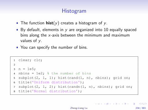
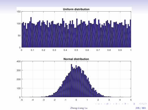
Histogram
� The function hist(y) creates a histogram of y .
� By default, elements in y are organized into 10 equally spacedbins along the x-axis between the minimum and maximumvalues of y .
� You can specify the number of bins.
1 clear; clc;2
3 n = 1e5;4 nbins = 1e2; % the number of bins5 subplot(2, 1, 1); hist(rand(1, n), nbins); grid on;6 title('Uniform distribution');7 subplot(2, 1, 2); hist(randn(1, n), nbins); grid on;8 title('Normal distribution');
Zheng-Liang Lu 234 / 383
0 0.1 0.2 0.3 0.4 0.5 0.6 0.7 0.8 0.9 1
0
50
100
150
Uniform distribution
-5 -4 -3 -2 -1 0 1 2 3 4 5
0
100
200
300
400
Normal distribution
Zheng-Liang Lu 235 / 383
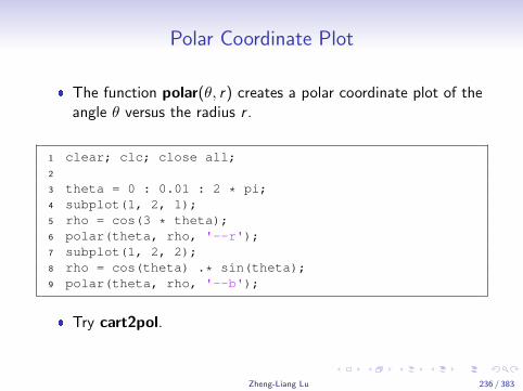
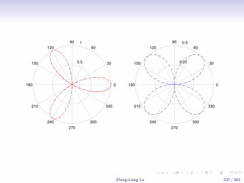
Polar Coordinate Plot
� The function polar(θ, r) creates a polar coordinate plot of theangle θ versus the radius r .
1 clear; clc; close all;2
3 theta = 0 : 0.01 : 2 * pi;4 subplot(1, 2, 1);5 rho = cos(3 * theta);6 polar(theta, rho, '--r');7 subplot(1, 2, 2);8 rho = cos(theta) .* sin(theta);9 polar(theta, rho, '--b');
� Try cart2pol.
Zheng-Liang Lu 236 / 383
0.5
1
30
210
60
240
90
270
120
300
150
330
180 0
0.25
0.5
30
210
60
240
90
270
120
300
150
330
180 0
Zheng-Liang Lu 237 / 383
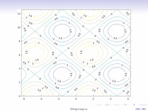
Contours15
� A contour plot displays isolines of Z by calling contour(X , Y ,Z ).
� Instead of using nested loops, you may use the functionmeshgrid which transforms the domain specified by vectors xand y into matrices X and Y .
� Then X and Y can be used for the evaluation of functions off (X ,Y ) by vectorization.
1 clear; clc; close all;2
3 x = linspace(-2 * pi, 2 * pi);4 y = linspace(0, 4 * pi);5 [X, Y] = meshgrid(x, y);6 Z = sin(X) + cos(Y);7 figure; contour(X, Y, Z, 'showtext', 'on');
15You may try contourf.Zheng-Liang Lu 238 / 383
-1.5
-1.5
-1.5
-1.5
-1.5
-1.5
-1.5
-1.5
-1
-1
-1
-1
-1
-1
-1
-1
-0.5
-0.5
-0.5
-0.5
-0.5
-0.5
-0.5
-0.5
-0.5
-0.5
-0.5
0
0
0
0
0
0
0
0
0
0
0
0
0
0
0
0
0.5
0.50.5
0.5
0.5
0.5
0.5
0.5
0.5
0.5
0.5
0.5
0.5
0.5
0.5
1 1
1 1
1
1
11
1
1
1.5 1.5
1.5 1.5
1.5
1.5
1.5
1.5
-6 -4 -2 0 2 4 60
2
4
6
8
10
12
Zheng-Liang Lu 239 / 383
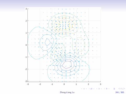
Quiver (Velocity) Plot
� The function quiver(x , y , u, v) plots an arrow (u, v) at thecoordinate (x , y).
1 clear; clc; close all;2 23 [x, y, z] = peaks(20);4 [u, v] = gradient(z);5 figure; hold on; grid on;6 contour(x, y, z, 10);7 quiver(x, y, u, v);8 axis image;
Zheng-Liang Lu 240 / 383
-3 -2 -1 0 1 2 3
-3
-2
-1
0
1
2
3
Zheng-Liang Lu 241 / 383
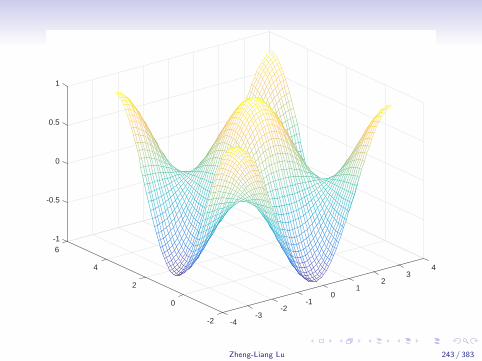
Mesh Plot
� The function mesh(X ,Y ,Z ) draws a wireframe mesh withthe color proportional to surface height, determined by Z .
1 clear; clc; close all;2
3 x = -pi : 0.1 : pi;4 y = x + pi / 2;5 z = zeros(length(x), length(y));6 for i = 1 : length(x)7 for j = 1 : length(y)8 z(i, j) = cos(x(i)) * sin(y(j));9 end
10 end11 figure; mesh(x, y, z');
Zheng-Liang Lu 242 / 383
-16
-0.5
4 4
0
32
0.5
2 10
1
-10-2
-3-2 -4
Zheng-Liang Lu 243 / 383
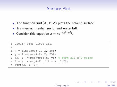
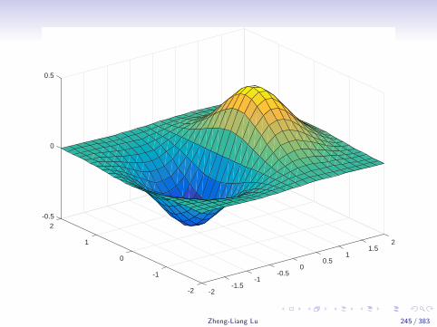
Surface Plot
� The function surf(X ,Y ,Z ) plots the colored surface.
� Try meshz, meshc, surfc, and waterfall.
� Consider this equation z = xe−(x2+y2).
1 clear; clc; close all;2
3 x = linspace(-2, 2, 25);4 y = linspace(-2, 2, 25);5 [X, Y] = meshgrid(x, y); % form all x-y pairs6 Z = X .* exp(-X .ˆ 2 - Y .ˆ 2);7 surf(X, Y, Z);
Zheng-Liang Lu 244 / 383
-0.52
1 2
0
1.510 0.5
0
0.5
-0.5-1-1
-1.5-2 -2
Zheng-Liang Lu 245 / 383
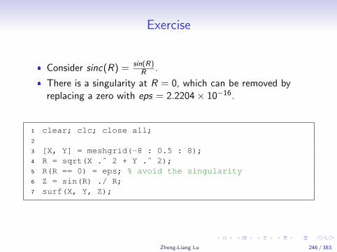
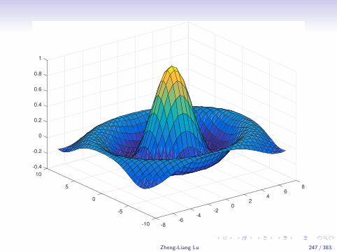
Exercise
� Consider sinc(R) = sin(R)R .
� There is a singularity at R = 0, which can be removed byreplacing a zero with eps = 2.2204× 10⁻¹⁶.
1 clear; clc; close all;2
3 [X, Y] = meshgrid(-8 : 0.5 : 8);4 R = sqrt(X .ˆ 2 + Y .ˆ 2);5 R(R == 0) = eps; % avoid the singularity6 Z = sin(R) ./ R;7 surf(X, Y, Z);
Zheng-Liang Lu 246 / 383
-0.4
10
-0.2
0
0.2
5 8
0.4
6
0.6
40 2
0.8
0
1
-2-5-4
-6-10 -8
Zheng-Liang Lu 247 / 383
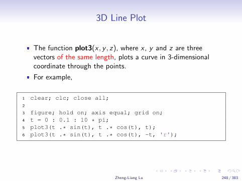
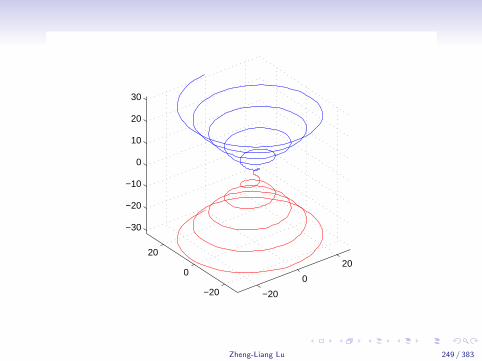
3D Line Plot
� The function plot3(x , y , z), where x , y and z are threevectors of the same length, plots a curve in 3-dimensionalcoordinate through the points.
� For example,
1 clear; clc; close all;2
3 figure; hold on; axis equal; grid on;4 t = 0 : 0.1 : 10 * pi;5 plot3(t .* sin(t), t .* cos(t), t);6 plot3(t .* sin(t), t .* cos(t), -t, 'r');
Zheng-Liang Lu 248 / 383
−20
0
20
−20
0
20
−30
−20
−10
0
10
20
30
Zheng-Liang Lu 249 / 383
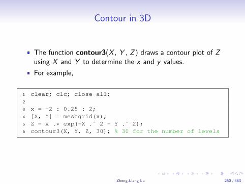
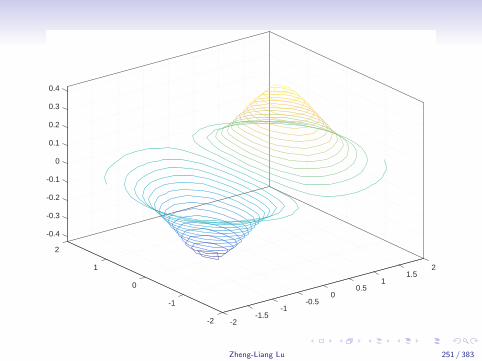
Contour in 3D
� The function contour3(X , Y , Z ) draws a contour plot of Zusing X and Y to determine the x and y values.
� For example,
1 clear; clc; close all;2
3 x = -2 : 0.25 : 2;4 [X, Y] = meshgrid(x);5 Z = X .* exp(-X .ˆ 2 - Y .ˆ 2);6 contour3(X, Y, Z, 30); % 30 for the number of levels
Zheng-Liang Lu 250 / 383
-0.4
2
-0.3
-0.2
-0.1
1 2
0
1.5
0.1
1
0.2
0 0.5
0.3
0.4
0-0.5-1
-1-1.5
-2 -2
Zheng-Liang Lu 251 / 383
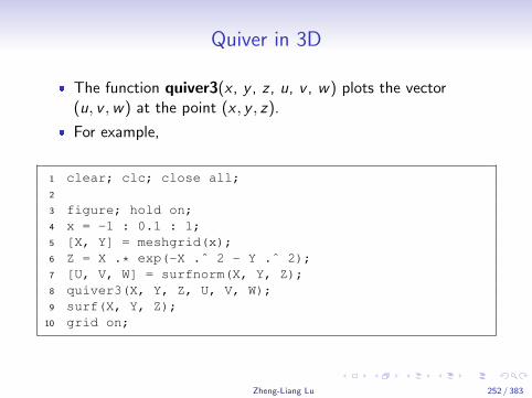
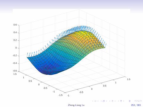
Quiver in 3D
� The function quiver3(x , y , z , u, v , w) plots the vector(u, v ,w) at the point (x , y , z).
� For example,
1 clear; clc; close all;2
3 figure; hold on;4 x = -1 : 0.1 : 1;5 [X, Y] = meshgrid(x);6 Z = X .* exp(-X .ˆ 2 - Y .ˆ 2);7 [U, V, W] = surfnorm(X, Y, Z);8 quiver3(X, Y, Z, U, V, W);9 surf(X, Y, Z);
10 grid on;
Zheng-Liang Lu 252 / 383
-0.61.5
-0.4
-0.2
11.5
0
0.51
0.2
0
0.4
0.5
0.6
-0.5 0-1 -0.5
-1.5 -1
Zheng-Liang Lu 253 / 383
More 3D Plots16
� Try pie3, stem3, fill3, polar3, bar3, ezmesh, and ezsurf.
16See http:
//www.mathworks.com/help/matlab/surface-and-mesh-plots-1.html.Zheng-Liang Lu 254 / 383
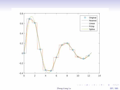
Interpolation18
� Interpolation is a method of constructing new data pointswithin the range of a discrete set of known data points.
� The function interp1(x , v , xq) returns interpolated values ofa 1D function at specific query points.17
� Optional parameters: nearest, linear, spline, pchip, and extrap.� Note that x must be in ascending order.
� Try interp2, interp3, interpn, and interpft.
17See http://www.mathworks.com/help/matlab/ref/interp1.htm.18See https://en.wikipedia.org/wiki/Interpolation.
Zheng-Liang Lu 255 / 383
Example
1 clear; clc; close all;2
3 x = 0 : 4 * pi;4 y = sin(x) .* exp(-x / 5);5 xi = 0 : 0.1 : 4 * pi;6 y1 = interp1(x, y, xi, 'nearest');7 y2 = interp1(x, y, xi, 'linear');8 y3 = interp1(x, y, xi, 'pchip');9 y4 = interp1(x, y, xi, 'spline');
10 plot(x, y, 'o', xi, y1, xi, y2, xi, y3, xi, y4);11 legend('Original', 'Nearest', 'Linear', 'Pchip', ...
'Spline');
Zheng-Liang Lu 256 / 383
0 2 4 6 8 10 12 14-0.4
-0.2
0
0.2
0.4
0.6
0.8
OriginalNearestLinearPchipSpline
Zheng-Liang Lu 257 / 383
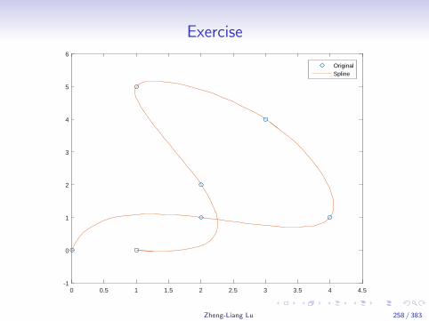
Exercise
0 0.5 1 1.5 2 2.5 3 3.5 4 4.5-1
0
1
2
3
4
5
6
OriginalSpline
Zheng-Liang Lu 258 / 383
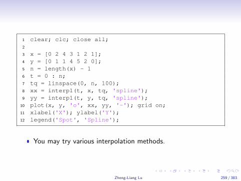
1 clear; clc; close all;2
3 x = [0 2 4 3 1 2 1];4 y = [0 1 1 4 5 2 0];5 n = length(x) - 16 t = 0 : n;7 tq = linspace(0, n, 100);8 xx = interp1(t, x, tq, 'spline');9 yy = interp1(t, y, tq, 'spline');
10 plot(x, y, 'o', xx, yy, '-'); grid on;11 xlabel('X'); ylabel('Y');12 legend('Spot', 'Spline');
� You may try various interpolation methods.
Zheng-Liang Lu 259 / 383
Surface Reconstruction
� In practice, we collect the data from experiments.
� One posterior analysis on these data points is to find thepossible curves or surfaces to fit the observed data points.
� Let (x , y , z) be the data points.
� Then the function zq = griddata(x , y , z , xq, yq) interpolatesthe data points for the region specified by (xq, yq) toreconstructs the surface.
Zheng-Liang Lu 260 / 383
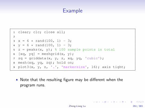
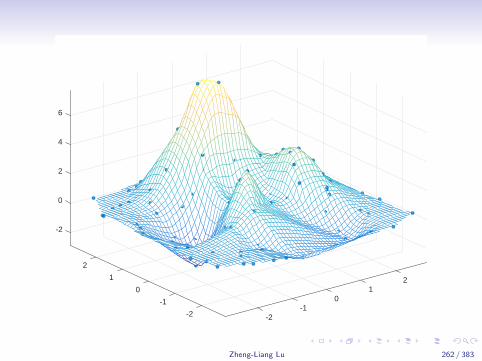
Example
1 clear; clc; close all;2
3 x = 6 * rand(100, 1) - 3;4 y = 6 * rand(100, 1) - 3;5 z = peaks(x, y); % 100 sample points in total6 [xq, yq] = meshgrid(x, y);7 zq = griddata(x, y, z, xq, yq, 'cubic');8 mesh(xq, yq, zq); hold on;9 plot3(x, y, z, '.', 'markersize', 16); axis tight;
� Note that the resulting figure may be different when theprogram runs.
Zheng-Liang Lu 261 / 383
-2
0
2
2
1 2
4
10
6
0-1-1
-2 -2
Zheng-Liang Lu 262 / 383
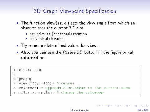
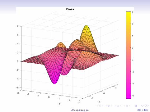
3D Graph Viewpoint Specification
� The function view(az, el) sets the view angle from which anobserver sees the current 3D plot.
� az: azimuth (horizontal) rotation� el: vertical elevation
� Try some predetermined values for view.
� Also, you can use the Rotate 3D button in the figure or callrotate3d on.
1 clear; clc;2
3 peaks;4 view([60, -15]); % degree5 colorbar; % appends a colorbar to the current axes6 colormap spring; % change the colormap
Zheng-Liang Lu 263 / 383
32
1 -20
y
8
-1
6
4
-2
2
0
0
x
-2
-3
-4
-6
Peaks
2
-6
-4
-2
0
2
4
6
8
Zheng-Liang Lu 264 / 383
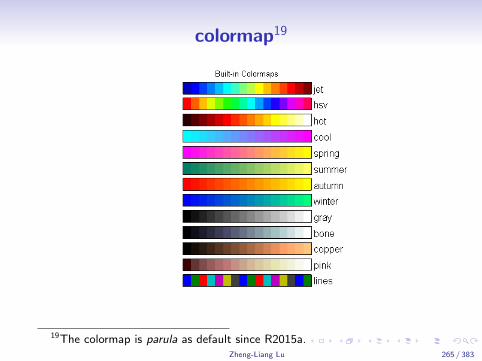
colormap19
19The colormap is parula as default since R2015a.Zheng-Liang Lu 265 / 383
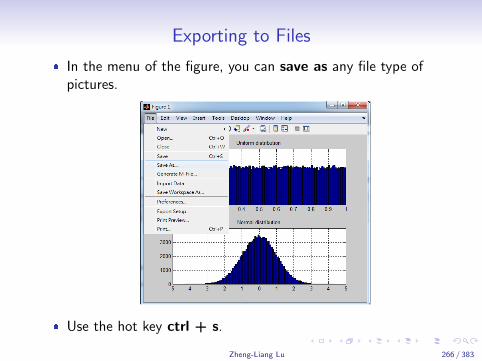
Exporting to Files
� In the menu of the figure, you can save as any file type ofpictures.
� Use the hot key ctrl + s.
Zheng-Liang Lu 266 / 383

� The function print(gh, ’-type’, ’fileName’) saves the contentsof the current figure, herein gh, with a specified file type anda file name.
� For example,
1 clear; clc;2
3 surf(peaks);4 print(gcf, '-djpeg', 'peaks.jpg');
� You can find more optional arguments here.
Zheng-Liang Lu 267 / 383
1 >> Lecture 52 >>3 >> -- User-Controlled Input and Output4 >>
Zheng-Liang Lu 268 / 383
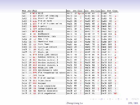
American Standard Code for Information Interchange(ASCII)21
� Everything in the computer is encoded in binary.
� ASCII codes represent text in computers, communicationsequipment, and other devices that use text.
� ASCII is a character-encoding scheme originally based on theEnglish alphabet that encodes 128 specified characters intothe 7-bit binary integers (see the next page).
� Unicode20 became a standard for the modern systems from2007.
� Unicode includes ASCII.
20See Unicode 8.0 Character Code Charts.21The first version was in 1967. See ASCII.
Zheng-Liang Lu 269 / 383
Zheng-Liang Lu 270 / 383

Import Tool
� One can load data from the specified file byimportdata(filename), which can recognize the common fileextensions.
� For example, txt, csv, jpg, bmp, wav, avi, and xls.22
� Note that the file name must be a string.� If not, importdata interprets the file as a delimited ASCII file
as default.� importdata(’-pastespecial’) loads data from the system
clipboard rather than from a file.
� Try uiimport.
22See http://www.mathworks.com/help/matlab/import_export/
supported-file-formats.html.Zheng-Liang Lu 271 / 383
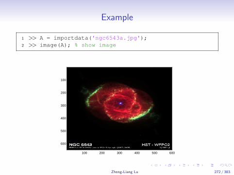
Example
1 >> A = importdata('ngc6543a.jpg');2 >> image(A); % show image
100 200 300 400 500 600
100
200
300
400
500
600
Zheng-Liang Lu 272 / 383
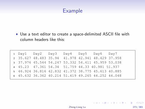
Example
� Use a text editor to create a space-delimited ASCII file withcolumn headers like this:
1 Day1 Day2 Day3 Day4 Day5 Day6 Day72 35.627 48.483 35.94 41.978 42.941 48.429 37.9583 37.976 45.544 54.247 53.332 54.411 45.959 53.0384 45.23 47.361 54.34 51.759 44.33 40.981 51.9375 46.924 36.816 42.832 41.372 38.775 45.613 40.8856 45.632 36.362 40.214 51.419 49.265 44.252 44.048
Zheng-Liang Lu 273 / 383
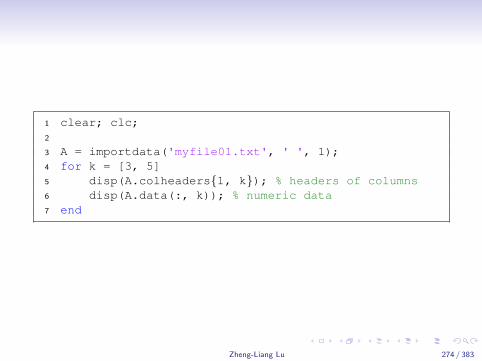
1 clear; clc;2
3 A = importdata('myfile01.txt', ' ', 1);4 for k = [3, 5]5 disp(A.colheaders{1, k}); % headers of columns6 disp(A.data(:, k)); % numeric data7 end
Zheng-Liang Lu 274 / 383
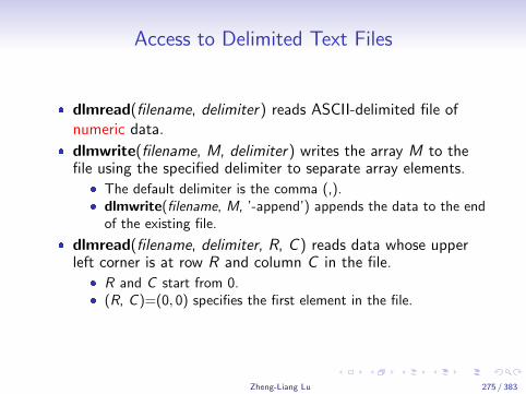
Access to Delimited Text Files
� dlmread(filename, delimiter) reads ASCII-delimited file ofnumeric data.
� dlmwrite(filename, M, delimiter) writes the array M to thefile using the specified delimiter to separate array elements.
� The default delimiter is the comma (,).� dlmwrite(filename, M, ’-append’) appends the data to the end
of the existing file.
� dlmread(filename, delimiter, R, C ) reads data whose upperleft corner is at row R and column C in the file.
� R and C start from 0.� (R, C )=(0, 0) specifies the first element in the file.
Zheng-Liang Lu 275 / 383

Example
� Write to the file.
1 >> M = gallery('integerdata', 100, [5 8], 0);2 >> dlmwrite('myfile.txt', M, 'delimiter', '\t');
� Read from the file.
1 >> dlmread('myfile.txt', '\t')2 >> dlmread('myfile.txt', '\t', 2, 3)
Zheng-Liang Lu 276 / 383

textread
� The function textread23 is useful for reading text files withknown formats.
� For example,
[A,B,C , . . .] = textread(filename, formatter)
reads data from the file filename into the variables A, B,C,. . . by using the specified format formatter, whichdetermines the number and types of arguments.
� The formatter is used as templates for data.
� We often use conversion specifiers to render the arguments inplace of certain placeholders (see the next page).
23You may try textscan in newer versions.Zheng-Liang Lu 277 / 383
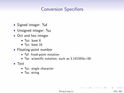
Conversion Specifiers
� Signed integer: %d
� Unsigned integer: %u
� Oct and hex integer� %o: base 8� %x: base 16
� Floating-point number� %f: fixed-point notation� %e: scientific notation, such as 3.141593e+00
� Text� %c: single character� %s: string
Zheng-Liang Lu 278 / 383
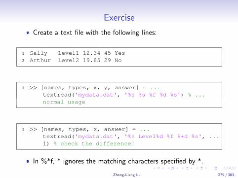
Exercise
� Create a text file with the following lines:
1 Sally Level1 12.34 45 Yes2 Arthur Level2 19.85 29 No
1 >> [names, types, x, y, answer] = ...textread('mydata.dat', '%s %s %f %d %s') % ...normal usage
1 >> [names, types, x, answer] = ...textread('mydata.dat', '%s Level%d %f %*d %s', ...1) % check the difference!
� In %*f, * ignores the matching characters specified by *.
Zheng-Liang Lu 279 / 383
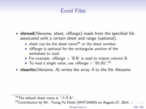
Excel Files
� xlsread(filename, sheet, xlRange) reads from the specified fileassoicated with a certain sheet and range (optional).
� sheet can be the sheet name24 or the sheet number.� xlRange is optional for the rectangular portion of the
worksheet to read.� For example, xlRange = ’B:B’ is used to import column B.� To read a single value, use xlRange = ’B1:B1’.25
� xlswrite(filename, A) writes the array A to the file filename.
24The default sheet name is “工作表”.25Contribution by Mr. Tsung-Yu Hsieh (MAT24409) on August 27, 2014.
Zheng-Liang Lu 280 / 383
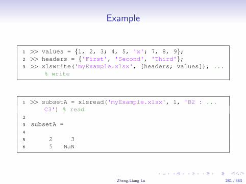
Example
1 >> values = {1, 2, 3; 4, 5, 'x'; 7, 8, 9};2 >> headers = {'First', 'Second', 'Third'};3 >> xlswrite('myExample.xlsx', [headers; values]); ...
% write
1 >> subsetA = xlsread('myExample.xlsx', 1, 'B2 : ...C3') % read
2
3 subsetA =4
5 2 36 5 NaN
Zheng-Liang Lu 281 / 383
Low-Level File I/O
� When the high-level functions cannot import your data, youmay consider to use low-level file I/O.
� Low-level file I/O functions allow the most control overreading/writing data to files.
� The normal procedure is as follows:
1. Open a file.2. Read/write data into the file.3. Close the file.
Zheng-Liang Lu 282 / 383
Open Files
� fopen(filename, permission) is used to deal with a file, where� filename refers to the filename, and� permission specifies the file access code: ’r’, ’w’, ’a’.
� Note that the permission code ’w’ is used to write the file byoverwriting the previous result.
� If you want to add new result to an existed file, use permissioncode ’r’.
� This function returns an integer (at least 3) as the fileidentifier assigned to the file handle.26
� If the return number is −1, then fopen fails to open this filewith ’r’.
26Matlab reserves 1 and 2 for the standard output and the standard error,respectively.
Zheng-Liang Lu 283 / 383
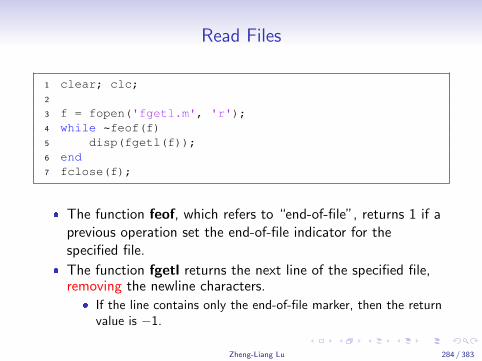
Read Files
1 clear; clc;2
3 f = fopen('fgetl.m', 'r');4 while ~feof(f)5 disp(fgetl(f));6 end7 fclose(f);
� The function feof, which refers to “end-of-file”, returns 1 if aprevious operation set the end-of-file indicator for thespecified file.
� The function fgetl returns the next line of the specified file,removing the newline characters.
� If the line contains only the end-of-file marker, then the returnvalue is −1.
Zheng-Liang Lu 284 / 383

Close Files
� fclose(f ) closes the opened file referenced by f .
� fclose(’all’) closes all opened files.
� fclose returns a status of 0 when the close operation issuccessful.
� Otherwise, it returns −1.
Zheng-Liang Lu 285 / 383
Exercise
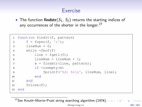
� The function findstr(S1, S2) returns the starting indices ofany occurrences of the shorter in the longer.27
1 function findit(f, pattern)2 f = fopen(f, 'r');3 lineNum = 0;4 while ~feof(f)5 line = fgetl(f);6 lineNum = lineNum + 1;7 w = findstr(line, pattern);8 if ~isempty(w)9 fprintf('%d: %s\n', lineNum, line);
10 end11 end12 fclose(f);13 end
27See Knuth–Morris–Pratt string searching algorithm (1974).Zheng-Liang Lu 286 / 383
Write Files
� Recall that fprintf(format, A1, . . . ,An) displays the results onthe screen according to the preset format.
� format: a format for the output fields; it should be a string.� A1, . . . ,An: arrays for each output field.
� In fact, fprintf(f, format, A1, . . . ,An) applies the format to allelements of arrays A1, . . . ,An in column order, and writes to atext file referenced by the file handle f.
Zheng-Liang Lu 287 / 383
Example
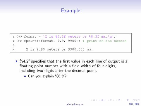
1 >> format = 'X is %4.2f meters or %8.3f mm.\n';2 >> fprintf(format, 9.9, 9900); % print on the screen3
4 X is 9.90 meters or 9900.000 mm.
� %4.2f specifies that the first value in each line of output is afloating-point number with a field width of four digits,including two digits after the decimal point.
� Can you explain %8.3f?
Zheng-Liang Lu 288 / 383
Exercise
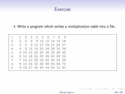
� Write a program which writes a multiplication table into a file.
1 1 2 3 4 5 6 7 8 92 2 4 6 8 10 12 14 16 183 3 6 9 12 15 18 21 24 274 4 8 12 16 20 24 28 32 365 5 10 15 20 25 30 35 40 456 6 12 18 24 30 36 42 48 547 7 14 21 28 35 42 49 56 638 8 16 24 32 40 48 56 64 729 9 18 27 36 45 54 63 72 81
Zheng-Liang Lu 289 / 383
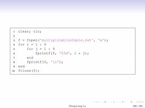
1 clear; clc;2
3 f = fopen('multiplicationTable.txt', 'w');4 for i = 1 : 95 for j = 1 : 96 fprintf(f, '%3d', i * j);7 end8 fprintf(f, '\n');9 end
10 fclose(f);
Zheng-Liang Lu 290 / 383
1 >> Lecture 62 >>3 >> -- Strings and Regular Expressions4 >>
Zheng-Liang Lu 291 / 383
Characters and Strings (Revisited)
� A character array is a sequence of characters, just as anumeric array is a sequence of numbers.
� A string array is a container for pieces of text, providing a setof functions for working with text as data.
� Cell arrays can be used to contain couples of strings.
Zheng-Liang Lu 292 / 383
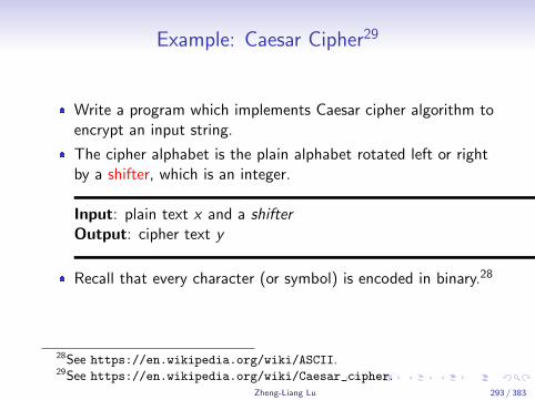
Example: Caesar Cipher29
� Write a program which implements Caesar cipher algorithm toencrypt an input string.
� The cipher alphabet is the plain alphabet rotated left or rightby a shifter, which is an integer.
Input: plain text x and a shifterOutput: cipher text y
� Recall that every character (or symbol) is encoded in binary.28
28See https://en.wikipedia.org/wiki/ASCII.29See https://en.wikipedia.org/wiki/Caesar_cipher.
Zheng-Liang Lu 293 / 383
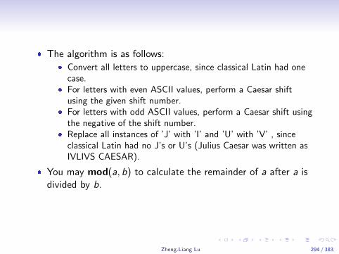
� The algorithm is as follows:� Convert all letters to uppercase, since classical Latin had one
case.� For letters with even ASCII values, perform a Caesar shift
using the given shift number.� For letters with odd ASCII values, perform a Caesar shift using
the negative of the shift number.� Replace all instances of ’J’ with ’I’ and ’U’ with ’V’ , since
classical Latin had no J’s or U’s (Julius Caesar was written asIVLIVS CAESAR).
� You may mod(a, b) to calculate the remainder of a after a isdivided by b.
Zheng-Liang Lu 294 / 383
Introduction
� A regular expression, also called a pattern, is an expressionused to specify a set of strings required for a particularpurpose.30
� Usually this pattern is widely used by string searchingalgorithms for ”find” or ”find and replace” operations onstrings.
30See https://en.wikipedia.org/wiki/Regular_expression.Zheng-Liang Lu 295 / 383
Example
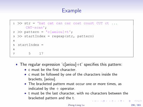
1 >> str = 'bat cat can car coat court CUT ct ...CAT-scan';
2 >> pattern = 'c[aeiou]+t';3 >> startIndex = regexp(str, pattern)4
5 startIndex =6
7 5 17
� The regular expression ’c[aeiou]+t’ specifies this pattern:� c must be the first character.� c must be followed by one of the characters inside the
brackets, [aeiou].� The bracketed pattern must occur one or more times, as
indicated by the + operator.� t must be the last character, with no characters between the
bracketed pattern and the t.
Zheng-Liang Lu 296 / 383

Formalisms
Operator Definition
| Boolean OR
* 0 or more times consecutively
? 0 times or 1 time
+ 1 or more times consecutively
{n} exactly n times consecutively
{m, } at least m times consecutively
{, n} at most n times consecutively
{m, n} at least m times, but no more than n times consecutively
Zheng-Liang Lu 297 / 383
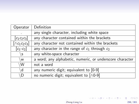
Operator Definition
. any single character, including white space
[c1c2c3] any character contained within the brackets
[∧c1c2c3] any character not contained within the brackets
[c1-c2] any character in the range of c1 through c2\s any white-space character
\w a word; any alphabetic, numeric, or underscore character
\W not a word
\d any numeric digit; equivalent to [0-9]
\D no numeric digit; equivalent to [∧0-9]
Zheng-Liang Lu 298 / 383
Example
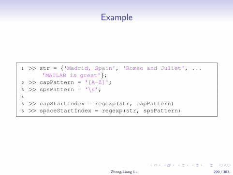
1 >> str = {'Madrid, Spain', 'Romeo and Juliet', ...'MATLAB is great'};
2 >> capPattern = '[A-Z]';3 >> spsPattern = '\s';4
5 >> capStartIndex = regexp(str, capPattern)6 >> spaceStartIndex = regexp(str, spsPattern)
Zheng-Liang Lu 299 / 383

Keywords for Outputs
Output Keyword Returns
’start’ starting indices of all matches, by default
’end’ ending indices of all matches
’match’ text of each substring that matches the pattern
’tokens’ text of each captured token
’split’ text of nonmatching substrings
’names’ name and text of each named token
Zheng-Liang Lu 300 / 383
Example: Match
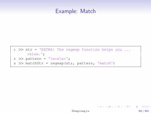
1 >> str = 'EXTRA! The regexp function helps you ...relax.';
2 >> pattern = '\w*x\w*';3 >> matchStr = regexp(str, pattern, 'match')
Zheng-Liang Lu 301 / 383
Example: Split
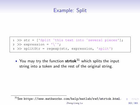
1 >> str = ['Split ˆthis text into ˆseveral pieces'];2 >> expression = '\ˆ';3 >> splitStr = regexp(str, expression, 'split')
� You may try the function strtok31 which splits the inputstring into a token and the rest of the original string.
31See https://www.mathworks.com/help/matlab/ref/strtok.html.Zheng-Liang Lu 302 / 383

Exercise: Web Crawler
� Write a script which collects the names of HTML tags bydefining a token within a regular expression.
� For example,
1 >> str = '<title>My Title</title><p>Here is some ...text.</p>';
2 >> pattern = '<(\w+).*>.*</\1>';3 >> [tokens, matches] = regexp(str, pattern, ...
'tokens', 'match')
Zheng-Liang Lu 303 / 383
Example: Names
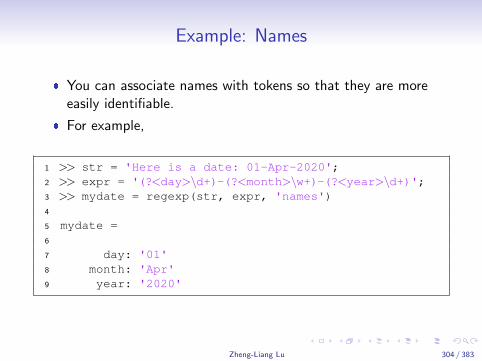
� You can associate names with tokens so that they are moreeasily identifiable.
� For example,
1 >> str = 'Here is a date: 01-Apr-2020';2 >> expr = '(?<day>\d+)-(?<month>\w+)-(?<year>\d+)';3 >> mydate = regexp(str, expr, 'names')4
5 mydate =6
7 day: '01'8 month: 'Apr'9 year: '2020'
Zheng-Liang Lu 304 / 383
More Relevant Functions
� Check contains, regexpi, regexprep, regexptranslate,replace, strfind, strjoin, strrep, and strsplit.
� See the following links:� https:
//www.mathworks.com/help/matlab/ref/regexp.html� https://en.wikipedia.org/wiki/Regular_expression� https://regexone.com/
Zheng-Liang Lu 305 / 383
1 >> Lecture 72 >>3 >> -- Matrix Computation4 >>
Zheng-Liang Lu 306 / 383
Vectors
� Let R be the set of all real numbers.
� Rm×1 denotes the vector space of all m-by-1 column vectors:
u = (ui ) =
u1...
um
. (1)
� Similarly, the row vector v ∈ R1×n is
v = (vi ) =[
v1 · · · vn]. (2)
Zheng-Liang Lu 307 / 383

Matrices
� Rm×n denotes the vector space of all m-by-n real matrices A:
A = (aij) =
a11 · · · a1n...
. . ....
am1 · · · amn
.� Recall that we use the subscripts to reference a particular
element in a matrix.
� The definition for complex matrices is similar.
Zheng-Liang Lu 308 / 383
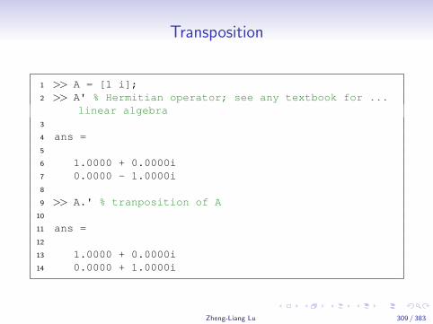
Transposition
1 >> A = [1 i];2 >> A' % Hermitian operator; see any textbook for ...
linear algebra3
4 ans =5
6 1.0000 + 0.0000i7 0.0000 - 1.0000i8
9 >> A.' % tranposition of A10
11 ans =12
13 1.0000 + 0.0000i14 0.0000 + 1.0000i
Zheng-Liang Lu 309 / 383
Arithmetic Operations
� Let aij and bij be the elements of the matrices A andB ∈ Rm×n for 1 ≤ i ≤ m and 1 ≤ j ≤ n.
� Then C = A± B can be calculated by cij = aij ± bij . (Try.)
Zheng-Liang Lu 310 / 383
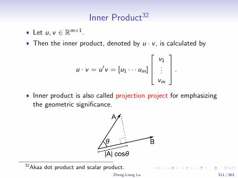
Inner Product32
� Let u, v ∈ Rm×1.
� Then the inner product, denoted by u · v , is calculated by
u · v = u′v = [u1 · · · um]
v1...
vm
.� Inner product is also called projection project for emphasizing
the geometric significance.
32Akaa dot product and scalar product.Zheng-Liang Lu 311 / 383
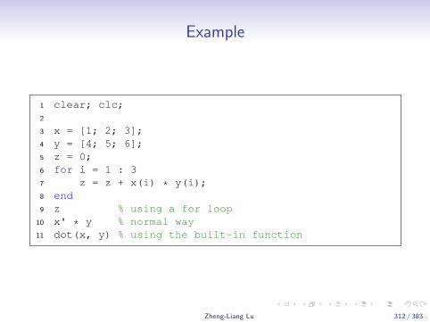
Example
1 clear; clc;2
3 x = [1; 2; 3];4 y = [4; 5; 6];5 z = 0;6 for i = 1 : 37 z = z + x(i) * y(i);8 end9 z % using a for loop
10 x' * y % normal way11 dot(x, y) % using the built-in function
Zheng-Liang Lu 312 / 383
Exercise
� Let u and v be any two vectors in Rm×1.
� Write a program that returns the angle between u and v .
Input: u, vOutput: θ in radian
� You may use norm(u) to calculate the length of u.33
� Alternatively, use subspace(u, v).
33See https://en.wikipedia.org/wiki/Norm_(mathematics).Zheng-Liang Lu 313 / 383
Generalization of Inner Product
� For simplicity, consider x ∈ R.
� Let f (x) be a real-valued function.
� Let g(x) be a basis function.34
� Then we can define the inner product of f and g on [a, b] by
〈f , g〉 =
∫ b
af (x)g(x)dx .
� There exist plenty of basis functions which can be used torepresent the functions.35
34See https://en.wikipedia.org/wiki/Basis_function.35See https://en.wikipedia.org/wiki/Eigenfunction and
https://en.wikipedia.org/wiki/Approximation_theory.Zheng-Liang Lu 314 / 383
� For example, Fourier transform is widely used in engineeringand science.
� Fourier integral36 is defined as
F (ω) =
∫ ∞−∞
f (t)e−iωtdt
where f (t) is a square-integrable function.
� The Fast Fourier transform (FFT) algorithm computes thediscrete Fourier transform (DFT) in O(n log n) time.37,38
36See https://en.wikipedia.org/wiki/Fourier_transform.37Cooley and Tukey (1965).38See https://en.wikipedia.org/wiki/Fast_Fourier_transform.
Zheng-Liang Lu 315 / 383
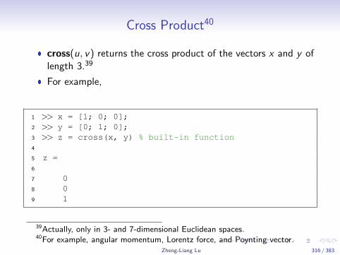
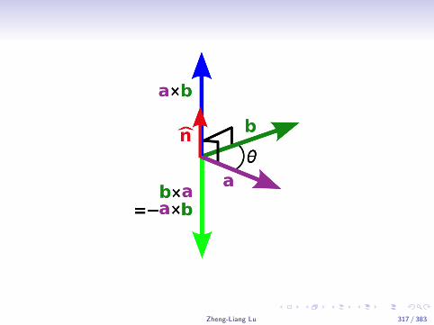
Cross Product40
� cross(u, v) returns the cross product of the vectors x and y oflength 3.39
� For example,
1 >> x = [1; 0; 0];2 >> y = [0; 1; 0];3 >> z = cross(x, y) % built-in function4
5 z =6
7 08 09 1
39Actually, only in 3- and 7-dimensional Euclidean spaces.40For example, angular momentum, Lorentz force, and Poynting vector.
Zheng-Liang Lu 316 / 383
Zheng-Liang Lu 317 / 383
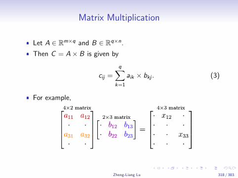
Matrix Multiplication
� Let A ∈ Rm×q and B ∈ Rq×n.
� Then C = A× B is given by
cij =
q∑k=1
aik × bkj . (3)
� For example,
Zheng-Liang Lu 318 / 383
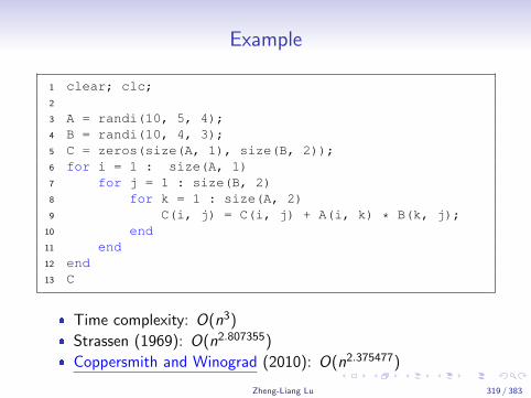
Example
1 clear; clc;2
3 A = randi(10, 5, 4);4 B = randi(10, 4, 3);5 C = zeros(size(A, 1), size(B, 2));6 for i = 1 : size(A, 1)7 for j = 1 : size(B, 2)8 for k = 1 : size(A, 2)9 C(i, j) = C(i, j) + A(i, k) * B(k, j);
10 end11 end12 end13 C
� Time complexity: O(n3)
� Strassen (1969): O(n2.807355)
� Coppersmith and Winograd (2010): O(n2.375477)
Zheng-Liang Lu 319 / 383
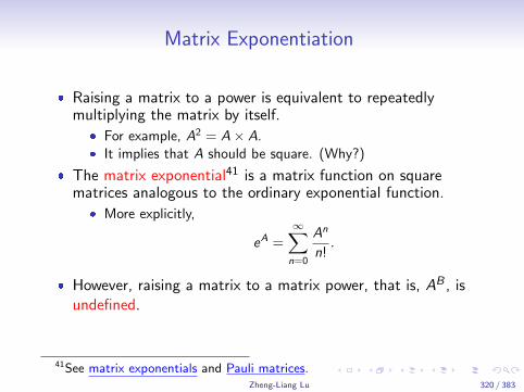
Matrix Exponentiation
� Raising a matrix to a power is equivalent to repeatedlymultiplying the matrix by itself.
� For example, A2 = A× A.� It implies that A should be square. (Why?)
� The matrix exponential41 is a matrix function on squarematrices analogous to the ordinary exponential function.
� More explicitly,
eA =∞∑n=0
An
n!.
� However, raising a matrix to a matrix power, that is, AB , isundefined.
41See matrix exponentials and Pauli matrices.Zheng-Liang Lu 320 / 383
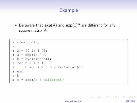
Example
� Be aware that exp(A) and exp(1)A are different for anysquare matrix A.
1 clear; clc;2
3 A = [0 1; 1 0];4 a = exp(1) ˆ A5 b = eye(size(A));6 for n = 1 : 107 b = b + X ˆ n / factorial(n);8 end9 b
10 c = exp(A) % different?
Zheng-Liang Lu 321 / 383
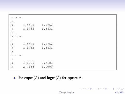
1 a =2
3 1.5431 1.17524 1.1752 1.54315
6 b =7
8 1.5431 1.17529 1.1752 1.5431
10
11 c =12
13 1.0000 2.718314 2.7183 1.0000
� Use expm(A) and logm(A) for square A.
Zheng-Liang Lu 322 / 383
Determinants
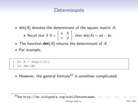
� det(A) denotes the determinant of the square matrix A.
� Recall that if A =
[a bc d
], then det(A) = ad − bc.
� The function det(A) returns the determinant of A.
� For example,
1 >> A = magic(3);2 >> det(A)
� However, the general formula42 is somehow complicated.
42See http://en.wikipedia.org/wiki/Determinant.Zheng-Liang Lu 323 / 383
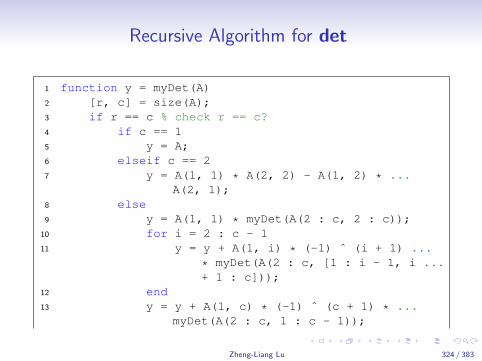
Recursive Algorithm for det
1 function y = myDet(A)2 [r, c] = size(A);3 if r == c % check r == c?4 if c == 15 y = A;6 elseif c == 27 y = A(1, 1) * A(2, 2) - A(1, 2) * ...
A(2, 1);8 else9 y = A(1, 1) * myDet(A(2 : c, 2 : c));
10 for i = 2 : c - 111 y = y + A(1, i) * (-1) ˆ (i + 1) ...
* myDet(A(2 : c, [1 : i - 1, i ...+ 1 : c]));
12 end13 y = y + A(1, c) * (-1) ˆ (c + 1) * ...
myDet(A(2 : c, 1 : c - 1));
Zheng-Liang Lu 324 / 383
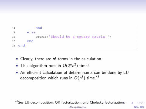
14 end15 else16 error('Should be a square matrix.')17 end18 end
� Clearly, there are n! terms in the calculation.
� This algorithm runs in O(2nn2) time!
� An efficient calculation of determinants can be done by LUdecomposition which runs in O(n3) time.43
43See LU decomposition, QR factorization, and Cholesky factorization.Zheng-Liang Lu 325 / 383
Inverse Matrices
� A ∈ Rn×n is invertible if there exists B ∈ Rn×n such that
A× B = B × A = In,
where In denotes the n-by-n identity matrix.� You can use eye(n) to generate an identity matrix In.
� A is invertible if and only if det(A) 6= 0.
� The function inv(A) returns the inverse of A.
Zheng-Liang Lu 326 / 383
� For example,
1 >> A = pascal(4); % Pascal matrix2 >> B = inv(A)
� However, inv(A) may return a result even if A isill-conditioned.44
� For example,
det
1 2 34 5 67 8 9
= 0.
44Try rcond.Zheng-Liang Lu 327 / 383
First-Order Approximation46
� Let f (x) be a nonlinear function which is infinitelydifferentiable at x0.
� By Taylor’s expansion45, we have
f (x) ≈ f (x0) + f ′(x0)(x − x0) + O(∆x2),
where ∆x2 is the higher-order term, which can be neglectedas ∆x → x0.
� So a nonlinear function can be reduced by its first-orderapproximation.
45See https://en.wikipedia.org/wiki/Taylor_series.46For example, the Newtonian equation is only a low-speed approximation to
Einstein’s total energy, given by E = m0c2√
1−(v/c)2, where m0 is the rest mass and
v is the velocity relative to the inertial coordinate. By applying the first-orderapproximation, E ≈ m0c
2 + 12mv 2.
Zheng-Liang Lu 328 / 383

System of Linear Equations
� A system of linear equations is a set of linear equationsinvolving the same set of variables.
� For example, nodal analysis by Kirchhoff’s Laws.
Zheng-Liang Lu 329 / 383
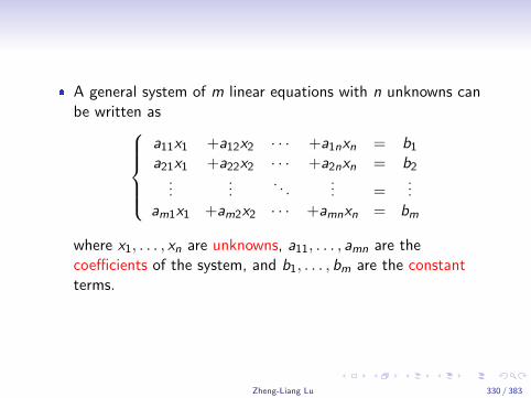
� A general system of m linear equations with n unknowns canbe written as
a11x1 +a12x2 · · · +a1nxn = b1
a21x1 +a22x2 · · · +a2nxn = b2...
.... . .
... =...
am1x1 +am2x2 · · · +amnxn = bm
where x1, . . . , xn are unknowns, a11, . . . , amn are thecoefficients of the system, and b1, . . . , bm are the constantterms.
Zheng-Liang Lu 330 / 383
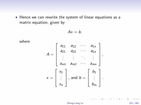
� Hence we can rewrite the system of linear equations as amatrix equation, given by
Ax = b.
where
A =
a11 a12 · · · a1na21 a22 · · · a2n
......
. . ....
am1 am2 · · · amn
,
x =
x1...
xn
, and b =
b1...
bm
.
Zheng-Liang Lu 331 / 383
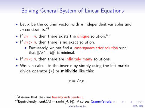
Solving General System of Linear Equations
� Let x be the column vector with n independent variables andm constraints.47
� If m = n, then there exists the unique solution.48
� If m > n, then there is no exact solution.� Fortunately, we can find a least-squares error solution such
that ‖Ax ′ − b‖2 is minimal.
� If m < n, then there are infinitely many solutions.
� We can calculate the inverse by simply using the left matrixdivide operator (\) or mldivide like this:
x = A\b.
47Assume that they are linearly independent.48Equivalently, rank(A) = rank([A, b]). Also see Cramer’s rule.
Zheng-Liang Lu 332 / 383
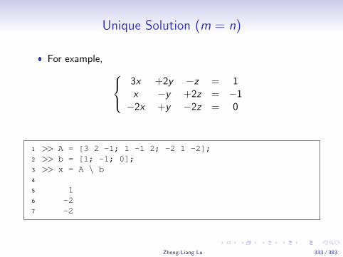
Unique Solution (m = n)
� For example, 3x +2y −z = 1x −y +2z = −1−2x +y −2z = 0
1 >> A = [3 2 -1; 1 -1 2; -2 1 -2];2 >> b = [1; -1; 0];3 >> x = A \ b4
5 16 -27 -2
Zheng-Liang Lu 333 / 383
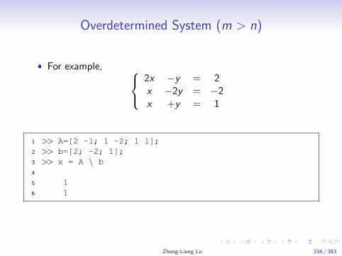
Overdetermined System (m > n)
� For example, 2x −y = 2x −2y = −2x +y = 1
1 >> A=[2 -1; 1 -2; 1 1];2 >> b=[2; -2; 1];3 >> x = A \ b4
5 16 1
Zheng-Liang Lu 334 / 383
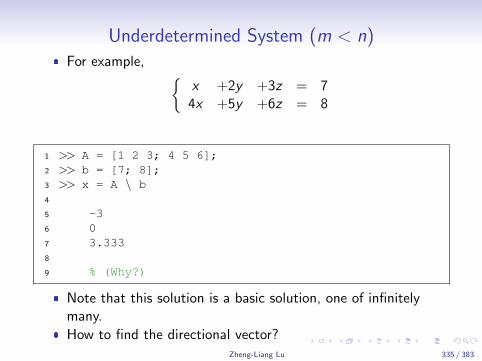
Underdetermined System (m < n)� For example, {
x +2y +3z = 74x +5y +6z = 8
1 >> A = [1 2 3; 4 5 6];2 >> b = [7; 8];3 >> x = A \ b4
5 -36 07 3.3338
9 % (Why?)
� Note that this solution is a basic solution, one of infinitelymany.
� How to find the directional vector?Zheng-Liang Lu 335 / 383
Gaussian Elimination
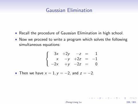
� Recall the procedure of Gaussian Elimination in high school.
� Now we proceed to write a program which solves the followingsimultaneous equations:
3x +2y −z = 1x −y +2z = −1
−2x +y −2z = 0
� Then we have x = 1, y = −2, and z = −2.
Zheng-Liang Lu 336 / 383
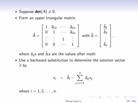
� Suppose det(A) 6= 0.
� Form an upper triangular matrix
A =
1 a12 · · · a1n0 1 · · · a2n...
... 1...
0 0 · · · 1
with b =
b1
b2...
bn
,where aijs and bi s are the values after math.
� Use a backward substitution to determine the solution vectorx by
xi = bi −n∑
j=i+1
aijxj ,
where i = 1, 2, · · · , n.
Zheng-Liang Lu 337 / 383
Solution
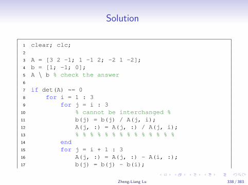
1 clear; clc;2
3 A = [3 2 -1; 1 -1 2; -2 1 -2];4 b = [1; -1; 0];5 A \ b % check the answer6
7 if det(A) ~= 08 for i = 1 : 39 for j = i : 3
10 % cannot be interchanged %11 b(j) = b(j) / A(j, i);12 A(j, :) = A(j, :) / A(j, i);13 % % % % % % % % % % % % % %14 end15 for j = i + 1 : 316 A(j, :) = A(j, :) - A(i, :);17 b(j) = b(j) - b(i);
Zheng-Liang Lu 338 / 383
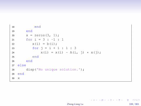
18 end19 end20 x = zeros(3, 1);21 for i = 3 : -1 : 122 x(i) = b(i);23 for j = i + 1 : 1 : 324 x(i) = x(i) - A(i, j) * x(j);25 end26 end27 else28 disp('No unique solution.');29 end30 x
Zheng-Liang Lu 339 / 383
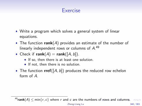
Exercise
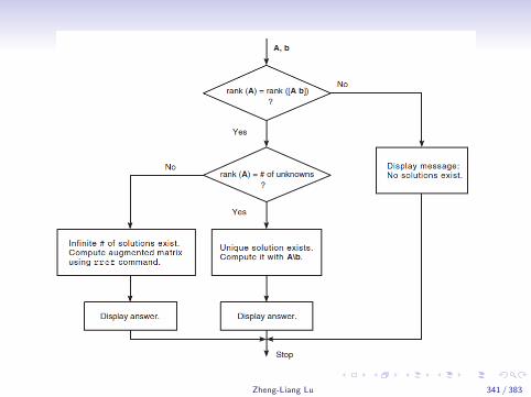
� Write a program which solves a general system of linearequations.
� The function rank(A) provides an estimate of the number oflinearly independent rows or columns of A.49
� Check if rank(A) = rank([A, b]).� If so, then there is at least one solution.� If not, then there is no solution.
� The function rref([A, b]) produces the reduced row echelonform of A.
49rank(A) ≤ min{r , c} where r and c are the numbers of rows and columns.Zheng-Liang Lu 340 / 383
Zheng-Liang Lu 341 / 383
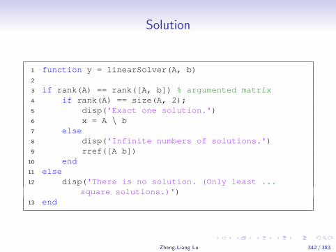
Solution
1 function y = linearSolver(A, b)2
3 if rank(A) == rank([A, b]) % argumented matrix4 if rank(A) == size(A, 2);5 disp('Exact one solution.')6 x = A \ b7 else8 disp('Infinite numbers of solutions.')9 rref([A b])
10 end11 else12 disp('There is no solution. (Only least ...
square solutions.)')13 end
Zheng-Liang Lu 342 / 383
Example: 2D Laplace’s Equation for Electrostatics
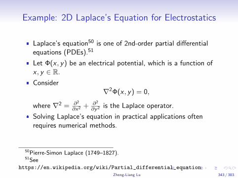
� Laplace’s equation50 is one of 2nd-order partial differentialequations (PDEs).51
� Let Φ(x , y) be an electrical potential, which is a function ofx , y ∈ R.
� Consider∇2Φ(x , y) = 0,
where ∇2 = ∂2
∂x2+ ∂2
∂y2 is the Laplace operator.
� Solving Laplace’s equation in practical applications oftenrequires numerical methods.
50Pierre-Simon Laplace (1749–1827).51See
https://en.wikipedia.org/wiki/Partial_differential_equation.Zheng-Liang Lu 343 / 383
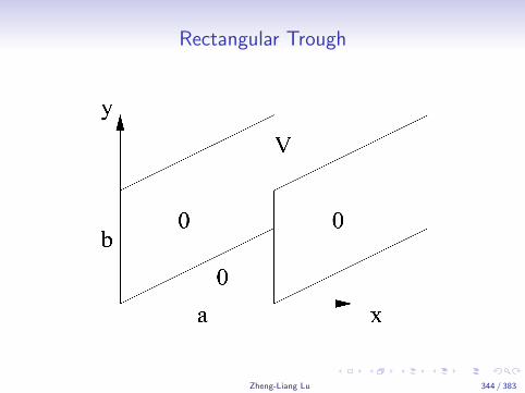
Rectangular Trough
Zheng-Liang Lu 344 / 383
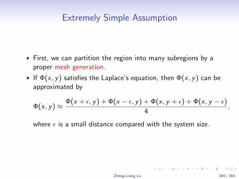
Extremely Simple Assumption
� First, we can partition the region into many subregions by aproper mesh generation.
� If Φ(x , y) satisfies the Laplace’s equation, then Φ(x , y) can beapproximated by
Φ(x , y) ≈ Φ(x + ε, y) + Φ(x − ε, y) + Φ(x , y + ε) + Φ(x , y − ε)4
,
where ε is a small distance compared with the system size.
Zheng-Liang Lu 345 / 383
0 0.1 0.2 0.3 0.4 0.5 0.6 0.7 0.8 0.9 10
0.1
0.2
0.3
0.4
0.5
0.6
0.7
0.8
0.9
1
V1
V2
V3
V4
V5
V6
V7
V8
V9
V10
V11
V12
V13
V14
V15
V16
V17
V18
V19
V20
V21
V22
V23
V24
V25
Zheng-Liang Lu 346 / 383
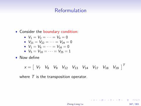
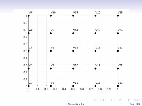
Reformulation
� Consider the boundary condition:� V1 = V2 = · · · = V4 = 0� V21 = V22 = · · · = V24 = 0� V1 = V6 = · · · = V16 = 0� V5 = V10 = · · · = V25 = 1
� Now define
x =[
V7 V8 V9 V12 V13 V14 V17 V18 V19
]Twhere T is the transposition operator.
Zheng-Liang Lu 347 / 383
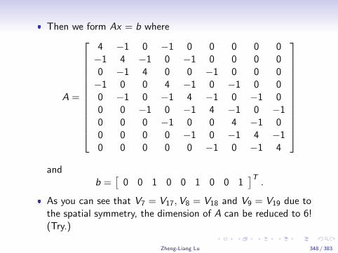
� Then we form Ax = b where
A =
4 −1 0 −1 0 0 0 0 0−1 4 −1 0 −1 0 0 0 00 −1 4 0 0 −1 0 0 0−1 0 0 4 −1 0 −1 0 00 −1 0 −1 4 −1 0 −1 00 0 −1 0 −1 4 −1 0 −10 0 0 −1 0 0 4 −1 00 0 0 0 −1 0 −1 4 −10 0 0 0 0 −1 0 −1 4
and
b =[
0 0 1 0 0 1 0 0 1]T.
� As you can see that V7 = V17,V8 = V18 and V9 = V19 due tothe spatial symmetry, the dimension of A can be reduced to 6!(Try.)
Zheng-Liang Lu 348 / 383
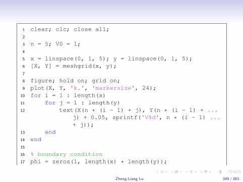
1 clear; clc; close all;2
3 n = 5; V0 = 1;4
5 x = linspace(0, 1, 5); y = linspace(0, 1, 5);6 [X, Y] = meshgrid(x, y);7
8 figure; hold on; grid on;9 plot(X, Y, 'k.', 'markersize', 24);
10 for i = 1 : length(x)11 for j = 1 : length(y)12 text(X(n * (i - 1) + j), Y(n * (i - 1) + ...
j) + 0.05, sprintf('V%d', n * (i - 1) ...+ j));
13 end14 end15
16 % boundary condition17 phi = zeros(1, length(x) * length(y));
Zheng-Liang Lu 349 / 383
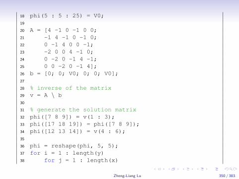
18 phi(5 : 5 : 25) = V0;19
20 A = [4 -1 0 -1 0 0;21 -1 4 -1 0 -1 0;22 0 -1 4 0 0 -1;23 -2 0 0 4 -1 0;24 0 -2 0 -1 4 -1;25 0 0 -2 0 -1 4];26 b = [0; 0; V0; 0; 0; V0];27
28 % inverse of the matrix29 v = A \ b30
31 % generate the solution matrix32 phi([7 8 9]) = v(1 : 3);33 phi([17 18 19]) = phi([7 8 9]);34 phi([12 13 14]) = v(4 : 6);35
36 phi = reshape(phi, 5, 5);37 for i = 1 : length(y)38 for j = 1 : length(x)
Zheng-Liang Lu 350 / 383
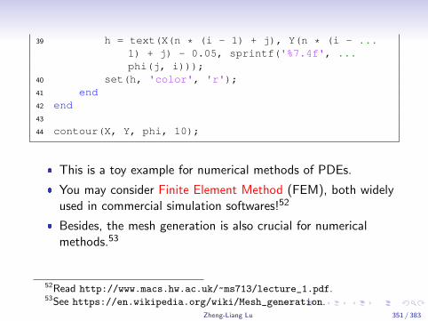
39 h = text(X(n * (i - 1) + j), Y(n * (i - ...1) + j) - 0.05, sprintf('%7.4f', ...phi(j, i)));
40 set(h, 'color', 'r');41 end42 end43
44 contour(X, Y, phi, 10);
� This is a toy example for numerical methods of PDEs.
� You may consider Finite Element Method (FEM), both widelyused in commercial simulation softwares!52
� Besides, the mesh generation is also crucial for numericalmethods.53
52Read http://www.macs.hw.ac.uk/~ms713/lecture_1.pdf.53See https://en.wikipedia.org/wiki/Mesh_generation.
Zheng-Liang Lu 351 / 383

0 0.1 0.2 0.3 0.4 0.5 0.6 0.7 0.8 0.9 10
0.1
0.2
0.3
0.4
0.5
0.6
0.7
0.8
0.9
1
V1
V2
V3
V4
V5
V6
V7
V8
V9
V10
V11
V12
V13
V14
V15
V16
V17
V18
V19
V20
V21
V22
V23
V24
V25
0.0000
0.0000
0.0000
0.0000
1.0000
0.0000
0.0714
0.1875
0.4286
1.0000
0.0000
0.0982
0.2500
0.5268
1.0000
0.0000
0.0714
0.1875
0.4286
1.0000
0.0000
0.0000
0.0000
0.0000
1.0000
Zheng-Liang Lu 352 / 383
Method of Least Squares
� The first clear and concise exposition of the method of leastsquares was published by Legendre in 1805.
� In 1809, Gauss published his method of calculating the orbitsof celestial bodies.
� The method of least squares is a standard approach to theapproximate solution of overdetermined systems, that is, setsof equations in which there are more equations thanunknowns.54
� To obtain the coefficient estimates, the least-squares methodminimizes the summed square of residuals.
54Aka degrees of freedom.Zheng-Liang Lu 353 / 383
� Let {yi}ni=1 be the observed response values and {yi}ni=1 bethe fitted response values.
� Let εi = yi − yi be the residual for i = 1, . . . , n.
� Then the sum of square error estimates associated with thedata is given by
S =n∑
i=1
ε2i .
Zheng-Liang Lu 354 / 383
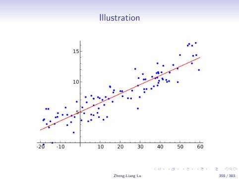
Illustration
Zheng-Liang Lu 355 / 383
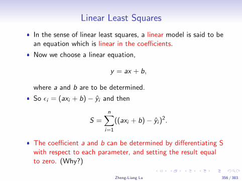
Linear Least Squares
� In the sense of linear least squares, a linear model is said to bean equation which is linear in the coefficients.
� Now we choose a linear equation,
y = ax + b,
where a and b are to be determined.
� So εi = (axi + b)− yi and then
S =n∑
i=1
((axi + b)− yi )2.
� The coefficient a and b can be determined by differentiating Swith respect to each parameter, and setting the result equalto zero. (Why?)
Zheng-Liang Lu 356 / 383
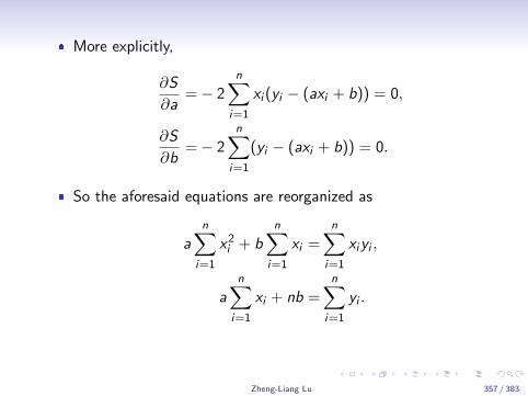
� More explicitly,
∂S
∂a=− 2
n∑i=1
xi (yi − (axi + b)) = 0,
∂S
∂b=− 2
n∑i=1
(yi − (axi + b)) = 0.
� So the aforesaid equations are reorganized as
an∑
i=1
x2i + b
n∑i=1
xi =n∑
i=1
xiyi ,
an∑
i=1
xi + nb =n∑
i=1
yi .
Zheng-Liang Lu 357 / 383
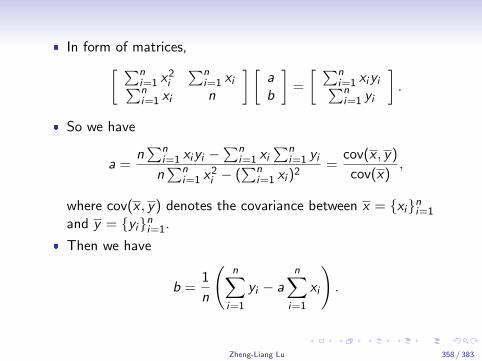
� In form of matrices,[ ∑ni=1 x2
i
∑ni=1 xi∑n
i=1 xi n
] [ab
]=
[ ∑ni=1 xiyi∑ni=1 yi
].
� So we have
a =n∑n
i=1 xiyi −∑n
i=1 xi∑n
i=1 yin∑n
i=1 x2i − (
∑ni=1 xi )2
=cov(x , y)
cov(x),
where cov(x , y) denotes the covariance between x = {xi}ni=1
and y = {yi}ni=1.
� Then we have
b =1
n
(n∑
i=1
yi − an∑
i=1
xi
).
Zheng-Liang Lu 358 / 383

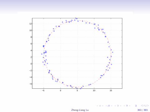
Example: Circle Fitting
� Consider a set of data points surrounding some center.
� Now the coordinates of the circle center and also the radiusare desired.
� This needs to estimate 3 unknowns: (xc , yc) and r > 0.
� Recall that a circle equation is (x − xc)2 + (y − yc)2 = r2.
� The above equation can be equivalent to
2xxc + 2yyc + z = x2 + y2,
wherez = r2 − x2
c + y2c .
Zheng-Liang Lu 359 / 383

� For a set of data points (xi , yi ), i = 1, 2, 3, . . . ,N, thisrearranged equation can be written in matrix form
Aw = b,
where
A =
2x1 2y1 1...
. . ....
2xN 2yN 1
,w =
xcycz
, b =
x21 + y2
1...
x2N + y2
N
.
Zheng-Liang Lu 360 / 383
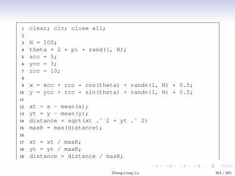
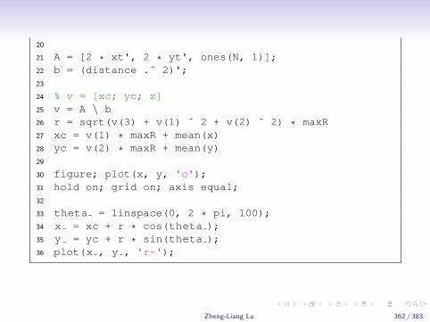
1 clear; clc; close all;2
3 N = 100;4 theta = 2 * pi * rand(1, N);5 xcc = 5;6 ycc = 3;7 rcc = 10;8
9 x = xcc + rcc * cos(theta) + randn(1, N) * 0.5;10 y = ycc + rcc * sin(theta) + randn(1, N) * 0.5;11
12 xt = x - mean(x);13 yt = y - mean(y);14 distance = sqrt(xt .ˆ 2 + yt .ˆ 2)15 maxR = max(distance);16
17 xt = xt / maxR;18 yt = yt / maxR;19 distance = distance / maxR;
Zheng-Liang Lu 361 / 383
20
21 A = [2 * xt', 2 * yt', ones(N, 1)];22 b = (distance .ˆ 2)';23
24 % v = [xc; yc; z]25 v = A \ b26 r = sqrt(v(3) + v(1) ˆ 2 + v(2) ˆ 2) * maxR27 xc = v(1) * maxR + mean(x)28 yc = v(2) * maxR + mean(y)29
30 figure; plot(x, y, 'o');31 hold on; grid on; axis equal;32
33 theta = linspace(0, 2 * pi, 100);34 x = xc + r * cos(theta );35 y = yc + r * sin(theta );36 plot(x , y , 'r-');
Zheng-Liang Lu 362 / 383
−5 0 5 10 15
−6
−4
−2
0
2
4
6
8
10
12
Zheng-Liang Lu 363 / 383
Polynomials55
� In fact, all polynomials of n-th order with addition andmultiplication to scalars form a vector space, denoted by Pn.
� In general, f (x) is said to be a polynomial of n-order providedthat
f (x) = anxn + an−1xn−1 + · · ·+ a0,
where an 6= 0.
� It is convenient to express a polynomial by a coefficient vector(an, an−1, . . . , a0), where the elements are the coefficients ofthe polynomial in descending order.
55Weierstrass approximation theorem states that every continuous functiondefined on a closed interval [a, b] can be uniformly approximated as closely asdesired by a polynomial function. Seehttps://en.wikipedia.org/wiki/Stone_Weierstrass_theorem.
Zheng-Liang Lu 364 / 383
Arithmetic Operations
� P1 + P2 returns the addition of two polynomials.
� P1 − P2 returns the subtraction of two polynomials.
� The function conv(P1,P2) returns the resulting coefficientvector for multiplication of the two polynomials P1 and P2.56
� The function [Q,R] = deconv(B,A) deconvolves vector Aout of vector B.
� Equivalently, B = conv(A,Q) + R.� This is so-called “Euclidean division algorithm.”
� The function polyval(P,X ) returns the values of a polynomialP evaluated at x ∈ X .
56See Convolution.Zheng-Liang Lu 365 / 383
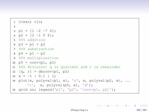
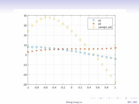
1 clear; clc;2
3 p1 = [1 -2 -7 4];4 p2 = [2 -1 0 6];5 %%% addition6 p3 = p1 + p27 %%% substraction8 p4 = p1 - p29 %%% multiplcaition
10 p5 = conv(p1, p2)11 %%% division: q is quotient and r is remainder12 [q, r] = deconv(p1, p2)13 x = -1 : 0.1 : 1;14 plot(x, polyval(p1, x), 'o', x, polyval(p2, x), ...
'*', x, polyval(p5, x), 'd');15 grid on; legend('p1', 'p2', 'conv(p1, p2)');
Zheng-Liang Lu 366 / 383
-1 -0.8 -0.6 -0.4 -0.2 0 0.2 0.4 0.6 0.8 1-30
-20
-10
0
10
20
30
40
p1p2conv(p1, p2)
Zheng-Liang Lu 367 / 383
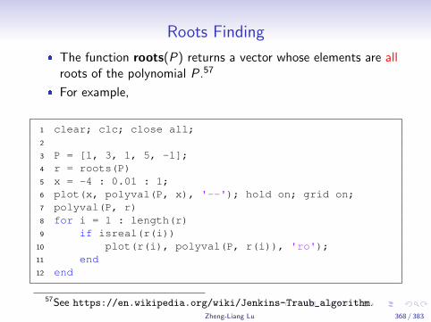
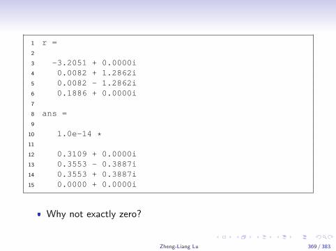
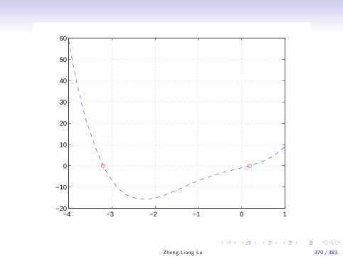
Roots Finding
� The function roots(P) returns a vector whose elements are allroots of the polynomial P.57
� For example,
1 clear; clc; close all;2
3 P = [1, 3, 1, 5, -1];4 r = roots(P)5 x = -4 : 0.01 : 1;6 plot(x, polyval(P, x), '--'); hold on; grid on;7 polyval(P, r)8 for i = 1 : length(r)9 if isreal(r(i))
10 plot(r(i), polyval(P, r(i)), 'ro');11 end12 end
57See https://en.wikipedia.org/wiki/Jenkins-Traub_algorithm.Zheng-Liang Lu 368 / 383
1 r =2
3 -3.2051 + 0.0000i4 0.0082 + 1.2862i5 0.0082 - 1.2862i6 0.1886 + 0.0000i7
8 ans =9
10 1.0e-14 *11
12 0.3109 + 0.0000i13 0.3553 - 0.3887i14 0.3553 + 0.3887i15 0.0000 + 0.0000i
� Why not exactly zero?
Zheng-Liang Lu 369 / 383
−4 −3 −2 −1 0 1−20
−10
0
10
20
30
40
50
60
Zheng-Liang Lu 370 / 383
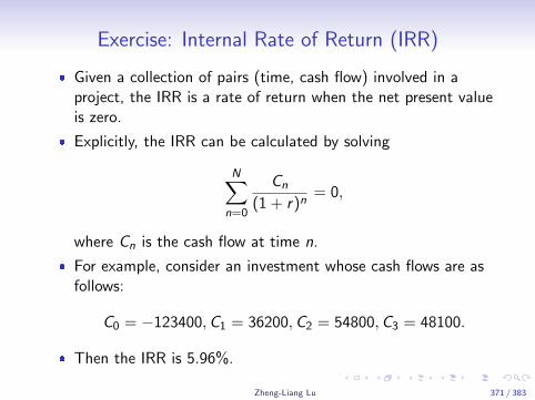
Exercise: Internal Rate of Return (IRR)
� Given a collection of pairs (time, cash flow) involved in aproject, the IRR is a rate of return when the net present valueis zero.
� Explicitly, the IRR can be calculated by solving
N∑n=0
Cn
(1 + r)n= 0,
where Cn is the cash flow at time n.
� For example, consider an investment whose cash flows are asfollows:
C0 = −123400,C1 = 36200,C2 = 54800,C3 = 48100.
� Then the IRR is 5.96%.
Zheng-Liang Lu 371 / 383
Forming Polynomials
� The function poly(V ), where V is a vector, returns a vectorwhose elements are the coefficients of the polynomial whoseroots are the elements of V .
� Simply put, the function roots and poly are inverse functionsof each other.
Zheng-Liang Lu 372 / 383

Example
1 clear; clc;2
3 v = [0.5 sqrt(2) 3];4 y = 1;5 for i = 1 : 36 y = conv(y, [1 -v(i)]);7 end8 y9
10 poly(v)
Zheng-Liang Lu 373 / 383
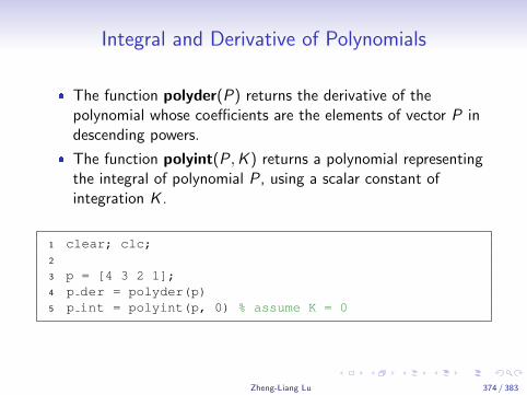
Integral and Derivative of Polynomials
� The function polyder(P) returns the derivative of thepolynomial whose coefficients are the elements of vector P indescending powers.
� The function polyint(P,K ) returns a polynomial representingthe integral of polynomial P, using a scalar constant ofintegration K .
1 clear; clc;2
3 p = [4 3 2 1];4 p der = polyder(p)5 p int = polyint(p, 0) % assume K = 0
Zheng-Liang Lu 374 / 383
Exercise
� Consider f (x) = 4x3 + 3x2 + 2x + 1 for x ∈ R.
� Determine the coefficients of its derivative f ′ and integrationF (x) =
∫ x0 f (t)dt.
� Do not use the built-in functions.
Zheng-Liang Lu 375 / 383

1 clear; clc;2
3 p = randi(100, 1, 4)4 q1 = [0, p(1 : end - 1) .* [length(p) - 1 : -1 : 1]]5 q2 = [p ./ [length(p) : -1 : 1], 0]6
7 T1 = [0 0 0 0;8 3 0 0 0;9 0 2 0 0;
10 0 0 1 0];11 T1 * p'12 T2 = [0 1/4 0 0 0;13 0 0 1/3 0 0;14 0 0 0 1/2 0;15 0 0 0 0 1;16 0 0 0 0 0];17 T2 * [0 p]'
Zheng-Liang Lu 376 / 383
Curve Fitting by Polynomials
� The function polyfit(x , y , n) returns the coefficients for apolynomial p(x) of degree n that is a best fit (in aleast-squares sense) for the data in y .
Zheng-Liang Lu 377 / 383
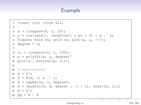
Example
1 clear; clc; close all;2
3 x = linspace(0, 1, 10);4 y = cos(rand(1, length(x)) * pi / 2) + x .ˆ 2;5 figure; hold on; grid on; plot(x, y, 'o');6 degree = 5;7
8 x = linspace(0, 1, 100);9 p = polyfit(x, y, degree)'
10 plot(x , polyval(p, x ));11
12 % equivalence13 x = x';14 f = @(x, i) x .ˆ i;15 A = repmat(x, 1, degree);16 A = [bsxfun(f, A, degree : -1 : 1), ones(10, 1)];17 b = y';18 pp = A \ b
Zheng-Liang Lu 378 / 383
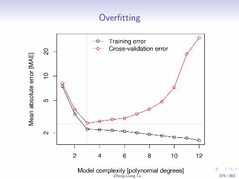
Overfitting
Zheng-Liang Lu 379 / 383
Occam’s Razor
“Entities must not be multiplied beyond necessity.”– Duns Scotus
� In science, Occam’s razor is used as a heuristic to guidescientists in developing theoretical models rather than as anarbiter between published models.
� Among competing hypotheses, the one with the fewestassumptions should be selected.
� For example, Runge’s phenomenon is a problem of oscillationat the edges of an interval that occurs when using polynomialinterpolation with polynomials of high degree over a set ofequispaced interpolation points.58
58See https://en.wikipedia.org/wiki/Runge’s_phenomenon.Zheng-Liang Lu 380 / 383
Eigenvalues and Eigenvectors59
� Let A be a square matrix.
� Then v is an eigenvector associated with the eigenvalue λ if
Av = λv .
� Equivalently,(A− λI )v = 0.
� For nontrivial vectors v , det(A− λI ) = 0.
� The above equation is the so-called characteristic polynomial,whose roots are actually eigenvalues!
� Use eig(A) to derive the eigenvalues associated witheigenvectors for the matrix A.
59See https:
//en.wikipedia.org/wiki/Eigenvalues_and_eigenvectors#Applications
and https://en.wikipedia.org/wiki/Eigenvalue_algorithm.Zheng-Liang Lu 381 / 383
Singular Value Decomposition (SVD)60
� Let Am×n be a matrix.
� Then σ is called one singular value associated with thesingular vectors u ∈ Rm×1 and v ∈ Rn×1 for A provided that{
Av = σu,ATu = σv .
� We further have {AV = UΣ,
ATU = V Σ,
where U and V are both unitary, and the diagonal terms in Σare σ’s, 0’s in off-diagonal terms.
� You may use the built-in function svd.
60Seehttps://www.mathworks.com/help/matlab/math/singular-values.html.
Zheng-Liang Lu 382 / 383
Example: Low-rank Approximation for Image Compression
� This idea originates from Principal Component Analysis(PCA).61
� Use svd to calculate the principal components of the inputimage.
� Then we can have an image extremely similar to the originone, but with a smaller image size by keeping the vectorsassociated with a few first largest of principal components.
61See https://www.cs.princeton.edu/picasso/mats/
PCA-Tutorial-Intuition_jp.pdf andhttp://setosa.io/ev/principal-component-analysis/.
Zheng-Liang Lu 383 / 383