Embed Size (px)
Citation preview

Clemson UniversityTigerPrints
All Theses Theses
8-2014
Fatigue-Induced Failure in Horizontal-Axis Wind-Turbine (HAWT) Blades and HAWT DrivetrainGearsVarun ChennaClemson University, [email protected]
Follow this and additional works at: https://tigerprints.clemson.edu/all_theses
Part of the Mechanical Engineering Commons
This Thesis is brought to you for free and open access by the Theses at TigerPrints. It has been accepted for inclusion in All Theses by an authorizedadministrator of TigerPrints. For more information, please contact [email protected].
Recommended CitationChenna, Varun, "Fatigue-Induced Failure in Horizontal-Axis Wind-Turbine (HAWT) Blades and HAWT Drivetrain Gears" (2014).All Theses. 1863.https://tigerprints.clemson.edu/all_theses/1863

TITLE PAGE
FATIGUE–INDUCED FAILURE IN
HORIZONTAL–AXIS WIND–TURBINE (HAWT)
BLADES AND HAWT DRIVETRAIN GEARS
A Thesis
Presented to
the Graduate School of
Clemson University
In Partial Fulfillment
of the Requirements for the Degree
Master of Science
Mechanical Engineering
by
Varun Chenna
August 2014
Accepted by:
Dr. Mica Grujicic, Committee Chair
Dr. Chenning Tong
Dr. Jay Ochterbeck

II
ABSTRACT
Wind energy is one of the most promising and the fastest growing installed alternative-
energy production technologies. In fact, it is anticipated that by 2030, at least 20% of the U.S.
energy needs will be met by various onshore and offshore wind-farms [a collection of wind-
turbines (converters of wind energy into electrical energy) at the same location]. A majority of
wind turbines nowadays fall into the class of the so-called Horizontal Axis Wind Turbines
(HAWTs).
Turbine blades and the gearbox are perhaps the most critical components/subsystems in
the present designs of HAWTs. The combination of high failure rates (particularly those
associated with turbine-blades and gear-boxes), long downtimes and the high cost of repair
remains one of the major problems to the wind-energy industry today.
In the case of HAWT blades, one is typically concerned about the following two quasi-
static structural-performance requirements: (a) sufficient “flap-wise” bending strength to
withstand highly-rare extreme static-loading conditions (e.g., 50-year return-period gust, a short
strong blast of wind); and (b) sufficient turbine blade “flap-wise” bending stiffness in order to
ensure that a minimal clearance is maintained between blade tip and the turbine tower at all times
during wind turbine operation. If these two structural requirements are not met, HAWT blades
typically fail prematurely. In addition to the aforementioned quasi-static structural-performance
requirements, one is also concerned about the premature-failure caused by inadequate fatigue-
based durability of the HAWT blades. The durability requirement for the turbine blades is
typically defined as a minimum of 20-year fatigue life (which corresponds roughly to ca. 108
cycles) when subjected to stochastic wind-loading conditions and cyclic gravity-induced edge-
wise bending loads in the presence of thermally-fluctuating and environmentally challenging

III
conditions. In the present work, a computational framework has been developed to address: (a)
structural response of HAWT blades subjected to extreme loading conditions; (b) high-cycle-
fatigue-controlled durability of the HAWT blades; and (c) methodology for HAWT-blade
material selection. To validate the computational approach used, key results are compared with
their experimental counterparts available in the public-domain literature.
As far as the HAWT gear-boxes are concerned, while they are designed for the entire life
(ca. 20 years) of the HAWT, in practice, most gear-boxes have to be repaired or even overhauled
considerably earlier (3–5 years). Typically, a HAWT gear-box fails either due to the bending-
fatigue-induced failure of its gears, or by tribo-chemical degradation and failure of its bearings. In
the present work, a computational framework has been developed to predict HAWT service-life
under extreme loading and unfavorable kinematic conditions, for the case when the gear-box
service-life is controlled by gear-tooth bending-fatigue failure. In addition, a preliminary
investigation of gear-box bearing kinematics, which can result in undesirable rolling-element
skidding conditions, is conducted.
Keywords: Horizontal Axis Wind Turbine, Composite Material Selection, Fatigue Life
Assessment, Gearbox Reliability

IV
DEDICATION
This thesis would have been impossible without the unwavering love and support from
my father, Mr. Keshava Chand Chenna, my mother, Mrs. Uma Rani Chenna, and my sister
Yeshashwini Chenna to whom this thesis is dedicated.

V
ACKNOWLEDGEMENTS
I wish to express my sincere gratitude to my advisor, Professor Mica Grujicic, for his
continuous encouragement, supervision, useful suggestions, and support throughout this research
endeavor. His extensive knowledge and timely suggestions have been helpful in providing
elegant solutions to the problems encountered throughout this research project.
My sincere thanks is also due to my advisory committee members Professor Chenning
Tong, and Professor Jay Ochterbeck for their valuable suggestions during the course of this
research project. Other faculty members of the department of Mechanical Engineering at
Clemson University and the administrative staff are also greatly acknowledged for their support.
This acknowledgement will not be complete without the mention of my friends and
colleagues at Clemson University whose valuable support and insightful discussions have helped
mold this research into its existing form. Finally, I would like to thank my family and friends for
their continuous support and encouragement during the whole tenure of my research.

VI
TABLE OF CONTENTS
Page
TITLE PAGE ................................................................................................................................... I
ABSTRACT .................................................................................................................................... II
DEDICATION .............................................................................................................................. IV
ACKNOWLEDGEMENTS ............................................................................................................ V
LIST OF TABLES .......................................................................................................................... X
LIST OF FIGURES ....................................................................................................................... XI
CHAPTER
CHAPTER 1: INTRODUCTION AND BACKGROUND, AND THESIS OUTLINE ............ 1
1.1. Introduction and Background ................................................................................ 1
1.2 Thesis Outline ......................................................................................................... 6
1.3 References ............................................................................................................... 7
CHAPTER 2: HORIZONTAL–AXIS WIND–TURBINE BLADES: STRUCTURAL–
RESPONSE ANALYSIS, FATIGUE–LIFE PREDICTION, AND MATERIAL
SELECTION ....................................................................................................................... 8
2.1. Abstract .................................................................................................................. 8
2.2. Introduction ............................................................................................................ 9
2.2.1 Wind Energy ...................................................................................................... 10
2.2.2 Structural/Dynamics Requirements for HAWTs and HAWT Blades ................ 12
2.2.3 Typical Construction of HAWTs and HAWT Blades ....................................... 14

VII
Table of Contents (Continued)
Page
2.2.4 Main Objectives ................................................................................................. 18
2.2.5 Chapter Organization ......................................................................................... 19
2.3. Computational Methods and Tools ...................................................................... 20
2.3.1 Geometrical and Meshed Models ...................................................................... 20
2.3.2 Wind-Turbine Blade Structural Analysis ........................................................... 24
2.3.3 Wind-Turbine Blade Fatigue-Life Prediction .................................................... 29
2.3.4 Wind-Turbine Blade Material Selection ............................................................ 37
2.4. Results and Discussion ........................................................................................ 40
2.4.1 The Baseline Case .............................................................................................. 42
2.4.2 HAWT-Blade Design Modifications ................................................................. 57
2.4.3 HAWT-Blade Material Selection ...................................................................... 59
2.5. Summary and Conclusions .................................................................................. 65
2.6. References ............................................................................................................ 66
CHAPTER 3: HORIZONTAL–AXIS WIND–TURBINE: GEAR–BOX FAILURE VIA
TOOTH–BENDING FATIGUE ....................................................................................... 67
3.1. Abstract ................................................................................................................ 67
3.2. Introduction .......................................................................................................... 68
3.2.1 Wind Energy Harvesting.................................................................................... 69
3.2.2 Wind Turbine Gearbox Reliability .................................................................... 71
3.2.3 Main Modes of Gear Damage and Failure ......................................................... 74
3.2.4 Main Objectives ................................................................................................. 76

VIII
Table of Contents (Continued)
Page
3.2.5 Chapter Organization ......................................................................................... 78
3.3. Finite-Element Stress Analysis ............................................................................ 79
3.3.1 Problem Formulation ......................................................................................... 80
3.3.2 Computational Analysis ..................................................................................... 81
3.4. Fatigue Strength and Life-Cycle Prediction......................................................... 86
3.4.1 Fatigue-Crack Initiation ..................................................................................... 87
3.4.2 Fatigue-Crack Growth ....................................................................................... 89
3.5. Results and Discussion ........................................................................................ 91
3.5.1 Temporal Evolution/Spatial Distribution of Gear-Tooth Stresses ..................... 92
3.5.2 Fatigue-Life Prediction .................................................................................... 102
3.6. Summary and Conclusions ................................................................................ 106
3.7. References .......................................................................................................... 107
CHAPTER 4: HORIZONTAL–AXIS WIND–TURBINE: PRELIMINARY BEARING
KINEMATICS AND KINETICS ................................................................................... 109
4.1. Abstract .............................................................................................................. 109
4.2. Introduction ........................................................................................................ 110
4.2.1 Wind Energy Harvesting.................................................................................. 111
4.2.2 Wind Turbine Gear-box Reliability ................................................................. 113
4.2.3 Premature Failure of Wind-Turbine Gear-box Roller-Bearings ...................... 116
4.2.4 Main Objectives ............................................................................................... 119
4.3. Multibody Dynamics of a Gearbox Roller Bearing ........................................... 120

IX
Table of Contents (Continued)
Page
4.3.1 Problem Description ........................................................................................ 120
4.3.2 SIMPACK Computer Program ........................................................................ 122
4.3.3 Roller-Bearing MBD Model ............................................................................ 123
4.3.4 Construction of the User-defined Force Element ............................................ 139
4.3.5 Kinematics-based Derivation of the Zero-Slip Roller Angular Velocity ......... 140
4.4. Results and Discussion ...................................................................................... 142
4.5. Summary and Conclusions ................................................................................ 147
4.6. References .......................................................................................................... 148
CHAPTER 5: CONCLUSIONS AND SUGGESTIONS FOR FUTURE WORK ................ 149
5.1. Conclusions ........................................................................................................ 149
5.2. Suggestions for Future Work ............................................................................. 151
APPENDIX A: User-defined Force Element – uforce20 source code................................... 152

X
LIST OF TABLES
Table Page
Table 2-1 HAWT-Blade Composite-laminate Lay-up Sequence ............................................... 45
Table 2-2 Summary of the HAWT-Blade Material Properties ................................................... 46
Table 4-1 Specifications of multi-body model of cylindrical roller bearing ............................. 126
Table 4-2 Types of joints used in the MBS model .................................................................... 127
Table 4-3 Relationship between the dimensionless contact parameters [11] ............................ 130

XI
LIST OF FIGURES
Figure Page
Figure 1-1 A photograph of a typical off-shore wind farm, with the major wind turbine
sub-systems identified [8] ................................................................................................ 2
Figure 2-1 Variation of the horizontal-axis wind turbine power output and rotor
diameter with the year of deployment. ........................................................................... 11
Figure 2-2 Typical off-shore wind farm. The major wind turbine sub-systems are
identified [16]. ................................................................................................................ 15
Figure 2-3 Typical turbine-blade cross-sectional area in the case of: (a) the one-piece
construction; and (b) the two-piece construction. .......................................................... 17
Figure 2-4 Typical: (a) geometrical and (b) meshed models of a single wind-turbine
blade analyzed in the present work. ............................................................................... 22
Figure 2-5 An example of the results pertaining to the 2-dimensional distribution of the
coefficient of pressure and the streamlines in the region surrounding the airfoil
for the case of a 100 angle of attack (the angle between the wind direction and
the airfoil chord. ............................................................................................................. 26
Figure 2-6 (a) Application of the rainflow cycle-counting algorithm to a simple load
signal after the peak/valley reconstruction. Please see text for explanation; and
(b) the resulting three dimensional histogram showing the number of cycles /
half-cycles in each mean stress/strain – stress/strain amplitude bin. ............................. 31

XII
List of Figures (Continued)
Figure Page
Figure 2-7 An example of the Goodman diagram showing constant fatigue-life data
(dashed lines) and constant R-ratio data (the solid lines emanating from the
origin). ............................................................................................................................ 33
Figure 2-8 An example of the three-dimensional histogram showing the effect of
stress/strain amplitude and the stress/strain mean-value of the material fatigue
life. ................................................................................................................................. 35
Figure 2-9 Baseline case of the HAWT blade analyzed in the present work: (a) the
airfoil cross section; and (b) the planform. .................................................................... 43
Figure 2-10 Displacement magnitude distribution over the HAWT blade outer skin
caused by a 70m/s gust: (a) the baseline case; and (b) a modified-design case. ............ 48
Figure 2-11 Variation of the gust-induced HAWT-blade thickness for the blade designs
analyzed in the present work. ......................................................................................... 50
Figure 2-12 Von Mises equivalent stress distribution over the HAWT interior structural
members (spar-cap and shear-webs) caused by a 70m/s gust: (a) the baseline
case; and (b) a modified-design case. ............................................................................ 52
Figure 2-13 Variation of the gust-induced HAWT-blade twist angle for the blade
designs analyzed in the present work. ............................................................................ 54
Figure 2-14 Material property charts used in the HAWT-blade material selection
process. Please see text for details. ................................................................................ 62

XIII
List of Figures (Continued)
Figure Page
Figure 3-1 Schematic of a prototypical wind-turbine gearbox. The major components
and sub-systems are identified. ...................................................................................... 73
Figure 3-2 (a) Geometrical model; and (b) Close-up of the meshed model consisting of
two helical gears and two shafts, used in the present work............................................ 82
Figure 3-3 Typical temporal evolution and spatial distribution of the maximum
principal stress over the surface of a tooth of the driven gear (for the case of
perfectly aligned shafts). ................................................................................................ 93
Figure 3-4 The effect of the torque transferred by the gear-pair analyzed on the largest
value of the maximum principal stress in the subject gear-tooth). ................................. 96
Figure 3-5 The effect of shaft misalignment (as quantified by the corresponding
misalignment angle, ), at a constant level of the transferred-torque, on the
spatial distribution and the magnitude of the gear-tooth maximum principal
stress, at the instant when the subject gear-tooth experiences the largest value
of the maximum principal stress: (a) = 0°; (b) = 1°; (c) = 2°; and (d) =
3°. ................................................................................................................................... 98
Figure 3-6 The effect of the gear-misalignment angle, at a constant level of the
transferred-torque, on the largest values of the maximum principal stress. ................. 101
Figure 3-7 The effect of the transferred-torque on the total service-life of the driven
helical gear, for the case of perfectly aligned gears. .................................................... 104

XIV
List of Figures (Continued)
Figure Page
Figure 3-8 The effect of the misalignment angle on the total fatigue-controlled service-
life of the driven helical gear, under a constant transferred-torque condition. ............ 105
Figure 4-1 Schematic of a prototypical wind-turbine gear-box. The major components
and sub-systems are identified. Failure typically occurs within the (planet,
intermediate-speed shaft and high-speed shaft) roller-bearings. .................................. 115
Figure 4-2 A labeled CAD model of the roller bearing MBD model analyzed. ....................... 125
Figure 4-3 The effect of rolling-element/race slip velocity on the coefficient of friction
under elastohydrodynamic conditions [10]. ................................................................. 132
Figure 4-4 A schematic of the single-roller/inner-race contact pair used to explain the
way the contact-interaction torque is calculated within uforce20 and returned to
SIMPACK. ................................................................................................................... 136
Figure 4-5 The effect of the inner-race rotational speed and the outer-race rotational
speed on the no-slip revolving velocity of the rollers in the case of the roller-
bearing being analyzed: (a) an analytical kinematics-based solution; and (b) the
numerical uforce20/SIMPACK based solution. ........................................................... 143
Figure 4-6 The effect of the inner-race rotational speed and the outer-race rotational
speed on the no-slip angular (rotational) velocity of the rollers in the case of
the roller-bearing being analyzed: (a) an analytical kinematics-based solution;
and (b) the numerical uforce20/SIMPACK based solution. ........................................ 144

XV
List of Figures (Continued)
Figure Page
Figure 4-7 The effect of (constant) inner-race rotational velocity, for the case of the
initially stationary rolling elements and always stationary outer race, at the
interfaces between the rolling elements and: (a) the inner race; (b) the outer
race. .............................................................................................................................. 146

1
CHAPTER 1: INTRODUCTION AND BACKGROUND, AND THESIS OUTLINE
1.1. Introduction and Background
Wind energy is one of the most promising and the fastest growing installed alternative-
energy production technologies. In fact, it is anticipated that by 2030, at least 20% of the U.S.
energy needs will be met by various onshore and offshore wind-farms [a collection of wind-
turbines (converters of wind energy into electrical energy) at the same location] [1]. A majority of
wind turbines nowadays fall into the class of the so-called Horizontal Axis Wind Turbines
(HAWTs). Typically, a HAWT consists of the following key functional components/assemblies:
(a) rotor – consisting of three (for increased structural stability and aerodynamic efficiency)
aerodynamically-shaped blades; (b) drive-train – consisting of an input/low-speed shaft, a gear-
box and output/high-speed shaft; (c) electrical generator – the rotor of which is attached to the
high-speed shaft; (d) nacelle – the housing of the drive-train and electrical generator; (e) bedplate
– to which the drive-train, electrical generator and nacelle are mounted; and (f) tower – a tall,
slender structure on the top of which the bedplate is mounted. A photograph of an offshore wind
turbine is provided in Figure 1-1. All major components of the turbine are labeled for
identification.

2
Figure 1-1 A photograph of a typical off-shore wind farm, with the major wind turbine sub-systems
identified [8]
Rotor
Hub
Nacelle
Tower
3
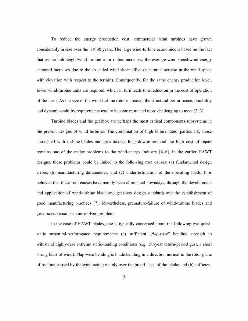
To reduce the energy production cost, commercial wind turbines have grown
considerably in size over the last 30 years. The large wind-turbine economics is based on the fact
that as the hub-height/wind-turbine rotor radius increases, the average wind-speed/wind-energy
captured increases due to the so called wind shear effect (a natural increase in the wind speed
with elevation with respect to the terrain). Consequently, for the same energy production level,
fewer wind-turbine units are required, which in turn leads to a reduction in the cost of operation
of the farm. As the size of the wind-turbine rotor increases, the structural performance, durability
and dynamic-stability requirements tend to become more and more challenging to meet [2, 3].
Turbine blades and the gearbox are perhaps the most critical components/subsystems in
the present designs of wind turbines. The combination of high failure rates (particularly those
associated with turbine-blades and gear-boxes), long downtimes and the high cost of repair
remains one of the major problems to the wind-energy industry [4–6]. In the earlier HAWT
designs, these problems could be linked to the following root causes: (a) fundamental design
errors; (b) manufacturing deficiencies; and (c) under-estimation of the operating loads. It is
believed that these root causes have mainly been eliminated nowadays, through the development
and application of wind-turbine blade and gear-box design standards and the establishment of
good manufacturing practices [7]. Nevertheless, premature-failure of wind-turbine blades and
gear-boxes remains an unresolved problem.
In the case of HAWT blades, one is typically concerned about the following two quasi-
static structural-performance requirements: (a) sufficient “flap-wise” bending strength to
withstand highly-rare extreme static-loading conditions (e.g., 50-year return-period gust, a short
strong blast of wind). Flap-wise bending is blade bending in a direction normal to the rotor plane
of rotation caused by the wind acting mainly over the broad faces of the blade; and (b) sufficient

4
turbine blade “flap-wise” bending stiffness in order to ensure that a minimal clearance is
maintained between blade tip and the turbine tower at all times during wind turbine operation. If
these two structural requirements are not met, HAWT blades typically fail prematurely.
In addition to the aforementioned quasi-static structural-performance requirements, one is
also concerned about the premature-failure caused by inadequate fatigue-based durability of the
HAWT blades. The durability requirement for the turbine blades is typically defined as a
minimum of 20-year fatigue life (which corresponds roughly to ca. 108 cycles) when subjected to
stochastic wind-loading conditions and cyclic gravity-induced edge-wise bending loads in the
presence of thermally-fluctuating and environmentally challenging conditions. Edge-wise
bending is blade bending in a direction parallel to the rotor plane of rotation.
As far as the HAWT gear-boxes are concerned, while they are designed for the entire life
(ca. 20 years) of the HAWT, in practice, most gear-boxes have to be repaired or even overhauled
considerably earlier (3–5 years) [5, 6]. Typically, HAWT gear-boxes fail either due to the
bending-fatigue-induced failure of its gears [5, 6], or by tribo-chemical degradation and failure of
its bearings.
The persistence of premature-failure of HAWT blades and gear-boxes has negatively
affected wind-energy economics through increases in both the sales price of wind-turbines and
the cost of ownership/operation of the wind-turbines. The combination of these high failure rates
and the high cost of turbine blades and gearboxes have contributed to: (a) increased cost of wind
energy; (b) increased sales price of wind-turbines due to higher warranty premiums; and (c) a
higher cost of ownership due to the need for funds to cover repair after warranty expiration.
Clearly, to make wind energy a more viable renewable-energy alternative, its cost must be

5
brought back to a decreasing trend, which entails a significant increase in the long-term reliability
of turbine blades and gear-boxes.

6
1.2 Thesis Outline
Within the present work, three aspects of HAWTs and their failure are addressed: (a)
excessive-loading and fatigue-induced failure of HAWT blades; (b) gear-tooth bending-fatigue-
induced failure of HAWT gear-boxes; and (c) modeling of the unfavorable kinematics
(specifically, roller skidding during transient events) of a prototypical gear-box roller bearing.
Such unfavorable kinematics is believed to be one of the root causes for gear-box roller-bearing
premature failure. These three aspects of the present work are discussed in detail in Chapters 2, 3
and 4, respectively. A summary of the main findings obtained and of the main conclusions
reached in the present work is given in Chapter 5. Also, in Chapter 5, a list of suggestions for
future work is provided.

7
1.3 References
1. US Department of Energy, “20% Wind Energy by 2030, Increasing Wind Energy’s
Contribution to U.S. Electricity Supply,” http://www.nrel.gov/docs/fy08osti/41869.pdf,
accessed March 4, 2014.
2. M. Grujicic, G. Arakere, V. Sellappan, A. Vallejo and M. Ozen, “Structural-response
Analysis, Fatigue-life Prediction and Material Selection for 1MW Horizontal-axis Wind-
Turbine Blades,” Journal of Materials Engineering and Performance, 19: 780–801, 2010.
3. M. Grujicic, G. Arakere, B. Pandurangan, V. Sellappan, A. Vallejo and M. Ozen,
“Multidisciplinary Optimization for Fiber-Glass Reinforced Epoxy-Matrix Composite
5MW Horizontal-axis Wind-turbine Blades,” Journal of Materials Engineering and
Performance, 19: 1116–1127, 2010.
4. B. McNiff, W.D. Musial, and R. Errichello, “Variations in Gear Fatigue Life for Different
Wind Turbine Braking Strategies,” Solar Energy Research Institute, Golden, Colorado USA,
1990.
5. M. Grujicic, R. Galgalikar, J. S. Snipes, S. Ramaswami, V. Chenna and R. Yavari, “Finite-
Element Analysis of Horizontal-axis Wind-turbine Gearbox Failure via Tooth-bending
Fatigue,” International Journal of Material and Mechanical Engineering, 3, 6–15, 2014. DOI:
10.14355/ijmme.2014.0301.02
6. M. Grujicic, S. Ramaswami, J. S. Snipes, R. Galgalikar, V. Chenna and R. Yavari,
“Computer-Aided Engineering Analysis of Tooth-bending Fatigue-based Failure in
Horizontal-Axis Wind-Turbine Gearboxes,” International Journal of Structural Integrity, 5,
60–82, 2014. DOI: 10.1108/IJSI-08-2013-0017
7. International Organization for Standardization, ISO/IEC 61400-4:2012, “Wind Turbines –
Part 4: Standard for Design and Specification of Gear-boxes,” ISO Geneva, Switzerland,
2012.
8. http://www.tu.no/petroleum/2012/10/15/intern-strid-i-statoil-om-vindkraft, accessed May 6,
2014

8
CHAPTER 2: HORIZONTAL–AXIS WIND–TURBINE BLADES: STRUCTURAL–
RESPONSE ANALYSIS, FATIGUE–LIFE PREDICTION, AND MATERIAL SELECTION
2.1. Abstract
The problem of mechanical design, performance prediction (e.g. “flap-wise”/“edge-wise”
bending stiffness, fatigue-controlled life, the extent of bending-to-torsion coupling), and material
selection for a prototypical 1MW Horizontal Axis Wind Turbine (HAWT) blade is investigated
using various computer aided engineering tools. For example, a computer program was developed
which can automatically generate both a geometrical model and a full finite-element input deck
for a given single HAWT blade with a given airfoil shape, size and the type and position of the
interior load-bearing longitudinal beam/shear-webs. In addition, composite-material laminate lay-
up can be specified and varied in order to obtain a best combination of the blade aerodynamic
efficiency and longevity. A simple procedure for HAWT blade material selection is also
developed which attempts to identify the optimal material candidates for a given set of functional
requirements, longevity and low weight.

9
2.2. Introduction
In order to meet the world’s ever-increasing energy needs in the presence of continuously
depleting fossil-fuel reserves and stricter environmental regulations, various
alternative/renewable energy sources are currently being investigated/assessed. Among the
various renewable energy sources, wind energy plays a significant role and it is currently the
fastest growing installed alternative-energy production technology. In fact, it is anticipated that by
2030, at least 20% of the U.S. energy needs will be met by various onshore and offshore wind-
farms [1]. The wind-energy technology is commonly credited with the following two main
advantages: (a) there are no raw-material availability limitations; and (b) relative ease and cost-
effectiveness of the integration of wind-farms to the existing power grid.

10
2.2.1 Wind Energy
Due to mainly economic reasons (i.e. in order to reduce the electrical energy production
cost, typically expressed in $/kW.hr), commercial wind turbines have grown considerably in size
over the last 30 years, Figure 2-1. Simply stated, wind speed and, hence, wind-power captured,
increases with altitude and this reduces the number of individual turbine units on a wind farm and
in turn the cost of operation of the farm. As depicted in Figure 2-1, the largest wind turbine unit
currently in service is rated at 5MW and has a rotor diameter of 124m. As the size of the wind
turbines rotor is increasing, the structural and dynamics requirements tend to become more and
more challenging to meet and it is not clear, what is the ultimate rotor diameter which can be
attained with the present material/manufacturing technologies.

11
Figure 2-1 Variation of the horizontal-axis wind turbine power output and rotor diameter with the
year of deployment.
1980 1985 1990 1995 2000 2003 2010
50kW
Ø 15m
100kW
Ø 20m
500kW
Ø 40m
600kW
Ø 50m
2,000kW
Ø 80m
5,000kW
Ø 124m
8,000-12,000kW
Ø 180m
?
Power Output/Rotor Diameter vs.
Year of Deployment

12
2.2.2 Structural/Dynamics Requirements for HAWTs and HAWT Blades
Among the main structural/dynamics requirements for wind-turbines are: (a) sufficient
strength to withstand highly-rare extreme static-loading conditions (e.g. 50-year return-period
gust, a short blast of wind); (b) sufficient turbine blade “flap-wise” bending stiffness in order to
maintain, at all times, the required minimal clearance between the blade tip and the turbine tower;
(c) at least a 20-year fatigue life (corresponds roughly to ca. 108 cycles) when subjected to
stochastic wind-loading conditions in the presence of thermally-fluctuating and environmentally
challenging conditions; and (d) various structural/dynamics requirements related to a high mass
of the wind-turbine blades (ca. 18 tons in the case of the 62m long blade). That is not only the
blade-root and the turbine-hub to which the blades are attached need to sustain the centrifugal and
hoop forces accompanying the turning of the rotor, but also the nacelle (i.e. the structure that
houses all of the gear boxes and the drive train connecting the hub to the power generator), the
tower and the foundations must be able to withstand the whole wind-turbine dynamics. For a
more comprehensive overview of the wind-turbine design requirements, the reader is referred to
the work of Burton et al. [2].
Development and construction of highly-reliable large rotor-diameter wind turbines is a
major challenge since wind turbines are large, flexible, articulated structures subjected to
stochastic transient aerodynamic loading conditions. It is, hence, not surprising that several wind-
turbine manufacturers face serious problems in meeting the structural-dynamics and fatigue-life
turbine-system requirements. The inability to meet the aforementioned requirements is often
caused by failure of the transmission gear pinions, failure of bearings, blade fracture, tower
buckling, etc. When these problems persist, insurance companies become reluctant in providing
their services to the wind-turbine manufacturers causing production shut-down and often

13
company bankruptcy. In order to help prevent these dire consequences, more and more wind-
turbine manufacturers are resorting to the use of advanced computer-aided engineering tools,
during design, development, verification and fabrication of their products.

14
2.2.3 Typical Construction of HAWTs and HAWT Blades
Wind turbine is essentially a converter of wind energy into electrical energy. This energy
conversion is based on the principle of having the wind drive a rotor, thereby transferring a power
of
P= Aν³ (2–1)
to the electrical generator, where is an aerodynamic efficiency parameter, is a drive-train
efficiency parameter; ρ is air density, A rotor surface area and v the wind speed. The P/A ratio is
commonly referred to as the specific-power rating. To attain rotor rotation and a high value of ,
the rotor has to be constructed as a set of three (sometime two) aerodynamically shaped blades.
The blades are (typically) attached to a horizontal hub (which is connected to the rotor of the
electrical generator, via a gearbox/drive–train system, housed within the nacelle). The
rotor/hub/nacelle assembly is placed on a tower and the resulting wind energy converter is
referred to as the Horizontal Axis Wind Turbine (HAWT). A photograph of an offshore wind
turbine is provided in Figure 2-2. All major components of the turbine are labeled for
identification.

15
Figure 2-2 Typical off-shore wind farm. The major wind turbine sub-systems are identified [16].
Nacelle
Tower
Rotor
Hub

16
Turbine blades are perhaps the most critical components in the present designs of wind
turbines. There are two major designs of the wind turbine blades: (a) the so-called “one-piece”
construction, Figure 2-3(a) and (b) the so-called “two–piece” construction, Figure 2-3(b). In both
cases, the aerodynamic shape of the blade is obtained through the use of separately-fabricated and
adhesively-joined outer-shells (often referred to as the outer skin or the upper and lower
cambers). The two constructions differ with respect to the design and joining of their load-bearing
interior structure (running down the blade length). In the case of the one-piece construction, the
supporting structure consists of a single close box spar which is adhesively joined to the lower
and upper outer shells. Since the stresses being transferred between the outer shells and the spar
are lower in magnitude, a lower-strength adhesive like polyurethane is typically used. In the case
of the two-piece construction, the supporting structure consists of two stiffeners/shear-webs
which are also adhesively joined with the outer shells. However, since the adhesive joints have to
transfer the stresses between the two stiffeners in addition to transferring stresses between the
outer shells and the shear webs, higher-strength adhesives like epoxy have to be used.

17
Figure 2-3 Typical turbine-blade cross-sectional area in the case of: (a) the one-piece construction;
and (b) the two-piece construction.
Shell Shear-web Adhesive
Foam Core (b)
Shell
Adhesive
Adhesive
Foam Core (a)
Spar
Adhesive

18
2.2.4 Main Objectives
The main objective of the present work is to help further advance the use of computer
aided engineering methods and tools (e.g. geometrical modeling, structural analysis including
fatigue-controlled life-cycle prediction and material selection methodologies) to the field of
design and development of HAWT blades. Consequently, many critical decisions regarding the
design and fabrication of these components can be made in the earlier stages of the overall design
cycle. This strategy has been proved to yield very attractive economic benefits in the case of more
mature industries such as the automotive and the aerospace industries.
Specific issues addressed in the present work include the problem of automated
generation of a geometrical model and a full finite-element input deck, coupled with realistic
wind-induced loading conditions for a given set of HAWT blade geometrical, structural and
material parameters. Also the use of a computer-aided material-selection methodology for
identification of the optimal HAWT blade materials for a given set of functional, longevity and
cost-efficiency requirements is considered.

19
2.2.5 Chapter Organization
The organization of the chapter is as follows. A brief overview of the approach used for
automated HAWT-blade geometrical model and the full finite-element input deck generation is
presented in Section 2.3.1. The quasi-static finite element procedure and a post-processing
methodology used respectively to quantify the key blade structural-performance parameters and
the blade fatigue life are described in Sections 2.3.2 and 2.3.3. A single HAWT-blade material
selection procedure is presented in Section 2.3.4. The results are obtained and discussed in
Section 2.4. A brief summary of the work carried out and the results obtained is presented in
Section 2.5.

20
2.3. Computational Methods and Tools
2.3.1 Geometrical and Meshed Models
As mentioned earlier, the subject of the present investigation is a structural-response
analysis, durability assessment/prediction and material selection for a single prototypical 1MW
HAWT-Blade. The wind-turbine blade is essentially a cantilever beam mounted on a rotating
hub. The aerodynamic shape of the blade is formed by relatively-thin outer shells. The loads
acting on the blade are mainly supported by a longitudinal box-shaped spar or by a pair of the C-
shaped shear webs. To reduce the bending moments in blade section away from the blade root
(the section where the blade is attached to the hub), wind-turbine blades are generally tapered.
Tapering typically includes not only the blade cross section but also the shell/beam/web
thickness. This ensures that different blade sections experience comparable extreme loading (e.g.
the maximum strain). In addition to the taper, turbine blade generally possess a certain amount of
twist along their length. Twist is beneficial with respect to self-starting of the rotor and through
the bending/torsion coupling effects; helps improve wind-power capture efficiency.
To create a prototypical wind-turbine blade, a computer program was first developed
which can generate one of the standard airfoil profiles such as the Wortmann FX84W, the Althaus
AH93W or the NACA-23012 (e.g., [3]) of the given dimensions. The program is implemented in
MATLAB, a general-purpose mathematical package [4]. Next, the program further enables the
creation of the entire wind-turbine blade geometrical model (in the .stl format) and a finite-
element mesh model (for a given set of parameters related to the taper, twist, shear-web lateral
positions, mesh-topology, etc.).
An example of the wind-turbine blade geometrical model and of the corresponding finite-
element meshed model, are displayed respectively in Figure 2-4(a)-(b). The case of a prototypical

21
1MW wind-turbine with a 0.44kW/m2 specific power rating (a ratio of the power rating to the
rotor swept area) was considered in the present work. Following the HAWT-blade design
procedure outlined in Ref. [12], a series of HAWT-blades with the following general dimensions
and geometrical parameters was constructed and analyzed: length = 30m, blade diameter at the
root = 1.5m, chord length at the first airfoil station located at 25% from the root = 2.1m, chord
length at the blade tip = 0.67m (with a linear taper in-between), S818 airfoil shape and a total
twist angle = 10.5o. Also, typically, the two outer skins and the two webs are meshed using ca.
4,160 and ca. 512 first-order four-node composite-shell elements, respectively, while the two
thick layers of adhesives which connect the webs to the outer shells, were meshed using ca. 1,088
first-order eight-node hexahedral solid elements. To facilitate optimization of the HAWT-blade
composite-laminate lay-up, all the meshes used were of a structured character.

22
Figure 2-4 Typical: (a) geometrical and (b) meshed models of a single wind-turbine blade analyzed in
the present work.
Adhesive
Shear-web
Outer-skin
(b)
Trailing Edge
Leading Edge
Root Section
(a)
Tip

23
The geometry/mesh generator program described above enabled an automated generation
of the entire finite-element input deck for a selected set of parameters which is a critical
requirement for computer–efficient design-of-experiments and design-optimization analyses. For
example, lateral/transverse locations of the two shear webs and the thicknesses of two spar-caps
(horizontal beam-sections bridging the shear webs) and two adhesive layers could be readily
varied.

24
2.3.2 Wind-Turbine Blade Structural Analysis
Wind-turbine blades are generally oriented in such a way that their wide faces are
roughly parallel with the hub-rotation axis and, in the case of the so-called “up-wind design,”
with their leading edge facing the wind. In other words, the effective wind direction as
experienced by the blades is in the rotational plane of the rotor although the real-wind direction is
orthogonal to it. Furthermore, due to the aerodynamic shape of the blades, significant lift-induced
torque is produced causing the rotor to spin.
Lift-type wind-based loads, as described above not only cause rotor to spin but also lead
to the so-called “flap-wise” bending of the blades. It should be recognized that the lift-induced
loading has both a persistent/static-like and a time-varying component (the latter one is due to
natural variability of the wind). In addition, the relative fraction of the two load components
changes during rotation of the rotor due to the so-called “wind-shear” effects (i.e. due to a natural
increase in the wind speed with an increase in the height above the terrain).
In addition to the lift-related loads discussed above, wind-turbine blades are also
subjected to gravity loads. These loads are the highest in magnitude when the blade is in a nearly
horizontal position and they cause “edge-wise” bending of the wind-turbine blade. Since, the
blades bend one way when they are on the right-hand side of the tower while they bend in the
other direction when they are on the left-hand side of the tower; gravity loading also contains a
variable component.
Wind turbine blades are also subjected to centrifugal loading due to rotation of the rotor.
Nevertheless, since the upper-bound angular velocity of the rotor is typically in a 10-20rpm
range, centrifugal-tensile loads along the blade length are generally not considered as design-
controlling/life-limiting loads (and are, hence, ignored in the present work).

25
To account for the typical wind-turbine blade loading discussed above, a series of two-
dimensional aerodynamic analyses was carried out using the Javafoil computer program [5]. This
program solves the flow equations over an airfoil by implementing the boundary integral method.
For the given airfoil profile and size, the wind speed and the angle of attack, the program
generates a distribution of pressures over the blade surface. An example of the results pertaining
to the spatial distribution of the coefficient of pressure (a ratio of the pressure minus mean-stream
pressure difference and the half product of mean-stream air-density and squared wind velocity) is
displayed in Figure 2-5. These analyses are repeated for up to 10 equally-spaced wind-turbine
blade cross sections. The results obtained were then used within an interpolation algorithm to
compute pressure distribution over the entire blade surface.

26
Figure 2-5 An example of the results pertaining to the 2-dimensional distribution of the coefficient of
pressure and the streamlines in the region surrounding the airfoil for the case of a 100 angle of attack
(the angle between the wind direction and the airfoil chord.

27
Two wind-induced loading conditions were considered:
(a) For the structural-response analysis, peak loads were derived by considering a 50-
year extreme gust of 70 m/s (IEC Class 1 [13]). The blade is assumed to be in a fully feathered
position (i.e. pitch of the blade is adjusted to obtain the wind attack-angle associated with the
lowest aerodynamic loads) with a ±15° variation in wind direction. To attain the most
conservative loading case, it was assumed that the gust-induced loading results in each blade
section simultaneously reaching its local maximum-lift coefficient condition; and
(b) For the fatigue-life prediction/assessment analysis, loading was determined using the
average wind speed at the wind-turbine power rating. This velocity was computed using the
procedure outlined in Ref. [12]. Within this procedure, the specific power rating (taken to be
0.44kW/m2) is defined as a product of rotor efficiency coefficient (= 0.5), a drive-train
efficiency (= 0.925), air density (= 1.225kg/m3) and the third power of the wind rated speed
(v = 130% of the wind mean speed at the rotor hub elevation). This procedure yielded a wind
mean speed at the hub elevation of 7.67m/s in the direction of rotor axis. It should be also noted
that this procedure enabled determination of the mean-level wind-induced loads in the HAWT-
blade. To account for the time-varying component of the wind-induced and gravity loading, the
so-called WISPER (Wind Spectrum Reference) loading history/profile [6] (a reference load
spectrum typically used in the design of wind turbine blades in Europe) was used (after proper
scaling).
To determine the quasi-static structural response of the blade, a static finite-element
analysis was carried out in which the root-edge of the blade was fixed and the blade outer
surfaces subjected to the aforementioned gust-induced loading. The results of these analyses were
28
used to determine the turbine-blade bending stiffness (as quantified by the average displacement
of its tip section) and by the blade strength (as measured by the largest value of the von Mises
equivalent stress within its interior) as well as the extent of bending-to-torsion coupling (as
measured by the loading-induced twist at the blade tip). In addition due to the fact that wind-
induced loading was found to be nearly proportional (i.e. the orientation of the in-plane principal
coordinates system over the most highly stress blade-surface sections was found not to change
significantly during loading), the results of the structural analysis were used also in the fatigue-
life assessment analysis (discussed in next section). In other words, local stresses are assumed to
scale linearly with the level of local wind-induced loading so that the gust-based stresses can be
used to directly calculate the corresponding stresses at any level of wind-induced loading.
All the calculations pertaining to the structural response of the wind-turbine blade were
done using ABAQUS/Standard, a commercially available general-purpose finite-element
program [7].

29
2.3.3 Wind-Turbine Blade Fatigue-Life Prediction
It is well-established that in most cases the life cycle of a wind-turbine blade is controlled
by its fatigue strength (in the presence of local thermal and aggressive environmental conditions).
While it is generally fairly straight forward to quantify fatigue strength of the structural materials
(glass- or carbon-fiber reinforced polymer-matrix composites, in the case of wind-turbine blades)
under constant-amplitude loading conditions, relating the material fatigue strength to the
component (a turbine blade, in the present case) is a quite challenging task. This is primarily due
to the fact that time-varying loading (e.g. WISPER) is associated with non-constant amplitude. In
other words, real time-varying wind-induced loading is irregular and stochastic and the associated
load history affects the component fatigue life in complex ways. The procedure used in the
present work to correlate the material fatigue strength with the component fatigue strength/life is
based on the use of a cycle-counting algorithm (the so-called “Rainflow” cycle-counting analysis
[8]), a linearized Goodman diagram [e.g. 9] to account for the effect of mean-stress/strain on the
material fatigue life/strength and the Miner’s linear-superposition principle/rule [10]. The
Rainflow analysis, the Goodman diagram and the Miner’s rule are briefly overviewed in the
remainder of this section.
Rainflow Analysis
When a time-varying load signal is recorded over a sampling period, and needs to be
described in terms of a three-dimensional histogram (each bin of which being characterized by a
range of the signal amplitude and a range of the signal mean value), procedures like the rainflow
counting algorithm are used. Within this procedure, the first step involves converting the original
load signal into a sequence of load peaks and valleys. Then the cycle counting algorithm is
30
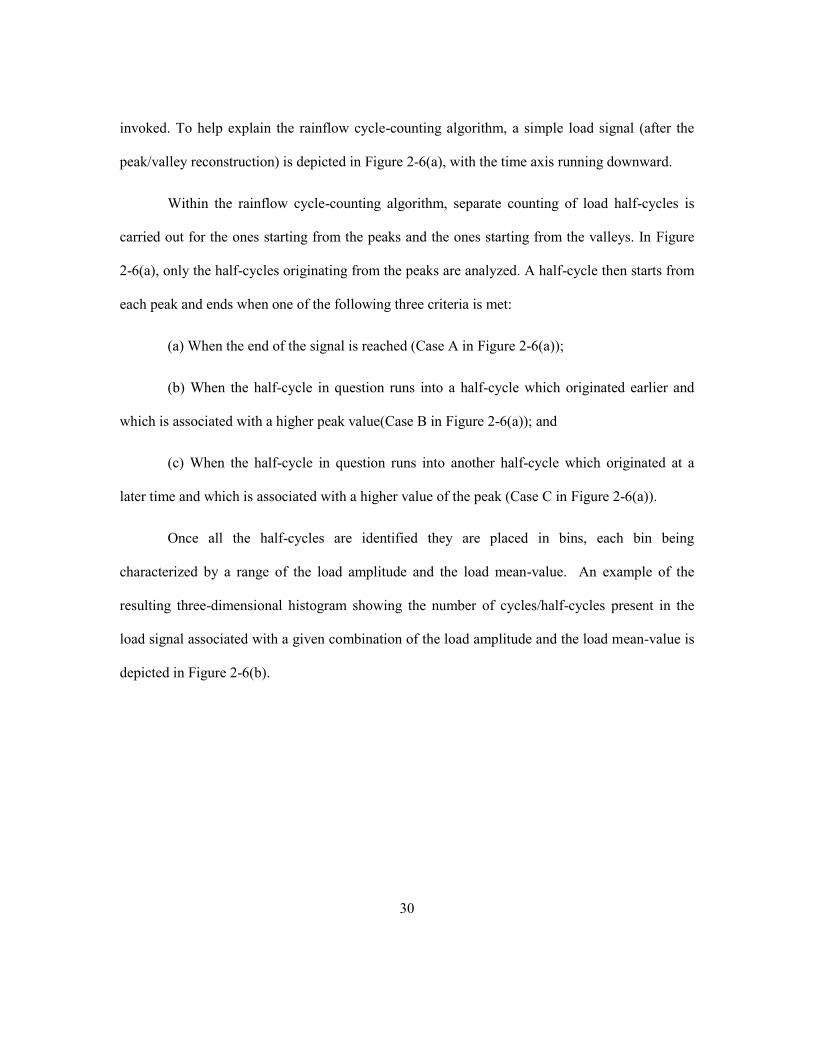
invoked. To help explain the rainflow cycle-counting algorithm, a simple load signal (after the
peak/valley reconstruction) is depicted in Figure 2-6(a), with the time axis running downward.
Within the rainflow cycle-counting algorithm, separate counting of load half-cycles is
carried out for the ones starting from the peaks and the ones starting from the valleys. In Figure
2-6(a), only the half-cycles originating from the peaks are analyzed. A half-cycle then starts from
each peak and ends when one of the following three criteria is met:
(a) When the end of the signal is reached (Case A in Figure 2-6(a));
(b) When the half-cycle in question runs into a half-cycle which originated earlier and
which is associated with a higher peak value(Case B in Figure 2-6(a)); and
(c) When the half-cycle in question runs into another half-cycle which originated at a
later time and which is associated with a higher value of the peak (Case C in Figure 2-6(a)).
Once all the half-cycles are identified they are placed in bins, each bin being
characterized by a range of the load amplitude and the load mean-value. An example of the
resulting three-dimensional histogram showing the number of cycles/half-cycles present in the
load signal associated with a given combination of the load amplitude and the load mean-value is
depicted in Figure 2-6(b).

31
Figure 2-6 (a) Application of the rainflow cycle-counting algorithm to a simple load signal after the
peak/valley reconstruction. Please see text for explanation; and (b) the resulting three dimensional
histogram showing the number of cycles / half-cycles in each mean stress/strain – stress/strain
amplitude bin.
A
A
B
B
C
C (a)
(b) Strain-Amplitude, %
Mean Strain,
%
log
10 (
Nu
mb
er o
f C
ycl
es)

32
Goodman Diagram
Before presenting the basics of the Goodman diagram, it is important to recognize that
fatigue life of a material is a function of both the stress/strain amplitude and the stress/strain mean
value. Often, the stress/strain mean values are quantified in terms of an R-ratio which is a ratio of
the algebraically minimum and the algebraically maximum stress/strain values (associated with
the constant-amplitude cyclic-loading tests). From the definition of the mean stress/strain, it can
be readily shown that fatigue-loading tests carried out under constant R–ratio conditions,
correspond to the tests in which the mean stress/strain scales with the corresponding amplitude.
To construct the Goodman diagram, constant–R/constant-amplitude fatigue-test results are
plotted, in a stress/strain amplitude vs. stress/strain mean-value diagram. As depicted, in Figure
2-7, constant-R data fall onto a line emanating from the origin. In Figure 2-7, R=0.1 and R=0.5
data are associated with a positive/tensile mean stress/strain value, R=-1 corresponds to a zero
mean-value, while R=10 and R=2 pertain to a negative/compressive mean-value.

33
Figure 2-7 An example of the Goodman diagram showing constant fatigue-life data (dashed lines)
and constant R-ratio data (the solid lines emanating from the origin).

34
To construct the corresponding linearized Goodman diagram, constant fatigue-life data
associated with different R–ratio values are connected using straight lines. To complete the
construction of the Goodman diagram, the constant fatigue-life lines are connected to the ultimate
tensile stress/strain and to the ultimate compressive stress/strain points located on the zero-
amplitude horizontal axis. The completed Goodman diagram displayed in Figure 2-7 then
enables, through interpolation, determination of the fatigue life for any combination of the
stress/strain amplitude and stress/strain mean-value. Hence, a three-dimensional histogram
similar to that one shown in Figure 2-6(b) can be constructed except that the number of cycles
here represents the total number of cycles to failure rather than the number of cycles in the
analyzed load-signal. An example of such three-dimensional histogram is displayed in Figure 2-8.

35
Figure 2-8 An example of the three-dimensional histogram showing the effect of stress/strain
amplitude and the stress/strain mean-value of the material fatigue life.
Mean Strain, %
Strain
Amplitude, %
log
10 (
Cy
cles
to
fail
ure
)

36
Miner’s Rule
The cycle counting procedure described earlier enables computation of the number of
cycles/half-cycles in the given load signal which fall into bins of a three dimensional histogram,
Figure 2-6(b). The use of the Goodman diagram, on the other hand, enables the computation of a
similar tri-dimensional histogram but for the number of cycles to failure (i.e. the fatigue life),
Figure 2-8. According to the Miner’s rule, a ratio of the number of cycles and the corresponding
total number of cycles, for a given combination of the stress/strain amplitude and stress/strain
mean-value, defines a fractional damage associated with this component of the loading. The total
damage is then obtained by summing the fractional damages over all combinations of the
stress/strain amplitude and the stress/strain mean-value.
The total fatigue life under the given non-constant amplitude time-varying loading is
obtained by dividing the load-signal duration by the total fractional damage. This procedure
clearly postulates that fatigue failure corresponds to the condition when the total damage is equal
to unity.

37
2.3.4 Wind-Turbine Blade Material Selection
From simple consideration of basic functional and longevity requirements for a HAWT
blade it can be readily concluded that the main blade material-selection indices must be based on
the following material properties:
(a) A high material stiffness to ensure retention of the optimal aero-dynamic shape by the
blade while subjected to strong-wind loading conditions;
(b) A low mass density to minimize gravity-based loading; and
(c) A large, high-cycle fatigue strength to ensure the required 20-year life cycle with high
reliability.
As mentioned earlier, the HAWT-blade is essentially a cantilever beam. If the material
selection methodology proposed by Ashby [11] is utilized, then the first material selection index
can be defined by requiring that the blade attains a minimal mass while meeting the specified
bending-stiffness requirements (or alternatively that the blade attains maximum bending stiffness
at a given mass level). Since the blade mass scales directly with its average cross-sectional area
while its, stiffness scales roughly with the square of its, cross-sectional area, following Ashby’s
material selection procedure one can readily derive the following “light, stiff beam” material
selection index:
// 21
1 EM (2–2)
where E is the material’s Young’s modulus and is its density.
The use of 1M in the HAWT-blade material selection would normally identify foam-like
materials as potential candidates. In these materials, their low stiffness (as quantified by the value
of their Young’s modulus, E ) is more than compensated by their low value. Consequently,

38
1M takes on a large value in the case of foam materials suggesting their suitability for use in the
HAWT-blade applications. However, foam materials would yield very bulky blades which could
present serious design, manufacturing, installation and operational problems. In addition,
potentially open-cell structure and the associated high water-permeability/moisture-absorption
can disqualify these materials from being used in the HAWT-blade applications. To overcome
these problems, a second material selection index (more precisely, a lower-bound material-
property limit) is proposed which requires that the HAWT-blade materials possess a minimal
level of absolute stiffness, i.e.
EM 2 (2–3)
Typically, the minimal level of the Young’s modulus required for a given-blade material
is in a 15-20GPa range.
The two material selection indices defined above utilize two ( E and ) out of the three
previously identified material properties. Inclusion of the third material property (the fatigue
strength) into a material selection index is, however, quite challenging. The reason is that, as
discussed in the previous section, while the constant-amplitude fatigue strength associated with a
given load mean-value and a given fatigue life can be readily determined HAWT-blade material
selection requires the use of a variable-amplitude fatigue life.
As demonstrated in the previous section, the variable-amplitude fatigue life can be, in
principle, computed for a given combination of the sustained quasi-static and time-varying loads.
However, the procedure which is used in this calculation also entails the knowledge of the
constant-amplitude fatigue data under different mean-value/R-ratio conditions. Since the
generation of such data requires an extensive set of experimental tests, these data are not always
available (in particular, in the open literature). Hence, the HAWT-blade material–selection

39
procedure used in the present work had to rely on more readily available material properties.
Specifically, the endurance limit (i.e. the infinite-life constant-amplitude fatigue strength (under a
zero mean loading, i.e., R=-1) will be used in the HAWT-blade material selection. Since
materials with higher fracture toughness will fail in a more gradual manner (enabling a longer life
of the blade between the time of initiation of the first cracks to the final failure). In this way,
blades which have suffered fatigue-induced damage can be identified during periodic inspections
and replaced, preventing more serious consequences, which may result from their unexpected
catastrophic failure while in service.
Based on the discussion presented above, the third and the final HAWT-blade material
selection index can be defined as:
M3 = end ∙ GIc (2–4)
where, end is the endurance limit and GIc the mode-I fracture toughness.
Clearly, the higher is the value of each of the three aforementioned material indices, the
more suited is a given material for use in the HAWT-blade applications.

40
2.4. Results and Discussion
As discussed in Section 2.3, as part of the present work, a computer program was
developed which enables automated creation of fully parameterized geometrical and meshed
models, as well as the generation of a complete finite-element input deck for a large single
composite-laminate 1MW HAWT blade. For a given choice of the airfoil shape, down-the-length
taper and blade twist-angle, the program enables the user to specify lateral location of the shear
webs, thickness for all aerodynamic (i.e. the outer skins) and structural (i.e. the shear webs, the
spar caps, the adhesive layers) component thicknesses and composite- laminate ply stacking for
each component as a whole or for different portions of the same component. In addition,
interfacing of the model-generation computer program with an aerodynamics analysis computer
program [5] enabled automated generation of the sustained wind-based loading conditions. This
was complimented by the addition of non-constant amplitude reference time-varying loading to
construct fairly realistic in-service loading conditions experienced by a large composite-laminate
HAWT blade. The results obtained from the quasi-static finite element analyses of the HAWT-
blade enabled not only investigation of the structural response of the blade (i.e. the extent of the
blade tip deflection, the extent of blade-tip rotation due to bending-to-torsion coupling aero-
elastic effects, etc.), but also predictions of the HAWT-blade high-cycle fatigue controlled life
cycle.
Due to space limitations, only few representative results obtained in the present
investigation will be shown and discussed in the following sections. This will be followed by a
presentation of the results pertaining to the HAWT-blade material selection.
It should be noted that each portion of the present work included a mesh-convergence
study to ensure that the finite-element mesh used was a good compromise between a

41
computational accuracy and computational cost. The results of the mesh convergence studies will
not be shown for brevity.

42
2.4.1 The Baseline Case
At the beginning of the present investigation, a baseline case was first
established/constructed, which is representative of the current commercial 1MW HAWT-blade
designs. In the base-line case which is based on the S818 airfoil-shape [15], Figure 2-9(a), the
primary structural member is a box-shape spar with (vertical) shear webs being located at
distances equal to 15% and 50% of the section-chord length (as measured from the leading edge)
and a substantial build-up in the spar cap thickness between the two vertical shear-webs.
Examination of the HAWT-blade construction depicted in Figure 2-9(a) suggests that due to a
relatively large spar-cap width and laminate thickness, good edge-wise bending stiffness/strength
is expected. This is however, attained at the expense of the flat-wise bending stiffness/strength
which could have been increased should the shaft portion of the shear web had been placed in the
section of the blade associated with the largest blade thickness.
A typical planform, Figure 2-9(b), is assigned to the blade. The plan-form shows the
variation of the blade chord-length with a radial distance r from the hub rotation axis with R
being the radial location of the blade tip. Figure 2-9(b) shows that there is a linear taper from the
maximum-chord section located at r/R=0.25 to the blade tip (r/R=1.0). The blade root is located
at r/R=0.05 and is circular in cross section. The cross section is assumed to remain circular up to
r/R=0.07 and thereafter undergoes a gradual transition to the pure airfoil section located at
r/R=0.25.

43
Figure 2-9 Baseline case of the HAWT blade analyzed in the present work: (a) the airfoil cross
section; and (b) the planform.
(a) Outer-skin
Leading edge Trailing edge
Spar-cap Adhesive
Shear-web
Root Trailing edge
Leading edge
Blade-tip
Maximum-chord (First
Airfoil Location)
(b)

44
As mentioned earlier, HAWT-blades are commonly twisted. Consequently, the baseline-
blade case analyzed here was given a twist along its length. Specifically, the airfoil sections
located at r/R=0.25, 0.5, 0.75 and 1.0 were twisted by 100, 2.5
0, 0
0, and -0.5
0, respectively.
The exterior airfoil skins and the interior vertical shear webs are constructed using a
sandwich-like material consisting of (-450/0
0/45
0) tri-axial fiber-glass composite-laminate face-
sheets separated by a balsa-wood core. The spar caps are constructed of alternating equal-
thickness layers of the tri-axial laminates (described above) and unidirectional laminates making
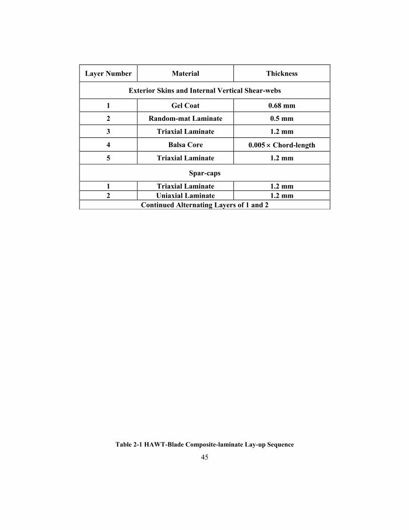
the contribution of 00 laminate and the off-axis laminate 70% and 30%, respectively. A summary
of the composite-laminate lay-up sequences and ply thicknesses used in different sections of the
baseline HAWT-blade design is provided in Table 2-1.
As mentioned earlier, all composite laminates mentioned above were based on epoxy
matrix reinforced with E-glass fibers. As far as the adhesive layers connecting the spar caps to the
interior faces of the skins are concerned, they were taken to be epoxy based. A summary of the
stiffness, mass and composite mixture properties (where applicable) of the materials used are
provided in Table 2-2. In Table 2-2, Tri, Uni and Mix are used to denote respectively the tri-axial,
uni-axial and the spar-cap mixture composite laminates.
45
Table 2-1 HAWT-Blade Composite-laminate Lay-up Sequence
Layer Number Material Thickness
Exterior Skins and Internal Vertical Shear-webs
1 Gel Coat 0.68 mm
2 Random-mat Laminate 0.5 mm
3 Triaxial Laminate 1.2 mm
4 Balsa Core 0.005 Chord-length
5 Triaxial Laminate 1.2 mm
Spar-caps
1 Triaxial Laminate 1.2 mm
2 Uniaxial Laminate 1.2 mm
Continued Alternating Layers of 1 and 2

46
Table 2-2 Summary of the HAWT-Blade Material Properties
Property Uni Tri Mix Random
Mat Balsa
Gel
Coat
Epoxy
Adhesive
Axial Young’s Modulus, Exx
(GPa) 31.0 24.2 27.1 9.65 2.07 3.44 2.76
Transverse Young’s Modulus, Eyy (GPa)
7.59 8.97 8.35 9.65 2.07 3.44 2.76
In-plane Shear Modulus, Gxy (GPa)
3.52 4.97 4.70 3.86 0.14 1.38 1.10
Poisson’s Ratio,xy 0.31 0.39 0.37 0.30 0.22 0.3 0.3
Fiber Volume Fraction, vf 0.40 0.40 0.40 – N/A N/A N/A
Fiber Weight Fraction wf 0.61 0.61 0.61 – N/A N/A N/A
Density,(g/cm3) 1.70 1.70 1.70 1.67 0.l44 1.23 1.15

47
Structural Response of the Baseline HAWT Blade
A set of examples of the results pertaining to the structural responses of the baseline
HAWT-blade is displayed in Figure 2-10(a), 11, 12(a) and 13. These results pertain to the case
when the blade is in the horizontal position; it is fixed at its root and subjected to the gravity
loading, centrifugal forces along its length and the aerodynamic forces resulting from pressure
difference across the blade thickness under the gust-based loads.
In Figure 2-10(a), a spatial-distribution plot of the baseline HAWT-blade external-skin
displacement magnitudes is displayed. The results displayed in this figure reflect mainly the
intrinsic edge-wise bending stiffness of the blade which is important for the overall wind turbine
performance with respect to the ability of the blade to: (a) pass the tower with a required
clearance and (b) impart the appropriate basic structural-dynamics characteristics to the HAWT-
rotor and to the wind turbine, as a whole. It should be noted that an inset is provided in Figure
2-10(a) in order to display the outer-skin composite-laminate lay-up used in the baseline HAWT-
blade design.

48
Figure 2-10 Displacement magnitude distribution over the HAWT blade outer skin caused by a
70m/s gust: (a) the baseline case; and (b) a modified-design case.
Deformed HAWT Blade
Undeformed HAWT Blade
Outer-skin Composite Lay-up
(a)
Gel Coat
Random Mat
Tri-axial Laminate
Balsa Core
Tri-axial Laminate
Undeformed HAWT Blade
(b)
Gel Coat
Random Mat
Tri-axial Laminate
Tri-axial Laminate
Balsa Core
Outer-skin Composite Lay-up
Deformed HAWT Blade

49
A change in the base-line HAWT-blade thickness as a function of normalized distance
from the blade root is displayed in Figure 2-11 (the curve labeled the “Baseline Design” case).
This change is a relative measure of the “flap-wise” stiffness of the blade.

50
Figure 2-11 Variation of the gust-induced HAWT-blade thickness for the blade designs analyzed in
the present work.

51
In Figure 2-12(a), a spatial-distribution plot of the von Mises equivalent stress over the
interior box-shaped beam/spar is displayed. As mentioned earlier, the longitudinal spar is the key
structural member of the blade and any compromise in its structural integrity implies an imminent
loss of the HAWT-blade functionality and its structural failure. Before one can proceed with
assessment of the HAWT-blade safety factor under the imposed gust-based loading conditions,
one must recognize that the effective strength of the blade material may be reduced with respect
to the nominally same material, but a material which is fabricated under normal material
processing conditions and subjected to normal storage/handling practices.

52
Figure 2-12 Von Mises equivalent stress distribution over the HAWT interior structural members
(spar-cap and shear-webs) caused by a 70m/s gust: (a) the baseline case; and (b) a modified-design
case.
Fatigue-Life
Controlling
Elements
(a)
Fatigue-Life
Controlling
Elements
(b)

53
In comparison to the standard materials-processing practice, the material in the HAWT-
blade is generally fabricated under different conditions (i.e. the material is laid-up at the time
when the blade is being manufactured) and is exposed to varying temperatures, ultraviolet-
radiation, humidity, salinity, and other environmental conditions (and is, hence, prone to
accelerated aging/degradation). To account for all these strength-degrading effects, the IFC
61400-1 standard [13] prescribes a set of so-called “material partial safety” factors. Following the
procedure described in Ref. [12], the overall/cumulative material strength-reduction factor was
assessed as 2.9. Hence for the prototypical 500MPa longitudinal strength (before it is corrected
using the material partial safety factors) for the E-glass/epoxy composites used in the present
work, the smallest safety factor (defined as a ratio of the corrected material strength and the
maximum von Mises stresses in the blade = 110.4MPa) is estimated as (500MPa/2.9)/110.4MPa
= 1.57.
In Figure 2-13 (the curve labeled the “Baseline Design” case), a variation of the gust-
induced twist angle in the blade is plotted as a function of the normalized distance from the blade
root. As discussed earlier, bending-to-torsion aero-elastic effects which are responsible for the
observed gust-induced blade tip twist may play a significant role in the overall blade aerodynamic
efficiency and in the passive control of the blade pitch (critical for self-protection of the blades
structural integrity under excessive wind induced loads).

54
Figure 2-13 Variation of the gust-induced HAWT-blade twist angle for the blade designs analyzed in
the present work.

55
Fatigue Life of the Baseline HAWT Blade
As mentioned earlier, the so-called “proportional loading” case was adopted in the
present work according to which stresses scale directly with the load magnitude and the
orientation of their principal components remains unchanged with a change in the load
magnitude. Hence, the stress state in the blade at any instant can be calculated by simply scaling
the quasi-static stress results obtained in previous section (e.g. Figure 2-12(a)), with the
instantaneous wind-based load magnitude. However, before the fatigue life assessment procedure
based on the rain flow cycle counting algorithm, the Goodman diagram and the Miner’s rule can
be applied, the issue of multi-dimensional stress state within different components of the HAWT-
blade has to be addressed. While in metallic materials compressive component(s) of the time-
varying stresses are not generally harmful, composite materials (due to the potential for fiber
micro-buckling) are generally quite susceptible to in-place compressive stresses. To provide a
fairly conservative assessment of the baseline HAWT-blade fatigue life and take into account the
effect of compressive stresses, the stress multi-axiality is handled through the use of a “signed”
von Mises equivalent stress. That is, the entire stress state is assumed to be quantified by the von
Mises equivalent stress to which a sign is attached consistent with the sign of the largest (by
magnitude) principal stress.
As mentioned earlier, time varying component of the wind-induced loading is modeled
by the WISPER load signal. While scaling this load signal (whose values range between 1 and 64
with the level of 25 corresponding to a zero load), the WISPER mean value was assumed to
correspond to the previously computed wind mean speed of 7.6 m/s.
When the procedure outlined in Section 2.3.3 was applied, the fatigue life of the baseline
HAWT-blade was estimated as 32.8years. In Figure 2-12(a), the elements which control the

56
fatigue life of the blade are identified. As could have been expected, these elements are located in
the airfoil/root transition region which is subjected to the highest in-service loads.

57
2.4.2 HAWT-Blade Design Modifications
The geometrical-/meshed-model generator program and the structural and fatigue life
assessment analyses developed in the present work are at a level that they can be readily
incorporated into a design-optimization algorithm. This will be done in our future communication
and the same design-optimization methodology as presented in our recent work [14] will be used.
In this section, however, a couple of examples will be shown in order to demonstrate how few
minor changes in the HAWT-blade design and composite/laminate lay-up can have significant
changes to the blade response/functionality.
In Figure 2-10(b), a plot is shown of the spatial distribution of displacement magnitude
over the HAWT-blade surface. In comparison to the baseline HAWT-blade design, Figure
2-10(a), the design associated with the results displayed in Figure 2-10(b) corresponds to
repositioning of the right shear web from x/c=0.5 to x/c=0.45. Also, the composite-laminate lay-
up used in the modified design case was changed by increasing the balsa core thickness by 15%
relative to the baseline case. The new composite-laminate lay-up is displayed as an inset, in
Figure 2-10(b).
A comparison of the results displayed in Figure 2-10(a) and 2–10(b) shows that edge-
wise stiffness of the HAWT-blade, as measured by its tip-displacement, is a fairly sensitive
function of the lateral position of the right shear web.
A change in the modified-design HAWT-blade thickness as a function of the normalized
distance from the blade root is displayed in Figure 2-11 (the curve labeled “Modified Design”). A
comparison of the results displayed in this figure for the two HAWT-blade designs analyzed
indicates that repositioning of the right shear-web has measurably compromised flap-wise
bending stiffness of the blade.

58
In Figure 2-12(b), a spatial-distribution plot of the von Mises stress over the interior spar
is displayed for the same HAWT-blade design as that used to generate the results displayed in
Figure 2-10(b). A comparison between the results displayed in Figure 2-12(a) and 12(b) shows
that the stresses are somewhat higher in the modified blade design. Consequently, the safety
factor obtained using the same procedure as in the baseline case was found to be reduced from
1.57 to 1.52. Combining this finding with that made in conjunction with Figure 2-10(a)-(b) and
11 suggests that there is a need for the use of design-optimization technique to identify the blade
design with an optimal combination of its functional-performance measures.
The effect of a change in the shear-web/spar-cap composite-laminate lay-up relative to
that used in the baseline case on the extent of bending-to-torsion coupling of the HAWT-blade is
shown in Figure 2-13 (the curve labeled the “Modified Design” case). In this figure, a variation of
the gust-induced twist angle along the length of the blade is displayed. A comparison of the two
sets of results displayed in Figure 2-13 shows that significant changes in the extent of bending-
to- torsion coupling are feasible through modifications in the composite-laminate layup.
The fatigue-life assessment procedure based on the use of the rainflow cycle-counting
algorithm, the Goodman diagram and the Miner’s rule yielded a fatigue life of 27.4 years for the
HAWT-blade design used to generate the results displayed in Figure 2-10(b) and 12(b). Again, it
is clear that both the blade-performance and longevity are sensitive to the blade design and that
the use of design-optimization methods could be quite beneficial. This aspect of the HAWT-blade
design will be addressed in our future communication.

59
2.4.3 HAWT-Blade Material Selection
In Section 2.3.4, it was discussed that the three most important material properties which
control suitability of a given material for use in the HAWT-blade applications are the density, the
Young’s modulus and the fatigue strength/life. Three related material-selection indices were also
derived and it was argued that one of them, i.e. index M2, Eq. (2–3), is essentially a material-
property limit index which is used to screen out the materials which do not possess the sufficient
level of stiffness, as quantified by their Young’s modulus. Consequently, the condition
M2≥20GPa was applied at the onset of the present material selection process to eliminate
unacceptable materials. Then, indices M1 and M3 are used to carry out the HAWT-blade material
selection in accordance with the procedure outlined in Section 2.3.4. In constructing the
corresponding material-selection charts various open-literature material-data sources were
consulted. The Young's modulus data used pertain to the mean in-plane value of this quantity.
The results of the material selection procedure carried out in the present work are summarized in
Figure 2-14(a)-(c). It should be noted that, for clarity, materials appearing in Figure 2-14(a)-(c)
are labeled using numbers and a legend is provided in Figure 2-14(d) for the number labels used.
In Figure 2-14(a), the Young’s modulus vs. density data are compiled for a number of
thermosetting polymer matrix composites. A log-log plot was used in Figure 2-14(a) and three
lines with a constant slope were drawn in accordance with the definition of the first material
selection index, M1, Eq. (2–2). The three guide-lines (with a slope of 2.0) are associated with the
M1-levels of 10,500, 22,500 and 40,000 GPa0.5
/(kg/m3) with the larger M1 value causing the
guide-line to be shifted upward. Also, a 20GPa dashed guide-line is displayed in Figure 2-14(a) in
order to denote the previously-established lower-bound for the Young’s modulus of the candidate

60
materials for use in the HAWT-blade applications. With respect to the M1 material selection
index alone, the optimal materials are those located above the topmost guide-line.
In Figure 2-14(b), a linear-linear plot is shown of the data pertaining to the endurance
limit (x-axis) and the toughness (y-axis) for the same set of materials as that used in Figure
2-14(a). Three solid guide-lines are also shown in Figure 2-14(b) and they correspond to the M3-
levels of 1, 7 and 13 MPa2∙m. Again, with respect to the M3 material selection index alone, the
optimal materials are those located above the topmost guide-line.
Since different material are identified as optimal if material selection is based on the use
of a single index (M1 or M3), Figure 2-14(a)-(b), a procedure was developed here which takes into
account both of these material indices in the HAWT-blade material-selection process. A linear-
linear plot of M3 vs. M1 material selection indices (normalized by the values of these two indices
in a commonly used HAWT- blade material, i.e., an E-glass uni-directionally-reinforced epoxy–
matrix composite) is shown in Figure 2-14(c). The three solid lines displayed in Figure 2-14(c)
correspond to the values of 2, 5 and 10 for a combined material selection index, M, defined as:
M = wM1 + (1-w)M3 (2–5)
where the weighting factor w for the material selection index M1 is set 0.5, making the weighting
factor for the mutual selection index M3 also equal 1.0-0.5=0.5.
Simple examination of the results displayed in Figure 2-14(c) reveals that, for the most
part, carbon-fiber reinforced PEEK-(Poly-ether-ether-ketone) or polyimide-matrix composites are
favored. In the case of E-glass fiber reinforced composites, a phenolic matrix appears to be
preferred over the traditionally used epoxy or poly-ester. The main reason for the carbon fibers
outperforming the E-glass fibers is their higher density-normalized stiffness, while the emergence
of the phenolic polymers appears to be related to higher toughness levels imparted to the

61
composite material by this polymeric matrix. The main reason for the currently preferred HAWT-
blade material, i.e. E-glass fiber reinforced epoxy–matrix composites, is the relatively low
material cost combined with the overall good structural/fatigue-life performance.

62
Figure 2-14 Material property charts used in the HAWT-blade material selection process. Please see
text for details.
MM33==1133MMPPaa22..
mm
MM33==11MMPPaa22..
mm
MM33==77MMPPaa22..
mm
20
19
24
9 3 23
8 7
13 11
5
(b)
(a)
5
3
8
19
7
23
9 24 11
20
13
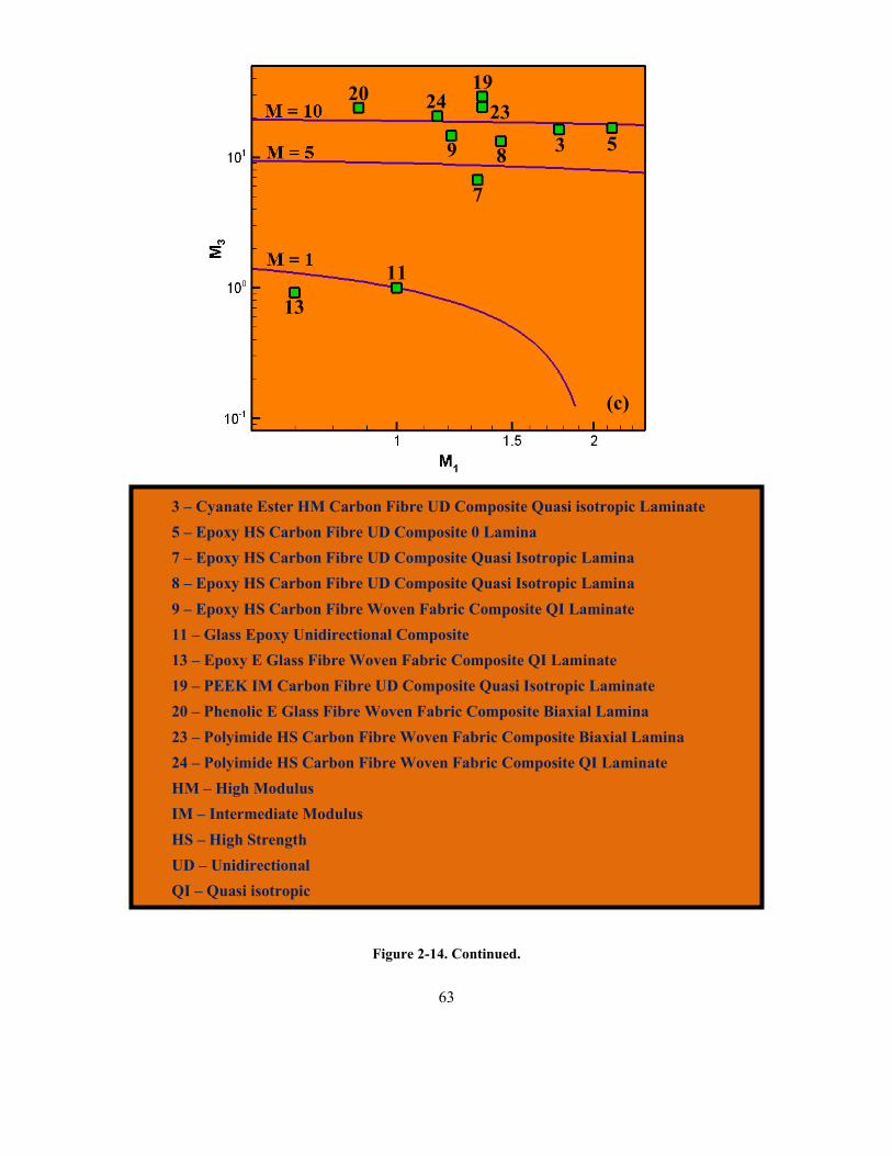
63
Figure 2-14. Continued.
3 – Cyanate Ester HM Carbon Fibre UD Composite Quasi isotropic Laminate
5 – Epoxy HS Carbon Fibre UD Composite 0 Lamina
7 – Epoxy HS Carbon Fibre UD Composite Quasi Isotropic Lamina
8 – Epoxy HS Carbon Fibre UD Composite Quasi Isotropic Lamina
9 – Epoxy HS Carbon Fibre Woven Fabric Composite QI Laminate
11 – Glass Epoxy Unidirectional Composite
13 – Epoxy E Glass Fibre Woven Fabric Composite QI Laminate
19 – PEEK IM Carbon Fibre UD Composite Quasi Isotropic Laminate
20 – Phenolic E Glass Fibre Woven Fabric Composite Biaxial Lamina
23 – Polyimide HS Carbon Fibre Woven Fabric Composite Biaxial Lamina
24 – Polyimide HS Carbon Fibre Woven Fabric Composite QI Laminate
HM – High Modulus
IM – Intermediate Modulus
HS – High Strength
UD – Unidirectional
QI – Quasi isotropic
11
8
19
9
20 24 23
3 5
7
13
(c)

64
It should be noted that the material-selection procedure employed in the present work is
based on the use of stereotypical material properties of the common thermosetting-polymer
matrix composite plies/laminae reinforced with either uni-directional or cross-woven fiber mats.
Consequently, the procedure does not include the full effect of composite-laminate architecture.
That is, properties of the composite laminates are derived not only from those of the associated
laminae but can be tailored over relatively large range by varying plies thickness and orientation,
stacking sequence as well as by hybridization of the laminate. Laminate hybridization can be
carried out on the ply scale (by combining fibers of different types, e.g. by combining glass and
carbon fibers within the single laminae) or on the laminate scale (by stacking plies with different
fiber reinforcements, e.g., by alternate stacking of the glass-fiber reinforced plies and the carbon-
fiber reinforced plies). It should be noted that ply-level hybridized laminae can be readily
included in the present material selection procedure once the appropriate material properties
become available. On the other hand, the effect of laminate-level hybridization can be readily
included through the ply-stacking optimization procedure mentioned in Section 2.4.2.

65
2.5. Summary and Conclusions
Based on the results obtained in this portion of the work, the following main summary
remarks and conclusions can be drawn:
1. A fully parameterized computer program has been developed for automated generation
of the geometrical and finite-element meshed models of the Horizontal Axis Wind Turbine
(HAWT) blades. The program enables the specification of the basic blade geometrical and
structural parameters (e.g., airfoil shape, size and lateral location of the longitudinal spar/beam,
thickness of the adhesive layers joining the beam to the external blade skins, etc.) as well as the
basic and locally different composite-laminate architecture and lay-up sequence.
2. Fairly realistic, yet generic wind-based (sustained and time-varying) loading conditions
are compiled and applied to a stereotypical 1MW HAWT-blade in order to assess its structural
response as well as to assess its longevity.
3. A preliminary parameter variation study was conducted which revealed that further
improvements in the HAWT-blade performance are possible with targeted changes in the blade
geometry and the composite-laminate lay-up.
4. A simple HAWT-blade material selection procedure was developed which combines
weighted contributions of the material indices pertaining to the blade performance and longevity.
The results revealed that, as expected, from the performance point of view carbon-fiber
reinforced composites are preferred over the traditionally-used E-glass fibers reinforced
composites and that epoxy may not be best choice for the composite-material matrix.

66
2.6. References
1. “20% Wind Energy by 2030, Increasing Wind Energy’s Contribution to U.S. Electricity
Supply,” DOE/GO-102008-2567, July 2008, http://www.osti.gov/bridge
2. T. Burton, D. Sharpe, N. Jenkins, E. Bossanyi, “Wind Energy Handbook,” John Wiley &
Sons Ltd, 2001.
3. M. Selig, “UIUC Airfoil Coordinates Database – Version 2.0,”
http://www.ae.uiuc.edu/mselig/ads/coord_database.html, 2006.
4. MATLAB, The Language of Technical Computing, 7th Edition, 2006 (The MathWorks Inc.,
MA.
5. M. Hepperle, “JavaFoil Users Manual,” http://www.mh-aerotools.de/airfoils/javafoil.htm,
2005.
6. A. A. Ten Have, “WISPER and WISPERX: Final Definition of Two Standardized Fatigue
Loading Sequences for Wind Turbine Blades,” NLR-TP-91476U, National Aerospace
Laboratory NLR, Amsterdam, the Netherlands, 1992.
7. ABAQUS/Standard Version 6.8-1, User Documentation, Dassault Systemes, 2008.
8. M. Matsuiski, T. Endo, “Fatigue of metals subjected to varying stress”, Japan Soc. Mech.
Eng, 1969.
9. J. Goodman, “Mechanics Applied to Engineering,” London: Longman, Green, & Co., 1899.
10. M. A. Miner, “Cumulative damage in fatigue,” J. Appl. Mech, 12:A159–64, 1945.
11. M. F. Ashby, “Materials Selection in Mechanical Design,” Third Edition, Elsevier
Butterworth Heinemann, 2005.
12. D. A. Griffin, “WindPact Turbine Design Scaling Studies Technical Area-1-Composite
Blades for 80- to 120-Meter Rotor”, NREL, Washington, 2001.
13. IEC-61400-3 (2009-02) Wind turbines - Part 3: “Design requirements for offshore wind
turbines Maintenance Result Date”: p 201
14. M. Grujicic, G. Arakere, W. C. Bell, H. Marvi, H. V. Yalavarthy, B. Pandurangan, I. Haque
and G. M. Fadel, “Reliability-based Design Optimization for Durability of Ground-vehicle
Suspension-system Components,” Journal of Materials Engineering and Performance, 19, 3,
pp. 301–313, 2010.
15. D. M. Somers, “The S816, S817 and S818 Airfoils”, NREL, Pennsylvania, 1992.
16. http://www.siemens.com/press/en/presspicture/index.php?view=list&content=&tag=EWP201
309062, accessed May 6, 2014.

67
CHAPTER 3: HORIZONTAL–AXIS WIND–TURBINE: GEAR–BOX FAILURE VIA
TOOTH–BENDING FATIGUE
3.1. Abstract
Wind energy is one of the most promising and the fastest growing alternative-energy
production technologies which have been developed in response to stricter environmental
regulations, the depletion of fossil-fuel reserves, and the world’s ever-growing energy needs. This
form of alternative energy is projected to provide 20% of the US energy needs by 2030. For
economic reasons, wind turbines (articulated structures which convert wind energy into electrical
energy) are expected to operate, with only regular maintenance, for at least twenty years.
However, some key wind-turbine components (especially the gearbox) tend to wear down,
malfunction and fail in a significantly shorter time, often three to five years after installation,
causing an increase in the wind-energy cost and in the cost of ownership of the wind turbine.
Clearly, to overcome this problem, a significant increase in long-term gearbox reliability needs to
be achieved. While purely empirical efforts aimed at identifying shortcomings in the current
design of the gearboxes are of critical importance, the use of advanced computational methods
engineering analyses can also be highly beneficial. The present work demonstrates the use of the
finite element analysis in modeling and elucidating the root cause of one of the gear failure modes
(i.e. tooth-bending fatigue) under a variety of normal operating and extreme wind-loading
conditions.

68
3.2. Introduction
The main objective of the present work is to address the problem of long-term reliability
and the modes of failure of gearboxes used in wind (energy-harvesting) turbines. Consequently,
the concepts most relevant to the present work are: (a) wind-energy harvesting; (b) wind-turbine
gearbox reliability; and (c) root causes and main modes of gear damage and failure. In the
remainder of this section, a brief description is provided for each of these concepts.

69
3.2.1 Wind Energy Harvesting
The depletion of fossil-fuel reserves, stricter environmental regulations and the world’s
ever-growing energy needs have led to deployment/ utilization of various alternative/renewable
energy sources, among which wind energy is one of the most promising and the fastest growing
installed alternative-energy production technologies. In fact, it is anticipated that by 2030, at least
20% of the U.S. energy needs will be met by various onshore and offshore wind-farms.
A wind turbine is essentially a converter of wind energy into electrical energy. This
energy conversion is based on the principle of having the wind drive a rotor, thereby transferring
wind power to the electrical generator. To attain greater structural stability of the rotor and a high
value of aerodynamic efficiency, the rotor is usually constructed as a set of three aerodynamically
shaped blades. The blades are (typically) attached to a horizontal hub (which is connected to the
rotor of the electrical generator, via a gearbox/drive–train system, housed within the nacelle). The
rotor/hub/nacelle assembly is placed on a tower and the resulting wind energy converter is
referred to as the Horizontal Axis Wind Turbine (HAWT).
To reduce the energy production cost (typically expressed in $/kW•hr), commercial wind
turbines have grown considerably in size over the last 30 years. The large wind-turbine
economics is based on the fact that as the hub-height/wind-turbine rotor radius increases, the
average wind speed/wind energy captured increases due to the so called “wind shear effect.”
Consequently, for the same energy production level, lesser number of wind turbine units is
required, which in turn leads to a reduction in the cost of operation of the farm. As the size of the
wind turbine rotor increases, the structural performance, durability and dynamic-stability
requirements tend to become more and more challenging to meet.

70
Turbine blades and the gearbox are perhaps the most critical components/subsystems in
the present designs of wind turbines. The present work deals only with the issues related to the
performance, reliability and modes of failure of gearbox components. In our recent work [5, 6],
two-level multi-disciplinary design-optimization methods and tools were developed for
determination of the optimal shape and size of glass-fiber reinforced epoxy-matrix composite
HAWT blades.

71
3.2.2 Wind Turbine Gearbox Reliability
Wind-turbine gearbox failure remains one of the major problems to the wind-energy
industry [14]. The root causes of gearbox failure in the earlier designs are associated with the
problems related to: (a) fundamental design errors; (b) manufacturing deficiencies; and (c) under-
estimation of the operating loads. While these problems have been mainly eliminated over the last
20 years, wind-turbine gearboxes still generally fail to achieve their design life goal of twenty
years. The combination of these high failure rates and the high cost of gearboxes, has contributed
to: (a) increased cost of wind energy; and (b) higher sales price and cost of ownership of wind-
turbines. Clearly, to make wind energy a more viable renewable-energy alternative, the long-term
gearbox reliability must be significantly increased.
The current state of understanding of the basic features and processes/mechanisms related
to the failure of wind-turbine gearboxes can be summarized as follows [14]: (a) gearbox failure
appears to be of a generic character, i.e. not strongly related to the differences in their design; (b)
gearbox failure cannot be generally attributed to poor workmanship; (c) gear failure is frequently
the result of excessive and unexpected (e.g. misalignment) loading conditions. In other cases, the
gearbox failure may be initiated in overloaded bearings, and the resulting bearing debris
propagate to the gears, causing tooth wear and gear misalignment; and (d) the essential features
and mechanisms of gearbox damage and failure appear not to change with size of the wind
turbine.
A labeled schematic of a prototypical wind turbine gearbox is shown in Figure 3-1. The
low-speed stage of the gearbox is a planetary configuration with either spur (the present case) or
helical gears. In this configuration, the planetary-gear carrier is driven by the wind-turbine rotor,

72
the ring gear is stationary/reactionary, while the sun pinion shaft drives the intermediate gearbox
stage, and, in turn, the high-speed stage. Typically, both the intermediate and high-speed stages
are composed of helical gears (the damage and fatigue-failure of which is the subject of the
present manuscript).

73
Figure 3-1 Schematic of a prototypical wind-turbine gearbox. The major components and sub-
systems are identified.
Ring Gear
High-speed
Stage
Intermediate
Stage
Sun Pinion
Low–Speed
Stage
Planetary Gear Helical Gears
Input Shaft
Output
Shaft

74
3.2.3 Main Modes of Gear Damage and Failure
Post-mortem examination of the field wind-turbine gearboxes revealed two main modes
of gear failure [2, 3]:
(a) tooth-bending high-cycle fatigue failure – The defining features of this gear-tooth
failure mode can be summarized as: (i) Fatigue cracks are typically found to be initiated at the
root radii on the engaged (loaded in tension) side of the gear teeth; (ii) Cracks tend to originate
preferentially at the locations associated with the largest principal stresses. Under normal loading
conditions, the highest stresses are typically found at the tooth base, while under abnormal
loading conditions (e.g. in the case of gear misalignment), the location of the highest stresses is
related to the character and extent of loading abnormality; (iii) Crack growth is generally
characterized by an L-shaped trajectory, i.e. the crack, nucleated at the engaged side of the tooth
initially propagates inwards and below the tooth, and then makes a turn outward towards the
opposite side of the same tooth (leading to the tooth breaking off); and (iv) Due to the subsequent
overloading effects, failure of one tooth is often accompanied by failure of adjacent teeth, in rapid
succession; and
(b) surface contact fatigue failure – Depending on the character and spatial distribution
of the stresses at and beneath the contact surfaces, the following three modes of this type of
failure have been identified: (i) Formation of microscopic pits typically associated with rolling-
contact fatigue loading conditions along the pitch-line of gear teeth. These pits mainly affect the
extent and nature of the gear-tooth surface roughness; (ii) Formation of larger-size surface pits
which are typically attributed to a combination of sliding- and rolling-contact fatigue loading
conditions (typically away from the pitch-line, especially in the regions characterized by

75
“negative”-sliding conditions). These pits act as potent stress risers and can facilitate initiation of
other gear-tooth failure mechanisms (e.g. tooth-bending fatigue failure); and (iii) Spallation, i.e.
formation and shedding of large flakes from the contact surfaces. Often, the spall debris is formed
as a result of fracture along the interface between the case-hardened surface layer and the tooth
core.

76
3.2.4 Main Objectives
To respond to the aforementioned problems related to the relatively frequent and costly
failure of wind-turbine gearboxes, wind-turbine manufacturers tend to re-engineer critical
components and include them into new subsystems (gearbox designs). To demonstrate the utility
of the new designs, the re-engineered gearboxes are installed and field testing is started. While
this approach may help address the gearbox reliability concerns, it is associated with long field-
test times and costly post-mortem failure analyses necessary to achieve the desired level of
confidence in the new design. In addition, when the field-test results become available, it is likely
that new wind-turbine, and hence new gearbox designs, will dominate the market, making the
field-test results less valuable.
To overcome the foregoing shortcomings of the purely empirical approach aimed at
addressing the wind-turbine gearbox reliability, the use of advanced computer-aided engineering
methods and tools is advocated in the present work. While such a computational approach is not a
substitute for the aforementioned re-engineer-and-field-test approach, it can provide
complementary insight into the problem of wind-turbine gearbox failure and help gain insight
into the nature of the main cause of this failure. In addition, computational engineering analyses
enable investigation of the gear failure in a relatively short time, under: (a) a variety of wind-
loading conditions comprising both the expected design-load spectrum as well as the unexpected
extreme loading conditions; and (b) conditions in which the transfer of loads (both primary torque
loads and non-torque loads) from the shaft and mounting reactions occurs in a non-linear or
unpredicted manner.

77
Considering the aforementioned potential benefits of the computer-aided engineering
analysis, the main objective of the present work is to carry out a computer-aided engineering
analysis of the tooth-bending high-cycle fatigue-failure of wind-turbine helical gears found in the
intermediate-speed stage of the gearbox. Failure of these gears is often found to be the cause of
the wind-turbine gearbox failure.

78
3.2.5 Chapter Organization
A concise summary of the computational approach used in the investigation of wind-
turbine gearbox gear-bending stress and high-cycle fatigue failure analyses is presented in
Sections 3.3 and 3.4, respectively. The key results yielded by the present investigation are
presented and discussed in Section 3.5, while the main conclusions resulting from the present
work are summarized in Section 3.6.

79
3.3. Finite-Element Stress Analysis
As mentioned earlier, helical-gear tooth-bending high-cycle fatigue-failure is one of the
main modes of failure of wind-turbine gearboxes. Since fatigue-cracks are generally initiated at
surface locations associated with the largest contact (as well as sub-surface) stresses, one must
determine accurately spatial distribution and temporal evolution of the contact (as well as
through-the-volume) stresses, before attempting to assess fatigue strength and service life of
wind-turbine gears. Accurate determination of these stresses is most conveniently carried out
through a finite-element-based analysis. In the present section, details regarding the helical
mating-gear interactions during the transfer of wind-turbine torque loads and the finite-element
modeling and analysis procedure employed are presented.

80
3.3.1 Problem Formulation
The basic problem analyzed here involves the structural response of two mating wind-
turbine helical gears located within the intermediate stage of the gearbox, during the transfer of
the torque loads under different expected and abnormal wind-loading conditions. The results to be
obtained will subsequently be used to assess tooth-bending high-cycle-fatigue failure-strength and
service-life of the subject helical gears under imposed wind-loading conditions.

81
3.3.2 Computational Analysis
The finite-element analysis (FEA) used here is an adaptation of our recent work [7, 10,
12] dealing with the friction stir welding process model. In the remainder of this section, a brief
overview is provided of the key aspects of the employed FEA.
1) Geometrical Model
The geometrical model/computational domain of the problem analyzed in this portion of
the work is depicted in Figure 3-2(a). The model comprises two mating helical gears and their
two associated shafts. Under ideal gear-meshing conditions (i.e. in the absence of gear
misalignment), the axes of the two shafts are parallel and aligned in the global Cartesian y-
direction, as indicated in Figure 3-2(a). On the other hand, under abnormal loading conditions
involving gear misalignment, the axes of the two shafts are assumed not to be parallel.
2) Meshed Model
Each of the four components (i.e. two helical gears and two shafts) is meshed using four-
node, first-order, reduced-integration, tetrahedral continuum elements. After conducting a mesh-
sensitivity analysis to ensure that further refinement in the mesh size does not significantly affect
the results (not shown for brevity), a meshed model containing ca. 460,000 tetrahedron elements
(of comparable size and shape) was adopted for the analysis. A close-up of the meshed model
used in this portion of the work is depicted in Figure 3-2(b).

82
Figure 3-2 (a) Geometrical model; and (b) Close-up of the meshed model consisting of two helical
gears and two shafts, used in the present work.
(a)
(b)

83
3) Computational Algorithm
Due All calculations are based on a transient, displacement-based, purely Lagrangian,
conditionally-stable, explicit finite-element algorithm. Before the analysis is initiated, the two-
gear-shaft assembly is assumed to be stationary and subject only to the gravity-induced stresses.
Then, at the beginning of the analysis, the rotational speed of the shaft associated with the larger
(driving) helical gear is ramped up to its final value by ensuring that: (a) the two gears are
engaged; (b) the shaft of the smaller (driven) helical gear is allowed to rotate about its axis; and
(c) a prescribed torque load is transmitted through engagement, and subsequent meshing of the
gears. It should be noted that the shafts and their respective gears are connected so that the
rotation of a shaft implies rotation of the associated gear and vice versa.
4) Initial Conditions
As mentioned above, the two-gear/shaft assembly is initially assumed to be stationary
and only the stresses associated with gravity-loading are assumed to be present within each
component.
5) Boundary Conditions
The following boundary conditions were utilized: (a) the center points of the shaft end-
faces (treated as rigid surfaces) are prevented from undergoing translation; (b) rotational speed is
prescribed to one of the end-faces of the driving shaft (i.e. the shaft associated with the larger
helical gear); and (c) a constant opposing torque is applied to one of the end-faces of the driven
shaft (i.e. the shaft associated with the smaller helical gear).
6) Contact Interactions

84
The gear-gear normal interactions are analyzed using a penalty-contact algorithm. Within
this algorithm, (normal) penetration of the contacting surfaces is resisted by a set of linear springs
which produces a contact pressure that is proportional to the depth of penetration. Typically,
maximum default values, which still ensure computational stability, are assigned to the (penalty)
spring constants. Force equilibrium in a direction collinear with the contact-interface normal then
causes the penetration to acquire an equilibrium (contact-pressure dependent) value. It should be
noted that no contact pressures are developed unless (and until) the nodes on the “slave surface”
contact/penetrate the “master surface”. On the other hand, the magnitude of the contact pressure
that can be developed is unlimited. As far as the tangential gear-gear interactions (responsible for
transmission of the shear stresses across the contact interface) are concerned, they are modeled
using a modified Coulomb friction law. Within this law, the maximum value of the shear stresses
that can be transmitted (before the contacting surfaces begin to slide) is defined by a product of
the contact pressure and a static (before sliding) and a kinetic (during sliding) friction coefficient.
In addition, to account for the potential occurrence of a “sticking condition” (sliding occurs by
shear fracture of the softer of the two materials, rather than by a relative motion at the contact
interface), a maximum value of shear stress (equal to the shear strength of the softer material) that
can be transmitted at any level of the contact pressure is also specified.
As far as the friction coefficient is concerned, it is generally assumed that this contact
parameter is controlled by the formation and shearing of micro-welds (i.e. micron-sized regions at
which contacting surface asperities are bonded). Furthermore, it is recognized that the friction
coefficient is a function of a number of factors such as the contact interface (mean) temperature,
slip speed, contact pressure, contact surfaces’ roughness/topology, etc. To assign the appropriate

85
value to the friction coefficient, functional relationships derived in our recent work [8] were
analyzed.
7) Material Model
The helical-gear and shaft materials are assumed to be of an isotropic (linearly) elastic
and (strain-hardenable) plastic character. Due to the isotropic nature of the material(s) used, the
elastic response is fully defined in terms of two elastic engineering moduli (e.g. the Young’s
modulus, E, and the Poisson’s ratio, ). The plastic response of the material(s) is defined by
specifying the following three functional relations: (a) a yield criterion; (b) a flow rule; and (c) a
constitutive law. These functional relations and their parameterization for the gear and shaft
reference material, AF1410, a secondary-hardening martensitic tool steel, can be found in [9, 11,
12].
8) Computational Tool
The problem of helical gear engagement, meshing and torque-load transfer is executed
using an explicit solution algorithm implemented in ABAQUS/Explicit, a general-purpose finite
element solver [1]. This algorithm was chosen because it is associated with comparatively low
computational cost when dealing with three-dimensional problems dominated by contact (as is
the present case). Since the dynamic, explicit finite-element formulation is only conditionally
stable, care had to be taken to ensure that the time increments during the analysis do not exceed
the critical time increment [4].

86
3.4. Fatigue Strength and Life-Cycle Prediction
In this section, a brief description is provided regarding the post-processing procedures
applied to the results yielded by the finite element analysis (described in the previous section) in
order to assess the fatigue-life of the helical gears used within the intermediate stage of the
gearbox.

87
3.4.1 Fatigue-Crack Initiation
Fatigue-crack initiation is a complex process which is greatly influenced by factors such
as material microstructure, the character and intensity of the applied stress, and on various micro-
and macro-scale geometrical parameters. Since fatigue-crack initiation is often observed to be
associated with the formation of persistent slip bands and plastic-accommodation zones around
grain and twin boundaries, inclusions, etc. [e.g. 13], it is generally treated as a (strain-controlled)
short-cycle fatigue process. In other words, formation of fatigue cracks is assumed to be preceded
by the operation of highly-localized plastic-deformation processes. Furthermore, it is generally
assumed that: (a) fatigue-crack initiation occurs in the region associated with the maximum value
of the largest principal stress; and (b) the transition from the strain-controlled fatigue-crack
initiation stage to the stress-controlled fatigue-crack growth stage occurs at a threshold crack
length, (typically set to a value in the 0.1–0.2 mm range).
Due to its strain-controlled character, the fatigue-crack initiation process is modeled here
by combining:
(a) the conventional Coffin-Manson equation, cifp N2'2' , where 2' p is the
equivalent plastic strain amplitude, f' is the fatigue ductility coefficient, c is the fatigue
ductility exponent, iN is the number of cycles required to reach tha , and iN2 is the
corresponding number of stress reversals; with
(b) the additive decomposition of the total equivalent strain amplitude 2' into its
elastic, 2'e , and plastic components;
(c) fatigue micro-yielding constitutive law, '1'2''2' nffp , where 2' is the

88
equivalent-stress amplitude, 'n is the cyclic strain-hardening exponent and f' is the fatigue
strength coefficient;
(d) Hooke’s law, eE '' , where E is the Young’s modulus and
(e) stress-based fatigue-life relation, bifFL N2''2' , where FL' is the material
fatigue/endurance limit and b is a material parameter.
This procedure yields the following equation:
c
iNfb
iNE
fn
f
FLfE
FL 2'2'
'1
'2
'2''
'2'
2
'
(3–1)
Once the region within a gear associated with the largest value of the maximum principal
stress is identified and the corresponding equivalent stress amplitude computed (using the finite-
element results), Eq. (3–1) can be solved iteratively to get the number of cycles to fatigue-crack
initiation iN for a given combination of gear-material and cyclic loading. To include the effect of
surface condition on the fatigue-crack initiation process, FL' is typically multiplied by a positive
coefficient (smaller than 1.0) which accounts for the effect of initial surface roughness or contact-
fatigue-induced surface damage.

89
3.4.2 Fatigue-Crack Growth
Once the crack reaches its threshold length tha , the fracture process transits into the
fatigue-crack growth regime. Since this regime is stress-controlled, it is modeled here using the
theory of linear elastic fracture mechanics (LEFM). Specifically, fatigue-crack growth is modeled
using the Paris equation, which relates the rate of increase in the sub-critical crack length with an
increase in the loading-cycle number, Na dd , with the (maximum – minimum) applied (generally
mixed-mode) stress-intensity cycling range thKK as:
maKCdN
da (3–2)
where, thK , C and m are material parameters. The maximum number of fatigue-loading cycles
in the crack-growth regime, gN , is obtained by integrating Eq. (3–2) as:
c
th
p a
am
N
aK
da
CdN
Δ
1
0
(3–3)
where, ca is the critical crack length (i.e. the crack length at which unstable fracture is initiated
under static loading conditions). To carry out the integration described by Eq. (3–3), one must
know the functional relationship between the K (i.e. K ) and the current crack length under the
given crack configuration and loading conditions. While closed-form K vs. a functional
relations are available for the cracks of simple geometry and for the simple loading cases, under
more complex crack-geometry/-loading scenarios, this function must be evaluated numerically. In
the present work, the interaction-integral finite-element method [1] is used to determine the
sought-after K vs. a relation. Within this method, the K vs. a relation is obtained by: (a)
introducing an initial crack of length tha at the location yielded by the foregoing crack-initiation
analysis; (b) setting the incremental fracture surface equal to the plane orthogonal to the

90
maximum principal stress; (c) controlling the crack growth by successively prescribing small
crack extensions; (d) evaluating the mixed-mode stress intensity factor as a function of the
associated modes I, II and III stress intensity factors as
2222
1
2IIIIII KKKK
(3–4)
where is the Poisson’s ratio; and (e) repeating the procedure until the computed mixed-mode
stress intensity factor reaches its critical (unstable crack growth) value.

91
3.5. Results and Discussion
In this section, the main results of the finite-element stress analysis and the post-
processing fatigue-crack initiation and growth analyses are presented and discussed. While the
present computational framework enables the generation of results under numerous gear-
material/transfer-torque/gear-misalignment scenarios, due to space limitations, only a few
prototypical results will be presented and discussed.

92
3.5.1 Temporal Evolution/Spatial Distribution of Gear-Tooth Stresses
In this section, a few prototypical finite-element results pertaining to the distribution of
the maximum principal stress over one tooth of the driven helical gear are presented and
discussed in the context of the expected fatigue-life (in particular, the portion of the fatigue-life
related to the crack-nucleation stage).
1) Aligned-Gear Case
Typical temporal evolution and spatial distribution of the maximum principal stress over
the surface of a tooth of the driven gear (for the case of perfectly aligned shafts) are shown in
Figure 3-3(a)–(d). It is seen that as expected, the maximum principal stress displays cyclic
behavior. That is, as the gears rotate, the (unengaged) tooth in question becomes progressively
engaged and subsequently disengaged. Furthermore, examination of the results displayed in
Figure 3-3(a)–(d) reveals that during this process, the location associated with the largest value of
the maximum principal stress changes with the extent of gear rotation. This observation is
important since, as postulated by the fatigue-crack initiation model described in an earlier section,
fatigue-cracks are nucleated (via the operation of plastic micro-yielding phenomena) in the region
associated with the highest value of the maximum principal stress.

93
Figure 3-3 Typical temporal evolution and spatial distribution of the maximum principal stress over
the surface of a tooth of the driven gear (for the case of perfectly aligned shafts).
< 650 MPa > 800 MPa
(a)
> 875 MPa
(b)

94
Figure 3–3 Continued
> 960 MPa
(c)
> 960 MPa
(d)

95
The effect of the torque transferred by the gear-pair analyzed on the largest value of the
maximum principal stress, and on the corresponding value of the von Mises equivalent stress, in
the subject gear-tooth (for the case of perfectly aligned shafts) is shown in Figure 3-4. It is seen
that as the transferred torque increases, both the highest value of the maximum principal stress
and the associated von Mises stress on the surface of the subject gear-tooth also increase
(approximately linearly). This finding then implies, and the results of the fatigue-service-life
analysis (presented below) will confirm, that as the transferred torque increases, the number of
loading cycles required for fatigue-crack nucleation decreases.

96
Figure 3-4 The effect of the torque transferred by the gear-pair analyzed on the largest value of the
maximum principal stress in the subject gear-tooth).
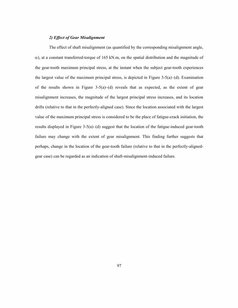
97
2) Effect of Gear Misalignment
The effect of shaft misalignment (as quantified by the corresponding misalignment angle,
), at a constant transferred-torque of 165 kN.m, on the spatial distribution and the magnitude of
the gear-tooth maximum principal stress, at the instant when the subject gear-tooth experiences
the largest value of the maximum principal stress, is depicted in Figure 3-5(a)–(d). Examination
of the results shown in Figure 3-5(a)–(d) reveals that as expected, as the extent of gear
misalignment increases, the magnitude of the largest principal stress increases, and its location
drifts (relative to that in the perfectly-aligned case). Since the location associated with the largest
value of the maximum principal stress is considered to be the place of fatigue-crack initiation, the
results displayed in Figure 3-5(a)–(d) suggest that the location of the fatigue-induced gear-tooth
failure may change with the extent of gear misalignment. This finding further suggests that
perhaps, change in the location of the gear-tooth failure (relative to that in the perfectly-aligned-
gear case) can be regarded as an indication of shaft-misalignment-induced failure.

98
Figure 3-5 The effect of shaft misalignment (as quantified by the corresponding misalignment angle,
), at a constant level of the transferred-torque, on the spatial distribution and the magnitude of the
gear-tooth maximum principal stress, at the instant when the subject gear-tooth experiences the
largest value of the maximum principal stress: (a) = 0°; (b) = 1°; (c) = 2°; and (d) = 3°.
> 1000 MPa
(a)
< 650MPa
> 1010 MPa
(b)

99
Figure.3–5. Continued
> 1030 MPa
(c)
> 1050MPa
(d)

100
The effect of the gear-misalignment angle at a constant transferred-torque of 165 kN.m,
on the largest values of the maximum principal stress and the corresponding von Mises equivalent
stress is replicated, as a line graph, in Figure 3-6. It is seen that as the extent of gear misalignment
increases, both the largest value of the maximum principal stress and the corresponding von
Mises equivalent stress increase (at a progressively higher rate). This finding then implies, and
the results of the fatigue-service-life analysis (presented below) will confirm, that as the gear-
misalignment angle increases, the number of loading cycles required for fatigue-crack nucleation
decrease.

101
Figure 3-6 The effect of the gear-misalignment angle, at a constant level of the transferred-torque, on
the largest values of the maximum principal stress.

102
3.5.2 Fatigue-Life Prediction
In this section, a few prototypical results are presented which exemplify the effect of
transferred-torque and gear misalignment on the fatigue-life of the driven helical gear.
1) The Effect of Transferred-Torque
It should be recalled that according to the results displayed in Figure 3-4, the fatigue-
controlled service-life of the driven helical gear is expected to decrease with an increase of the
transferred-torque through the gear-assembly. As evidenced by the results displayed in Figure
3-6, this prediction is validated through the use of the fatigue-crack initiation and growth post-
processing methodologies (described in Section 3.4). The results displayed in this figure show the
effect of the transferred-torque on the number of cycles to failure (or, alternatively, on the number
of years of service) of the driven helical gear, for the case of perfectly-aligned gears.

103
2) The Effect of Gear Misalignment
The effect of the misalignment angle on the total fatigue-controlled service-life of the
driven helical gear, under a constant transferred-torque condition, is depicted in Figure 3-8. It is
seen that as predicted by the results shown in Figure 3-7, gear misalignment can severely shorten
the service-life of the gear (the driven helical gear in the intermediate stage of the wind-turbine
gearbox, in the present case).

104
Figure 3-7 The effect of the transferred-torque on the total service-life of the driven helical gear, for
the case of perfectly aligned gears.

105
Figure 3-8 The effect of the misalignment angle on the total fatigue-controlled service-life of the
driven helical gear, under a constant transferred-torque condition.

106
3.6. Summary and Conclusions
This portion of the work demonstrates the use of finite element analysis in modeling and
investigating the root cause of one of the gear failure modes under a variety of normal operating
and extreme wind-loading conditions. The main conclusions that can be drawn are as follows:
1. In the present work, it is argued that the purely empirical efforts aimed at identifying
shortcomings in the current design of the gearboxes should be complemented with the appropriate
advanced computational methods and engineering analyses. Such methods/analyses can help
shorten the time of development of new gearbox designs and help with the identification of the
root causes of failure of this wind-turbine subsystem.
2. Specifically, in the present work, a particular mode of gearbox failure (i.e. gear-tooth
bending fatigue) is modeled by combining advanced finite-element structural/stress analysis with
the computational procedures developed for prediction of fatigue-crack initiation and growth
processes (and ultimate failure).
3. While the methodology and the procedures developed and used are of a preliminary
character, the results obtained clearly revealed the effect of the service-loading conditions (as
quantified by the transferred-torque and the gear-misalignment) on the fatigue-service-life of the
gearbox.

107
3.7. References
1. ABAQUS Version 6.10EF, User Documentation, Dassault Systemes, 2011.
2. P. J. L. Fernandes, “Tooth Bending Fatigue Failures in Gears,” Engineering Failure
Analysis, 3, 219–225, 1996.
3. P. J. L. Fernandes, and C. McDuling, “Surface Contact Fatigue Failures in Gears,”
Engineering Failure Analysis, 4, 99–107, 1997.
4. M. Grujicic, B. Pandurangan, U. Zecevic, K. L. Koudela and B. A. Cheeseman, “Ballistic
Performance of Alumina/S-2 Glass-Reinforced Polymer-Matrix Composite Hybrid
Lightweight Armor Against Armor Piercing (AP) and Non-AP Projectiles,” Multidiscipline
Modeling in Materials and Structures, 3, 287–312, 2007.
5. M. Grujicic, G. Arakere, V. Sellappan, A. Vallejo and M. Ozen, “Structural-response
Analysis, Fatigue-life Prediction and Material Selection for 1MW Horizontal-axis Wind-
Turbine Blades,” Journal of Materials Engineering and Performance, 19, 780–801, 2010.
6. M. Grujicic, G. Arakere, B. Pandurangan, V. Sellappan, A. Vallejo and M. Ozen,
“Multidisciplinary Optimization for Fiber-Glass Reinforced Epoxy-Matrix Composite
5MW Horizontal-axis Wind-turbine Blades,” Journal of Materials Engineering and
Performance, 19, 1116–1127, 2010.
7. M. Grujicic, G. Arakere, A. Hariharan, B. Pandurangan, “Two-level Weld-Material
Homogenization for Efficient Computational Analysis of Welded Structure Blast
Survivability,” Journal of Materials Engineering and Performance 21 (2012a): 786–796.
8. M. Grujicic, A. Arakere, B. Pandurangan, C-.F. Yen and B. A. Cheeseman, “Process
Modeling of Ti-6Al-4V Linear Friction Welding (LFW),” Journal of Materials Engineering
and Performance, 21 (2012b), 2011–2023.
9. M. Grujicic, B. Pandurangan, C-F.Yen, B. A. Cheeseman, “Modifications in the AA5083
Johnson-Cook Material Model for Use in Friction Stir Welding Computational Analyses,”
Journal of Materials Engineering and Performance, 21 (2012c): 2207–2217.
10. M. Grujicic, S. Ramaswami, J. S. Snipes, R. Yavari, A. Arakere, C-.F. Yen, B. A.
Cheeseman, “Computational Modeling of Microstructure Evolution in AISI1005 Steel
during Gas Metal Arc Butt Welding,” Journal of Materials Engineering and Performance 22
(2013a): 1209–1222.
11. M. Grujicic, A. Arakere, S. Ramaswami, J. S. Snipes, R. Yavari, C-.F. Yen, B. A.
Cheeseman, “Gas Metal Arc Welding Process Modeling and Prediction of Weld
Microstructure in MIL A46100 Armor-Grade Martensitic Steel,” Journal of Materials
Engineering and Performance 22 (2013b): 1541–1557.

108
12. M Grujicic, R. Galgalikar, J. S. Snipes, R Yavari, and S. Ramaswami, “Multi-Physics
Modeling of the Fabrication and Dynamic Performance of All-Metal Auxetic-Hexagonal
Sandwich-Structures.” Materials and Design 51 (2013c): 113–130.
13. J. Kramberger, M. Šraml, S. Glodež, J. Flašker, I. Potrč, “Computational model for the
analysis of bending fatigue in gears,” Computers and Structures, 82, 2261–2269, 2004.
14. W.D. Musial, S. Butterfield, and B. McNiff, “Improving Wind Turbine Gearbox
Reliability,” European Wind Energy Conference, Milan, Italy, 2007.

109
CHAPTER 4: HORIZONTAL–AXIS WIND–TURBINE: PRELIMINARY BEARING
KINEMATICS AND KINETICS
4.1. Abstract
To make wind energy economical, wind-turbines are required to operate, with only
regular maintenance, for at least twenty years. However, some key wind-turbine components
(especially the gear-box) often require significant repair or replacement after only three to five
years in service. Consequently, the wind-energy cost and the cost of ownership of the wind
turbine are increased. To bring the wind-energy cost down, durability and reliability of gear-
boxes have to be substantially improved. These goals are currently being pursued using mainly
laboratory and field-test experimental approaches. While these empirical approaches are valuable
in identifying shortcomings in the current design of the gear-boxes and the main phenomena and
processes responsible for the premature failure of wind-turbine gear-boxes, advanced
computational engineering methods and tools can not only complement these approaches but also
provide additional insight into the problem at hand (and do so in a relatively short time).
Premature failure of wind-turbine gearboxes is, in the majority of cases, linked to the damage
(and, often, failure) of their bearings. Frequently, when the gearbox failure appears to be caused
by the failure of its gears, the origin of this failure can be traced back to the damage/failure of the
bearings. In this section, an attempt is made to construct a multi-body dynamics (MBD)
computational model which can be used to analyze the basic kinematics and kinetics of a
prototypical wind-turbine gearbox bearing. The results generated by this model will be used in a
future computational analysis to more closely examine the underlying physics of gear-box
bearing premature failure.

110
4.2. Introduction
The present work addresses the problem of roller-bearing premature failure in, and the
long-term reliability of, gear-boxes in wind (energy-harvesting) turbines. Consequently, the
concepts most relevant to this work are: (a) wind-energy harvesting; (b) wind-turbine gear-box
reliability; and (c) premature failure of wind-turbine gear-box roller-bearings.

111
4.2.1 Wind Energy Harvesting
Fossil-fuel reserve depletion, stricter environmental regulations and the world’s ever-
growing energy needs have led to various renewable energy sources being deployed/utilized.
Wind energy is one of the most promising and the fastest-growing installed renewable-energy
production technologies.
A wind-turbine is essentially a converter of wind energy into electrical energy. This
energy conversion is based on the principle of having the wind drive a rotor, thereby transferring
power to an electrical generator. To attain greater structural stability of the rotor and high
aerodynamic efficiency, the rotor is usually constructed as a set of three aerodynamically-shaped
blades. The blades are (typically) attached to a horizontal hub (which is connected to the rotor of
the electrical generator, via a gear-box/drive-train system, housed within the nacelle). The
assembly is placed on a tower and the resulting energy converter is referred to as the Horizontal
Axis Wind Turbine (HAWT).
To reduce the energy-production cost, commercial wind turbines have grown
considerably in size over the last 30 years. As the hub-height/rotor-radius increases, the average
wind-speed/wind-energy-captured increases. Consequently, fewer wind-turbines are required to
generate the same energy, which in turn leads to a reduced cost of operation. As the rotor grows
larger, the structural performance, durability and dynamic-stability requirements become more
challenging, and it is not clear what ultimate rotor diameter can be attained with the present
design, material and manufacturing technologies.
The blades and gear-box are perhaps the most critical components/subsystems in current
designs of wind turbines. In our recent work [1, 2, 3], the problem of structural integrity and

112
durability was investigated. The present work, on the other hand, focuses on issues related to the
performance, reliability and failure-modes of gear-box components.

113
4.2.2 Wind Turbine Gear-box Reliability
Wind-turbine gear-box failure remains a major problem to the wind-energy industry [4].
The root causes of failure in earlier designs were associated with problems related to: (a)
fundamental design errors; (b) manufacturing deficiencies; and (c) under-estimated operating
loads. While these problems have been mainly eliminated by developing and applying design
standards, and establishing good manufacturing practices [5], gear-boxes still generally fail to
achieve their design-life goal of twenty years. High failure rates, long downtimes and the high
repair cost have contributed to: (a) increased wind-energy cost; (b) increased sales price of wind-
turbines due to higher warranty premiums; and (c) a higher cost of ownership due to the need for
funds to cover repair after warranty expiration. To make wind-energy more viable, its cost must
be brought back to a decreasing trend, which entails a significant increase in long-term gear-box
reliability.
The current understanding of the basic features and processes/mechanisms of gear-box
failure can be summarized as follows [4]: (a) failure is not strongly related to differences in
design, and generally cannot be attributed to poor workmanship; (b) failure is often caused by
excessive and unexpected (e.g. misalignment) loading conditions; (c) failure usually appears to
initiate in excessively and unfavorably loaded bearings. The resulting damage-induced loading
conditions and the propagation of the bearing-wear debris to the gears cause tooth wear and gear
misalignment (resulting in the final failure of the gear-box); and (d) the essential features and
mechanisms of damage and failure appear not to change with size of the wind-turbine.
A schematic of a prototypical wind-turbine gear-box is shown in Figure 4-1. The low-
speed stage is a planetary configuration with either spur or helical gears. The planetary-gear
carrier is driven by the wind-turbine rotor, the ring gear is stationary/reactionary, while the sun

114
pinion shaft drives the intermediate-speed stage, and, in turn, the high-speed stage (connected to
the rotor of the electric generator). Typically, the latter two stages consist of helical gears.
Predominantly, failure initiation is observed in planet bearings, intermediate-shaft bearings and
high-speed-shaft bearings.

115
Figure 4-1 Schematic of a prototypical wind-turbine gear-box. The major components and sub-
systems are identified. Failure typically occurs within the (planet, intermediate-speed shaft and high-
speed shaft) roller-bearings.
116
4.2.3 Premature Failure of Wind-Turbine Gear-box Roller-Bearings
Provided roller-bearings are: (a) properly maintained and lubricated; and (b) not
subjected to excessive and unintended loading conditions, their service-life is controlled by the
material high-cycle fatigue (typically within the bearing races/rings), commonly referred to as
roller-bearing contact fatigue (RCF) failure. The in-service cycling stresses arise from the
repeated exposure of the ring material to ring/roller-element non-conformal contact stresses.
Under well-lubricated/clean-lubricant conditions, RCF is typically initiated by subsurface-crack
nucleation (in regions associated with critical combinations of the largest shear stress and the
presence of high-potency microstructural defects). During subsequent repeated loading, cracks
tend to advance towards the inner surfaces of the raceways, leading to spall/fragment formation.
Under proper lubrication and normal loading conditions, the roller-bearing service-life is
generally well-predicted by standard bearing-life calculation methods [6, 7].
Roller-bearings in wind-turbine gear-boxes tend to fail much earlier than expected. In
addition, the mechanism and the appearance of roller-bearing prototypical premature-failure seem
different from the classic RCF failure. In the latter mode, the sub-surface region contains dark
and white bands as well as chevron-shape cracks. (The visual appearance of RCF failure is
described in detail in [6]) In premature-failure, the damaged region acquires a characteristic
“White Etching Crack” appearance, and is initially localized at or slightly beneath the contact
surfaces. In addition to the chevron-shaped cracks, so-called butterfly white-etching cracks are
also often observed in RCF failure. These cracks are formed at greater depths and are normally
associated with excessive loading. By contrast, white-etch cracking in premature-failure is
believed to be a surface or near-surface phenomenon [8]. Specifically, it is believed that a
combination of disturbed bearing kinematics, unfavorable loading and inadequate lubrication can

117
lead to local tensile-stress concentrations, at the root of surface asperities and/or at
inclusion/matrix interfaces near the surface. For sufficiently high stress concentrations and the
number of loading cycles, surface and/or subsurface cracks can nucleate. Due to proximity of the
contact surfaces, subsurface cracks can readily extend to these surfaces (becoming surface
cracks).
Once formed, cracks are infiltrated by the lubricant which contains various additives and
possibly contaminants like water. Passage of the rolling elements over the damaged area can have
hydrodynamic effects, leading to crack spreading and branching. Newly formed “clean-metal”
crack faces readily react with the lubricant, causing the formation of a chemically altered
fracture-toughness-inferior region at the crack tip. These changes, in turn, lead to a transition
from a purely mechanical-fatigue-cracking regime to a corrosion-assisted fatigue-cracking
regime. The same reactions produce hydrogen, which diffuses into the surrounding crack-tip
region, primarily along the grain boundaries. This (embrittling) process reduces grain-boundary
cohesion and promotes inter-granular cracking. By contrast, in RCF failure, cracking is
predominantly trans-granular and tends to spread along the bands associated with the maximum
shear stresses and strains.
The defining characteristics of the roller-bearing premature-failure mode are:
(a) it preferentially occurs at the inner races/rings;
(b) the cracks nucleate predominantly at the race surfaces;
(c) the final damage is almost always associated with heavy spallation of the inner-ring raceways;
(d) roller-bearing type/design does not appear to have a first-order effect on the frequency and
intensity of occurrence of premature-failure;

118
(e) often, surface-crack initiation is associated with improper lubrication or
contamination/degradation of the lubricant, or some unfavorable tribo-chemical surface
phenomena and processes. These conditions generally lead to the changes in the contact surface
referred to as “surface distress,” which act as a precursor to the surface-crack formation, and
include: (i) discoloration and dulling of the surface; and (ii) the presence of micro-spalls, micro-
cracks or micro-pits; and
(f) subsequent spreading and branching of the surface cracks, ultimately resulting in spallation,
appears to be associated with the operation of corrosion-cracking mechanisms [8] that are related
to hydrogen and lubricant-breakdown products diffusing into the crack-tip region of the raceway
material. As a result, crack-propagation failure is quite fast compared to classical RCF failure,
which takes place mainly in the subsurface region (which is not accessible to these corrosion
agents).

119
4.2.4 Main Objectives
The main objective of the work presented in this section is the construction of a multi-
body dynamics (MBD) computational model for a prototypical wind-turbine gear-box roller
bearing. For convenience, and to help facilitate a future computational investigation of the wind-
turbine gear-box roller-bearing premature-failure root cause, the model is constructed within
SIMPACK, a commercial general-purpose MBD code [9]. To model contact interactions between
rolling elements, cage, inner race and the outer race (all modeled as rigid bodies), several user-
defined force elements have to be introduced. These force elements are defined within a user
subroutine (named uforce20) which is subsequently linked with the SIMPACK solver. The results
to be obtained will be used in future computational investigation of the roller-bearing premature-
failure underlying physics.

120
4.3. Multibody Dynamics of a Gearbox Roller Bearing
4.3.1 Problem Description
The main problem analyzed in this portion of the work involves multi-body-dynamics
analysis of a prototypical wind-turbine gear-box roller-bearing. As will be discussed in greater
detail below, the roller-bearing MBD model consists of an inner race, an outer race, twelve
cylindrical rolling elements and a cage. The MBD analysis is carried out under the following
conditions: (a) all six (three translational and three rotational) degrees of freedom (DOFs) for the
outer race are fully constrained; (b) except for the rotational DOF about the axis of the roller-
bearing (which is aligned in y-direction and subjected to a constant angular velocity) all the
remaining DOFs of the inner race are constrained; (c) y-translational, x- and z-rotational DOFs of
the rolling elements are constrained. In other words, each rolling element is free to rotate about its
axis (aligned in y-direction) and to translate in the (x-z) plane of the roller-bearing (by revolving
about the axis of the roller bearing); and (d) except for the rotational DOF about the axis of the
roller-bearing (which is left unconstrained) all the remaining DOFs of the cage are constrained.
To model contact forces between the rolling elements and the inner and outer races, the analysis
is initiated by prescribing the values for the penetrations of the inner and outer races by the
rolling elements. The initial values of the rolling-elements/inner-race and rolling-elements/outer-
race are kept the same and their values varied between different analyses in order to examine the
effect of rolling-elements/races contact forces on the rolling-elements skidding behavior. As far
as the contact forces between the rolling elements and the cage are concerned, they are modeled
in a similar way using linear-spring type of contact elements. For a given rolling element, a single
force element is used to model its potential interaction with both leading and the trailing bridges

121
of the respective cage pocket. The rolling-element/cage force elements are also implemented in
uforce20 subroutine and linked with the SIMPACK solver.

122
4.3.2 SIMPACK Computer Program
SIMPACK [9] is a highly-detailed general-purpose transient nonlinear-dynamics
modeling and simulation computer program, capable of analyzing the response of controlled,
articulated multi-body mechanical systems when subjected to various (regular or irregular)
external and internal effects/excitations. The program contains an extensive library of primitive
rigid and flexible bodies, kinematic joints, constraints, and force- and control-elements which can
be combined in various ways in order to assemble complex-system models at a level of detail
considered necessary in the problem at hand. SIMPACK comprises three main modules: (a) a
pre-processor; (b) a main processor, and (c) a post-processor. Within the pre-processor,
topological and parametric properties of the model are defined within an interactive environment.
The main processor uses the information provided by the pre-processor to assemble the governing
kinematics and dynamics equations. In addition, the processor may take advantage of one or more
user-interface subroutines which allow the incorporation of highly nonlinear system properties
(e.g. contact forces between the races/cage and the rolling elements) and, thus, can yield quite
representative/realistic models.

123
4.3.3 Roller-Bearing MBD Model
Rigid Bodies
The roller-bearing MBD model used in this portion of the work comprises only rigid
bodies. Specifically, the model includes: (a) an inner race; (b) an outer race; (c) twelve cylindrical
rolling elements; and (d) a cage/retainer. A CAD model of the roller-bearing analyzed in this
portion of the work is depicted and labeled in Figure 4-2. For each of the rigid bodies displayed in
this figure, the MBD analysis requires specification of its center of mass, mass, and the moment
of inertia (a second-order tensor). These characteristics of the rigid bodies present in the MBD
model are summarized in Table 4-1.
Kinematic Constraints
As discussed in Section 4.3.1, rigid bodies present in the MBD model are subjected to
different kinematic constraints. These constraints were defined within the MBD model using the
appropriate “joints”. For example, full kinematic constraints of the outer race were achieved by
placing a zero-degree joint between its reference frame and the global reference frame of the
surrounding. A complete definition of a (kinematic) joint requires specification of the joint name
(i.e. identification label), joint type (each joint type is associated with a set of active and
constrained DOFs), a frame attached to the “master body” and a frame attached to the “slave
body”. These details for all the joints used in the present roller-bearing MBD model are
summarized in Table 4-2. In addition to the kinematic joints listed in Table 4-2, a kinematic
constraint named (“Massless Link”) is used to ensure that revolving of the rolling elements takes
place over a circular path with the center of the circular path being coincident with the roller-
bearing axis. In other words, the use of the massless link constrained displacement of the rolling
elements in the radial direction with respect to the axis of the roller-bearing.

124
Contact interactions between rolling elements and inner-race, outer-race, and cage are
represented within the MBD model using the appropriate force elements. Two distinct types of
force elements are used: (a) one to define the contact interactions between the rolling elements
and inner-race/outer-race; (b) and the other to define the contact interactions between the rolling
elements and cage. In the remainder of this sub-section, a brief description is provided of the
equations governing the behavior of these two types of force elements.

125
Figure 4-2 A labeled CAD model of the roller bearing MBD model analyzed.
Y X
Z
Outer Race
Cage
Inner Race Rollers

126
Component
Name Mass [kg] Principal Moments of Inertia* [kg-m
2]
x, y, z coordinates of Center
of Gravity (C.G)** [m]
Inner Race 442.74 (46.74, 90.523, 46.74) (0, 0, 0)
Outer Race 737.90 (210.37, 415.82, 210.37) (0, 0, 0)
Roller 1 49.20 (28.66×10⁻²
, 24.53×10⁻²
, 28.66×10⁻²
) (0, 0, 0.6)
Roller 2 49.20 (28.66×10⁻²
, 24.53×10⁻²
, 28.66×10⁻²
) (0.3, 0, 0.52)
Roller 3 49.20 (28.66×10⁻²
, 24.53×10⁻²
, 28.66×10⁻²
) (0.52, 0, 0.3)
Roller 4 49.20 (28.66×10⁻²
, 24.53×10⁻²
, 28.66×10⁻²
) (0.6, 0, 0)
Roller 5 49.20 (28.66×10⁻²
, 24.53×10⁻²
, 28.66×10⁻²
) (0.52, 0, -0.3)
Roller 6 49.20 (28.66×10⁻²
, 24.53×10⁻²
, 28.66×10⁻²
) (0.3, 0, -0.52)
Roller 7 49.20 (28.66×10⁻²
, 24.53×10⁻²
, 28.66×10⁻²
) (0, 0, -0.6)
Roller 8 49.20 (28.66×10⁻²
, 24.53×10⁻²
, 28.66×10⁻²
) (-0.3, 0, -0.52)
Roller 9 49.20 (28.66×10⁻²
, 24.53×10⁻²
, 28.66×10⁻²
) (-0.52, 0, -0.3)
Roller 10 49.20 (28.66×10⁻²
, 24.53×10⁻²
, 28.66×10⁻²
) (-0.6, 0, 0)
Roller 11 49.20 (28.66×10⁻²
, 24.53×10⁻²
, 28.66×10⁻²
) (-0.52, 0, 0.3)
Roller 12 49.20 (28.66×10⁻²
, 24.53×10⁻²
, 28.66×10⁻²
) (-0.3, 0, 0.52)
Cage 195.30 (37.53, 70.93, 37.52) (0, 0, 0)
* about the component center of gravity (C.G.)
** at time t = 0, relative to the roller-bearing center (0,0,0)
Table 4-1 Specifications of multi-body model of cylindrical roller bearing

127
Joint Name Master Body Slave Body Joint Type Active DOFs
$J_Inner_Race Global Reference Inner Race Single Axis Constant Velocity None
$J_Outer_Ring Global Reference Outer Race Zero DOF None
$J_RollerX* Global Reference RollerX* User Defined Joint x , z ,
$J_Cage Global Reference Cage Revolute Joint be
* X indicates the number of roller (1 – 12)
Table 4-2 Types of joints used in the MBS model

128
Rolling-elements/bearing-races contact interactions
Two types of forces (i.e. normal and tangential), are considered to result from the contact
interactions between the rolling elements and the inner/outer races. The tangential force which
acts at the contact interface between the rolling elements and the races can be represented as a
superposition of a collinear/equal magnitude force (acting on the rolling-element center) and a
torque (with a magnitude equal to the product of the tangential force and rolling-element radius)
about the axis of the rolling element. The latter force is responsible for the revolving motion
while the torque causes the spinning motion of the rolling elements.
The normal contact-interaction force between the rolling-elements and the races is
modeled using a “Hertzian-type” spring with the following constitutive relation:
2/3nn KF (4–1)
where is the extent of rolling-element/race penetration. For example, in the case of the rolling-
elements/inner-race interaction is defined as the difference of the sum of the rolling-element
and inner-race radii and the rolling-element/inner-race center-to-center distance. It should be
noted that Eq. (4–1) is strictly valid for the case of sphere-shaped rolling elements. For the case of
cylindrical-shaped rolling elements, the power should be changed to 3/2 to 10/9. The normal-
spring constant, nK is defined in terms of the rolling-elements radius, rollerR , inner-race radius,
raceinR , outer-race radius, raceoutR , and the elastic modulus E and the Poisson’s ratio of
the materials used in the construction of rolling elements, inner race and outer race. For the case
of sphere-shaped rolling elements, this expression takes the following respective forms at the
rolling-element/inner-race and rolling-element/outer-race interfaces:

129
racein
racein
roller
roller
raceinrollerinnern
EE
RRK
22
5.1*5.0
5.2
113
122
(4–2)
raceout
raceout
roller
roller
raceoutrolleroutern
EE
RRK
22
5.1*5.0
5.2
113
122
(4–3)
where the subscripts raceoutraceinroller ,, are self-explanatory, and dimensionless
parameter * is defined using tabular representation given in Table 4-3. In Table 4-3, the
quantity )(F is defined as:
raceroller
race
RR
RF
12
1
)( (4–4)
where raceR is replaced with raceinR or raceoutR as needed.
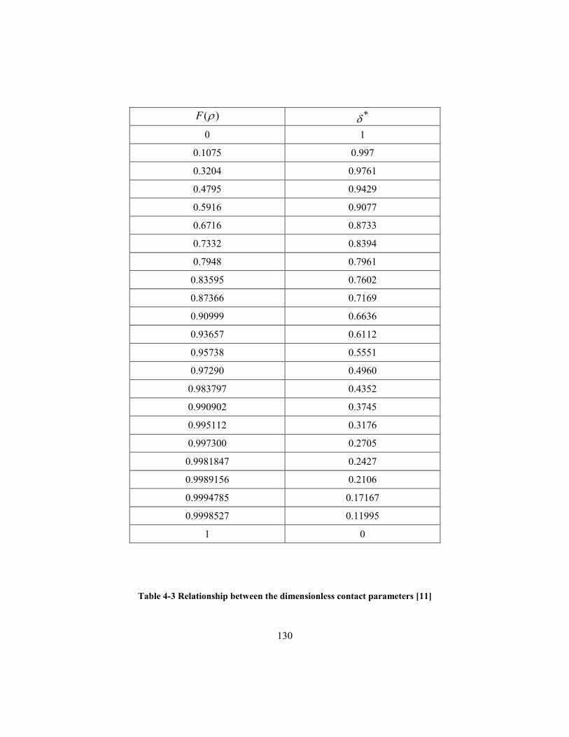
130
)(F *
0 1
0.1075 0.997
0.3204 0.9761
0.4795 0.9429
0.5916 0.9077
0.6716 0.8733
0.7332 0.8394
0.7948 0.7961
0.83595 0.7602
0.87366 0.7169
0.90999 0.6636
0.93657 0.6112
0.95738 0.5551
0.97290 0.4960
0.983797 0.4352
0.990902 0.3745
0.995112 0.3176
0.997300 0.2705
0.9981847 0.2427
0.9989156 0.2106
0.9994785 0.17167
0.9998527 0.11995
1 0
Table 4-3 Relationship between the dimensionless contact parameters [11]

131
The tangential contact-interaction force between the rolling-elements and the races is
assumed to be defined by the Coulomb law as:
nt FF (4–5)
where is the friction coefficient. Under the elastohydrodynamic conditions (associated with
the presence of a lubricant within the bearing element), is generally considered to be a
function of the rolling-element/race slip velocity, sV . The vs sV functional relationship used
in the present work was taken from [10] and is depicted in Figure 4-3. This functional
relationship was used in its tabulated form in the present work. The slip velocity between a
rolling-element and the inner-race, insV is defined in terms of the rolling-element revolving
velocity, revrV , the rolling-element rotational velocity, rotr and the inner-race rotational
velocity, racein as:
rollerrotrrevrraceinraceinins RVRV (4–6)
revrV is obtained using the following two-step procedure: (a) first, a component of the rolling-
element velocity vector (located within the x-z plane) in the (instantaneous) tangent direction is
determined; (b) then, this velocity component is multiplied by a ratio of the raceinR and rolling-
element/inner-race center-to-center distance. An analogous procedure is used to determine the
slip velocity at the rolling-element/outer-race contact interface, outsV and to establish its effect
on the associated friction coefficient (and, in turn, the tangential force).
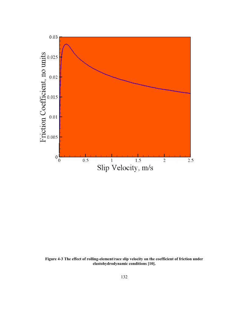
132
Figure 4-3 The effect of rolling-element/race slip velocity on the coefficient of friction under
elastohydrodynamic conditions [10].

133
The contact interactions between the rolling elements and the races are implemented as
user-defined force elements within the uforce20 SIMPACK subroutine. The kinematic
relationships between a rolling element and a contacting race is established through the use of a
“from” marker (a coordinate system attached to the center of the rolling element) and the “to”
marker (a coordinate system attached to the center of the race). Per request made by the user,
SIMPACK will provide the requested kinematic parameters within the two markers. For example,
the user may request the position vector of the from-marker origin relative to the to-marker origin
expressed in the global reference frame. This information can be used to compute and, in turn,
nF . SIMPACK expects the user to return to it the values of the interaction-force and interaction-
torque components all expressed in the reference-frame of the body associated with the from-
marker (a rolling-element, in the present case). Due to the regular-cylindrical geometry of the
rolling elements, their reference-frame is coincident with their from-marker. Thus, the interaction
forces and torques have to be returned in the from-marker coordinate system. It should be noted
that nF and tF act respectively in a direction normal to and in a direction tangential to the
rolling-element/race contact patch. To compute and superpose the components of nF and tF
along the axes of the from-marker, the following three-step procedure is used: (a) first, the
knowledge of the position vector of the from-marker origin relative to the to-marker origin
expressed in the global frame is first used to determine the directional cosines of the vectors
associated with nF and tF ; (b) this knowledge is used to project nF and tF to the global-frame
axes and to determine the resulting interaction-force components acting along the axes of the
global frame, and (c) lastly, SIMPACK is asked to provide a rotation matrix relating the from-
marker to the global frame and this rotational matrix is used to compute the interaction-force
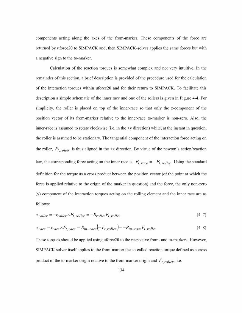
134
components acting along the axes of the from-marker. These components of the force are
returned by uforce20 to SIMPACK and, then SIMPACK-solver applies the same forces but with
a negative sign to the to-marker.
Calculation of the reaction torques is somewhat complex and not very intuitive. In the
remainder of this section, a brief description is provided of the procedure used for the calculation
of the interaction torques within uforce20 and for their return to SIMPACK. To facilitate this
description a simple schematic of the inner race and one of the rollers is given in Figure 4-4. For
simplicity, the roller is placed on top of the inner-race so that only the z-component of the
position vector of its from-marker relative to the inner-race to-marker is non-zero. Also, the
inner-race is assumed to rotate clockwise (i.e. in the +y direction) while, at the instant in question,
the roller is assumed to be stationary. The tangential component of the interaction force acting on
the roller, rollertF , is thus aligned in the +x direction. By virtue of the newton’s action/reaction
law, the corresponding force acting on the inner race is, rollertracet FF ,, . Using the standard
definition for the torque as a cross product between the position vector (of the point at which the
force is applied relative to the origin of the marker in question) and the force, the only non-zero
(y) component of the interaction torques acting on the rolling element and the inner race are as
follows:
rollertrollerrollertrollerroller FRFr ,, (4–7)
rollertraceinrollertraceinracetracerace FRFRFr ,,, (4–8)
These torques should be applied using uforce20 to the respective from- and to-markers. However,
SIMPACK solver itself applies to the from-marker the so-called reaction torque defined as a cross
product of the to-marker origin relative to the from-marker origin and rollertF , , i.e.

135
rollertraceinrollerreaction FRR , (4–9)
Since reaction is not equal to roller and no reaction torque is prescribed to the to-marker, one
must return to SIMPACK, not the actual torques acting on the from- and to-markers, but rather
corrections to reaction which should yield correct values for roller and race . This must be
done while recognizing that single torque (vector) returned by uforce20 to SIMPACK is applied
to the from-marker and a negative value of this torque to the to-marker. Simple examination of
Eqs. (4–5) to (4–7) reveals that the torque correction term (i.e. the torque which uforce20 will
return to SIMPACK) should be:
rollertraceincorrection FR , (4–10)
The net torque acting on the from-marker is then:
rollerrollertrollercorrectionreactionnetroller FR ,, (4–11)
Likewise, since correction is applied to the to-marker, the net torque acting on this marker is:
racerollertraceincorrectionnetrace FR ,, (4–12)

136
Figure 4-4 A schematic of the single-roller/inner-race contact pair used to explain the way the
contact-interaction torque is calculated within uforce20 and returned to SIMPACK.
X
Z
Y
rrace
rroller Ft, roller Ft, race = – Ft, roller
Inner Race
Roller

137
Rolling-elements/bearing-cage contact interactions
Force elements are also used to model interactions between each rolling element and the
respective pocket of the cage. One such force element was used per rolling element. In other
words, a single force element is used to model the interaction of a rolling element with both
leading and trailing bridges of respective cage pocket. To formulate a rolling-element/cage force
element, the from-marker is placed at the center of the rolling element. The respective pocket was
positioned symmetrically with respect to the rolling and the to-marker placed at the center of the
pocket. In this way, the two markers are made initially made coincident. The orientation of the
two markers is set to coincide with the radial, tangential and bearing-axial directions where, the
radial and tangential directions are defined by the initial position of the rolling element and the
bearing-element axis. To determine the interaction force, angular positions of the rolling-element
and the cage-pocket center are monitored. When the magnitude of the difference in these two
angular positions, )(abs , is larger than the one corresponding to the initial clearance between
the rolling-element and the cage-pocket bridge, )( criticalabs , the interaction force (in the
global frame) is assumed to acquire non-zero values as:
rollercage
rollercage
rollercage
rollercage
rollerraceincriticalcageroller
z
y
x
rr
zz
rr
xx
RRabsabsK
F
F
F
0)()( (4–13)
where cagerollerK denotes spring constant, r is the position vector of the respective marker, x
and z the corresponding components of this vector.

138
Potential problem with the implementation of Eq. (4–13) in uforce20 is that angular
positions of roller and/or cage can abruptly change by +/- 2 upon completion of a full
revolution. To identify such instances and prevent erroneous determination of the roller/cage
interaction force, )(abs was monitored closely for its abrupt change and an excessive value.
Details of this procedure can be inferred by analyzing uforce20 source code provided in the
APPENDIX A.

139
4.3.4 Construction of the User-defined Force Element
The In accordance with the SIMPACK user-subroutine format, uforce20 is composed of
three individual subroutines: (a) uforce20_type; (b) uforce20_setup; (c) uforce20. Within the
uforce20_type subroutine, the following tasks are accomplished: (i) user force-element name is
defined which is recognized by the SIMPACK GUI; (ii) global variables are defined by including
“simpack.ins” file; (iii) the nature of the element, force vs control is defined; and (iv) the number
of model parameters, dynamic states, output variables are specified. Within the uforce20_setup
subroutine, the following tasks are accomplished: (i) element specific parameters are defined; (ii)
parameters are checked by carrying out a pre-processing procedure; and (iii) names of the
parameters, dynamic states and output variables are specified. Within the uforce20 subroutine, the
main task is to, compute the forces and torques in the reference frame of the body associated with
the from-marker and return it to SIMPACK.
A script of the source codes of the three subroutines mentioned above for the cases of
force elements developed and used in the present work is provided in the APPENDIX A.

140
4.3.5 Kinematics-based Derivation of the Zero-Slip Roller Angular Velocity
In this section, an analytical procedure is used to derive equations relating the revolving
and rotational speeds of the rolling elements in contact with the inner and the outer races under
zero-slip conditions and the geometrical and kinematic parameters of the rolling elements and the
races. This procedure starts by defining the slip velocities at the rolling-element/inner-race and
rolling-element/outer-race surfaces and setting them both to zero as:
rollerrotrrollerracein
raceinrevrraceinracein
rollerrotrracein
revrraceinraceinins
RRR
RVR
RVRV
(4–13)
rollerrotrrollerraceout
raceoutrevrraceoutraceout
rollerrotrraceout
revrraceoutraceoutouts
RRR
RVR
RVRV
(4–14)
Eqs. (4–11) and (4–12) represent a linear system of two algebraic equations with two unknowns
which can be readily solved (analytically), to yield solutions for the unknown variables:
raceoutraceoutraceinraceinraceoutracein
rollerraceoutrevr RR
RR
RRV
(4–15)
raceinraceout
raceoutraceinroller
raceinraceoutrotr
RRR
RR
(4–16)
To validate the uforce20 code, MBD simulations are carried out within SIMPACK using a
number of combinations of racein and raceout . After a transient period each simulation
would begin to approach the steady (zero-slip) condition associated with nearly constant values of
revrV and rotr . The computed values of these quantities are then compared with their
analytical counterparts as defined respectively by Eqs. (4–13) and (4–14) to, judge the validity of

141
the contact-interaction force-element constitutive relations in uforce20. The results of this
comparison are presented in the next section.

142
4.4. Results and Discussion
As explained earlier, the work presented in this chapter was aimed at constructing the
foundation for a more comprehensive MBD computational investigation of the dynamic behavior
of a prototypical wind-turbine gear-box bearing element. The kinematic and kinetic behavior of
the roller bearings particularly during particular events/scenarios such as extreme gust, wind-
turbine emergency shutdown, wind-turbine restart, etc. is believed to be one of the main
contributors to the root cause of roller-bearing premature failure. The main objective of the work
presented in this chapter is to successfully implement user-defined contact-interaction force
elements into a SIMPACK user subroutine uforce20. The success of this implementation is
shown in Figure 4-5 and Figure 4-6. Figures 4–5 and 4–6 show respectively the variations of
revrV and rotr with racein and raceout , as contour plots. In the case of each figure,
part (a) shows the results as predicted by the analytical procedure presented in 4.3.5 while, part
(b) shows the corresponding results obtained directly through the use of uforce20 and SIMPACK.
A comparison of the results displayed in parts (a) and (b) of Figures 4–5 and 4–6 reveals that the
present implementation of the contact-interaction force elements in uforce20 and linking of this
subroutine with SIMPACK is correct.

143
Figure 4-5 The effect of the inner-race rotational speed and the outer-race rotational speed on the no-
slip revolving velocity of the rollers in the case of the roller-bearing being analyzed: (a) an analytical
kinematics-based solution; and (b) the numerical uforce20/SIMPACK based solution.

144
Figure 4-6 The effect of the inner-race rotational speed and the outer-race rotational speed on the no-
slip angular (rotational) velocity of the rollers in the case of the roller-bearing being analyzed: (a) an
analytical kinematics-based solution; and (b) the numerical uforce20/SIMPACK based solution.

145
The effect of the inner-race rotational velocity, for the case of the initially stationary
rolling elements and a zero rotational-velocity of the outer race, on the slip velocity at the
interfaces between the rolling elements and: (a) the inner; (b) the outer race is depicted in Figures
4–7(a)–(b), respectively. Examination of the results displayed in Figure 4-7(a) shows that: (a) as
expected, the initial slip velocity at the rolling-element/inner-race interface is simply a product of
the inner-race rotational velocity and the inner-race radius; and (b) the time required for the
roller-bearing to attain the no-slip state increases with an increase in the initial slip-velocity at the
rolling-element/inner-race interface. Furthermore, examination of the results displayed in Figure
4-7(b) shows that: (a) as expected, the initial slip velocity at the rolling-element/outer-race
interface is zero; and (b) as the simulation proceeds, the slip velocity at the rolling-element/outer-
race interface first begins to deviate from zero, attains the largest magnitude, and then gradually
begins to approach its zero value (corresponding to the no-slip condition at the rolling-
element/outer-race interface).

146
Figure 4-7 The effect of (constant) inner-race rotational velocity, for the case of the initially
stationary rolling elements and always stationary outer race, at the interfaces between the rolling
elements and: (a) the inner race; (b) the outer race.

147
4.5. Summary and Conclusions
Based on the results obtained in this portion of the work, the following main summary
remarks and conclusions can be drawn:
1. To facilitate future work related to the effect of unfavorable bearing kinematics on the
premature failure of wind-turbine gearboxes, a multi-body dynamics (MBD) computational
model has been developed for a prototypical roller bearing.
2. While constructing the MBD model for the bearing, standard built-in options available
in SIMPACK – a general purpose MBD code, such as rigid bodies, joints and kinematic
constraints are utilized.
3. To account more realistically for the interactions between rolling elements and the
inner/outer race as well as between rolling elements and cage/retainer, a set of user defined force
elements is constructed. To link these elements with SIMPACK solver, a user subroutine
uforce20 has been developed and validated.
4. The validity of the overall bearing-element MDB model is validated by comparing its
predictions and the corresponding close-form analytical results pertaining to the no-slip rotational
and revolving velocities of the rolling elements. In addition, the model is used to show the effect
of the magnitude of the transient-stage perturbation on the time required for the bearing to regain
its steady no-slip condition.
148
4.6. References
1. M. Grujicic, B. Pandurangan, Y. Huang, B. A. Cheeseman, W. N. Roy, and R. R. Skaggs,
“Impulse Loading Resulting from Shallow Buried Explosives in Water-saturated Sand”,
Journal of Materials: Design and Applications 221: 21-35, (2007a).
2. M. Grujicic, B. Pandurangan, U. Zecevic, K.L. Koudela, and B. A. Cheeseman, “Ballistic
Performance of Alumina/S-2 Glass-Reinforced Polymer-Matrix Composite Hybrid
Lightweight Armor Against Armor Piercing (AP) and Non-AP Projectiles,” Multidiscipline
Modeling in Materials and Structures 3: 287–312, (2007b).
3. M. Grujicic, and W.C. Bell, “A Computational Analysis of Survivability of a Pick-Up Truck
Subjected to Mine Detonation Loads,” Multidiscipline Modeling in Materials and Structures,
7: 386-423, (2011a).
4. W. D. Musial, S. Butterfield, and B. McNiff, “Improving Wind Turbine Gearbox
Reliability,” Proceedings of the European Wind Energy Conference, Milan, Italy, May 7–10,
2007.
5. ISO/IEC 81400-4:2005, “Wind Turbines – Part 4: Standard for Design and Specification of
Gear-boxes,” International Organization for Standardization, Geneva, Switzerland, 2005.
6. ISO 15243:2004, “Rolling bearings – Damage and failures – Terms, characteristics and
causes,” International Organization for Standardization, Geneva, Switzerland, 2004.
7. SKF Company Brochure. “Bearing Failures and Their Causes,” Publication Number 401 E.
Accessed August 8, 2013. http://www.skf.com/group/knowledge-centre/aptitude-
exchange/articles/index.html
8. K. Stadler and A. Stubenrauch, “Premature Bearing Failures in Industrial Gear-boxes,”
National Renewable Energy Laboratory. Accessed on August 8, 2013.
www.nrel.gov/wind/grc/pdfs/12_premature_bearing failures.pdf
9. SIMPACK Release 9.3, “SIMPACK Reference Guide,” SIMDOC v9.31, January 2013.
10. W. Tu, Y. Shao, and C. K. Mechefske, “An analytical model to investigate skidding in
rolling element bearings during acceleration,” Journal of Mechanical Science and
Technology, 26 (8), 2451-2458, 2012.
11. T. A. Harris, and M. N. Kotzalas, “Essential Concepts of Bearing Technology, Fifth
Edition,” CRC Press, 2006, ISBN: 978-1-4200-0659-9.

149
CHAPTER 5: CONCLUSIONS AND SUGGESTIONS FOR FUTURE WORK
5.1. Conclusions
While each of the chapters 2 through 4 contains a summary of the conclusions resulting
from the work reported in these chapters, a list of more general conclusions arrived at the end of
the present work is presented in the remainder of this section. This list includes:
1. Computer aided engineering (CAE) analysis and material selection methods and tools
have achieved the level of physical fidelity, computational robustness and accuracy that
they can greatly help in the design of a new horizontal axis wind turbine blades. Specific
areas in which these methods and tools could be particularly beneficial include
predictions of the blade’s structural integrity, its durability and reliability. The methods
and tools identified in the present work as having key role include finite element analysis,
Rainflow analysis, Goodman diagram, Miner’s rule, material selection charts and indices,
etc.
2. Computer aided engineering methods and tools can also play a major role in helping
identify the root cause method of the wind-turbine gearbox premature failure. In the
present work, this point was demonstrated by analyzing a particular mode of gearbox
failure (i.e. gear-tooth bending fatigue). To model this failure mode, advanced finite-
element structural/stress analysis is combined with the computational procedures
developed for prediction of fatigue-crack initiation and growth processes (and ultimate
failure). The results obtained clearly revealed the effect of the service-loading conditions
(as quantified by the transferred-torque and the gear-misalignment) on the fatigue-
service-life of the gearbox.
3. Since unfavorable kinematics of wind-turbine gear-box bearing elements is believed to be
one of the root causes of their premature failure. The starting point in approaching this

150
complex problem is establishment of reliable multi-body dynamics (MBD) model for a
prototypical cylindrical roller bearing. One of the most challenging aspects of such roller-
bearing MBD model is the establishment and evaluation of the forces and torques
generated as a result of contact interactions between rolling elements and inner-outer
races, as well as between the rolling elements and the cage/retainer. Such interactions are
quantified and validated in the present work through the use of a user-defined MBD force
element.

151
5.2. Suggestions for Future Work
The work reported in this thesis can be extended in a multiple directions. In the remainder
of this sub-section, one of such directions per topic covered in this thesis is briefly discussed.
1. The work presented in Chapter 2, can be naturally extended in the direction of a coupling
the computational analyses developed with a multi-objective/multi-constraint engineering
optimization analysis. Within such an optimization analysis, various aspects of the wind-
turbine performance such as its structural integrity, durability, reliability, weight, cost,
etc. can be simultaneously optimized by varying different blade-design and material
parameters while ensuring that the design and functional constraints are satisfied.
2. In the case of the work presented in Chapter 3, one extension would involve modeling of
the structural behavior (including failure) of wind turbine gears under the conditions of
bearing-debris being caught between the meshing teeth of the wind-turbine gears. These
conditions are occasionally found to lead to gear misalignment, excessive tooth-loading
and ultimate (premature) failure.
3. The work presented in Chapter 4 should be extended in the direction of modeling the
effect of unfavorable bearing kinematics (associated with various wind turbine transient
events, e.g. occasional gusts, emergency shutdown, startup, etc.) on the initiation of
surface and sub-surface damage within the bearing races, the phenomenon which is
believed to be closely related to the problem of wind-turbine gear-box roller-bearing
premature failure.

152
APPENDIX A: USER-DEFINED FORCE ELEMENT – UFORCE20 SOURCE CODE
User Defined Force Element is developed which calculates Contact Forces developed
within a Roller bearing, due to the interactions between the bearing elements. This subroutine
contains commented lines to help understand the logic in the code. This is used for the model
with 12 rolling elements to verfiy the analytical solution. Although the cage is present, it does not
affect steady state values but a force element applies forces or torques on it.
!*****************************************************************************
!> SIMPACK User Force/Control Element Type 20
!> Author: Varun (Dr.Grujicic Research Team)
!*****************************************************************************
subroutine uforce20_type( str_dim !< [in ] name string length
+ , type_name !< [out] force type name
+ , ierr !< [out] error code
+ )
#if defined(WINDOWS)
!DEC$ ATTRIBUTES DLLEXPORT::uforce20_type
#endif
C ----------------------------------------------------------------------
C Declaration of Global Variables
C ----------------------------------------------------------------------
implicit none
include 'simpack.ins'
C ----------------------------------------------------------------------
C Declaration of Interface Parameters
C ----------------------------------------------------------------------
integer :: str_dim
integer :: ierr
character(len=*) :: type_name
C ----------------------------------------------------------------------
C Initialization
C ----------------------------------------------------------------------
ierr = 0

153
C ----------------------------------------------------------------------
C Execution
C ----------------------------------------------------------------------
! name 123456789012345678901234567890'
! name of user-defined force element '
type_name = 'CRB Contact Forces '
call spck_df_FClass(fclass_force,ierr) ! force element
call spck_df_ForceParDim(10,ierr) ! parameters
call spck_df_ForceStDynDim(0,ierr) ! dynamic states
call spck_df_ForceOvDim(20,ierr) ! output values
return
end subroutine
!******************** END OF SUBROUTINE uforce20_type ************************
subroutine uforce20_setup( task !< [in ] |-1 | 5 | 0 | 1 | 2 | 4 | task flag
+ , par_dim !< [in ] | i | i | i | i | i | i | number of parameters
+ , stdyn_dim !< [in ] | i | i | i | i | i | i | number of dynamic states
+ , ov_dim !< [in ] | i | i | i | i | i | i | number of output values
+ , str_dim !< [in ] | i | i | i | - | - | - | max. length of names
+ , id !< [in ] | i | i | i | i | i | i | element id
+ , mk_from !< [in ] | i | i | i | i | i | i | from-marker id
+ , mk_to !< [in ] | i | i | i | i | i | i | to-marker id
+ , par !< [in,out] | i |i/o| i |i/o|i/o| i | parameters
+ , par_typ !< [ out] | - | - | o | - | - | - | parameter types
+ , par_str !< [ out] | - | - | o | - | - | - | parameter names
+ , par_u !< [ out] | - | - | o | - | - | - | parameter unit types
+ , stdyn_str !< [ out] | - | - | o | - | - | - | dynamic state names
+ , stdyn_u !< [ out] | - | - | o | - | - | - | dynamic state unit types
+ , ov_str !< [ out] | - | - | o | - | - | - | output value names
+ , ov_u !< [ out] | - | - | o | - | - | - | output value unit types
+ , res_flg !< [ out] | - | - | - | o | - | - | output flag
+ , stdyn_nr !< [ ] | - | - | - | - | - | - | (obsolete)
+ , stroot_nr !< [ ] | - | - | - | - | - | - | (obsolete)
+ , str_flg !< [ out] | - | - | - | o | - | - | state reset flag
+ , ierr !< [ out] | o | o | o | o | o | o | error code
+ )
#if defined(WINDOWS)
!DEC$ ATTRIBUTES DLLEXPORT::uforce20_setup
#endif
C ----------------------------------------------------------------------
C Declaration of Global Variables

154
C ----------------------------------------------------------------------
implicit none
include 'simpack.ins'
C ----------------------------------------------------------------------
C Declaration of Interface Parameters
C ----------------------------------------------------------------------
integer task
integer par_dim
integer stdyn_dim
integer ov_dim
integer str_dim
integer id
integer mk_from
integer mk_to
integer par_typ(par_dim)
integer par_u(par_dim)
integer stdyn_u(stdyn_dim)
integer ov_u(ov_dim)
integer res_flg
integer stdyn_nr
integer stroot_nr
integer str_flg
integer ierr
double precision :: par(par_dim)
character(len=*) :: par_str(par_dim)
character(len=*) :: stdyn_str(stdyn_dim)
character(len=*) :: ov_str(ov_dim)
C ----------------------------------------------------------------------
C Initialization
C ----------------------------------------------------------------------
ierr = 0
C ----------------------------------------------------------------------
C task = -1 : Parameter-dependent Dimensions
C ----------------------------------------------------------------------
if ( task .eq. -1 ) then
continue
C ----------------------------------------------------------------------
C task = 0 : Names and Types
C ----------------------------------------------------------------------
else if ( task .eq. 0 ) then
! initialise outputs

155
!-------------------
par_str(1:par_dim) = ' '
par_typ(1:par_dim) = knodef
par_u(1:par_dim) = knodef
stdyn_str(1:stdyn_dim) = ' '
stdyn_u(1:stdyn_dim) = knodef
ov_str(1:ov_dim) = ' '
ov_u(1:ov_dim) = knodef
! parameters
! ----------
! name '123456789012345678901234567890 ' | parameter type | unit type
! These parameter names will appear on the force element properties dialog box in
SIMPACK GUI
par_str( 1) = 'Nominal_Length ' ; par_typ( 1) = knr_double ; par_u( 1) = Kp_length
par_str( 2) = 'Normal_Stiffness ' ; par_typ( 2) = knr_double ; par_u( 2) = Kp_stiffness
par_str( 3) = 'Roller_Diameter ' ; par_typ( 3) = knr_double ; par_u( 3) = Kp_length
par_str( 4) = 'Race_Diameter ' ; par_typ( 4) = knr_double ; par_u( 4) = Kp_length
par_str( 5) = 'Race_Flag ' ; par_typ( 5) = knr_integer ; par_u( 5) = Kp_undefined
par_str( 6) = 'Critical_Angle ' ; par_typ( 6) = knr_double ; par_u( 6) = Kp_angle
! output values
! -------------
! name '123456789012345678901234567890' | unit type
! These output values names appear on FE properties in SIMPACK GUI
ov_str( 1) = 'Normal_Force ' ; ov_u( 1) = Kp_force
ov_str( 2) = 'Friction_Force ' ; ov_u( 2) = Kp_force
ov_str( 3) = 'Thrust_Force ' ; ov_u( 3) = Kp_force
ov_str( 4) = 'Friction_Torque ' ; ov_u( 4) = Kp_torque
ov_str( 5) = 'Normal_Fx ' ; ov_u( 5) = Kp_force
ov_str( 6) = 'Normal_Fz ' ; ov_u( 6) = Kp_force
ov_str( 7) = 'Tangential_Fx ' ; ov_u( 7) = Kp_force
ov_str( 8) = 'Tangential_Fz ' ; ov_u( 8) = Kp_force
ov_str( 9) = 'Total_Fx ' ; ov_u( 9) = Kp_force
ov_str(10) = 'Total_Fz ' ; ov_u(10) = Kp_force
ov_str(11) = 'V_slip ' ; ov_u(11) = Kp_velocity
ov_str(12) = 'Roller_Angle ' ; ov_u(12) = Kp_angle
ov_str(13) = 'V_Rev_Roller ' ; ov_u(13) = Kp_velocity
ov_str(14) = 'Cage_Angle ' ; ov_u(14) = Kp_angle
ov_str(15) = 'cage_pos_x ' ; ov_u(15) = Kp_length
ov_str(16) = 'roller_pos_x ' ; ov_u(16) = Kp_length
C ----------------------------------------------------------------------
C task = 1 : Element-specific Infos
C ----------------------------------------------------------------------
else if ( task .eq. 1 ) then

156
res_flg = 3 ! output flag
str_flg = 0 ! state reset flag (see also spck_slv_StRstInit)
stdyn_nr = 0 ! Number of Force States
stroot_nr = 0 ! Number of Root Functions
C ----------------------------------------------------------------------
C task = 2 : Check Parameters and Pre-Processing
C ----------------------------------------------------------------------
else if ( task .eq. 2 ) then
continue
C ----------------------------------------------------------------------
C task = 4 : Final Call
C ----------------------------------------------------------------------
else if ( task .eq. 4 ) then
continue
C ----------------------------------------------------------------------
C task = 5 : Default Parameters
C ----------------------------------------------------------------------
else if ( task .eq. 5 ) then
continue
end if
return
end subroutine
!*********************** END OF SUBROUTINE uforce20_setup ********************
subroutine uforce20( task !< [in ] | 0 | 1 | 2 | 3 | 4 | task flag
+ , par_dim !< [in ] | i | i | i | i | i | number of parameters
+ , uin_dim !< [in ] | i | i | i | i | i | number of u-vector components
+ , stdyn_dim !< [in ] | i | i | i | i | i | number of dynamic states
+ , stroot_dim !< [in ] | i | i | i | i | i | number of root states
+ , ov_dim !< [in ] | i | i | i | i | i | number of output values
+ , id !< [in ] | i | i | i | i | i | element id
+ , par !< [in ] | i | i | i | i | i | parameters
+ , mk_from !< [in ] | i | i | i | i | i | from-marker id
+ , mk_to !< [in ] | i | i | i | i | i | to-marker id
+ , time !< [in ] | i | i | i | i | i | time
+ , uin !< [in ] | i | i | i | i | i | u-vector
+ , stdyn !< [in,out] | i | i | i | i |i/o| dynamic states
+ , stroot !< [in,out] |i/o| i | i | i |i/o| root states
+ , stdynd !< [ out] | o | - | - | - | - | dynamic state derivatives
+ , force !< [ out] | o | - | - | - | - | force vector acting at from-marker w.r.t. from-brf
+ , torque !< [ out] | o | - | - | - | - | torque vector acting at from-marker w.r.t. from-brf
157
+ , ov !< [ out] | o | - | - | - | - | output values
+ , valroot !< [ out] | - | o | - | - | - | root function values
+ , ierr !< [ out] | o | o | o | o | o | error code
+ )
#if defined(WINDOWS)
!DEC$ ATTRIBUTES DLLEXPORT::uforce20
#endif
C ----------------------------------------------------------------------
C Declaration of Global Variables
C ----------------------------------------------------------------------
implicit none
include 'simpack.ins'
C ----------------------------------------------------------------------
C Declaration of Interface Parameters
C ----------------------------------------------------------------------
integer task
integer par_dim
integer uin_dim
integer stdyn_dim
integer stroot_dim
integer ov_dim
integer id
integer mk_from
integer mk_to
integer stroot(stroot_dim)
integer ierr
integer err
double precision par(par_dim)
double precision time
double precision uin(uin_dim)
double precision stdyn(stdyn_dim)
double precision stdynd(stdyn_dim)
double precision force(3)
double precision torque(3)
double precision ov(ov_dim)
double precision valroot(stroot_dim)
character(len=50) :: message
C ----------------------------------------------------------------------
C Declaration of Local Variables
C ----------------------------------------------------------------------
158
double precision zero
parameter(zero = 0.0d+00)
double precision PI
parameter(PI = 3.141592654)
! Input Parameters ---------------
double precision Nominal_Length ! The length of the force element (spring) at which
normal force is zero
double precision Normal_Stiffness ! The stiffness of roller-race/-cage contact, normal to
contact surface
double precision Roller_Diameter ! Diameter of the cylindrical rolling element
double precision Race_Diameter ! Outer Diameter of the Inner Raceway and Inner Diameter
of the Outer Raceway
integer Race_Flag ! Flag used to detect which contact interface is being analyzed
double precision Critical_Angle ! Critical value of angular displacement between cage and
roller
! Variables to calculate position of roller center
double precision d_roller ! distance between the roller center and the race center
double precision delta_r ! difference between distance and the nominal length of the userFE
double precision xyz_cmp_roller(3) ! cmps of position vector of roller center relative to race
center
double precision roller_pos_x ! x position of the roller center
double precision roller_pos_y ! y position of the roller center
double precision roller_pos_z ! z position of the roller center
! Variables to calculate position of cage pocket center
double precision d_cage ! distance between the roller center and the cage pocket center
double precision xyz_cmp_cage(3)! cmps of position vector of cage pocket center relative to
race center
double precision cage_pos_x ! x position of the cage pocket center
double precision cage_pos_y ! y position of the cage pocket center
double precision cage_pos_z ! z position of the cage pocket center
double precision delta_angle ! difference between angular position of cage pocket center and
roller center
double precision delta_cage ! circumferential displacement between roller center and cage
pocket center
! Variables to calculate distance between the roller center and the cage pocket center
double precision x_distance ! difference between x-components of the roller-to-cage
double precision z_distance ! difference between z-components of the roller-to-cage
double precision d_cage_roller ! distance between the roller center and cage pocket center
! Parameters to calculate velocities of rolling elements
double precision Omega_Roller ! rotational velocity of the roller about its own axis
double precision Velocity_Roller ! tangential (peripheral) velocity of the roller

159
double precision Omega_Race ! rotational velocity of the race
double precision Velocity_Race ! tangential (peripheral) velocity of the race
double precision Omega_Rev_Roller ! rotational velocity of the roller center (revolution)
about bearing axis
double precision Tang_Vel_Roller ! tangential velocity of roller center at the roller-race
contact interface
double precision V_abs ! magnitude of velocity of roller center relative to Global Ref. Frame
double precision V_ptp ! magnitude of velocity of roller center relative to Global Ref, Frame
double precision V_cmp(3) ! cmps of velocity vector of roller center relative to Global Ref.
Frame
! Parameters to evaluate the friction coefficient
double precision Min_Slip_Vel ! Value of Slip Velocity beyond which Mu is constant
double precision Min_Friction_Coeff ! Value of Friction Coefficient when Slip Velocity = 0
double precision Max_Friction_Coeff ! Value of Friction Coefficient when Slip Velocity =
Min Slip Vel
double precision Slope ! Slope of the linear part of the curve
double precision Mu ! Coefficient of Friction
double precision trmat_roller(3,3) ! Transformation Matrix between global frame and roller
center
! Output Parameters -----------------
double precision Normal_Force ! Magnitude of force normal to roller-race/-cage contact
interface
double precision Friction_Force ! Magnitude of Force tangential to contact interface
double precision Thrust_Force ! Magnitude of Force perpendicular to bearing plane
double precision Friction_Torque ! Magnitude of Torque applied to contacting bodies
double precision Normal_Fx ! Normal Force component in x-dir of Global Ref. Frame
double precision Normal_Fz ! Normal Force component in z-dir of Global Ref. Frame
double precision Tangential_Fx ! Tangential Force component in x-dir of Global Ref. Frame
double precision Tangential_Fz ! Tangential Force component in z-dir of Global Ref. Frame
double precision Total_Fx ! Total Force component in x-dir of Global Reference Frame
double precision Total_Fz ! Total Force component in z-dir of Global Reference Frame
double precision V_slip ! Relative velocity at the roller-race contact interface
double precision Roller_Angle ! Angle defining the angular position of the roller center
double precision V_Rev_Roller ! translational velocity of the roller center
double precision Cage_Angle ! Angle defining the angular position of the cage pocket
c ----------------------------------------------------------------------
c User defined parameters
c ----------------------------------------------------------------------
Nominal_Length = par( 1)
Normal_Stiffness = par( 2)
Roller_Diameter = par( 3)
Race_Diameter = par( 4)

160
Race_Flag = par( 5)
Critical_Angle = par( 6)
C ----------------------------------------------------------------------
C Initialization
C ----------------------------------------------------------------------
ierr = 0
C ----------------------------------------------------------------------
C task = 0 : Determine force, torque and output values
C ----------------------------------------------------------------------
if ( task .eq. 0 ) then
c ! Calculate the Normal Force ****************
c ----------------------------------------------------------------
! Roller-Race Contact Interface *************
! ------------------------------------------------------------
! Calculate angular position of Roller Center relative to z-axis of Global ($M_Isys)
call SPCK_AV_DXYZ(d_roller,xyz_cmp_roller,mk_from,0,0,ierr)
delta_r = d_roller - Nominal_Length
roller_pos_x = xyz_cmp_roller(1)
roller_pos_y = xyz_cmp_roller(2)
roller_pos_z = xyz_cmp_roller(3)
if (roller_pos_x.lt.zero) then
Roller_Angle = 2*PI + atan2(roller_pos_x,roller_pos_z)
else
Roller_Angle = atan2(roller_pos_x,roller_pos_z)
end if
! Calculate the magnitude of the Normal Force at roller-race contact interface
if (Race_Flag.eq.1) then
if (d_roller.lt.Nominal_Length) then
Normal_Force = Normal_Stiffness*(-delta_r)**(3.0/2.0)
else
Normal_Force = zero
end if
else if (Race_Flag.eq.2) then
if (d_roller.gt.Nominal_Length) then
Normal_Force = -Normal_Stiffness*(delta_r)**(3.0/2.0)
else
Normal_Force = zero
end if
end if
! Calculate components of Normal Force in $M_Isys for roller-race contact interface

161
if (Race_Flag.eq.1.or.Race_Flag.eq.2) then
Normal_Fx = Normal_Force * sin(Roller_Angle)
Normal_Fz = Normal_Force * cos(Roller_Angle)
end if
! Roller-Cage Contact Interface ***********************
! ----------------------------------------------------------------------------
! Calculate angular position of Cage-Pocket Center relative to z-axis of $M_Isys
if (Race_Flag.eq.3) then
call SPCK_AV_DXYZ(d_cage,xyz_cmp_cage,mk_to,0,0,ierr)
cage_pos_x = xyz_cmp_cage(1)
cage_pos_y = xyz_cmp_cage(2)
cage_pos_z = xyz_cmp_cage(3)
if (cage_pos_x.lt.zero) then
Cage_Angle = 2*PI + atan2(cage_pos_x,cage_pos_z)
else
Cage_Angle = atan2(cage_pos_x,cage_pos_z)
end if
else
Cage_Angle = zero
end if
! Calculate distance between cage pocket center and roller center
! The vector is drawn from roller center to the cage pocket center
if (Race_Flag.eq.3) then
x_distance = (cage_pos_x - roller_pos_x)
z_distance = (cage_pos_z - roller_pos_z)
d_cage_roller = sqrt(x_distance**2.0 + z_distance**2.0)
else
cage_pos_x = zero
end if
! Calculate the magnitude of the Normal Force at roller-cage contact interface
if (Race_Flag.eq.3) then
delta_angle = Roller_Angle - Cage_Angle
if (delta_angle.lt.-PI) then
Cage_Angle = Cage_Angle - 2*PI
end if
if (delta_angle.gt.PI) then
Roller_Angle = Roller_Angle - 2*PI
end if
delta_angle = Roller_Angle - Cage_Angle
delta_cage = (abs(delta_angle) - Critical_Angle)*d_cage
if (abs(delta_angle).gt.Critical_Angle) then
Normal_Force = (Normal_Stiffness/100)*(delta_cage)
else

162
Normal_Force = zero
end if
end if
! Calculate components of Normal Force in $M_Isys for roller-cage contact interface
if (Race_Flag.eq.3) then
if (d_cage_roller.eq.zero) then
Normal_Fx = zero
Normal_Fz = zero
else
Normal_Fx = Normal_Force * (x_distance)/d_cage_roller
Normal_Fz = Normal_Force * (z_distance)/d_cage_roller
end if
end if
c ! Calculate the Tangential Force *******************************
c -------------------------------------------------------------------------------------------
! Calculate Tangential Velocity of the roller at the contact interface
! Rotation -----------------------------------------
call SPCK_AS_WY(Omega_Roller,mk_from,0,0,ierr)
Velocity_Roller = Omega_Roller * (Roller_Diameter/2)
! Calculate Tangential Velocity of the race at the contact interface
call SPCK_AS_WY(Omega_Race,mk_to,0,0,ierr)
Velocity_Race = Omega_Race * (Race_Diameter/2)
! Calculate Translational Velocity of the roller center
! Revolution ----------------------------------------------------
call SPCK_AV_VXYZ(V_abs,V_ptp,V_cmp,mk_from,0,0,0,ierr)
V_Rev_Roller = V_cmp(1) * cos(Roller_Angle)
& - V_cmp(3) * sin(Roller_Angle)
! Calculate Tangential Velocity of roller center at contact interface
Omega_Rev_Roller = V_Rev_Roller/d_roller
Tang_Vel_Roller = Omega_Rev_Roller * (Race_Diameter/2)
! Calculate Slip Velocity between the surfaces at the contact interface
if (Race_Flag.eq.1) then
V_slip = Velocity_Roller + Velocity_Race - Tang_Vel_Roller
else
V_slip = -Velocity_Roller + Velocity_Race - Tang_Vel_Roller
end if
! Calculate the Friction Coefficient which is a function of Slip Velocity
Min_Slip_Vel = 0.2
Min_Friction_Coeff = 0.0010

163
Max_Friction_Coeff = 0.03
Slope = Max_Friction_Coeff/Min_Slip_Vel
if (abs(V_slip).le.Min_Slip_Vel) then
Mu = Min_Friction_Coeff + Slope*abs(V_slip)
else
Mu = Max_Friction_Coeff
end if
! Determine the direction of Friction Force based on the Slip Velocity
if (Race_Flag.eq.1) then
if (V_slip.gt.0.0) then
Friction_Force = Mu*Normal_Force
else
Friction_Force = -Mu*Normal_Force
end if
elseif (Race_Flag.eq.2) then
if (V_slip.gt.0.0) then
Friction_Force = -Mu*Normal_Force
else
Friction_Force = Mu*Normal_Force
end if
else
Friction_Force = zero
end if
! Calculate the components of Tangential Force in Global Reference Frame ($M_Isys)
Tangential_Fx = Friction_Force * sin(Roller_Angle + (PI/2))
Tangential_Fz = Friction_Force * cos(Roller_Angle + (PI/2))
c ! Calculate the Axial Force ******************
c ----------------------------------------------------------------
! Calculate Thrust Forces (Axial Direction)
Thrust_Force = zero
c ! Calculate Total Force *********************
c ----------------------------------------------------------------
! Calculate the components of Total Force in Global Reference Frame ($M_Isys)
! Roller-Race Contact Interface and Roller-Cage Contact Interface
Total_Fx = Normal_Fx + Tangential_Fx
Total_Fz = Normal_Fz + Tangential_Fz
c ! Calculate the Torque **********************
c -----------------------------------------------------------------

164
! Calculate Moment (Torque about the roller y-axis)
Friction_Torque = Friction_Force*(Race_Diameter/2)
c ! Transform the Forces into Roller BRF ("From" Body BRF)
c --------------------------------------------------------------------------------
call SPCK_AV_TrMat(trmat_roller,mk_from,0,ierr )
! Assign force values using transpose of trmat_roller
! -----------------------------------------------------------------
force(1) = trmat_roller(1,1)*Total_Fx
& + trmat_roller(2,1)*Thrust_Force + trmat_roller(3,1)*Total_Fz
force(2) = trmat_roller(1,2)*Total_Fx
& + trmat_roller(2,2)*Thrust_Force + trmat_roller(3,2)*Total_Fz
force(3) = trmat_roller(1,3)*Total_Fx
& + trmat_roller(2,3)*Thrust_Force + trmat_roller(3,3)*Total_Fz
! Assign torque values
! ---------------------------------
torque(1) = zero
torque(2) = Friction_Torque
torque(3) = zero
if (Race_Flag.eq.3) then
torque(1) = zero
torque(2) = zero
torque(3) = zero
end if
! Update output values
! ----------------------------
ov(1) = Normal_Force
ov(2) = Friction_Force
ov(3) = Thrust_Force
ov(4) = Friction_Torque
ov(5) = Normal_Fx
ov(6) = Normal_Fz
ov(7) = Tangential_Fx
ov(8) = Tangential_Fz
ov(9) = Total_Fx
ov(10) = Total_Fz
ov(11) = V_slip
ov(12) = Roller_Angle
ov(13) = V_Rev_Roller

165
ov(14) = Cage_Angle
ov(15) = cage_pos_x
ov(16) = roller_pos_x
continue
C ----------------------------------------------------------------------
C task = 1 : Evaluate root functions
C ----------------------------------------------------------------------
else if ( task .eq. 1 ) then
continue
C ----------------------------------------------------------------------
C task = 2 : Perform state reset after root state switch
C ----------------------------------------------------------------------
else if ( task .eq. 2 ) then
continue
C ----------------------------------------------------------------------
C task = 3 : Determine algebraic state residuals
C ----------------------------------------------------------------------
else if ( task .eq. 3 ) then
continue
C ----------------------------------------------------------------------
C task = 4 : Initialise states after calculation of consistent states
C ----------------------------------------------------------------------
else if ( task .eq. 4 ) then
continue
end if
return
end subroutine
!************************ END OF SUBROUTINE uforce20 ************************