Parameterized Vertical-Axis Wind Turbine Wake

Model Using CFD Vorticity Data

Eric B. Tingey∗ and Andrew Ning†

Brigham Young University, Provo, Utah, 84602, USA

In order to analyze or optimize a wind farm layout, reduced-order wake models areoften used to estimate the interactions between turbines. While many such models exist forhorizontal-axis wind turbines, for vertical-axis wind turbines (VAWTs) a simple parametricwake model does not exist. Using computational fluid dynamic (CFD) simulations wecomputed vorticity in a VAWT wake, and parameterized the data based on normalizeddownstream positions, tip-speed ratio, and solidity to predict a normalized wake velocitydeficit. When compared to CFD, which takes about a day to run one simulation, thereduced-order model predicts the velocity deficit at any location within 5-6% accuracy ina matter of milliseconds. The model was also found to agree well with trends observed inexperimental data. Future additions will allow the reduced-order model to be used in windfarm layout analysis and optimization by accounting for multiple wake interactions.

Nomenclature

D turbine diameterF sigmoid curve decay rateI sigmoid curve inflection pointM sigmoid curve maximum valueN number of turbine bladesR turbine radiusU∞ free stream velocityα EMG skew parameterγ vorticity strengthκ EMG scale parameterλ tip-speed ratio= (ωR) /U∞ν EMG spread parameterω rotation rateσ solidity= (Nc) /Rξ EMG location parameterc chord lengthu velocity in the downstream directionx downstream positionxo specified downstream position for velocity calculationy lateral positionyo specified lateral position for velocity calculation

∗Graduate Student, Department of Mechanical Engineering, AIAA Student Member†Assistant Professor, Department of Mechanical Engineering, AIAA Senior Member

1 of 12

American Institute of Aeronautics and Astronautics

I. Introduction

Wind energy is receiving increased interest as an alternative source of power and currently researchersare pushing to move wind turbines to offshore locations where the wind is stronger and more consistent

than land-based locations.1 However, one of the difficulties in using turbines in offshore locations is thelarge cost required to install and maintain turbines in ocean environments.2 Horizontal-axis wind turbines(HAWTs), the type of wind turbine generally used in large-scale land-based applications, are difficult tomaintain because their drivetrain is located at the top of the tower and servicing it in offshore environmentsrequires the use of expensive sea vessels.3 HAWTs also require yaw and pitch systems to align the turbinewith the wind direction and regulate power, adding additional maintenance costs.4

Vertical-axis wind turbines (VAWTs) solve many of these challenges due to their simpler design andoperation. The VAWT drivetrain can be located near the base affording easier access5 and VAWTs can bemade smaller than HAWTs allowing more of them to be used in the same area as a HAWT wind farm,4

which could be beneficial for use in crowded urban environments. Additionally, VAWTs operate effectivelyno matter which way the wind is blowing, eliminating the need for a complex yaw system. These featuresmake VAWTs a potential concept for better offshore and urban power production.5,6

However, a current problem with using VAWTs in large wind farm optimization is the lack of a simplemodel to predict how wakes propagate behind VAWTs. In the wake of a turbine, wind has less momentumand more turbulence which propagates downstream, potentially decreasing the power production of otherturbines.7–9 When optimizing the cost of energy (total cost of the turbine divided by annual energy pro-duction) of many wind turbines in a wind farm, calculating the wake velocity deficit behind each turbine isdone to determine the optimal wind farm layout. Using higher-fidelity modeling for these calculations, whileproducing accurate wake velocity results, could take large amounts of time to obtain results. This processtakes even longer as the number of turbines increases with recalculations of the complex wake interactionsdone every time a turbine’s position changes. Reduced-order wake models address this problem by parame-terizing experimental wake behavior into simple mathematical models which can accurately predict the wakevelocity deficits much more quickly than higher-fidelity modeling. Optimization of wind farm layouts withreduced-order wake models for HAWTs has been studied extensively,10–16 but this same type of optimizationhas not been done with VAWTs because a reduced-order wake model does not exist.

Although a wake model does not exist, there have been several studies involving the operation of VAWTsand the wakes they produce. In the 1970s and 1980s, Sandia National Laboratories conducted researchcomparing the performance of different types of VAWT designs.17–19 The focus of the research was to under-stand VAWT power output and efficiency, and their efforts resulted in a compilation of blade aerodynamicproperties and power for different VAWT configurations. More recently, Delft University of Technologyin the Netherlands conducted research based on the near wake formation of VAWTs using particle imagevelocimetry (PIV) which provided significant insight into the near wake development of VAWTs and a knowl-edge of contributing factors in turbine wake behavior.20–24 Shamsoddin and Porte-Agel also conducted wakeresearch looking further downstream of a VAWT using large eddy simulation (LES) which showed goodagreement between the experiments and LES models.25 While all of these efforts have been significant inhelping us better understand the operation of VAWTs and how their wakes form, they have all been focusedmainly on a specific VAWT configuration. However, large-scale wind turbine analysis requires parametricwake models that can predict a velocity profile based on different turbine parameters such as wind speed,rotation rate, and geometry.

Research at the California Institute of Technology proposed a wake model using a single point vortex anda doublet to simulate a VAWT (rotating cylinder flow). It also used simple expansion and decay models topredict the wake velocity distribution.26 While this was a good first step in modeling a VAWT wake usinga simple model, it is not particularly accurate and is not able to be used in a generalized sense as it wastuned to a specific turbine. Therefore, the purpose of our research is to create a robust parametric VAWTwake model by studying the behavior of VAWT wakes over a large range of wind speeds, rotation rates, andgeometries. The model will be developed to allow for the optimization of a wind farm layout using VAWTsin a reasonable amount of time.

2 of 12

American Institute of Aeronautics and Astronautics

II. CFD Modeling

To produce a robust parametric wake model, flow around the turbine must be calculated based on varyingconditions, such as the size of the turbine and how fast it rotates. Performing a wake analysis of a specificturbine limits a model’s ability to calculate velocity accurately for a broad range of turbines. As our wakemodel was to be robust, we needed a large amount of wake data to predict how wakes propagate behindturbines at different wind speeds, rotation rates, and turbine geometries. We used computational fluiddynamics (CFD) software to simulate the turbines, as opposed to experimental procedures, as we needed awide range of configurations. Using a CFD program called STAR-CCM+, we simulated an isolated VAWTwith different tip-speed ratios (TSRs) and solidities using the unsteady 2D Reynolds-averaged Navier-Stokesequations, each which took about a day to compute. We modeled the VAWT in 2D rather than 3D as thefundamental process of energy conversion of a VAWT happens in the plane normal to the turbine’s axis ofrotation.21 While a 2D simulation does not account for finite blade effects, such as trailing and tip vortices,good agreement with experimental data was observed as noted in the validation studies.

Verification and validation of the CFD model is necessary to ensure that the model’s cell size is refinedenough and is producing results comparable to experimental data. For the verification, we performed a gridconvergence study of a model based on a study of a straight-bladed VAWT conducted by Kjellin et al.27 Wealso performed a validation study using a PIV wake analysis conducted by Tescione et al.20

A. CFD Mesh Verification

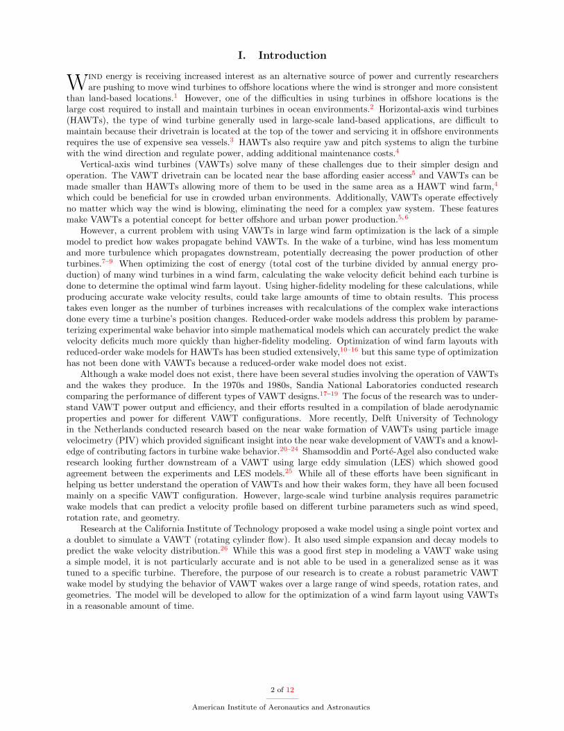
In order to verify that the cell size of the CFD model was sufficiently refined, we performed a grid convergencestudy. To accomplish this, we modeled a turbine using the geometry specified by Kjellin et al.27 including astraight-bladed VAWT with a 6 meter diameter and three NACA 0021 blades, each with a chord length of0.25 meters. The wind speed was set at 15 m/s producing a Reynolds number of about 6,000,000. Keepingthe TSR at 3.25 (at about the peak of performance from the experimental study), we ran simulations rangingfrom cell counts of about 400,000 to almost 5 million by reducing the base cell size of the CFD model by afactor of 1.4. The results of this grid convergence study can be seen in Fig. 1.

106 107

Cell Count

0.32

0.34

0.36

0.38

0.40

0.42

0.44

0.46

0.48

0.50

Pow

er C

oeff

icie

nt (C

P) Converged ValueEr

ror B

and

Figure 1. A plot of the grid convergence of the CFD model at a tip-speed ratio of 3.25. The converged valuecalculated with Richardson extrapolation is shown as well as the error band of the converged value. The modelwe used in our research is indicated by the red dot.

Using Richardson extrapolation, we concluded that the converged power coefficient was 0.458 with anerror band of 3.73%. In ideal circumstances, one would run the CFD models as refined as possible, butfurther refinement means more computational time for the CFD to reach a final solution. Therefore, abalance must be made between computational run time and sufficient refinement. In our case, we decidedthat about 630,000 cells was good enough for our CFD model as it produced a power coefficient of 0.432(within the error band) while still running in a reasonable amount of time (this point is indicted by the reddot in Fig. 1).

3 of 12

American Institute of Aeronautics and Astronautics

B. Wake Velocity Validation

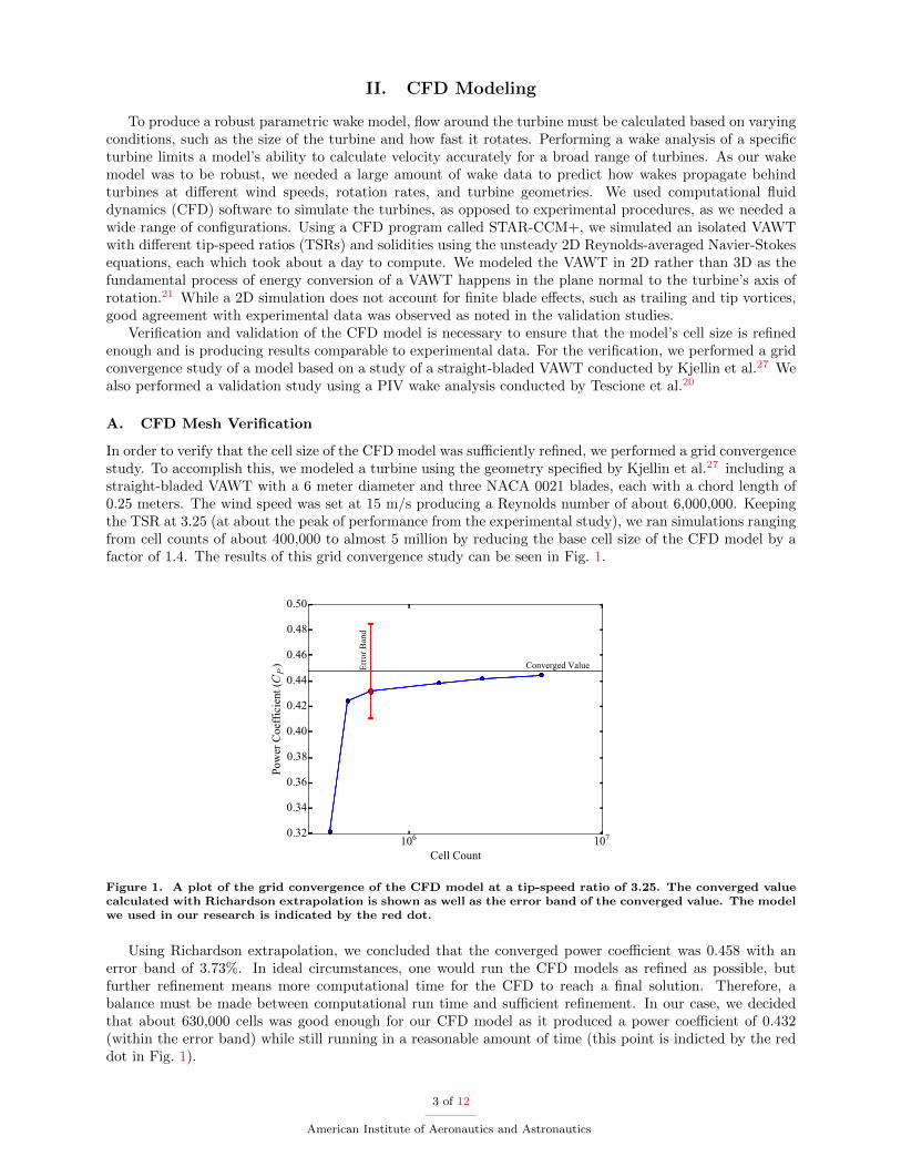
We also validated the wake velocity of the CFD model to ensure that the CFD cell size was refined enoughin the wake region. To do this, we used a study conducted by Tescione et al.20 in which a small turbine wastested in a wind tunnel at Delft University and velocities were measured with PIV. The turbine consisted oftwo straight NACA 0018 blades with a chord length of 0.06 meters. The turbine had a diameter of 1 meterand solidity of 0.24. The VAWT was tested in a wind speed of 9.3 m/s, producing a Reynolds number ofabout 180,000, and run at a TSR of 4.5.

The CFD model matched the PIV data well, as can be seen in Fig. 2, with the largest percent errorof 23.0% of the maximum velocity deficit at x/D = 2.0. This difference, as well as the asymmetry of theexperimental data, could be due to the differences in experimental setup as opposed to ideal wind conditionsin the CFD model. It is also reported that the asymmetry is caused by wake self-induction and strongervorticity on one side.20 We concluded that the CFD model was sufficiently refined to use in obtaining VAWTwake data for our reduced-order model. This wake validation study also served as a point of reference forvalidating the reduced-order model as will be described later in the paper.

1.0 0.5 0.0 0.5 1.0y/D

0.10.20.30.40.50.60.70.80.91.0

u/U

∞

x/D = 0.75

1.0 0.5 0.0 0.5 1.0y/D

0.10.20.30.40.50.60.70.80.91.0

u/U

∞

x/D = 1.0

1.0 0.5 0.0 0.5 1.0y/D

0.10.20.30.40.50.60.70.80.91.0

u/U

∞

x/D = 1.25 PIVCFD

1.0 0.5 0.0 0.5 1.0y/D

0.10.20.30.40.50.60.70.80.91.0

u/U

∞

x/D = 1.5

1.0 0.5 0.0 0.5 1.0y/D

0.10.20.30.40.50.60.70.80.91.0

u/U

∞

x/D = 1.75

1.0 0.5 0.0 0.5 1.0y/D

0.10.20.30.40.50.60.70.80.91.0u/U

∞x/D = 2.0

Figure 2. The wake velocity comparison between the PIV study conducted by Tescione et al.20 and our CFDmodel. The velocity (u) is normalized by the free stream wind velocity (U∞) and the downstream (x) andlateral (y) positions are normalized by the turbine diameter (D).

III. Reduced-Order Model Development

The purpose of a reduced-order wake model is to simulate wake propagation accurately and quickly. Inlarge-scale optimization, these benefits are used to produce results in a reasonable amount of time. As alreadyshown, we were able to use CFD modeling to calculate the velocity in a VAWT wake accurately in about aday. However, when many turbines are involved and moving them to a new position requires new calculations,large-scale applications of this method become very time-consuming. Therefore, the performance of reduced-order wake models are an improvement to a CFD analysis when analyzing large amounts of turbines.

For our research, we used the CFD models for different VAWT simulations at TSRs ranging from 2.5to 7.0 and solidities ranging from 0.15 to 1.0 based on the turbine diameter, airfoil shape, and Reynoldsnumber described by Kjellin et al.27 and each CFD simulation took about a day to compute the results.However, as can be seen in Fig. 3(a), trying to capture trends of the CFD velocity profiles with numericalmodels would be very complicated as it would require parametrically modeling the velocity profile in thefluid domain both inside and outside of the wake region. Therefore, we decided to use the vorticity data asseen in Fig. 3(b) with its concentrated streams which can be parametrically modeled easily. The vorticity

4 of 12

American Institute of Aeronautics and Astronautics

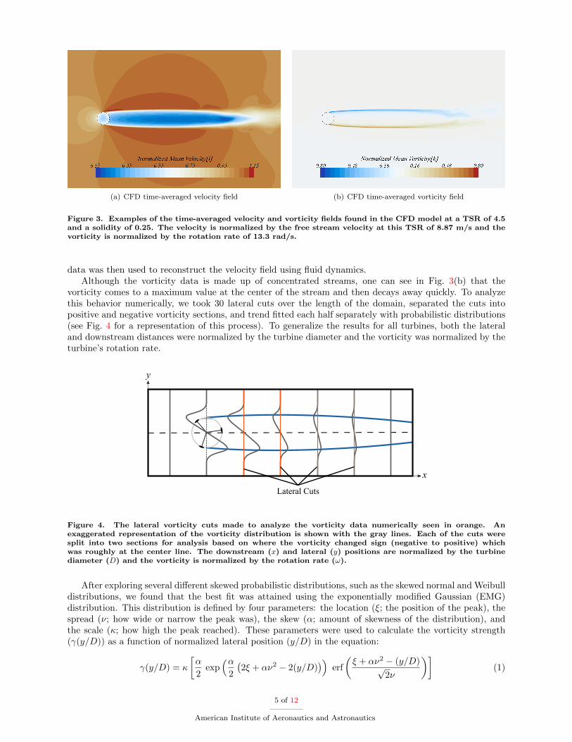
(a) CFD time-averaged velocity field (b) CFD time-averaged vorticity field

Figure 3. Examples of the time-averaged velocity and vorticity fields found in the CFD model at a TSR of 4.5and a solidity of 0.25. The velocity is normalized by the free stream velocity at this TSR of 8.87 m/s and thevorticity is normalized by the rotation rate of 13.3 rad/s.

data was then used to reconstruct the velocity field using fluid dynamics.Although the vorticity data is made up of concentrated streams, one can see in Fig. 3(b) that the

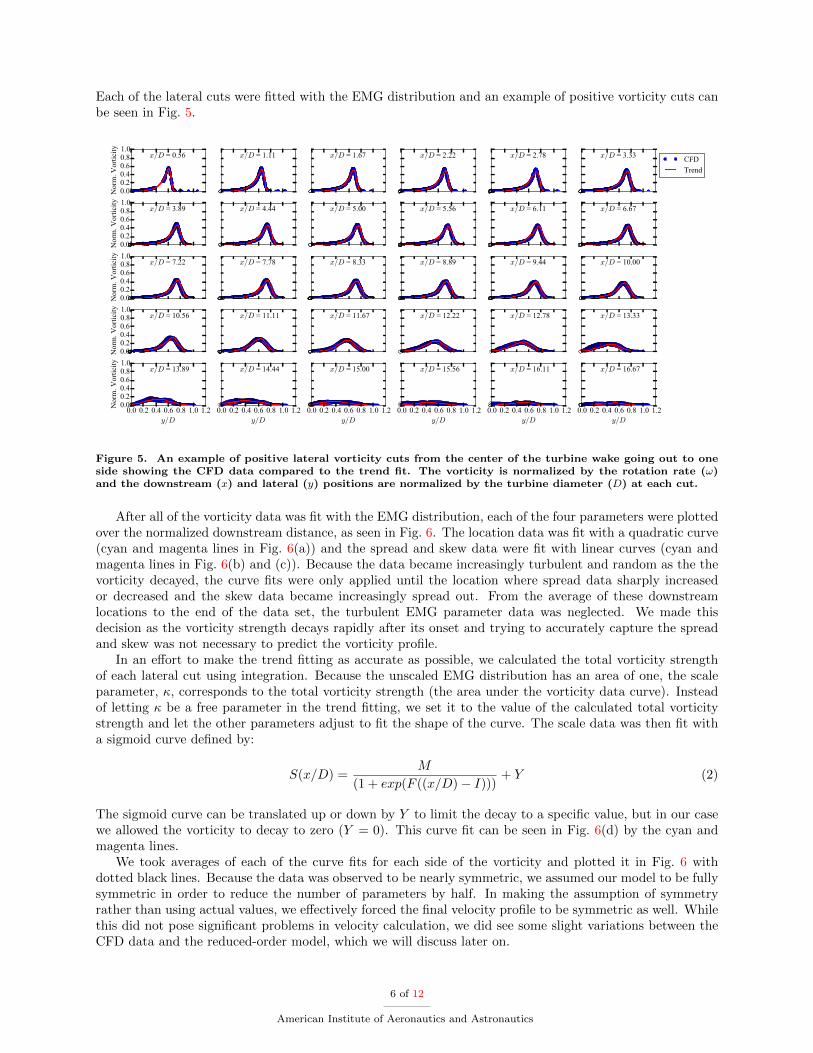
vorticity comes to a maximum value at the center of the stream and then decays away quickly. To analyzethis behavior numerically, we took 30 lateral cuts over the length of the domain, separated the cuts intopositive and negative vorticity sections, and trend fitted each half separately with probabilistic distributions(see Fig. 4 for a representation of this process). To generalize the results for all turbines, both the lateraland downstream distances were normalized by the turbine diameter and the vorticity was normalized by theturbine’s rotation rate.

x

y γ

Lateral Cuts

Figure 4. The lateral vorticity cuts made to analyze the vorticity data numerically seen in orange. Anexaggerated representation of the vorticity distribution is shown with the gray lines. Each of the cuts weresplit into two sections for analysis based on where the vorticity changed sign (negative to positive) whichwas roughly at the center line. The downstream (x) and lateral (y) positions are normalized by the turbinediameter (D) and the vorticity is normalized by the rotation rate (ω).

After exploring several different skewed probabilistic distributions, such as the skewed normal and Weibulldistributions, we found that the best fit was attained using the exponentially modified Gaussian (EMG)distribution. This distribution is defined by four parameters: the location (ξ; the position of the peak), thespread (ν; how wide or narrow the peak was), the skew (α; amount of skewness of the distribution), andthe scale (κ; how high the peak reached). These parameters were used to calculate the vorticity strength(γ(y/D)) as a function of normalized lateral position (y/D) in the equation:

γ(y/D) = κ

[α

2exp

(α2

(2ξ + αν2 − 2(y/D)

))erf

(ξ + αν2 − (y/D)√

2ν

)](1)

5 of 12

American Institute of Aeronautics and Astronautics

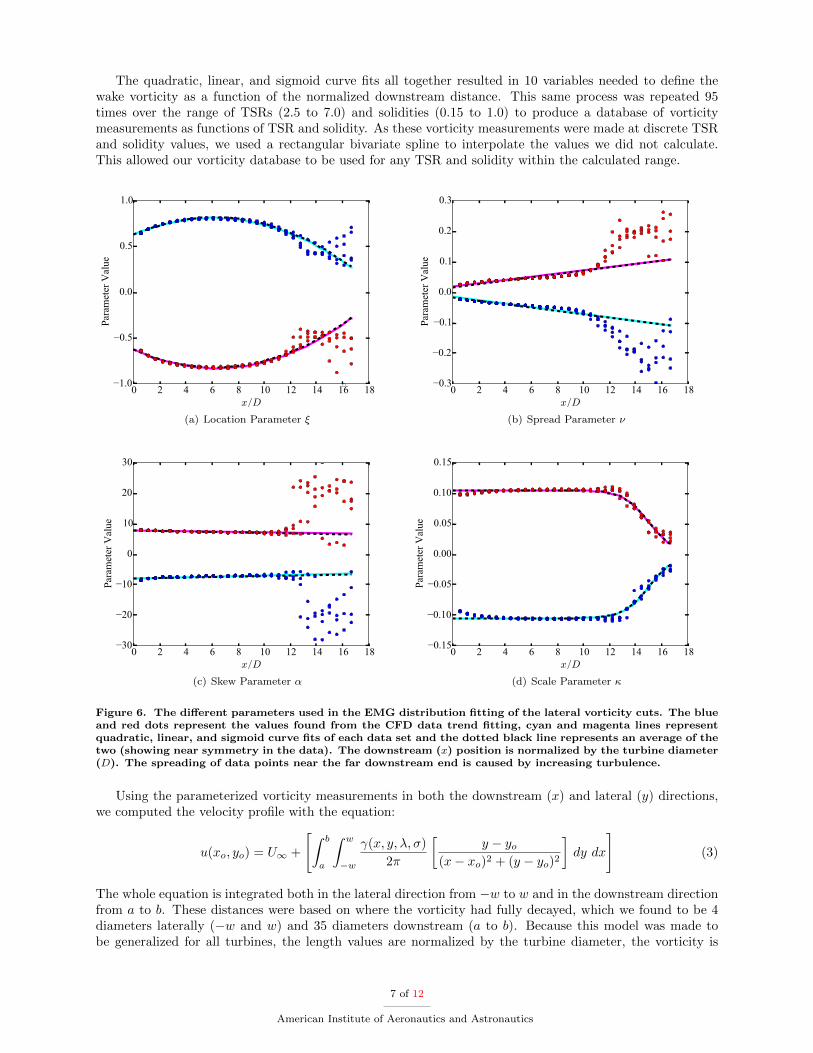
Each of the lateral cuts were fitted with the EMG distribution and an example of positive vorticity cuts canbe seen in Fig. 5.

0.00.20.40.60.81.0

Nor

m. V

ortic

ity

x/D = 0.56 x/D = 1.11 x/D = 1.67 x/D = 2.22 x/D = 2.78 x/D = 3.33 CFDTrend

0.00.20.40.60.81.0

Nor

m. V

ortic

ity

x/D = 3.89 x/D = 4.44 x/D = 5.00 x/D = 5.56 x/D = 6.11 x/D = 6.67

0.00.20.40.60.81.0

Nor

m. V

ortic

ity

x/D = 7.22 x/D = 7.78 x/D = 8.33 x/D = 8.89 x/D = 9.44 x/D = 10.00

0.00.20.40.60.81.0

Nor

m. V

ortic

ity

x/D = 10.56 x/D = 11.11 x/D = 11.67 x/D = 12.22 x/D = 12.78 x/D = 13.33

0.0 0.2 0.4 0.6 0.8 1.0 1.2y/D

0.00.20.40.60.81.0

Nor

m. V

ortic

ity

x/D = 13.89

0.0 0.2 0.4 0.6 0.8 1.0 1.2y/D

x/D = 14.44

0.0 0.2 0.4 0.6 0.8 1.0 1.2y/D

x/D = 15.00

0.0 0.2 0.4 0.6 0.8 1.0 1.2y/D

x/D = 15.56

0.0 0.2 0.4 0.6 0.8 1.0 1.2y/D

x/D = 16.11

0.0 0.2 0.4 0.6 0.8 1.0 1.2y/D

x/D = 16.67

Figure 5. An example of positive lateral vorticity cuts from the center of the turbine wake going out to oneside showing the CFD data compared to the trend fit. The vorticity is normalized by the rotation rate (ω)and the downstream (x) and lateral (y) positions are normalized by the turbine diameter (D) at each cut.

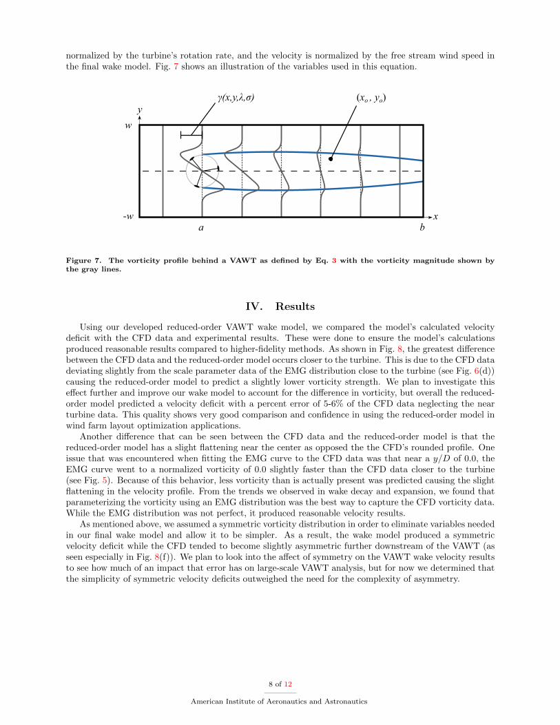
After all of the vorticity data was fit with the EMG distribution, each of the four parameters were plottedover the normalized downstream distance, as seen in Fig. 6. The location data was fit with a quadratic curve(cyan and magenta lines in Fig. 6(a)) and the spread and skew data were fit with linear curves (cyan andmagenta lines in Fig. 6(b) and (c)). Because the data became increasingly turbulent and random as the thevorticity decayed, the curve fits were only applied until the location where spread data sharply increasedor decreased and the skew data became increasingly spread out. From the average of these downstreamlocations to the end of the data set, the turbulent EMG parameter data was neglected. We made thisdecision as the vorticity strength decays rapidly after its onset and trying to accurately capture the spreadand skew was not necessary to predict the vorticity profile.

In an effort to make the trend fitting as accurate as possible, we calculated the total vorticity strengthof each lateral cut using integration. Because the unscaled EMG distribution has an area of one, the scaleparameter, κ, corresponds to the total vorticity strength (the area under the vorticity data curve). Insteadof letting κ be a free parameter in the trend fitting, we set it to the value of the calculated total vorticitystrength and let the other parameters adjust to fit the shape of the curve. The scale data was then fit witha sigmoid curve defined by:

S(x/D) =M

(1 + exp(F ((x/D)− I)))+ Y (2)

The sigmoid curve can be translated up or down by Y to limit the decay to a specific value, but in our casewe allowed the vorticity to decay to zero (Y = 0). This curve fit can be seen in Fig. 6(d) by the cyan andmagenta lines.

We took averages of each of the curve fits for each side of the vorticity and plotted it in Fig. 6 withdotted black lines. Because the data was observed to be nearly symmetric, we assumed our model to be fullysymmetric in order to reduce the number of parameters by half. In making the assumption of symmetryrather than using actual values, we effectively forced the final velocity profile to be symmetric as well. Whilethis did not pose significant problems in velocity calculation, we did see some slight variations between theCFD data and the reduced-order model, which we will discuss later on.

6 of 12

American Institute of Aeronautics and Astronautics

The quadratic, linear, and sigmoid curve fits all together resulted in 10 variables needed to define thewake vorticity as a function of the normalized downstream distance. This same process was repeated 95times over the range of TSRs (2.5 to 7.0) and solidities (0.15 to 1.0) to produce a database of vorticitymeasurements as functions of TSR and solidity. As these vorticity measurements were made at discrete TSRand solidity values, we used a rectangular bivariate spline to interpolate the values we did not calculate.This allowed our vorticity database to be used for any TSR and solidity within the calculated range.

0 2 4 6 8 10 12 14 16 18x/D

1.0

0.5

0.0

0.5

1.0

Para

met

er V

alue

(a) Location Parameter ξ

0 2 4 6 8 10 12 14 16 18x/D

0.3

0.2

0.1

0.0

0.1

0.2

0.3

Para

met

er V

alue

(b) Spread Parameter ν

0 2 4 6 8 10 12 14 16 18x/D

30

20

10

0

10

20

30

Para

met

er V

alue

(c) Skew Parameter α

0 2 4 6 8 10 12 14 16 18x/D

0.15

0.10

0.05

0.00

0.05

0.10

0.15

Para

met

er V

alue

(d) Scale Parameter κ

Figure 6. The different parameters used in the EMG distribution fitting of the lateral vorticity cuts. The blueand red dots represent the values found from the CFD data trend fitting, cyan and magenta lines representquadratic, linear, and sigmoid curve fits of each data set and the dotted black line represents an average of thetwo (showing near symmetry in the data). The downstream (x) position is normalized by the turbine diameter(D). The spreading of data points near the far downstream end is caused by increasing turbulence.

Using the parameterized vorticity measurements in both the downstream (x) and lateral (y) directions,we computed the velocity profile with the equation:

u(xo, yo) = U∞ +

[∫ b

a

∫ w

−w

γ(x, y, λ, σ)

2π

[y − yo

(x− xo)2 + (y − yo)2

]dy dx

](3)

The whole equation is integrated both in the lateral direction from −w to w and in the downstream directionfrom a to b. These distances were based on where the vorticity had fully decayed, which we found to be 4diameters laterally (−w and w) and 35 diameters downstream (a to b). Because this model was made tobe generalized for all turbines, the length values are normalized by the turbine diameter, the vorticity is

7 of 12

American Institute of Aeronautics and Astronautics

normalized by the turbine’s rotation rate, and the velocity is normalized by the free stream wind speed inthe final wake model. Fig. 7 shows an illustration of the variables used in this equation.

(xo , yo)

a b

w

-w x

yγ(x,y,λ,σ)

γ

λσ

λσ

λσ

λσ

Figure 7. The vorticity profile behind a VAWT as defined by Eq. 3 with the vorticity magnitude shown bythe gray lines.

IV. Results

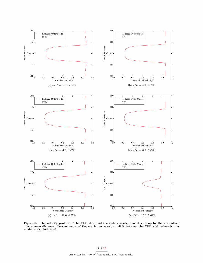
Using our developed reduced-order VAWT wake model, we compared the model’s calculated velocitydeficit with the CFD data and experimental results. These were done to ensure the model’s calculationsproduced reasonable results compared to higher-fidelity methods. As shown in Fig. 8, the greatest differencebetween the CFD data and the reduced-order model occurs closer to the turbine. This is due to the CFD datadeviating slightly from the scale parameter data of the EMG distribution close to the turbine (see Fig. 6(d))causing the reduced-order model to predict a slightly lower vorticity strength. We plan to investigate thiseffect further and improve our wake model to account for the difference in vorticity, but overall the reduced-order model predicted a velocity deficit with a percent error of 5-6% of the CFD data neglecting the nearturbine data. This quality shows very good comparison and confidence in using the reduced-order model inwind farm layout optimization applications.

Another difference that can be seen between the CFD data and the reduced-order model is that thereduced-order model has a slight flattening near the center as opposed the the CFD’s rounded profile. Oneissue that was encountered when fitting the EMG curve to the CFD data was that near a y/D of 0.0, theEMG curve went to a normalized vorticity of 0.0 slightly faster than the CFD data closer to the turbine(see Fig. 5). Because of this behavior, less vorticity than is actually present was predicted causing the slightflattening in the velocity profile. From the trends we observed in wake decay and expansion, we found thatparameterizing the vorticity using an EMG distribution was the best way to capture the CFD vorticity data.While the EMG distribution was not perfect, it produced reasonable velocity results.

As mentioned above, we assumed a symmetric vorticity distribution in order to eliminate variables neededin our final wake model and allow it to be simpler. As a result, the wake model produced a symmetricvelocity deficit while the CFD tended to become slightly asymmetric further downstream of the VAWT (asseen especially in Fig. 8(f)). We plan to look into the affect of symmetry on the VAWT wake velocity resultsto see how much of an impact that error has on large-scale VAWT analysis, but for now we determined thatthe simplicity of symmetric velocity deficits outweighed the need for the complexity of asymmetry.

8 of 12

American Institute of Aeronautics and Astronautics

0.0 0.2 0.4 0.6 0.8 1.0 1.2Normalized Velocity

2D

1D

Center

1D

2D

Late

ral D

ista

nce

Reduced-Order ModelCFD

(a) x/D = 2.0; 15.54%

0.0 0.2 0.4 0.6 0.8 1.0 1.2Normalized Velocity

2D

1D

Center

1D

2D

Late

ral D

ista

nce

Reduced-Order ModelCFD

(b) x/D = 4.0; 9.97%

0.0 0.2 0.4 0.6 0.8 1.0 1.2Normalized Velocity

2D

1D

Center

1D

2D

Late

ral D

ista

nce

Reduced-Order ModelCFD

(c) x/D = 6.0; 6.27%

0.0 0.2 0.4 0.6 0.8 1.0 1.2Normalized Velocity

2D

1D

Center

1D

2D

Late

ral D

ista

nce

Reduced-Order ModelCFD

(d) x/D = 8.0; 5.29%

0.0 0.2 0.4 0.6 0.8 1.0 1.2Normalized Velocity

2D

1D

Center

1D

2D

Late

ral D

ista

nce

Reduced-Order ModelCFD

(e) x/D = 10.0; 4.57%

0.0 0.2 0.4 0.6 0.8 1.0 1.2Normalized Velocity

2D

1D

Center

1D

2D

Late

ral D

ista

nce

Reduced-Order ModelCFD

(f) x/D = 15.0; 5.62%

Figure 8. The velocity profiles of the CFD data and the reduced-order model split up by the normalizeddownstream distance. Percent error of the maximum velocity deficit between the CFD and reduced-ordermodel is also indicated.

9 of 12

American Institute of Aeronautics and Astronautics

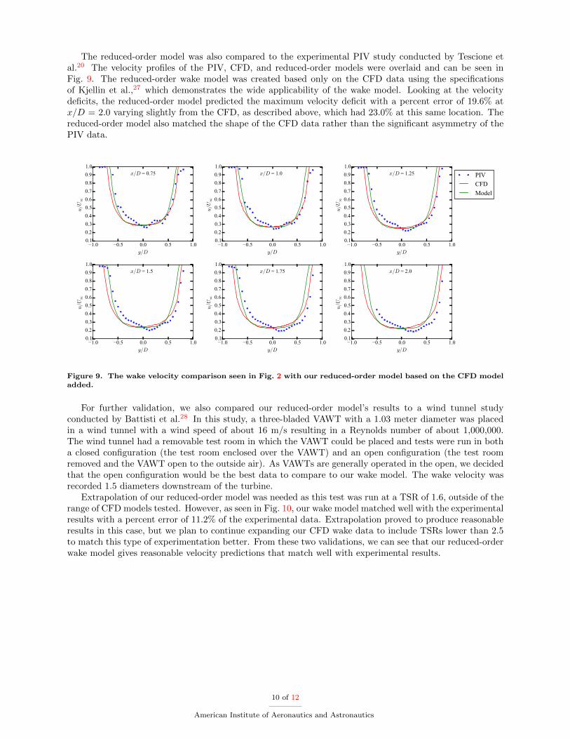
The reduced-order model was also compared to the experimental PIV study conducted by Tescione etal.20 The velocity profiles of the PIV, CFD, and reduced-order models were overlaid and can be seen inFig. 9. The reduced-order wake model was created based only on the CFD data using the specificationsof Kjellin et al.,27 which demonstrates the wide applicability of the wake model. Looking at the velocitydeficits, the reduced-order model predicted the maximum velocity deficit with a percent error of 19.6% atx/D = 2.0 varying slightly from the CFD, as described above, which had 23.0% at this same location. Thereduced-order model also matched the shape of the CFD data rather than the significant asymmetry of thePIV data.

1.0 0.5 0.0 0.5 1.0y/D

0.10.20.30.40.50.60.70.80.91.0

u/U∞

x/D = 0.75

1.0 0.5 0.0 0.5 1.0y/D

0.10.20.30.40.50.60.70.80.91.0

u/U∞

x/D = 1.0

1.0 0.5 0.0 0.5 1.0y/D

0.10.20.30.40.50.60.70.80.91.0

u/U∞

x/D = 1.25 PIVCFDModel

1.0 0.5 0.0 0.5 1.0y/D

0.10.20.30.40.50.60.70.80.91.0

u/U

∞

x/D = 1.5

1.0 0.5 0.0 0.5 1.0y/D

0.10.20.30.40.50.60.70.80.91.0

u/U

∞

x/D = 1.75

1.0 0.5 0.0 0.5 1.0y/D

0.10.20.30.40.50.60.70.80.91.0

u/U

∞

x/D = 2.0

Figure 9. The wake velocity comparison seen in Fig. 2 with our reduced-order model based on the CFD modeladded.

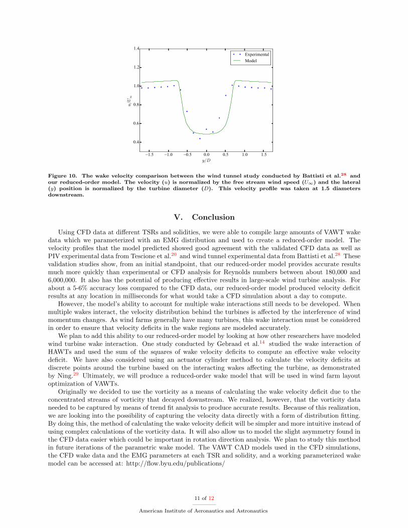
For further validation, we also compared our reduced-order model’s results to a wind tunnel studyconducted by Battisti et al.28 In this study, a three-bladed VAWT with a 1.03 meter diameter was placedin a wind tunnel with a wind speed of about 16 m/s resulting in a Reynolds number of about 1,000,000.The wind tunnel had a removable test room in which the VAWT could be placed and tests were run in botha closed configuration (the test room enclosed over the VAWT) and an open configuration (the test roomremoved and the VAWT open to the outside air). As VAWTs are generally operated in the open, we decidedthat the open configuration would be the best data to compare to our wake model. The wake velocity wasrecorded 1.5 diameters downstream of the turbine.

Extrapolation of our reduced-order model was needed as this test was run at a TSR of 1.6, outside of therange of CFD models tested. However, as seen in Fig. 10, our wake model matched well with the experimentalresults with a percent error of 11.2% of the experimental data. Extrapolation proved to produce reasonableresults in this case, but we plan to continue expanding our CFD wake data to include TSRs lower than 2.5to match this type of experimentation better. From these two validations, we can see that our reduced-orderwake model gives reasonable velocity predictions that match well with experimental results.

10 of 12

American Institute of Aeronautics and Astronautics

1.5 1.0 0.5 0.0 0.5 1.0 1.5y/D

0.4

0.6

0.8

1.0

1.2

1.4

u/U∞

ExperimentalModel

Figure 10. The wake velocity comparison between the wind tunnel study conducted by Battisti et al.28 andour reduced-order model. The velocity (u) is normalized by the free stream wind speed (U∞) and the lateral(y) position is normalized by the turbine diameter (D). This velocity profile was taken at 1.5 diametersdownstream.

V. Conclusion

Using CFD data at different TSRs and solidities, we were able to compile large amounts of VAWT wakedata which we parameterized with an EMG distribution and used to create a reduced-order model. Thevelocity profiles that the model predicted showed good agreement with the validated CFD data as well asPIV experimental data from Tescione et al.20 and wind tunnel experimental data from Battisti et al.28 Thesevalidation studies show, from an initial standpoint, that our reduced-order model provides accurate resultsmuch more quickly than experimental or CFD analysis for Reynolds numbers between about 180,000 and6,000,000. It also has the potential of producing effective results in large-scale wind turbine analysis. Forabout a 5-6% accuracy loss compared to the CFD data, our reduced-order model produced velocity deficitresults at any location in milliseconds for what would take a CFD simulation about a day to compute.

However, the model’s ability to account for multiple wake interactions still needs to be developed. Whenmultiple wakes interact, the velocity distribution behind the turbines is affected by the interference of windmomentum changes. As wind farms generally have many turbines, this wake interaction must be consideredin order to ensure that velocity deficits in the wake regions are modeled accurately.

We plan to add this ability to our reduced-order model by looking at how other researchers have modeledwind turbine wake interaction. One study conducted by Gebraad et al.14 studied the wake interaction ofHAWTs and used the sum of the squares of wake velocity deficits to compute an effective wake velocitydeficit. We have also considered using an actuator cylinder method to calculate the velocity deficits atdiscrete points around the turbine based on the interacting wakes affecting the turbine, as demonstratedby Ning.29 Ultimately, we will produce a reduced-order wake model that will be used in wind farm layoutoptimization of VAWTs.

Originally we decided to use the vorticity as a means of calculating the wake velocity deficit due to theconcentrated streams of vorticity that decayed downstream. We realized, however, that the vorticity dataneeded to be captured by means of trend fit analysis to produce accurate results. Because of this realization,we are looking into the possibility of capturing the velocity data directly with a form of distribution fitting.By doing this, the method of calculating the wake velocity deficit will be simpler and more intuitive instead ofusing complex calculations of the vorticity data. It will also allow us to model the slight asymmetry found inthe CFD data easier which could be important in rotation direction analysis. We plan to study this methodin future iterations of the parametric wake model. The VAWT CAD models used in the CFD simulations,the CFD wake data and the EMG parameters at each TSR and solidity, and a working parameterized wakemodel can be accessed at: http://flow.byu.edu/publications/

11 of 12

American Institute of Aeronautics and Astronautics

References

1Bazilevs, Y., Korobenko, A., Deng, X., Yan, J., Kinzel, M., and Dabiri, J. O., “Fluid-Structure Interaction Modeling ofVertical-Axis Wind Turbines,” Journal of Applied Mechanics, Vol. 81, August 2014.

2Fichaux, N., Wilkes, J., Hulle, F. V., and Cronin, A., “Oceans of Opportunity: Harnessing Europe’s largest domesticenergy resource,” Tech. Rep. 41018647, European Wind Energy Association, September 2009.

3Maples, B., Saur, G., Hand, M., van de Pietermen, R., and Obdam, T., “Installation, Operation, and MaintenanceStrategies to Reduce the Cost of Offshore Wind Energy,” Tech. Rep. NREL/TP-5000-57403, National Renewable EnergyLaboratory, July 2013.

4Dabiri, J. O., Greer, J. R., Koseff, J. R., Moin, P., and Peng, J., “A New Approach To Wind Energy: Opportunities andChallenges,” AIP Conference Proceedings, 2015.

5Sandia National Laboratories, “Offshore use of vertical-axis wind turbines gets closer look,” July 2012.6Sutherland, H. J., Berg, D. E., and Ashwill, T. D., “A Retrospective of VAWT Technology,” Tech. rep., Sandia National

Laboratories, January 2012.7Vermeer, L., Sørensen, J., and Crespo, A., “Wind turbine wake aerodynamics,” Progress in Aerospace Sciences, Vol. 39,

2003, pp. 467–510.8Crespo, A., Hernandez, J., and Frandsen, S., “Survey of Modelling Methods for Wind Turbine Wakes and Wind Farms,”

Wind Energy, Vol. 2, 1999, pp. 1–24.9Sanderse, B., “Aerodynamics of wind turbine wakes,” Tech. Rep. ECN-E09-016, Energy Centre of the Netherlands, 2009.

10Changshui, Z., Guangdong, H., and Jun, W., “A fast algorithm based on the submodular property for optimization ofwind turbine positioning,” Renewable Energy, Vol. 36, 2011, pp. 2951–2958.

11Kusiak, A. and Song, Z., “Design of wind farm layout for maximum wind energy capture,” Renewable Energy, Vol. 35,No. 3, 2010, pp. 685–694.

12Eroglu, Y. and Seckiner, S. U., “Design of wind farm layout using ant colony algorithm,” Renewable Energy, Vol. 44,2014, pp. 53–62.

13Perez, B., Mınguez, R., and Guanche, R., “Offshore Wind Farm Layout Optimization Using Mathematical ProgrammingTechniques,” Renewable Energy, Vol. 53, 2013, pp. 389–399.

14Gebraad, P. M. O., Teeuwisse, F. W., van Wingerden, J. W., Fleming, P. A., Ruben, S. D., Marden, J. R., and Pao,L. Y., “Wind plant power optimization through yaw control using a parametric model for wake effects—a CFD simulationstudy,” Wind Energy, 2014.

15Gebraad, P. M., Thomas, J. J., Ning, A., Fleming, P. A., and Dykes, K., “Maximization of the annual energy productionof wind power plants by optimization of layout and yaw-based wake control,” (in review).

16Fleming, P., Ning, A., Gebraad, P., and Dykes, K., “Wind Plant System Engineering through Optimization of Layoutand Yaw Control,” Wind Energy, March 2015.

17Sheldahl, R. E. and Klimas, P. C., “Aerodynamic Characteristics of Seven Symmetrical Airfoil Sections Through 180-Degree Angle of Attack for Use in Aerodynamic Analysis of Vertical Axis Wind Turbines,” Tech. rep., Sandia National Labo-ratories, Advanced Energy Projects Division 4715, Sandia National Laboratories, Albuquerque, NM 87185, March 1981.

18Sheldahl, R. E., “Comparison of Field and Wind Tunnel Darrieus Wind Turbine Data,” Tech. rep., Sandia NationalLaboratories, January 1981.

19Worstell, M. H., “Aerodynamic Performance of the 17 Meter Diameter Darrieus Wind Turbine,” Tech. rep., SandiaNational Laboratories, September 1978.

20Tescione, G., Ragni, D., He, C., Ferreira, C. S., and van Bussel, G., “Near wake flow analysis of a vertical axis windturbine by stereoscopic particle image velocimetry,” Renewable Energy, Vol. 70, 2014, pp. 47–61.

21Ferreira, C. J. S., The Near Wake of the VAWT: 2D and 3D Views of the VAWT Aerodynamics, Ph.D. thesis, DelftUniversity of Technology, 2009.

22Ferreira, C. S., Madsen, H. A., Barone, M., Roscher, B., Deglaire, P., and Arduin, I., “Comparison of aerodynamic modelfor Vertical Axis Wind Turbines,” Journal of Physics, Vol. 524, 2014.

23He, C., Wake Dynamics Study of an H-type Vertical Axis Wind Turbine, Master’s thesis, Delft University of Technology,August 2013.

24Dixon, K. R., The Near Wake Structure of a Vertical Axis Wind Turbine: Including the Development of a 3D UnsteadyFree-Wake Panel Method for VAWTs, Master’s thesis, Delft University of Technology, April 2008.

25Shamsoddin, S. and Porte-Agel, F., “Large Eddy Simulation of Vertical Axis Wind Turbine Wakes,” Energies, Vol. 7,2014, pp. 8990–8912.

26Whittlesey, R. W., Liska, S., and Dabiri, J. O., “Fish schooling as a basis for vertical axis wind turbine farm design,”Tech. rep., California Institute of Technology, February 2010.

27Kjellin, J., Bulow, F., Eriksson, S., Deglaire, P., Leijon, M., and Bernhoff, H., “Power coefficient measurement on a 12kW straight bladed vertical axis wind turbine,” Renewable Energy, Vol. 36, 2011, pp. 3050–3053.

28Battisti, L., Zanne, L., Dell’Anna, S., Dossena, V., Persico, G., and Paradiso, B., “Aerodynamic Measurements on aVertical Axis Wind Turbine in a Large Scale Wind Tunnel,” Journal of Energy Resources Technology, Vol. 133, September2011.

29Ning, A., “Actuator Cylinder Theory for Multiple Vertical Axis Wind Turbines,” (in review), 2015.

12 of 12

American Institute of Aeronautics and Astronautics