Embed Size (px)
Citation preview
Fast Image Super-resolution Based on In-place Example Regression
Jianchao Yang, Zhe Lin, Scott CohenAdobe Research
345 Park Avenue, San Jose, CA 95110{jiayang, zlin, scohen}@adobe.com
Abstract
We propose a fast regression model for practical sin-gle image super-resolution based on in-place examples, byleveraging two fundamental super-resolution approaches—learning from an external database and learning from self-examples. Our in-place self-similarity refines the recentlyproposed local self-similarity by proving that a patch in theupper scale image have good matches around its origin lo-cation in the lower scale image. Based on the in-place ex-amples, a first-order approximation of the nonlinear map-ping function from low- to high-resolution image patchesis learned. Extensive experiments on benchmark and real-world images demonstrate that our algorithm can producenatural-looking results with sharp edges and preserved finedetails, while the current state-of-the-art algorithms areprone to visual artifacts. Furthermore, our model can eas-ily extend to deal with noise by combining the regressionresults on multiple in-place examples for robust estimation.The algorithm runs fast and is particularly useful for prac-tical applications, where the input images typically containdiverse textures and they are potentially contaminated bynoise or compression artifacts.
1. Introduction
Single image super-resolution aims at generating a high-
resolution image from one low-resolution input. The prob-
lem is dramatically under-constrained, and thus it has to rely
on some strong image priors for robust estimation. Such im-
age priors range from simple analytical “smoothness” priors
to more sophisticated statistical priors learned from natural
images [16, 5, 7, 19, 10].
For image upscaling, the most popular methods are those
based on analytical interpolations, e.g., bicubic interpola-
tion, with the image “smoothness” assumption. As im-
ages contain strong discontinuities, such as edges and cor-
ners, the simple “smoothness” prior will result in ring-
ing, jaggy and blurring artifacts. Therefore, more sophis-
ticated statistical priors learned from natural images are ex-
plored [5, 3, 13, 15]. However, even though natural im-
ages are sparse signals, trying to capture their rich charac-
teristics with only a few parameters is impossible. Alterna-
tively, example-based nonparametric methods [7, 14, 2, 17]
were used to predict the missing frequency band of the up-
sampled image, by relating the image pixels at two spatial
scales using a universal set of training example patch pairs.
Typically, a huge set of training patches are needed, result-
ing in excessively heavy computation cost. Taking one step
further, Yang et al. [19, 18] proposed to use sparse linear
combinations to recover the missing high-frequency band,
allowing a much more compact dictionary model based on
sparse coding.
Some recent studies show that images generally possess
a great amount of self-similarities, i.e., local image struc-
tures tend to recur within and across different image scales
[4, 1, 21], and image super-resolution can be regularized
based on these self-similar examples instead of some exter-
nal database [4, 9, 6]. In particular, Glasner et al. [9] use
self-examples within and across multiple image scales to
regularize the otherwise ill-posed classical super-resolution
scheme. Freedman and Fattal [6] extend the example-based
super-resolution framework with self-examples and itera-
tively upscale the image. They show that the local self-
similarity assumption for natural images holds better for
small upscaling factors and the patch search can be con-
ducted in a restricted local region, allowing a very fast prac-
tical implementation.
In this paper, we refine the local self-similarity [6, 21] by
in-place self-similarity, by proving that, for a query patch
in the upper scale image, patch matching can be restricted
to its origin location in the lower scale image. Based on
these in-place examples, we learn a robust first-order ap-
proximation of the nonlinear mapping function from low-
to high-resolution image patches. Compared with the state-
of-the-art methods [9, 18, 6], our algorithm runs very fast
and can produce more natural structures, thereby it is bet-
ter at handling real applications, where the input images
contain complex structures and diverse textures and they
are potentially contaminated by sensor noise (e.g, cellphone
2013 IEEE Conference on Computer Vision and Pattern Recognition
1063-6919/13 $26.00 © 2013 IEEE
DOI 10.1109/CVPR.2013.141
1057
2013 IEEE Conference on Computer Vision and Pattern Recognition
1063-6919/13 $26.00 © 2013 IEEE
DOI 10.1109/CVPR.2013.141
1057
2013 IEEE Conference on Computer Vision and Pattern Recognition
1063-6919/13 $26.00 © 2013 IEEE
DOI 10.1109/CVPR.2013.141
1057
2013 IEEE Conference on Computer Vision and Pattern Recognition
1063-6919/13 $26.00 © 2013 IEEE
DOI 10.1109/CVPR.2013.141
1059
2013 IEEE Conference on Computer Vision and Pattern Recognition
1063-6919/13 $26.00 © 2013 IEEE
DOI 10.1109/CVPR.2013.141
1059
cameras) or compression artifacts (e.g, internet images). In
summary, this paper makes the following contributions.
1. We propose a new fast super-resolution algorithm
based on regression on in-place examples, which,
for the first time, leverages the two fundamental
super-resolution approaches of learning from external-
examples and learning from self-examples.
2. We prove that patch matching across different image
scales with small scaling factors is in-place, which re-
fines and validates the recently proposed local self-
similarity theoretically.
3. We can easily extend our algorithm to handle noisy in-
put images by combining regression results on multi-
ple in-place examples. The algorithm runs very fast
and is particularly useful for real applications.
The remainder of the paper is organized as follows. Sec-
tion 2 introduces the notations we use. Section 3 presents
our robust regression model for super-resolution. Section 4
presents our algorithm implementation details and results
on both synthetic and real-world images. Finally, Section 5
concludes our paper.
2. Preliminaries and NotationsThis work focuses on upscaling an input image X0
which contains some high-frequency content that we can
borrow for image super-resolution, i.e., X0 is a sharp image
but with unsatisfactory pixel resolution.1 In the following,
we use X0 and X to denote the input and output (by s×) im-
ages, and Y0 and Y their low-frequency bands, respectively.
That is, Y0 (Y ) has the same spatial dimension as X0 (X),
but is missing the high-frequency content. We use bolded
lower case x0 and x to denote a×a image patches sampled
from X0 and X , respectively, and y0 and y to denote a× aimage patches sampled from Y0 and Y , respectively. y0 and
y are thus referred as low-resolution image patches because
they are missing high-frequency components, while x0 and
x are referred as their high-resolution counterparts. Plain
lower case (x, y) and (p, q) denote coordinates in the 2D
image plane.
3. Regression on In-place ExamplesIn this section, we present our super-resolution algorithm
based on learning the in-place example regression by refer-
ring to an external database.
3.1. The Image Super-resolution Scheme
Similar to [6], we first describe our overall image upscal-
ing scheme in Figure 1, which is based on in-place exam-ples and first-order regression that will be discussed shortly.
1This is the implicit assumption of most previous example-based ap-
proaches.
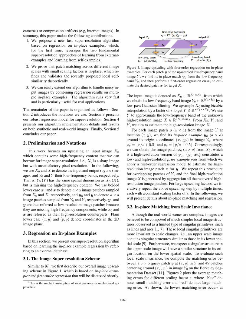
Figure 1. Image upscaling with first-order regression on in-place
examples. For each patch y of the upsampled low-frequency band
image Y , we find its in-place match y0 from the low-frequency
band Y0, and then perform a first-order regression on x0 to esti-
mate the desired patch x for target X .
The input image is denoted as X0 ∈ RK1×K2 , from which
we obtain its low-frequency band image Y0 ∈ RK1×K2 by a
low-pass Gaussian filtering. We upsample X0 using bicubic
interpolation by a factor of s to get Y ∈ RsK1×sK2 . We use
Y to approximate the low-frequency band of the unknown
high-resolution image X ∈ RsK1×sK2 . From X0, Y0, and
Y , we aim to estimate the high-resolution image X .
For each image patch y (a × a) from the image Y at
location (x, y), we find its in-place example y0 (a × a)
around its origin coordinates (xr, yr) in image Y0, where
xr = �x/s+ 0.5� and yr = �y/s+ 0.5�. Correspondingly,
we can obtain the image patch x0 (a × a) from X0, which
is a high-resolution version of y0. {y0,x0} constitutes a
low- and high-resolution prior example pair from which we
apply a first-order regression model to estimate the high-
resolution image patch x for y. We repeat this procedure
for overlapping patches of Y , and the final high-resolution
image X is generated by aggregation all the recovered high-
resolution image patches. For large upscaling factors, we it-
eratively repeat the above upscaling step by multiple times,
each with a constant scaling factor of s. In the following, we
will present details about in-place matching and regression.
3.2. In-place Matching from Scale Invariance
Although the real-world scenes are complex, images are
believed to be composed of much simpler local image struc-
tures, observed as a limited type of singular primitives, such
as lines and arcs [1, 7]. These local singular primitives are
more invariant to scale changes, i.e., an upper scale image
contains singular structures similar to those in its lower spa-
tial scale [9]. Furthermore, we expect a singular structure in
the upper scale image will have a similar structure in its ori-
gin location on the lower spatial scale. To evaluate such
local scale invariance, we compute the matching error be-
tween a 5 × 5 query patch y at (x, y) in Y and 49 patches
centering around (xr, yr) in image Y0 on the Berkeley Seg-
mentation Dataset [11]. Figures 2 plots the average match-
ing errors for different scaling factor s, where “blue” de-
notes small matching error and “red” denotes large match-
ing error. As shown, the lowest matching error occurs at
10581058105810601060

1 2 3 4 5 6 7
1
2
3
4
5
6
7
1 2 3 4 5 6 7
1
2
3
4
5
6
7
1 2 3 4 5 6 7
1
2
3
4
5
6
7
1 2 3 4 5 6 7
1
2
3
4
5
6
7
s = 1.25 s = 1.5 s = 2 s = 3
Figure 2. Matching errors of each patch y in an upper-scale image
with its in-place neighbors in the lower-scale image for different
scaling factors.
center (xr, yr) on average, and the smaller the scaling fac-
tor, the lower the matching error, and the more concentrated
the area with lower matching error. Therefore, for a small
scaling factor, finding a similar match for a query patch
y could be extremely localized on Y0. For image upscal-
ing, we want to preserve the high-frequency information for
the singular primitives. The local scale invariance indicates
that we could efficiently find a similar example y0 for y,
and thus the corresponding high-resolution patch x0, from
which we can infer the high-frequency information of y.
Formally, we refine this local self-similarity in the follow-
ing proposition (proof in the appendix).
Proposition. For each patch y of size a × a (a > 2) fromupsampled image Y at location (x, y), containing only onesingular primitive, the location (x0, y0) of a close match y0
in Y0 for y will be at most one pixel away from y’s originlocation (x/s, y/s) on Y0, i.e., |x0 − x/s| < 1 and |y0 −y/s| < 1, given the scaling factor s < a/(a− 2).
Therefore, the search region for y on Y0 is in-place, and
y0 is called an in-place example for patch y. Based on the
in-place example pair {y0,x0}, we perform a first-order
regression to estimate the high-resolution information for
patch y in the following section.
3.3. In-place Example Regression
The patch-based single image super-resolution problem
can be viewed as a regression problem, i.e., finding a map-
ping function f from the low-resolution patch space to the
target high-resolution patch space. However, learning this
regression function turns out to be extremely difficult due to
the ill-posed nature of super-resolution; proper regulariza-
tions or good image priors are need to constrain the solution
space. From the above analysis, the in-place example pair
{y0,x0} serves as a good prior example pair for inferring
the high-resolution version of y. Assuming some smooth-
ness on the mapping function f 2, we have the following
Taylor expansion:
x =f(y) = f(y0 + y − y0)
=f(y0) +∇fT (y0)(y − y0) + o(‖y − y0‖22)≈x0 +∇fT (y0)(y − y0),
(1)
2This is a reasonable assumption, as one will not expect a dramatic
change in the high-resolution patch for a minor change in the low-
resolution image patch, especially in the case of small scaling factors.
which is based on the facts that x0 = f(y0) and y is close
to y0.3 The equation is a first-order approximation for the
mapping function f . Instead of learning f directly, we learn
the derivative function ∇f , which is better constrained by
the in-place example pairs and should be simpler.
For simplicity, we approximate the function ∇f as a
piece-wise constant function by learning the function val-
ues on a set of anchor points {c1, ..., cn} sampled from the
low-resolution patch space. Given a set of training example
pairs {yi,xi}mi=1 and their corresponding prior in-place ex-
ample pairs {y0i,x0i}mi=14, we can learn the function ∇f
on the n anchor points by
min{∇f(cj)}nj=1
m∑
i=1
‖xi − x0i −∇f(ci∗)(yi − y0i)‖22, (2)
where ci∗ is the nearest anchor point to y0i. The above
optimization can be easily solved by least squares. With
the function values on the anchor points learned, for any
patch y, we first search its in-place example pair {y0,x0},find∇f(y0) based on its nearest anchor point, and then use
the first order approximation to compute the high-resolution
patch x.
Discussions In previous example-based super-resolution
works [7, 6], the high-resolution image patch x is obtained
by transferring the high-frequency component from the best
prior example pair {y0,x0} to the low-resolution image
patch y, i.e.,
x = y + (x0 − y0) = x0 + (y − y0). (3)
Instead of high frequency transfer, why not using x0 di-
rectly as the estimation of x? Note that x = x0+x−x0 =x0 +�x. The above equation simply uses �y = y − y0
to approximate �x for error compensation, which is rea-
sonable because �y is a blurred version of �x. Compar-
ing the above equation with Eqn. 1, we can see that high-
frequency component transfer is an approximate of the first-
order regression model by setting the derivative function
∇f to be the identity matrix. By learning the derivative
function, we actually learn a set of adaptive linear sharpen-
ing filters that sharpens �y to approximate �x, and thus
our approximation to the mapping function f is more accu-
rate. On the other hand, using x0 directly as an estima-
tion for x can be seen as a zero-order approximation of
f from Eqn. 1, which does not account for error compen-
sation and thus has larger approximation errors. Figure 3
shows the super-resolution comparisons between zero- and
our first-order approximations. The results are obtained by
recovering overlapping low-resolution image patches which
3Here, x, y, x0 and y0 are in their vectorized form4The prior in-place example pairs are found based on {yi}mi=1 only as
discussed before.
10591059105910611061

Figure 3. Example-based super-resolution results (2×). Left:
zero-order approximation; right: our first-order regression.
are later averaged at the same pixel locations. Because the
zero-order approximation has large approximation errors,
the overlapping pixel predictions do not agree with each
other. As a result, averaging them will severely blur the im-
age. Our first-order approximation is much more accurate
and thus preserves the image details.
Motivated by locally linear embedding [12], Chang et al.
[2] generalized the framework of [7] by proposing a locally
linear model to directly learn the mapping function f . How-
ever, the algorithm still requires a large number of training
examples in order to approximate f well, resulting in expen-
sive computations for practical applications. In addition, as
shown in [19], Chang’s algorithm is very sensitive to noise.
3.4. Aggregating In-place Example Regressions
Due to the discrete resampling process in downsampling
and upsampling for small scaling factors (non-dyadic), one
typically cannot find the exact in-place example; instead,
one will find multiple approximate in-place examples for yin the neighborhood of (xr, yr), which contains at most 9
patches. To reduce the regression variance, we can perform
regression on each of them and combine the results by a
weighted average. Given the in-place prior example pairs
{y0i,x0i}9i=1 for y, we have
x =9∑
i=1
wi
{x0i +∇fT (y0i)(y − y0i)
}, (4)
where wi = 1/z · exp (−‖y − y0i‖22/2σ2)
with z the nor-
malization factor. The above aggregated regression on mul-
tiple in-place examples is of important practical values. In
real image super-resolution scenarios, the test image might
be contaminated by noise, e.g., photos shot by mobile cam-
eras, or by compression artifacts, e.g., images from the in-
ternet. It is extremely important for the super-resolution al-
gorithm to be robust to such image degradations. By ag-
gregating the multiple regression results, our algorithm can
handle different image degradations well in practical appli-
cations. It is worthy to note that our formulation only uses
regression results on extremely localized in-place examples
in a lower spatial scale, which is different from that of the
non-local means algorithm [1] that operates on raw image
patches in a much larger spatial window at the same spatial
scale.
Table 1. Prediction RMSEs for different approaches on testing
patches and images for one upscaling step (1.5×).
Approaches bicubic zero order transfer regression
testing patches 8.59 14.67 9.34 8.21kid 3.47 4.93 3.45 2.88
barbara 8.31 10.40 8.14 6.87worker 8.44 9.36 7.20 6.29
lena 4.31 5.01 3.66 3.21koala 3.79 5.12 3.59 2.96girl 4.32 5.45 3.97 3.39wall 10.08 11.11 9.09 8.15
3.5. Selective Patch Processing
Natural images typically contain large smooth regions
with sparse discontinuities. Although simple interpolation
methods result in artifacts along the discontinuities, they
perform well on smooth regions. This observation suggests
that we only need to process the textured regions with our
super-resolution model, while leaving the large smooth re-
gions to simple and fast interpolation techniques. To differ-
entiate smooth and textured regions, we do SVD on the gra-
dient matrix of a local image patch, and calculate the singu-
lar values s1 ≥ s2 ≥ 0, which represent the energies in the
dominant local gradient and edge orientation. Specifically,
we use the following two image content metrics defined in
[20] to find the textured regions: R = s1−s2s1+s2
, Q = s1s1−s2s1+s2
,
where R and Q are large for textured regions and small for
smooth regions. Therefore, we can selectively process im-
age patches with center R and Q values larger than some
predefined thresholds, which leads to a speedup of 2 ∼ 3times without compromise in the image quality.
4. Experimental Results
In this section, we evaluate our algorithm on both syn-
thetic test examples used in the super-resolution literature
and real-world test examples. In both cases, our algorithm
can produce compelling results with a practically fast speed.
Parameters We choose patch size a = 5 and iterative
scaling factor s = 1.5 in our experiments, in order to sat-
isfy the in-place matching constraints in the proposition.
The low-frequency band Y of the target high-resolution im-
age is approximated by bicubic interpolation from X0. The
low-frequency band Y0 of the input image X0 is obtained
by a low-pass Gaussian filtering with a standard deviation
of 0.55. The image patches of Y are processed with over-
lapping pixels, which are simply averaged to get the final
result. For clean images, we use the nearest neighbor in-
place example for regression, and for noisy images, we av-
erage all 9 in-place example regressions for robust estima-
tion, where σ is the only tuning parameter to compute wi in
Eqn. 4 depending on the noise level.
10601060106010621062
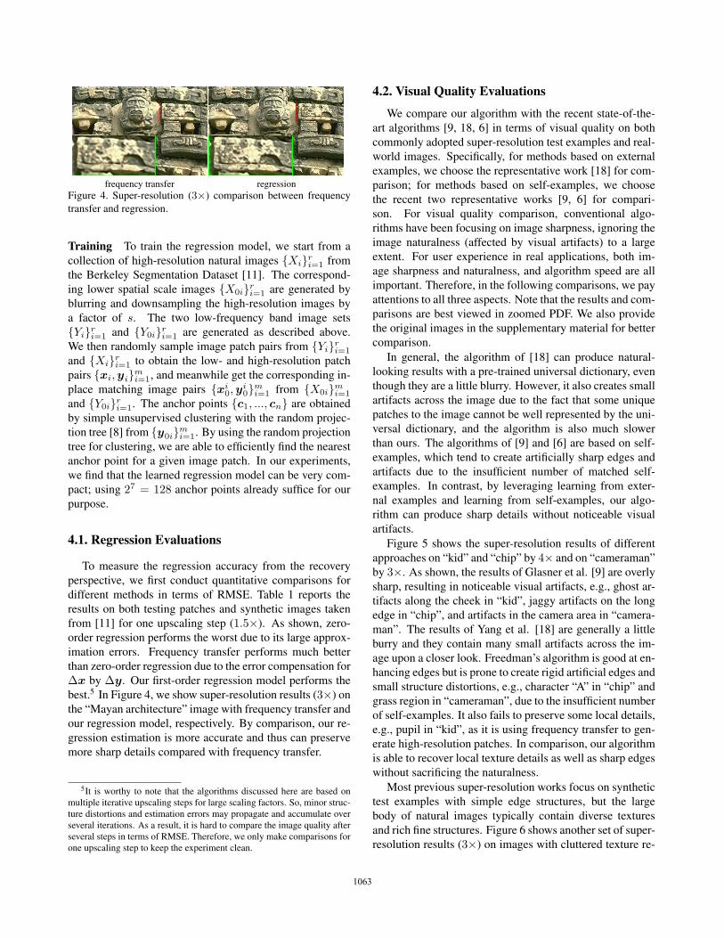
frequency transfer regression
Figure 4. Super-resolution (3×) comparison between frequency
transfer and regression.
Training To train the regression model, we start from a
collection of high-resolution natural images {Xi}ri=1 from
the Berkeley Segmentation Dataset [11]. The correspond-
ing lower spatial scale images {X0i}ri=1 are generated by
blurring and downsampling the high-resolution images by
a factor of s. The two low-frequency band image sets
{Yi}ri=1 and {Y0i}ri=1 are generated as described above.
We then randomly sample image patch pairs from {Yi}ri=1
and {Xi}ri=1 to obtain the low- and high-resolution patch
pairs {xi,yi}mi=1, and meanwhile get the corresponding in-
place matching image pairs {xi0,y
i0}mi=1 from {X0i}mi=1
and {Y0i}ri=1. The anchor points {c1, ..., cn} are obtained
by simple unsupervised clustering with the random projec-
tion tree [8] from {y0i}mi=1. By using the random projection
tree for clustering, we are able to efficiently find the nearest
anchor point for a given image patch. In our experiments,
we find that the learned regression model can be very com-
pact; using 27 = 128 anchor points already suffice for our
purpose.
4.1. Regression Evaluations
To measure the regression accuracy from the recovery
perspective, we first conduct quantitative comparisons for
different methods in terms of RMSE. Table 1 reports the
results on both testing patches and synthetic images taken
from [11] for one upscaling step (1.5×). As shown, zero-
order regression performs the worst due to its large approx-
imation errors. Frequency transfer performs much better
than zero-order regression due to the error compensation for
Δx by Δy. Our first-order regression model performs the
best.5 In Figure 4, we show super-resolution results (3×) on
the “Mayan architecture” image with frequency transfer and
our regression model, respectively. By comparison, our re-
gression estimation is more accurate and thus can preserve
more sharp details compared with frequency transfer.
5It is worthy to note that the algorithms discussed here are based on
multiple iterative upscaling steps for large scaling factors. So, minor struc-
ture distortions and estimation errors may propagate and accumulate over
several iterations. As a result, it is hard to compare the image quality after
several steps in terms of RMSE. Therefore, we only make comparisons for
one upscaling step to keep the experiment clean.
4.2. Visual Quality Evaluations
We compare our algorithm with the recent state-of-the-
art algorithms [9, 18, 6] in terms of visual quality on both
commonly adopted super-resolution test examples and real-
world images. Specifically, for methods based on external
examples, we choose the representative work [18] for com-
parison; for methods based on self-examples, we choose
the recent two representative works [9, 6] for compari-
son. For visual quality comparison, conventional algo-
rithms have been focusing on image sharpness, ignoring the
image naturalness (affected by visual artifacts) to a large
extent. For user experience in real applications, both im-
age sharpness and naturalness, and algorithm speed are all
important. Therefore, in the following comparisons, we pay
attentions to all three aspects. Note that the results and com-
parisons are best viewed in zoomed PDF. We also provide
the original images in the supplementary material for better
comparison.
In general, the algorithm of [18] can produce natural-
looking results with a pre-trained universal dictionary, even
though they are a little blurry. However, it also creates small
artifacts across the image due to the fact that some unique
patches to the image cannot be well represented by the uni-
versal dictionary, and the algorithm is also much slower
than ours. The algorithms of [9] and [6] are based on self-
examples, which tend to create artificially sharp edges and
artifacts due to the insufficient number of matched self-
examples. In contrast, by leveraging learning from exter-
nal examples and learning from self-examples, our algo-
rithm can produce sharp details without noticeable visual
artifacts.
Figure 5 shows the super-resolution results of different
approaches on “kid” and “chip” by 4× and on “cameraman”
by 3×. As shown, the results of Glasner et al. [9] are overly
sharp, resulting in noticeable visual artifacts, e.g., ghost ar-
tifacts along the cheek in “kid”, jaggy artifacts on the long
edge in “chip”, and artifacts in the camera area in “camera-
man”. The results of Yang et al. [18] are generally a little
burry and they contain many small artifacts across the im-
age upon a closer look. Freedman’s algorithm is good at en-
hancing edges but is prone to create rigid artificial edges and
small structure distortions, e.g., character “A” in “chip” and
grass region in “cameraman”, due to the insufficient number
of self-examples. It also fails to preserve some local details,
e.g., pupil in “kid”, as it is using frequency transfer to gen-
erate high-resolution patches. In comparison, our algorithm
is able to recover local texture details as well as sharp edges
without sacrificing the naturalness.
Most previous super-resolution works focus on synthetic
test examples with simple edge structures, but the large
body of natural images typically contain diverse textures
and rich fine structures. Figure 6 shows another set of super-
resolution results (3×) on images with cluttered texture re-
10611061106110631063

Bicubic Glasner et al. [9] Yang et al. [18] Freedman & Fattal [6] Ours
Figure 5. Super-resolution results on “kid” (4×), “chip” (4×) and “Cameraman” (3×). Our algorithm can generate natural-looking results
without noticeable visual artifacts. Results are better viewed in zoomed PDF.
gions. The algorithm in [18] can produce natural looking
results, but the textures are a little blurry with occassional
small artifacts. Freedman and Fattal’s again fails to recover
the fine details and produces many rigid false edges in the
textured regions. Besides images with complex and diverse
structures, we also encounter frequently noisy images in
real applications, e.g., images captured by low cost sensors
are typically contaminated by some amount of sensor noise
and internet images with JPEG compression artifacts. It is
extremely important that the super-resolution algorithm is
robust to such degradations. By averaging the regression re-
sults on multiple in-place self-examples, our algorithm can
naturally handle noisy inputs. Figure 7 shows one more set
of super-resolution results (3×) on real-world images that
are corrupted with either sensor noise or compression arti-
facts. As shown, the algorithms in [9] and [6] cannot distin-
guish noise from the signal and thus enhance both, result-
ing in magnified noise artifacts, while our algorithm almost
completely eliminates the noise and at the same time pre-
serves sharp image structures. The de-noising effectiveness
of our algorithm also validates our proposed in-place self-
similarity.
Computational Efficiency With fast in-place matching
and selective patch processing, our algorithm is much faster
than Glasner’s algorithm [9], is at least one order of mag-
nitude faster than Yang’s algorithm [18], and is comparable
with Freedman’s algorithm [6]. For example, on a modern
machine with Intel CPU 2.8 GHz and 8 GB memory, it takes
3.2 seconds to upscale the “cameraman” image of 256×256pixels to 1024 × 1024 pixels. The algorithm can easily be
parallelized with GPU for real-time processing.
5. ConclusionsIn this paper, we propose a robust first-order regression
model for image super-resolution based on justified in-place
self-similarity. Our model leverages the two most success-
ful super-resolution methodologies of learning from an ex-
ternal training database and learning from self-examples.
Taking advantage of the in-place examples, we can learn
a fast and robust regression function for the otherwise
ill-posed inverse mapping from low- to high-resolution
patches. On the other hand, by learning from an external
training database, the regression model can overcome the
problem of insufficient number of self-examples for match-
ing. Compared with previous example-based approaches,
our new approach is more accurate and can produce natural
looking results with sharp details. In many practical ap-
plications where images are contaminated by noise or com-
pression artifacts, our robust formulation is of particular im-
portance.
10621062106210641064

Bicubic Yang et al. [18] Freedman and Fattal [6] Ours
Figure 6. Super-resolution results by 3×. The results of [18] contain small artifacts along edges (best perceived in zoomed PDF). The
results of [6] contain many artificial edges and distorted structures across the image. Our results are more natural looking with preserved
details. Note that the algorithm of [18] is at least one order of magnitude slower than our algorithm.
Bicubic Freedman and Fattal [6] Glasner et al. [9] Ours
Figure 7. Super-resolution by 3× on real-world noisy images. The first image was captured by a mobile camera in a daily situation, which
is contaminated by a certain amount of sensor noise. The second image was collected from the internet, which is corrupted by compression
artifacts. Our algorithm can handle these noise well.
10631063106310651065
References[1] A. Buades, B. Coll, and J. M. Morel. A non local algorithm
for image denoising. In IEEE Conference on Computer Vi-sion and Pattern Recognition, 2005.
[2] H. Chang, D.-Y. Yeung, and Y. Xiong. Super-resolution
through neighbor embedding. In IEEE Computer SocietyConference on Computer Vision and Pattern Recognition,
volume 1, pages 275–282, 2004.
[3] S. Dai, M. Han, W. Xu, Y. Wu, and Y. Gong. Soft edge
smoothness prior for alpha channel super resolution. In IEEEConference on Computer Vision and Pattern Recognition,
2007.
[4] M. Ebrahimi and E. Vrscay. Solving the inverse problem of
image zooming using self-examples. In Internaltional Con-ference on Image Analysis and Recognition, pages 117–130,
2007.
[5] R. Fattal. Upsampling via imposed edge statistics. ACMTransactions on Graphics, 26(3), 2007.
[6] G. Freedman and R. Fattal. Imag and video upscaling
from local self-examples. ACM Transactions on Graphics,
28(3):1–10, 2011.
[7] W. T. Freeman, T. R. Jones, and E. C. Pasztor. Example-
based super-resolution. IEEE Computer Graphics and Ap-plications, 22:56–65, 2002.
[8] Y. Freund, S. Dasgupta, M. Kabra, and N. Verma. Learn-
ing the structure of manifolds using random projections. In
NIPS, 2007.
[9] D. Glasner, S. Bagon, and M. Irani. Super-resolution from
a single image. In IEEE International Conference on Com-puter Vision, 2009.
[10] H. He and W. C. Siu. Single image super-resolution using
gaussian process regression. In CVPR, 2011.
[11] D. Martin, C. Fowlkes, D. Tal, and J. Malik. A database
of human segmented natural images and its application to
evaluating segmentation algorithms and measuring ecologi-
cal statistics. In IEEE International Conference on ComputerVision, volume 2, pages 416–423, July 2001.
[12] S. Roweis and L. Saul. Nonlinear dimensionality reduc-
tion by locally linear embedding. Science, 290(5500):2201–
2372, 2000.
[13] J. Sun, J. Sun, Z. Xu, and H.-Y. Shum. Image super-
resolution using gradient profile priors. In IEEE ComputerSociety Conference on Computer Vision and Pattern Recog-nition, 2008.
[14] J. Sun, N.-N. Zheng, H. Tao, and H.-Y. Shum. Image hallu-
cinatoin with primal sketch priors. In IEEE Computer Soci-ety Conference on Computer Vision and Pattern Recognition,
volume 2, pages 729–736, 2003.
[15] Y. W. Tai, S. Liu, M. S. Brown, and S. Lin. Super resolution
using edge prior and single image detail synthesis. In CVPR,
2010.
[16] M. F. Tappen, B. C. Russel, and W. T. Freeman. Exploiting
the sparse derivative prior for super-resolution and image de-
mosaicing. In IEEE Workshop on Statistical and Computa-tional Theories of Vision, 2003.
[17] Q. Wang, X. Tang, and H. Shum. Patch based blind image
super-resolution. In ICCV, 2005.
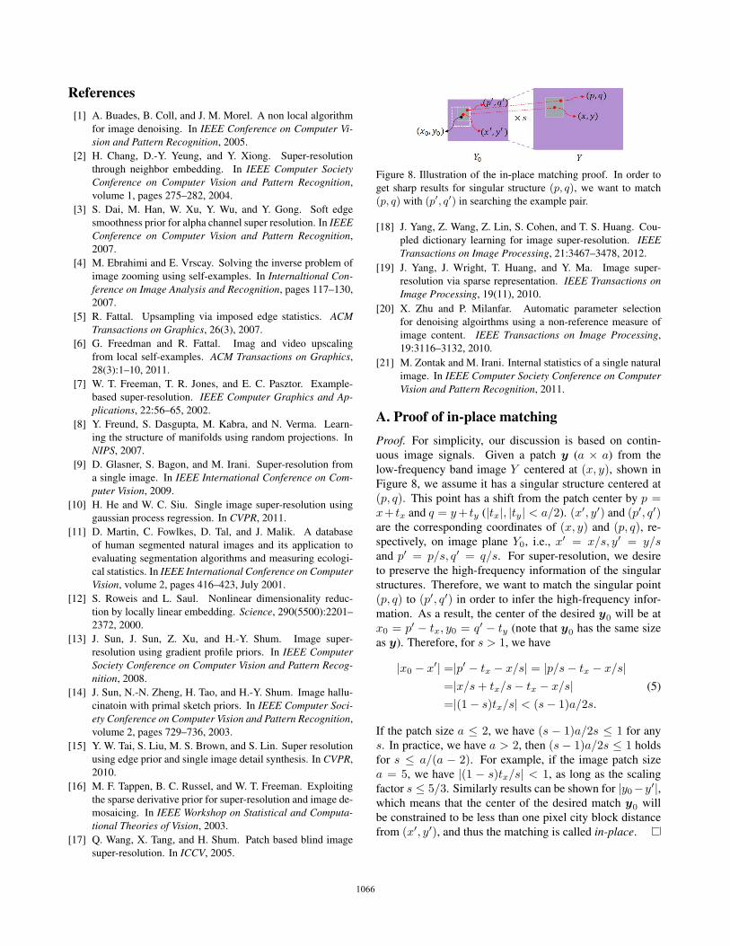
Figure 8. Illustration of the in-place matching proof. In order to
get sharp results for singular structure (p, q), we want to match
(p, q) with (p′, q′) in searching the example pair.
[18] J. Yang, Z. Wang, Z. Lin, S. Cohen, and T. S. Huang. Cou-
pled dictionary learning for image super-resolution. IEEETransactions on Image Processing, 21:3467–3478, 2012.
[19] J. Yang, J. Wright, T. Huang, and Y. Ma. Image super-
resolution via sparse representation. IEEE Transactions onImage Processing, 19(11), 2010.
[20] X. Zhu and P. Milanfar. Automatic parameter selection
for denoising algoirthms using a non-reference measure of
image content. IEEE Transactions on Image Processing,
19:3116–3132, 2010.
[21] M. Zontak and M. Irani. Internal statistics of a single natural
image. In IEEE Computer Society Conference on ComputerVision and Pattern Recognition, 2011.
A. Proof of in-place matchingProof. For simplicity, our discussion is based on contin-
uous image signals. Given a patch y (a × a) from the
low-frequency band image Y centered at (x, y), shown in
Figure 8, we assume it has a singular structure centered at
(p, q). This point has a shift from the patch center by p =x+ tx and q = y+ ty (|tx|, |ty| < a/2). (x′, y′) and (p′, q′)are the corresponding coordinates of (x, y) and (p, q), re-
spectively, on image plane Y0, i.e., x′ = x/s, y′ = y/sand p′ = p/s, q′ = q/s. For super-resolution, we desire
to preserve the high-frequency information of the singular
structures. Therefore, we want to match the singular point
(p, q) to (p′, q′) in order to infer the high-frequency infor-
mation. As a result, the center of the desired y0 will be at
x0 = p′ − tx, y0 = q′ − ty (note that y0 has the same size
as y). Therefore, for s > 1, we have
|x0 − x′| =|p′ − tx − x/s| = |p/s− tx − x/s|=|x/s+ tx/s− tx − x/s|=|(1− s)tx/s| < (s− 1)a/2s.
(5)
If the patch size a ≤ 2, we have (s − 1)a/2s ≤ 1 for any
s. In practice, we have a > 2, then (s − 1)a/2s ≤ 1 holds
for s ≤ a/(a − 2). For example, if the image patch size
a = 5, we have |(1 − s)tx/s| < 1, as long as the scaling
factor s ≤ 5/3. Similarly results can be shown for |y0−y′|,which means that the center of the desired match y0 will
be constrained to be less than one pixel city block distance
from (x′, y′), and thus the matching is called in-place.
10641064106410661066