Fast Fourier Transforms and

Signal Processing

Jake Blanchard

University of Wisconsin - Madison

Spring 2008

Introduction

I’m going to assume here that you know what an FFT is and what you might use it for.

So my intent is to show you how to implement FFTs in Matlab

In practice, it is trivial to calculate an FFT in Matlab, but takes a bit of practice to use it appropriately

This is the same in every tool I’ve ever used

FFTs of Functions

We can sample a function and then take

the FFT to see the function in the

frequency domain

Of course, we must sample often enough

to avoid losing content

The script on the following page samples

a sine wave

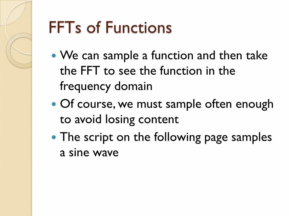
Sampling a sine wave

fo = 4; %frequency of the sine wave

Fs = 100; %sampling rate

Ts = 1/Fs; %sampling time interval

t = 0:Ts:1-Ts;

n = length(t); %number of samples

y = 2*sin(2*pi*fo*t);

plot(t,y)

YfreqDomain = fft(y);

stem(abs(YfreqDomain));

axis([0,100,0,120])

www.blinkdagger.com

Output

0 10 20 30 40 50 60 70 80 90 1000

20

40

60

80

100

120

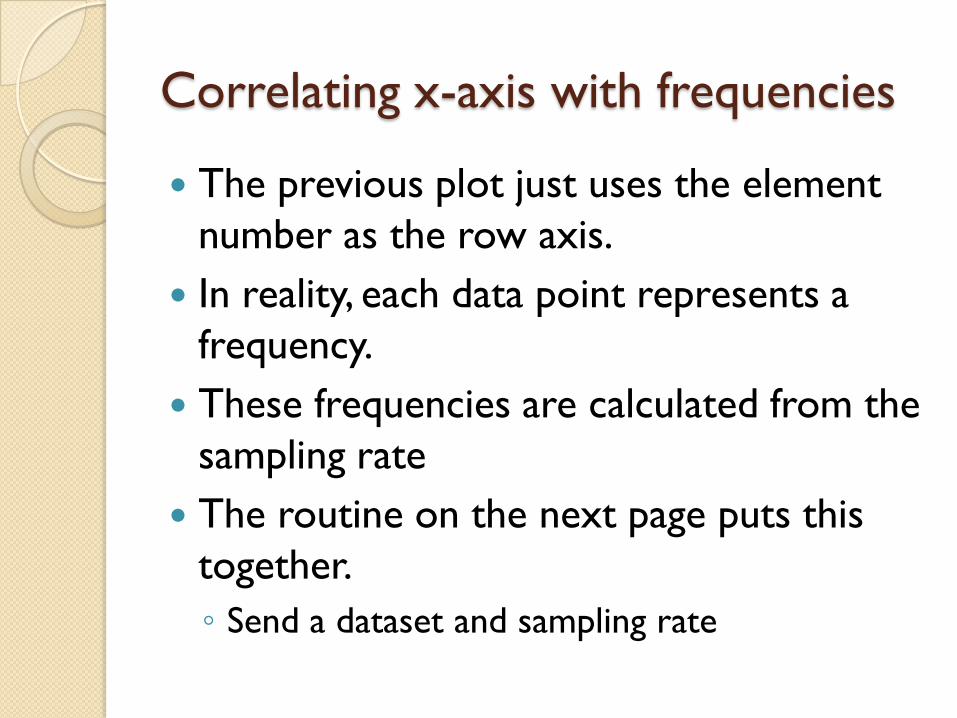
Correlating x-axis with frequencies

The previous plot just uses the element

number as the row axis.

In reality, each data point represents a

frequency.

These frequencies are calculated from the

sampling rate

The routine on the next page puts this

together.

◦ Send a dataset and sampling rate

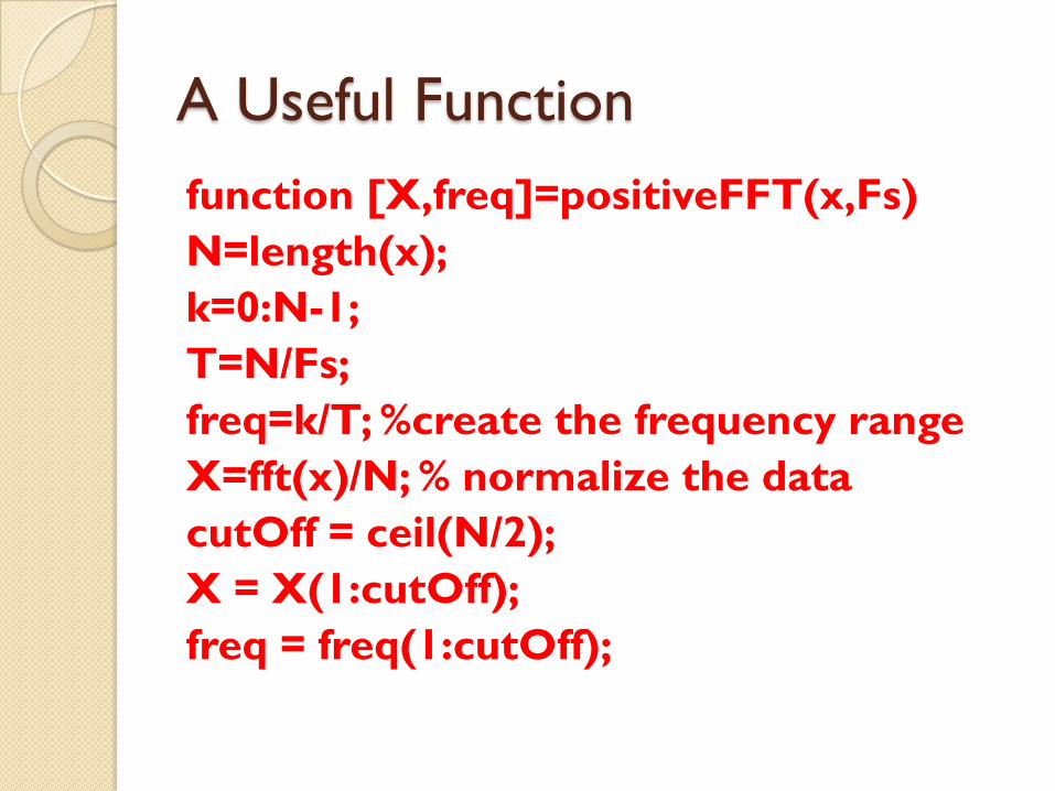
A Useful Function

function [X,freq]=positiveFFT(x,Fs)

N=length(x);

k=0:N-1;

T=N/Fs;

freq=k/T; %create the frequency range

X=fft(x)/N; % normalize the data

cutOff = ceil(N/2);

X = X(1:cutOff);

freq = freq(1:cutOff);

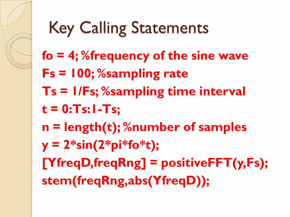
Key Calling Statements

fo = 4; %frequency of the sine wave

Fs = 100; %sampling rate

Ts = 1/Fs; %sampling time interval

t = 0:Ts:1-Ts;

n = length(t); %number of samples

y = 2*sin(2*pi*fo*t);

[YfreqD,freqRng] = positiveFFT(y,Fs);

stem(freqRng,abs(YfreqD));

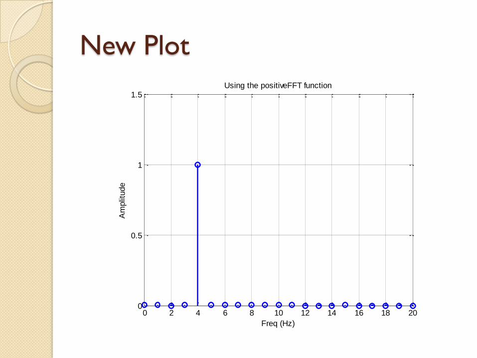
New Plot

0 2 4 6 8 10 12 14 16 18 200

0.5

1

1.5

Freq (Hz)

Am

plit

ude

Using the positiveFFT function

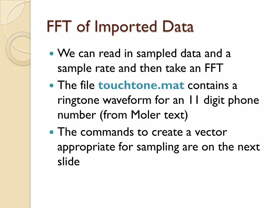
FFT of Imported Data

We can read in sampled data and a

sample rate and then take an FFT

The file touchtone.mat contains a

ringtone waveform for an 11 digit phone

number (from Moler text)

The commands to create a vector

appropriate for sampling are on the next

slide

Script for first number dialed

load touchtone

Fs=y.fs

n = length(y.sig); % number of samples

t = (0:n-1)/y.fs; % Time for entire signal

y = double(y.sig)/128;

t=t(1:8000) % take first 8,000 samples

y=y(1:8000)

plot(t,y)

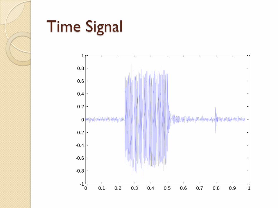
Time Signal

0 0.1 0.2 0.3 0.4 0.5 0.6 0.7 0.8 0.9 1-1

-0.8

-0.6

-0.4

-0.2

0

0.2

0.4

0.6

0.8

1

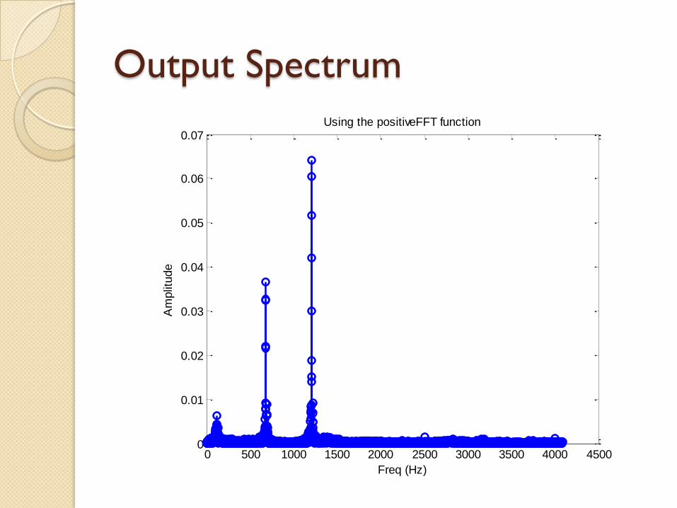
Output Spectrum

0 500 1000 1500 2000 2500 3000 3500 4000 45000

0.01

0.02

0.03

0.04

0.05

0.06

0.07

Freq (Hz)

Am

plit

ude

Using the positiveFFT function

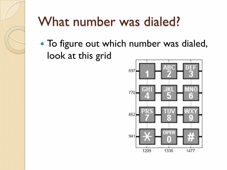
What number was dialed?

To figure out which number was dialed,

look at this grid

What is second number?

Take the next set of data and figure out

which number was dialed.

Try points from 8,000 to 15,000

0 1 2 3 4 5 6 7 8 9 10-1

-0.8

-0.6

-0.4

-0.2

0

0.2

0.4

0.6

0.8

1

Zero Padding (blinkdagger.com)

FFTs work with vectors containing a

number of elements which is an even

power of 2

If you have data which is not a power of 2,

you can fill with 0’s

This will get you faster performance and

better resolution

Example

Beats: y=sin(2f1t)+sin(2f2t)

Let f1=4Hz and f2=4.5Hz

Sample at 100 Hz

Take FFT with and without padding

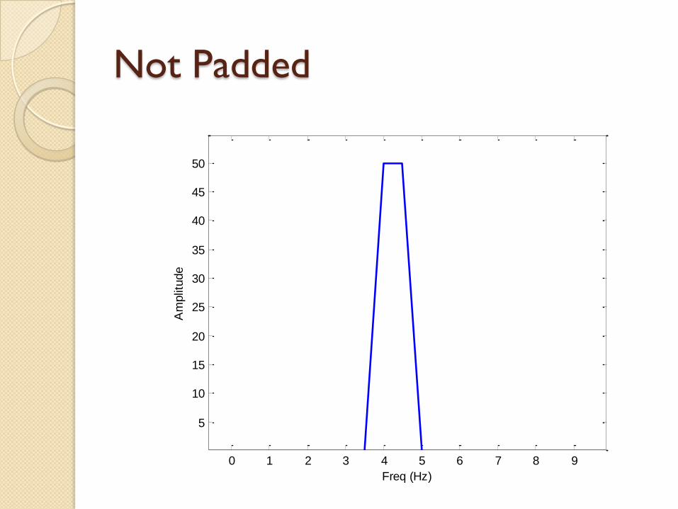
Not Padded

0 1 2 3 4 5 6 7 8 9

5

10

15

20

25

30

35

40

45

50

Freq (Hz)

Am

plit

ude

Zero-Padded

1 2 3 4 5 6 7 8 9 10

5

10

15

20

25

30

35

40

45

50

55

FFT of Sample Signal: Zero Padding up to N = 1024

Freq (Hz)

Magnitude

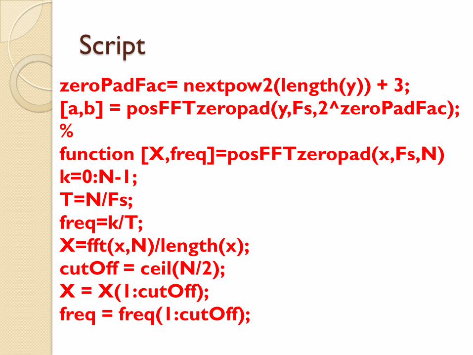
Script

zeroPadFac= nextpow2(length(y)) + 3;

[a,b] = posFFTzeropad(y,Fs,2^zeroPadFac);

%

function [X,freq]=posFFTzeropad(x,Fs,N)

k=0:N-1;

T=N/Fs;

freq=k/T;

X=fft(x,N)/length(x);

cutOff = ceil(N/2);

X = X(1:cutOff);

freq = freq(1:cutOff);

Convolution

Once we can do FFTs, we can do

convolution

Matlab has several built-in

functions for this

To convolve 2 vectors, it is just:

w = conv(u,v)

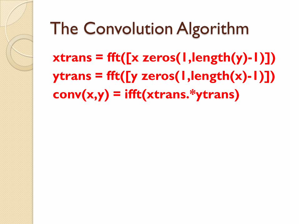
The Convolution Algorithm

xtrans = fft([x zeros(1,length(y)-1)])

ytrans = fft([y zeros(1,length(x)-1)])

conv(x,y) = ifft(xtrans.*ytrans)

2-D Convolution

A = rand(3);

B = rand(4);

C = conv2(A,B)

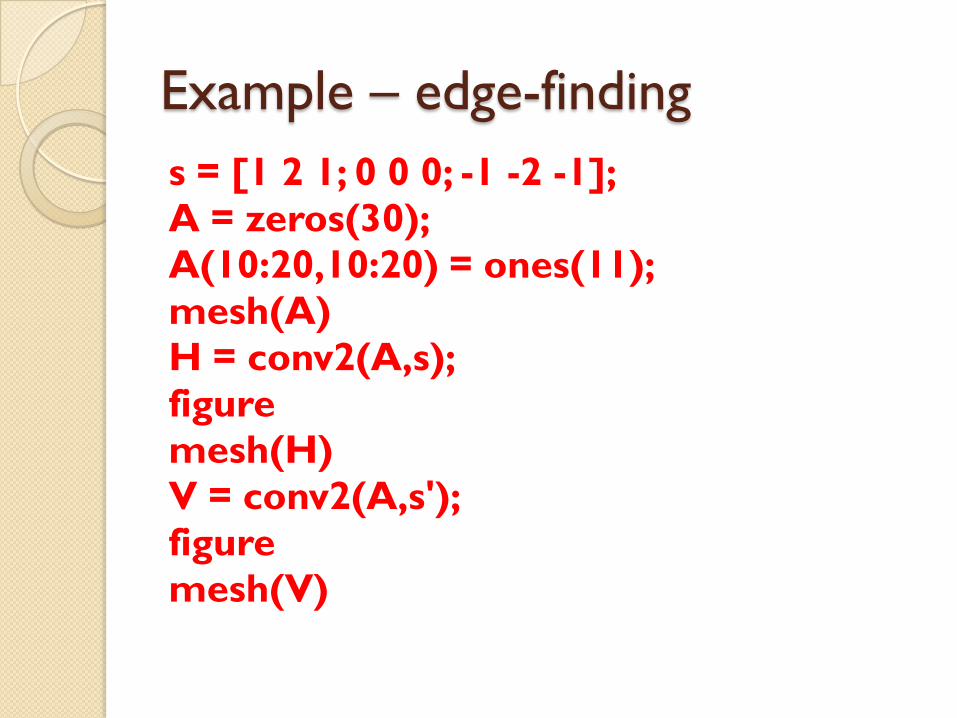
Example – edge-finding

s = [1 2 1; 0 0 0; -1 -2 -1];

A = zeros(30);

A(10:20,10:20) = ones(11);

mesh(A)

H = conv2(A,s);

figure

mesh(H)

V = conv2(A,s');

figure

mesh(V)

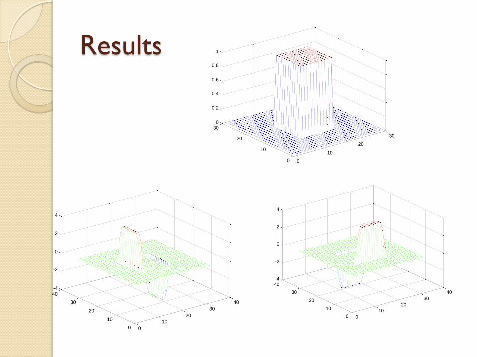
Results

0

10

20

30

0

10

20

300

0.2

0.4

0.6

0.8

1

0

10

20

30

40

0

10

20

30

40-4

-2

0

2

4

0

10

20

30

40

0

10

20

30

40-4

-2

0

2

4

Digital Filters

Matlab has several filters built in

One is the filtfilt command

What is filtfilt?

This is a zero-phase, forward and reverse

digital filter

y=filtfilt(b, a, x)

b and a define filter; x is the data to be

filtered

The length of x must be at least 3 times

the order of the filter (max of length(a)

or length(b) minus 1)

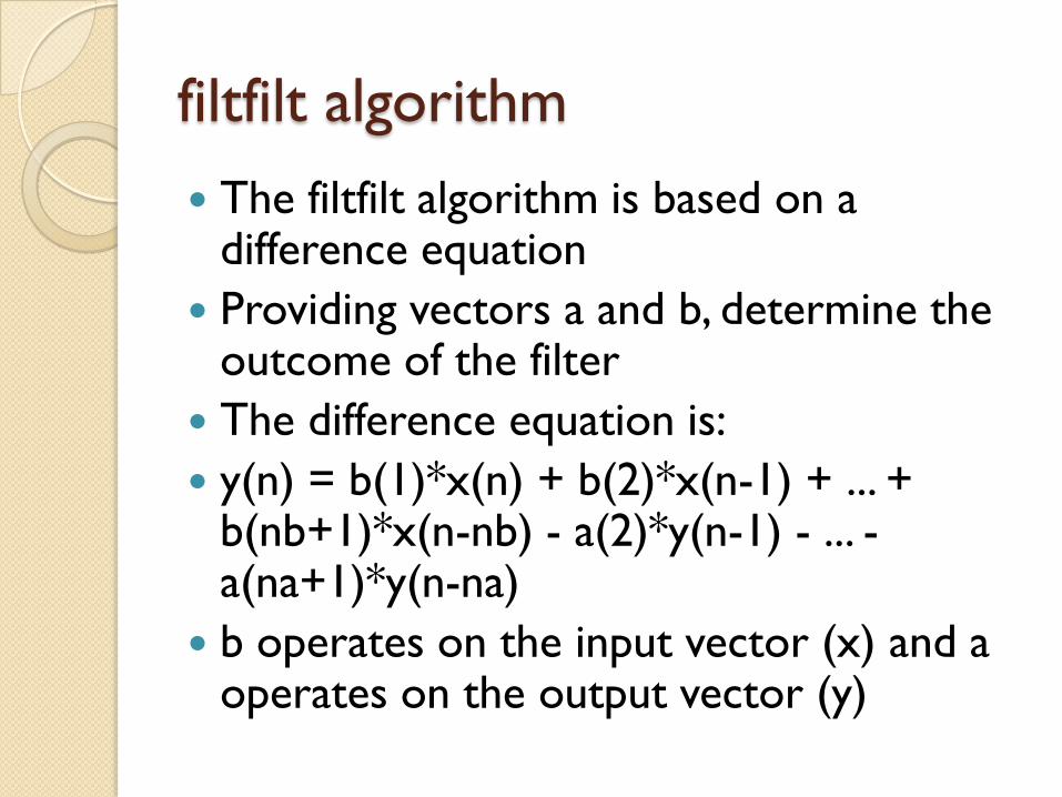
filtfilt algorithm

The filtfilt algorithm is based on a difference equation

Providing vectors a and b, determine the outcome of the filter

The difference equation is:

y(n) = b(1)*x(n) + b(2)*x(n-1) + ... + b(nb+1)*x(n-nb) - a(2)*y(n-1) - ... -a(na+1)*y(n-na)

b operates on the input vector (x) and a operates on the output vector (y)

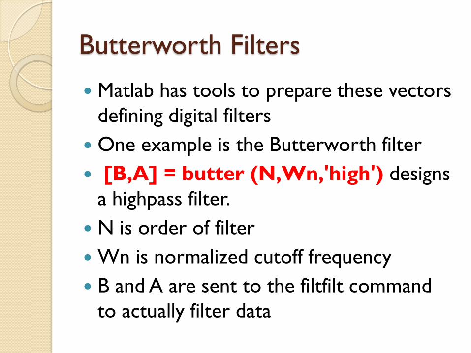
Butterworth Filters

Matlab has tools to prepare these vectors

defining digital filters

One example is the Butterworth filter

[B,A] = butter (N,Wn,'high') designs

a highpass filter.

N is order of filter

Wn is normalized cutoff frequency

B and A are sent to the filtfilt command

to actually filter data

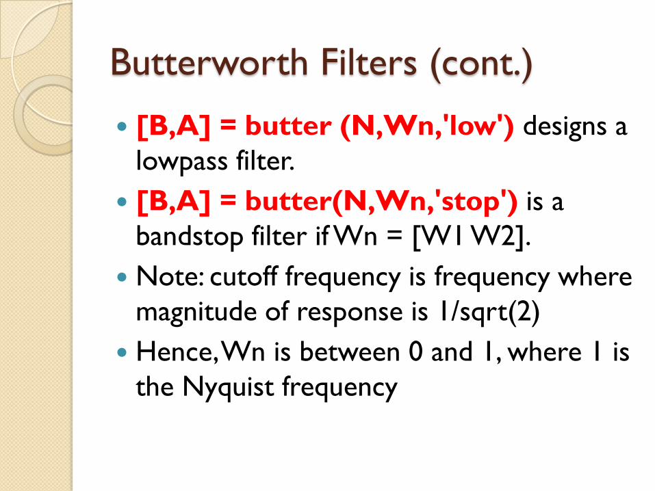
Butterworth Filters (cont.)

[B,A] = butter (N,Wn,'low') designs a

lowpass filter.

[B,A] = butter(N,Wn,'stop') is a

bandstop filter if Wn = [W1 W2].

Note: cutoff frequency is frequency where

magnitude of response is 1/sqrt(2)

Hence, Wn is between 0 and 1, where 1 is

the Nyquist frequency

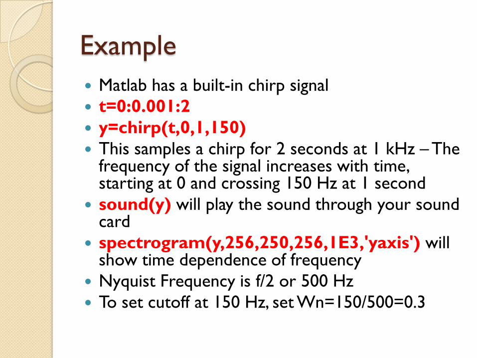
Example

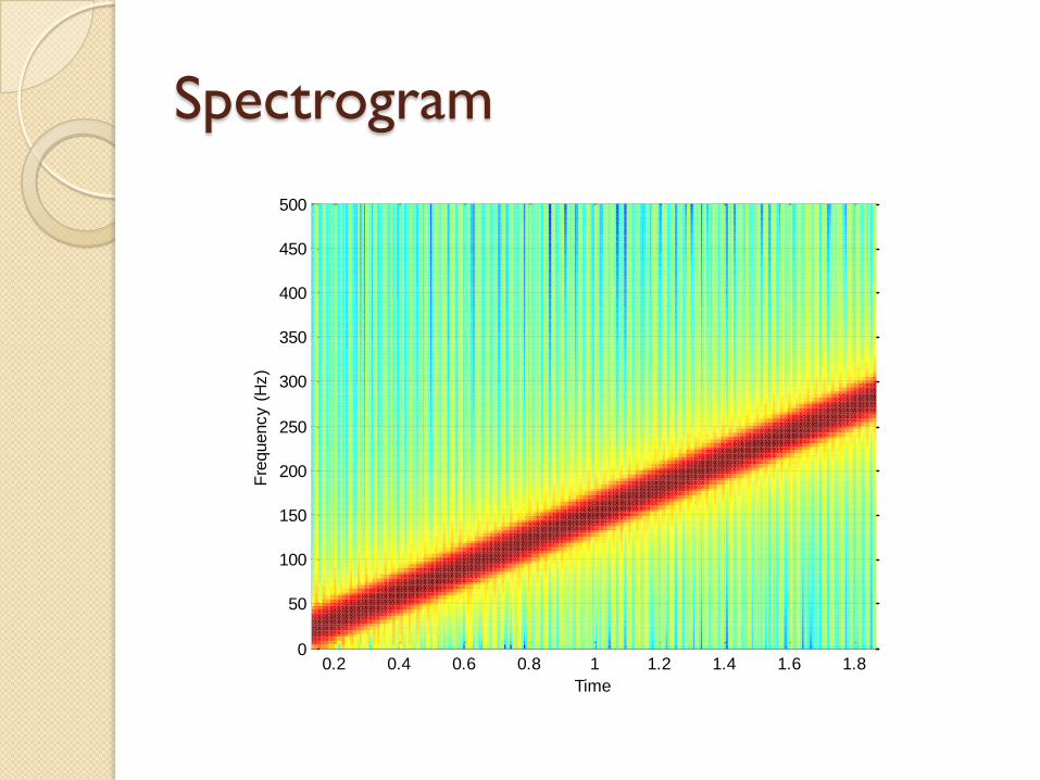
Matlab has a built-in chirp signal

t=0:0.001:2

y=chirp(t,0,1,150)

This samples a chirp for 2 seconds at 1 kHz – The frequency of the signal increases with time, starting at 0 and crossing 150 Hz at 1 second

sound(y) will play the sound through your sound card

spectrogram(y,256,250,256,1E3,'yaxis') will show time dependence of frequency

Nyquist Frequency is f/2 or 500 Hz

To set cutoff at 150 Hz, set Wn=150/500=0.3

Spectrogram

0.2 0.4 0.6 0.8 1 1.2 1.4 1.6 1.80

50

100

150

200

250

300

350

400

450

500

Time

Fre

quency (

Hz)

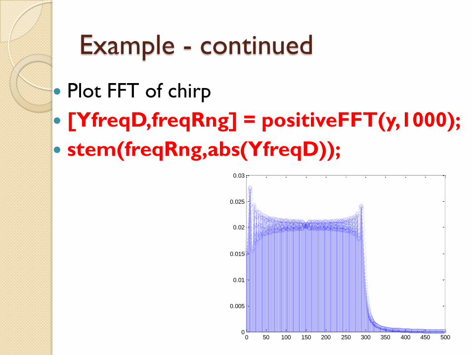
Example - continued

Plot FFT of chirp

[YfreqD,freqRng] = positiveFFT(y,1000);

stem(freqRng,abs(YfreqD));

0 50 100 150 200 250 300 350 400 450 5000

0.005

0.01

0.015

0.02

0.025

0.03

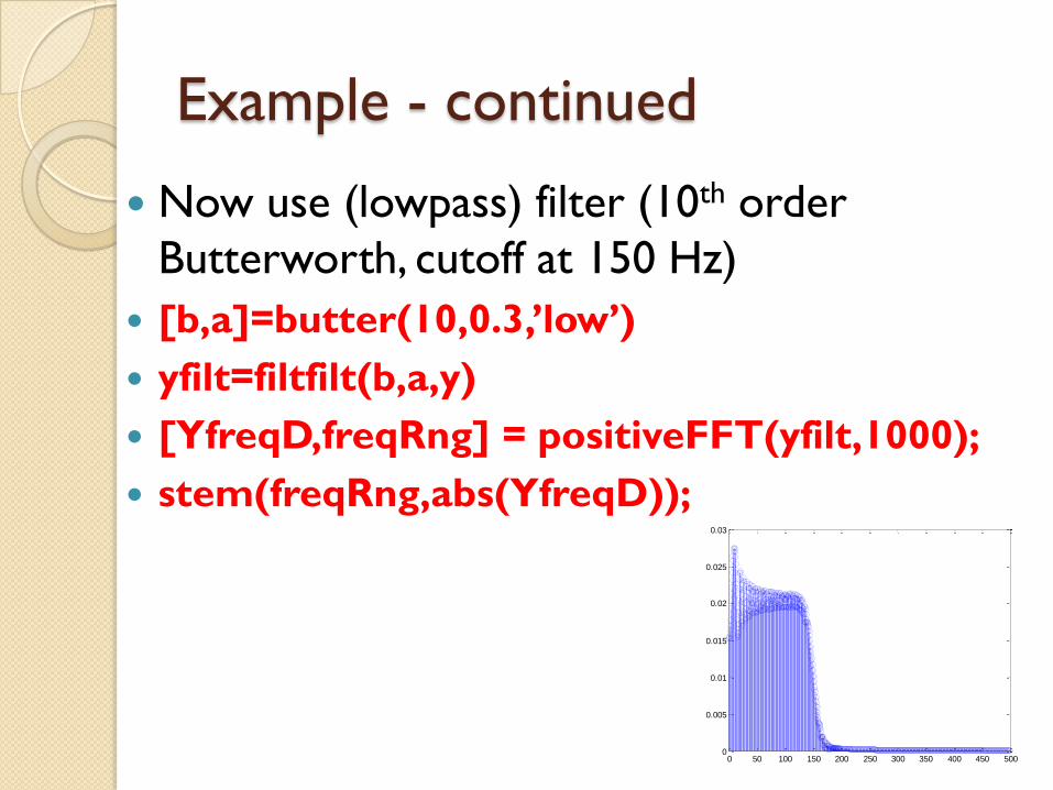
Example - continued

Now use (lowpass) filter (10th order

Butterworth, cutoff at 150 Hz)

[b,a]=butter(10,0.3,’low’)

yfilt=filtfilt(b,a,y)

[YfreqD,freqRng] = positiveFFT(yfilt,1000);

stem(freqRng,abs(YfreqD));

0 50 100 150 200 250 300 350 400 450 5000

0.005

0.01

0.015

0.02

0.025

0.03

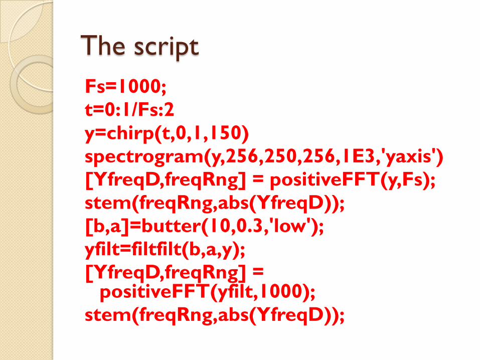
The script

Fs=1000;

t=0:1/Fs:2

y=chirp(t,0,1,150)

spectrogram(y,256,250,256,1E3,'yaxis')

[YfreqD,freqRng] = positiveFFT(y,Fs);

stem(freqRng,abs(YfreqD));

[b,a]=butter(10,0.3,'low');

yfilt=filtfilt(b,a,y);

[YfreqD,freqRng] = positiveFFT(yfilt,1000);

stem(freqRng,abs(YfreqD));

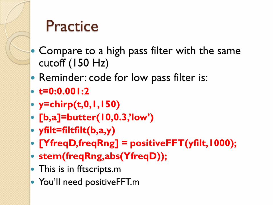
Practice

Compare to a high pass filter with the same cutoff (150 Hz)

Reminder: code for low pass filter is:

t=0:0.001:2

y=chirp(t,0,1,150)

[b,a]=butter(10,0.3,’low’)

yfilt=filtfilt(b,a,y)

[YfreqD,freqRng] = positiveFFT(yfilt,1000);

stem(freqRng,abs(YfreqD));

This is in fftscripts.m

You’ll need positiveFFT.m

Filter Response

To see a filter response, use the freqz or

fvtool from the Signal Processing Toolkit

From previous example:

freqz(b,a,128,Fs) or fvtool(b,a)

This will readily show you impulse

response, step response, pole/zero plots,

etc.

Do you have the SP Toolbox?

Type ver to check

Type help to locate help specific to Signal

Processing Toolbox

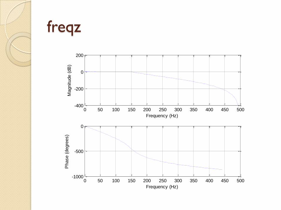
freqz

0 50 100 150 200 250 300 350 400 450 500-1000

-500

0

Frequency (Hz)

Phase (

degre

es)

0 50 100 150 200 250 300 350 400 450 500-400

-200

0

200

Frequency (Hz)

Magnitude (

dB

)

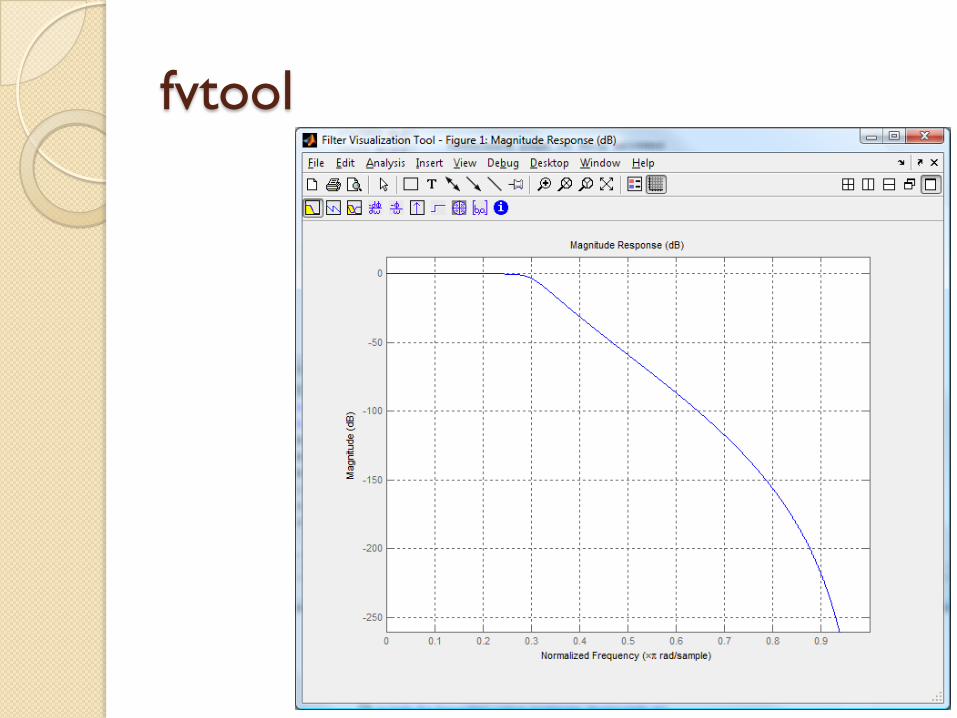
fvtool

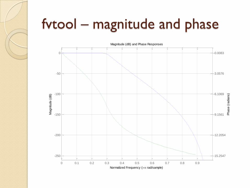
fvtool – magnitude and phase

0 0.1 0.2 0.3 0.4 0.5 0.6 0.7 0.8 0.9

-250

-200

-150

-100

-50

0

Normalized Frequency ( rad/sample)

Magnitu

de (

dB

)

Magnitude (dB) and Phase Responses

-15.2547

-12.2054

-9.1561

-6.1069

-3.0576

-0.0083

Phase (

radia

ns)

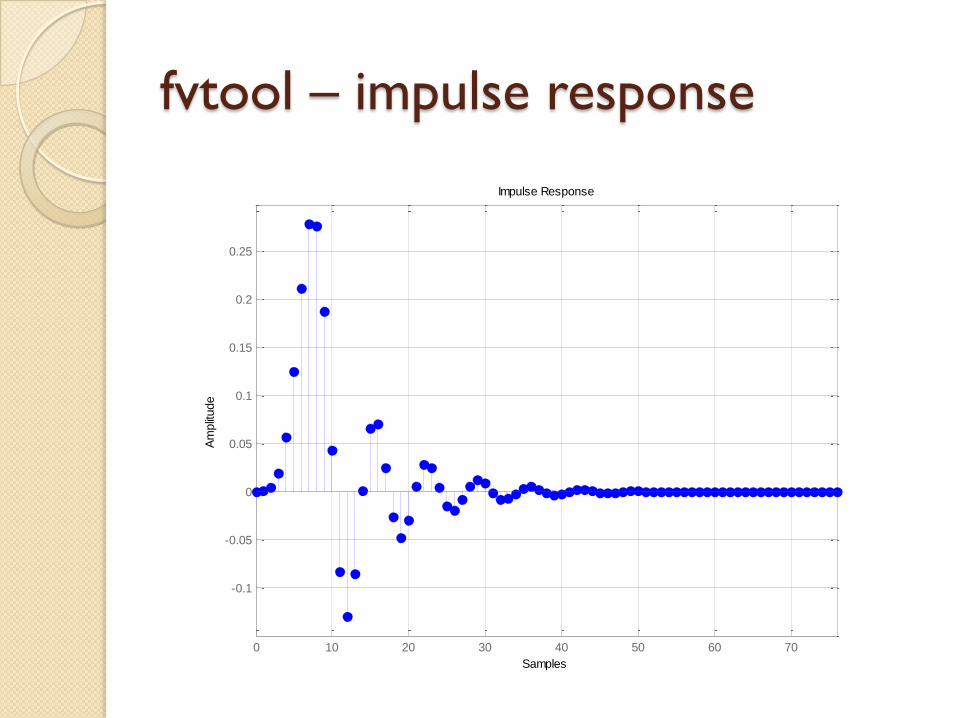
fvtool – impulse response

0 10 20 30 40 50 60 70

-0.1

-0.05

0

0.05

0.1

0.15

0.2

0.25

Samples

Am

plit

ude

Impulse Response

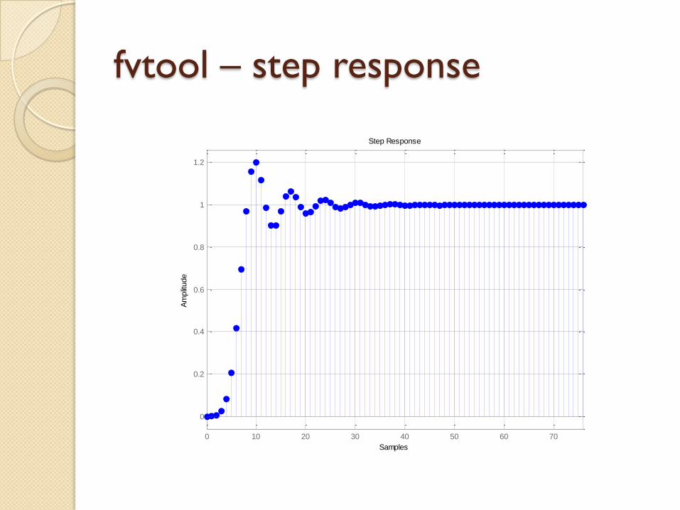
fvtool – step response

0 10 20 30 40 50 60 70

0

0.2

0.4

0.6

0.8

1

1.2

Samples

Am

plit

ude

Step Response

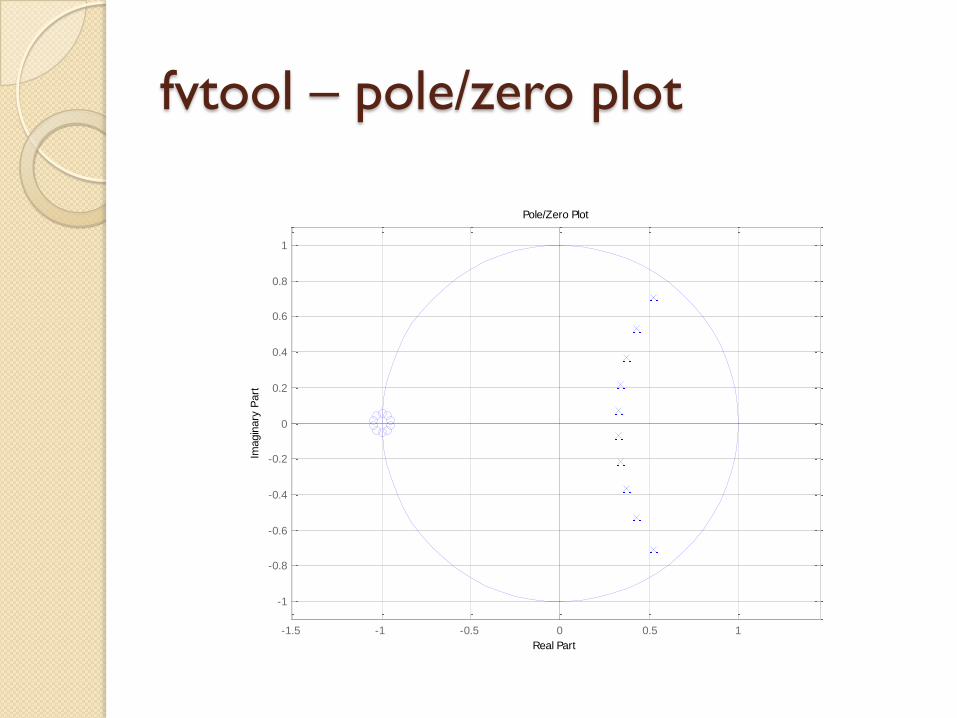
fvtool – pole/zero plot

-1.5 -1 -0.5 0 0.5 1

-1

-0.8

-0.6

-0.4

-0.2

0

0.2

0.4

0.6

0.8

1

Real Part

Imagin

ary

Part

Pole/Zero Plot

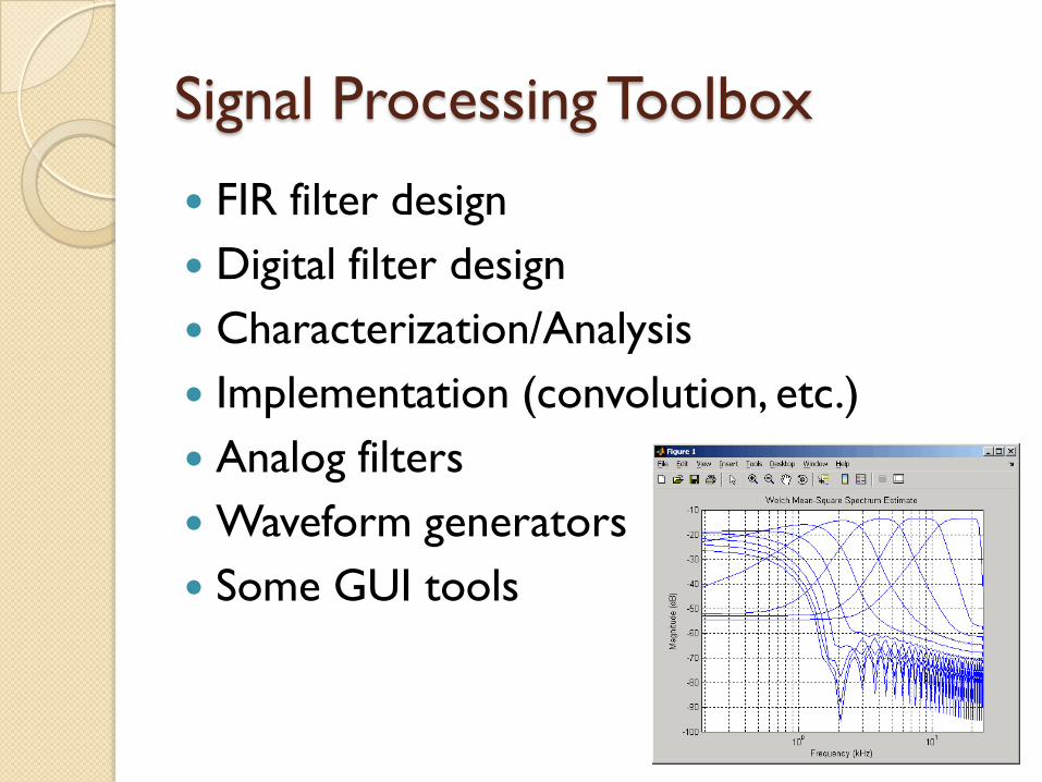
Signal Processing Toolbox

FIR filter design

Digital filter design

Characterization/Analysis

Implementation (convolution, etc.)

Analog filters

Waveform generators

Some GUI tools

Fundamentals

Represent signals as vectors

Step is all 1s

Impulse is a 1 followed by all 0s

Several GUI tools are available:

◦ sptool

◦ fvtool

◦ fdatool

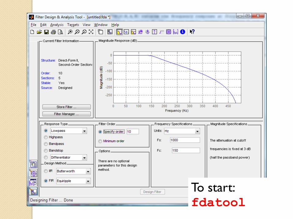
To start:fdatool

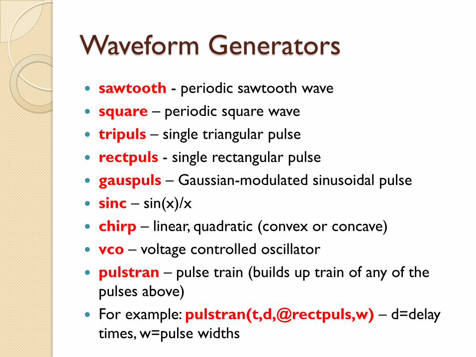
Waveform Generators

sawtooth - periodic sawtooth wave

square – periodic square wave

tripuls – single triangular pulse

rectpuls - single rectangular pulse

gauspuls – Gaussian-modulated sinusoidal pulse

sinc – sin(x)/x

chirp – linear, quadratic (convex or concave)

vco – voltage controlled oscillator

pulstran – pulse train (builds up train of any of the

pulses above)

For example: pulstran(t,d,@rectpuls,w) – d=delay

times, w=pulse widths

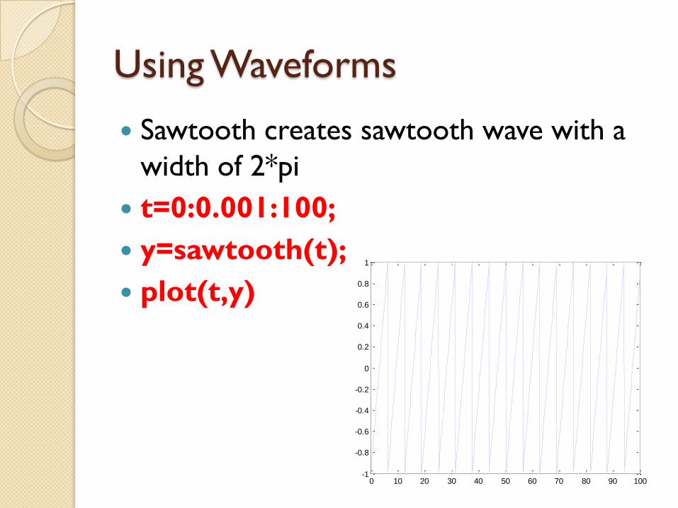
Using Waveforms

Sawtooth creates sawtooth wave with a

width of 2*pi

t=0:0.001:100;

y=sawtooth(t);

plot(t,y)

0 10 20 30 40 50 60 70 80 90 100-1

-0.8

-0.6

-0.4

-0.2

0

0.2

0.4

0.6

0.8

1

Spectral Analysis

psd – power spectral density

msspectrum – mean square

pseudospectrum

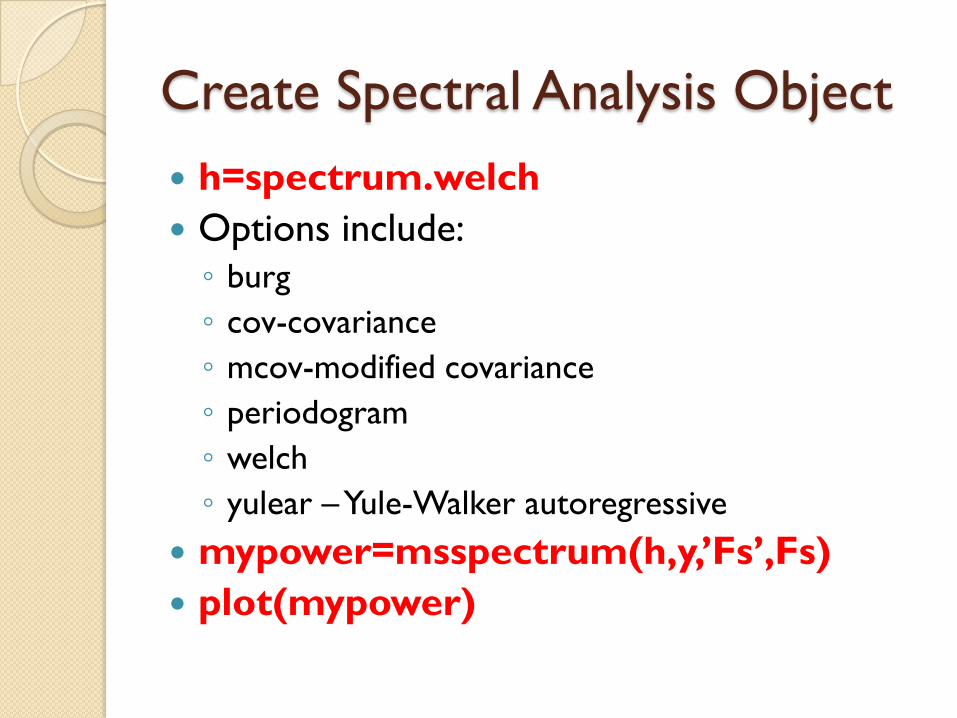
Create Spectral Analysis Object

h=spectrum.welch

Options include:

◦ burg

◦ cov-covariance

◦ mcov-modified covariance

◦ periodogram

◦ welch

◦ yulear –Yule-Walker autoregressive

mypower=msspectrum(h,y,’Fs’,Fs)

plot(mypower)

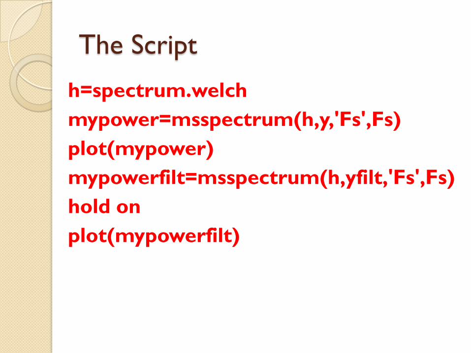
The Script

h=spectrum.welch

mypower=msspectrum(h,y,'Fs',Fs)

plot(mypower)

mypowerfilt=msspectrum(h,yfilt,'Fs',Fs)

hold on

plot(mypowerfilt)

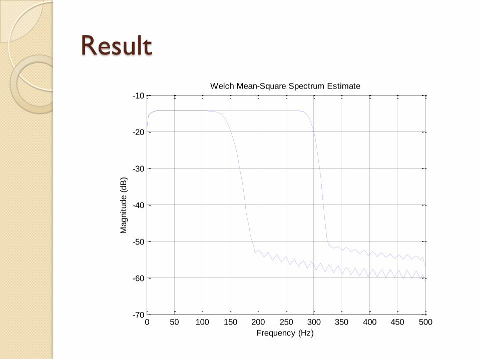
Result

0 50 100 150 200 250 300 350 400 450 500-70

-60

-50

-40

-30

-20

-10

Frequency (Hz)

Magnitude (

dB

)

Welch Mean-Square Spectrum Estimate

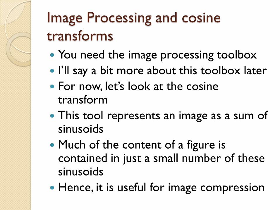
Image Processing and cosine

transforms

You need the image processing toolbox

I’ll say a bit more about this toolbox later

For now, let’s look at the cosine transform

This tool represents an image as a sum of sinusoids

Much of the content of a figure is contained in just a small number of these sinusoids

Hence, it is useful for image compression

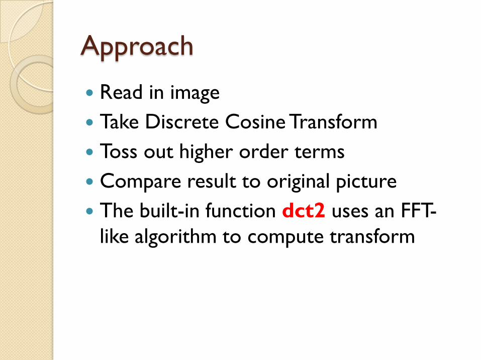
Approach

Read in image

Take Discrete Cosine Transform

Toss out higher order terms

Compare result to original picture

The built-in function dct2 uses an FFT-

like algorithm to compute transform

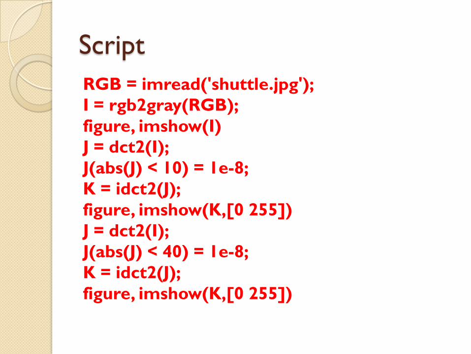
Script

RGB = imread('shuttle.jpg');

I = rgb2gray(RGB);

figure, imshow(I)

J = dct2(I);

J(abs(J) < 10) = 1e-8;

K = idct2(J);

figure, imshow(K,[0 255])

J = dct2(I);

J(abs(J) < 40) = 1e-8;

K = idct2(J);

figure, imshow(K,[0 255])

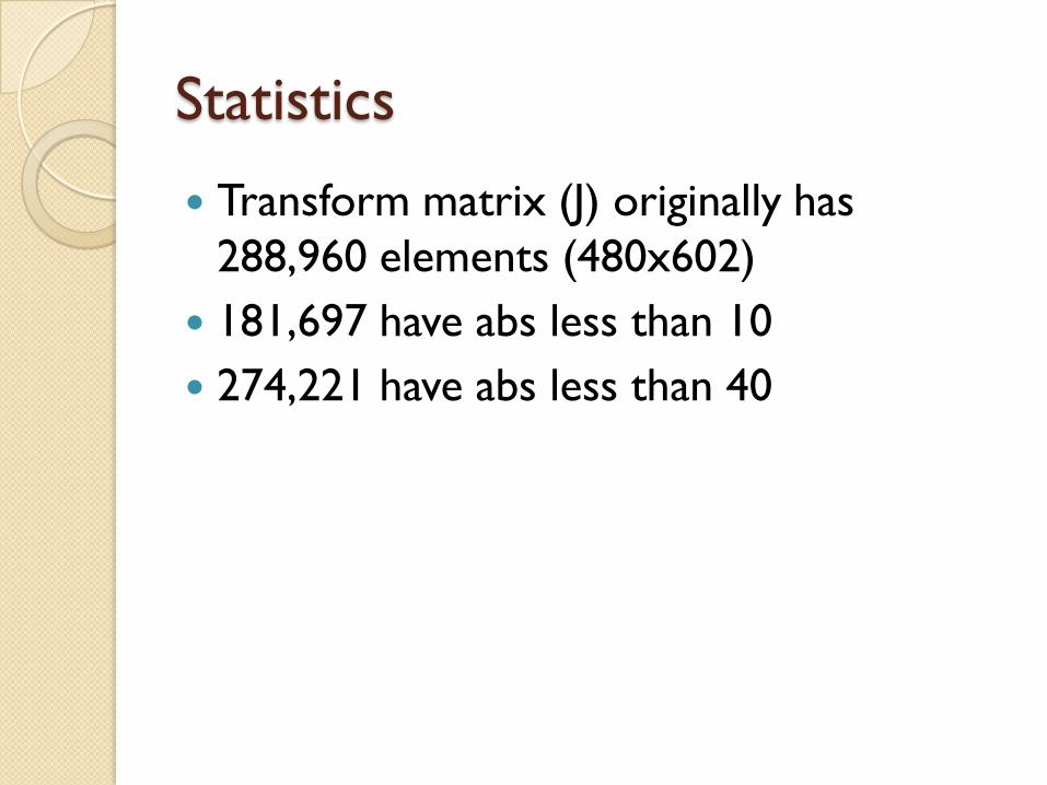
Statistics

Transform matrix (J) originally has

288,960 elements (480x602)

181,697 have abs less than 10

274,221 have abs less than 40

First Compression (abs(J)<10)

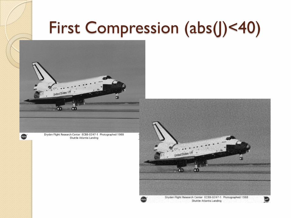
First Compression (abs(J)<40)

Questions?