Embed Size (px)
Citation preview

________________
Received December 11, 2014
280
FAST FINITE ELEMENT SOLVER FOR INCOMPRESSIBLE NAVIER-
STOKES EQUATION BY PARALLEL GRAM-SCHMIDT PROCESS BASED
GMRES AND HSS
DI ZHAO
Supercomputing Center, Chinese Academy of Sciences, Beijing, 100190
Copyright © 2015 Di Zhao. This is an open access article distributed under the Creative Commons Attribution License, which permits
unrestricted use, distribution, and reproduction in any medium, provided the original work is properly cited.
Abstract. After finite element discretization of incompressible Navier-Stokes equation, a sparse linear system is
obtained in every iteration, and GMRES provides an efficient approach to solve this system. However, if the size of
the original PDE model is large, the solution speed of the incompressible Navier-Stokes equation is still slow. Since
the linear system from the incompressible Navier-Stokes equation is saddle point problem, we find that large portion
of computational efforts for solving the linear system is occupied by the vector projection in GMRES. In this paper,
by our parallel Gram-Schmidt process based GMRES and newly developed preconditioner Hermitian/Skew-
Hermitian Separation (HSS), we develop a fast solver HSS-pGMRES for the saddle point problem from
incompressible Navier-Stokes Equation. Theoretical analysis shows that, HSS-pGMRES decreases the
computational complexity of finite element solver for incompressible Navier-Stokes equation from O(m2n) to O(mn),
where m is the grid size. Computational experiments show that, the fast solver HSS-pGMRES significantly increases
the solution speed for the saddle point problem of incompressible Navier-Stokes equation than the conventional
solvers.
Keywords: fast solver; vector projection; parallel GMRES; Hermitian/Skew-Hermitian Separation; finite element
method; incompressible Navier-Stokes equation.
2010 AMS Subject Classification: 76M10.
1. INTRODUCTION
The incompressible Navier-Stokes equation is a mass conservation and momentum conservation
based mathematical equation. Besides the fluid density ρ is fixed, the incompressible Navier-
Stokes decides two fundamental properties of a flow: the velocity u and the pressure p in a flow
Available online at http://scik.org
J. Math. Comput. Sci. 5 (2015), No. 3, 280-296
ISSN: 1927-5307

FAST FINITE ELEMENT SOLVER 281
field along with the time t, and the boundary condition of the flow field and the initial condition
for the time t provide the uniqueness of the two variables.
Incompressible Navier-Stokes equation is usually solved by numerical methods such as finite
difference method or finite element method: Anderson studied the numerical solution of Navier-
Stokes equation by finite difference method in [1], and Elman et al. studied finite element
solution of incompressible Navier-Stokes equation in [2].
Numerically solving incompressible Navier-Stokes equation is slow when the grid size is large,
acceleration methods for Navier-Stokes equation are developed to accelerate the solution speed,
and these approaches include high-order discretization [3-5], preconditioning, parallel computing
[6-13], GPU computing, etc.
The linear system from the discretization of incompressible Navier-Stokes equation is often
solved by sparse solvers such as GMRES, and GMRES stands for Generalized Minimal Residual
Method [14]. Performance improvement of GMRES is studied in [15, 16], and parallel GMRES
is one of possible approaches to accelerate the solution speed of incompressible Navier-Stokes
equation.
Preconditioner is another approach to accelerate the solution speed of incompressible Navier-
Stokes equation. Elman et al. developed kinds of preconditioners in [17-21], and Benzi et al.
developed preconditioners for the system [22, 23].
If the size of the original PDE model is large, the solution speed of the incompressible Navier-
Stokes equation is still slow. Since the linear system from the incompressible Navier-Stokes
equation is the saddle point problem, we find that large portion of computational efforts of
solving the linear system is invested on the vector projection in GMRES. In this paper, by our
parallel Gram-Schmidt process based GMRES and newly developed preconditioner
Hermitian/Skew-Hermitian Separation (HSS) for the saddle point problem, we develop a fast
solver HSS-pGMRES for incompressible Navier-Stokes equation.
2. METHODS
In this section, we firstly discuss the preconditioner Hermitian/Skew-Hermitian Separation, then
we develop parallel GMRES, and we develop the fast solver HSS-pGMRES for the saddle point

282 DI ZHAO
problem. Finally, HSS-pGMRES is applied to incompressible Navier-Stokes equation for a fast
solution.
2.1 The Hermitian/Skew-Hermitian Separation
Saddle point matrix is a matrix with the form:
[𝐹 𝐷𝑇
𝐷 −𝐸] [𝑑𝑢𝑑𝑝
] = [𝑅𝑑𝑟𝑑], (1)
where F and E are usually symmetric matrices [24], du and dp are unknown variables, and Rd
and rd are right-hand-side. Saddle point problems appear in high-frequency in scientific and
engineering applications. Golub reviewed solution methods for saddle point problem in [24], and
the solution methods for saddle point problem include Schur complement reduction, null space
methods, coupled direct solvers, stationary iterations, Krylov subspace methods, preconditioner
and multilevel methods [24].
Newly developed matrix splitting based methods such as HSS provide an efficient way to solve
saddle point problems [25-27]. Golub et al. developed HSS in [28], parameter optimization for
HSS is proposed in [29], and preconditioned HSS is studied in [30-35].
To efficiently solve a linear system with the structure of saddle point problem of equation (1)
with the symmetric part H and the skew-symmetric part S, we firstly solve an uncoupled linear
system:
(𝐻 + 𝛼𝐼𝑛) ∙ 𝑑𝑢𝑘+
1
2 = 𝑓𝑢𝑐𝑘 , (2.1)
(𝐸 + 𝛼𝐼𝑚) ∙ 𝑑𝑝𝑘+
1
2 = 𝑔𝑢𝑐𝑘 . (2.2)
where fuck and guc
k are right-hand-side. Then we solve a coupled linear system:
(𝛼𝐼𝑛 + 𝑆) ∙ 𝑑𝑢𝑘+1 + 𝐷𝑇 ∙ 𝑑𝑝𝑘+1 = 𝑓𝑐𝑘, (3.1)
−𝐷 ∙ 𝑑𝑢𝑘+1 + 𝛼𝑝𝑘+1 = 𝑔𝑐𝑘. (3.2)
where fk and gk are right-hand-side. By Schur complement reduction, we obtain:
[𝐷(𝐼𝑛 + 𝛼−1𝑆)−1𝐷𝑇 + 𝛼2𝐼𝑚] ∙ 𝑑𝑝𝑘+1 = 𝐷(𝐼𝑛 + 𝛼−1𝑆)−1𝑓𝑘 + 𝛼𝑔𝑘. (4)
Since the coefficient matrix [D(In + α−1S)−1DT + α2Im] of equations (4) is large and sparse matrix,
GMRES is applied to solve 𝑑𝑝𝑘+1, then we obtain 𝑑𝑢𝑘+1. The details of HSS are described in
Algorithm 1:
Algorithm 1: The Hermitian/Skew-Hermitian Separation

FAST FINITE ELEMENT SOLVER 283
Initialization of HSS
while R < tolHSS
Solve the couple system equations (2)
Solve the uncoupled system equations (3)
end while
Convergence analysis of HSS (Algorithm 1) can be found in [30], and the convergence speed of
HSS (Algorithm 1) is decided by tolHSS. However, the linear systems are unnecessary to be
solved exactly, and the tolerance of the iterative solver for the linear systems can be loosened to
increase the solution speed, which leads to inexact HSS.
2.2 Parallel GMRES
As we discussed, the uncoupled system equations (4) in HSS (Algorithm 1) can be solved by
sparse solvers such as GMRES, and the details of GMRES are described in Algorithm 2:
Algorithm 2: GMRES
Initialization of GMRES
while Rk < tolGMRES
𝑤0𝑘+1 = 𝐴 ∙ 𝑣𝑘
𝑣𝑖+1𝑘+1 = 𝑣𝑖
𝑘+1 − ∑ 𝑃(𝑤𝑖𝑘+1, 𝑣𝑖)
𝑘−1𝑖=1
Calculate yk such that 𝑅𝑘 = 𝑚𝑖𝑛‖𝑅0𝑒1 − 𝐻𝑘𝑦𝑘‖
end while
𝑢𝑘 = 𝑢0 + 𝑉𝑘𝑦𝑘
In GMRES (Algorithm 2), Gram-Schmidt process is chosen to build the orthogonal set u. In
details of Gram-Schmidt process, the vector projection is defined as:
𝑃(𝑢, 𝑣) =⟨𝑢,𝑣⟩
⟨𝑢,𝑢⟩𝑢. (5)
Gram-Schmidt process works as:
𝑢1 = 𝑣1,
𝑢𝑘 = 𝑣𝑘 − ∑ 𝑃(𝑢𝑖, 𝑣𝑖)𝑘−1𝑖=1 . (6)

284 DI ZHAO
In GMRES (Algorithm 2), large portion of computational efforts is spent on building the
orthogonalization basis in Gram-Schmidt process, and statistics from computational experiments
show that the ratio of computational cost of Gram-Schmidt process to GMRES (Algorithm 2) is
about 1/4. To further increase the solution speed of GMRES (Algorithm 2), the process of
building the orthogonalization basis can be parallelized for higher efficiency, and the parallel
strategy for Gram-Schmidt process based GMRES (pGMRES) is illustrated in Figure 1.
Figure 1. Parallel Strategy for Gram-Schmidt Process based GMRES
pGMRES is designed to simultaneously calculate the vector projection P(u, v) of equation (5).
From Figure 1 we can see, every thread is responsible for calculating a the vector projection P(u,
v) of equation (5), and a reduction is followed to calculate the summation in equation (6). The
number of the vector projection P(u, v) of equation (5) increases in the summation of equation (6)
along with pGMRES iterations. However, the number of threads for pGMRES must keep the
same in Figure 1. To settle this conflict, the redundant threads calculate vectors with all zero
elements to keep the load balance of threads.
Algorithm 3: Parallel Gram-Schmidt Process based GMRES
Initialization of GMRES
while Rk < tolGMRES
𝑤0𝑘+1 = 𝐴 ∙ 𝑣𝑘
W1k+1, v1
W2k+1, v2
Wkk+1, vk
WKk+1, vK
vectorProjection 1 at thread 1
vectorProjection 2 at thread 2
vectorProjection k at thread k
vectorProjection K at thread K
P1
P2
Pk
PK
reduction
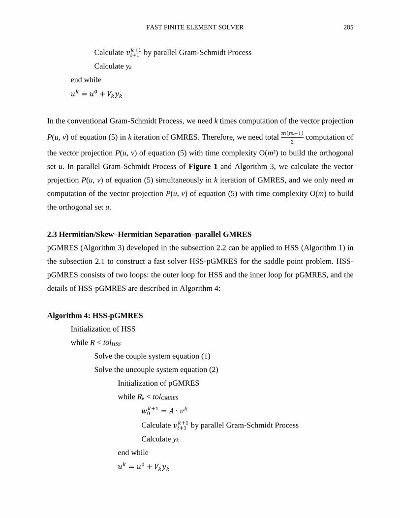
FAST FINITE ELEMENT SOLVER 285
Calculate 𝑣𝑖+1𝑘+1 by parallel Gram-Schmidt Process
Calculate yk
end while
𝑢𝑘 = 𝑢0 + 𝑉𝑘𝑦𝑘
In the conventional Gram-Schmidt Process, we need k times computation of the vector projection
P(u, v) of equation (5) in k iteration of GMRES. Therefore, we need total 𝑚(𝑚+1)
2 computation of
the vector projection P(u, v) of equation (5) with time complexity O(m²) to build the orthogonal
set u. In parallel Gram-Schmidt Process of Figure 1 and Algorithm 3, we calculate the vector
projection P(u, v) of equation (5) simultaneously in k iteration of GMRES, and we only need m
computation of the vector projection P(u, v) of equation (5) with time complexity O(m) to build
the orthogonal set u.
2.3 Hermitian/Skew–Hermitian Separation–parallel GMRES
pGMRES (Algorithm 3) developed in the subsection 2.2 can be applied to HSS (Algorithm 1) in
the subsection 2.1 to construct a fast solver HSS-pGMRES for the saddle point problem. HSS-
pGMRES consists of two loops: the outer loop for HSS and the inner loop for pGMRES, and the
details of HSS-pGMRES are described in Algorithm 4:
Algorithm 4: HSS-pGMRES
Initialization of HSS
while R < tolHSS
Solve the couple system equation (1)
Solve the uncouple system equation (2)
Initialization of pGMRES
while Rk < tolGMRES
𝑤0𝑘+1 = 𝐴 ∙ 𝑣𝑘
Calculate 𝑣𝑖+1𝑘+1 by parallel Gram-Schmidt Process
Calculate yk
end while
𝑢𝑘 = 𝑢0 + 𝑉𝑘𝑦𝑘

286 DI ZHAO
end while
In the conventional GMRES (Algorithm 2), we need k times computation of the vector
projection P(u, v) of equation (5) in k iteration of GMRES and n iteration of HSS (Algorithm 1).
Therefore, we need total 𝑚(𝑚+1)𝑛
2 computation of the vector projection P(u, v) of equation (5)
with time complexity O(m²n) to build all orthogonal sets. In HSS-pGMRES (Algorithm 4), we
calculate the vector projection P(u, v) of equation (5) simultaneously in k iteration of GMRES
and n iteration of HSS (Algorithm 1), and we only need mn computation of the vector projection
P(u, v) of equation (5) with time complexity O(mn) to build the orthogonal set u.
2.4 HSS-pGMRES for Incompressible Navier-Stokes equation
In this subsection, we apply HSS-pGMRES (Algorithm 4) to fast solve the saddle point problem
from incompressible Navier-Stokes equation, which is discretized by finite element method. The
time-independent incompressible Navier-Stokes equation is:
−𝑘∆𝑢 + 𝑢 ∙ ∇𝑢 + ∇𝑝 = 𝑓, (6.1)
∇ ∙ 𝑢 = 0, (6.2)
where k is kinematic viscosity, u is velocity, p is pressure and f is the force term.
Firstly we approximate u by velocity basis function φi and p by pressure basis function ψj, and
we obtain:
𝑘 ∫∇𝜑𝑖 ∙ ∇𝜑𝑗 + ∫(𝑢∗ ∙ ∇𝜑𝑗)𝜑𝑗 + ∫(𝜑𝑗 ∙ ∇𝑢∗)𝜑𝑗 − 𝑘 ∫∇𝜑𝑖 ∙ ∇𝜑𝑗 = 𝑅𝑑,
∫𝜑𝑘 ∙ ∇𝜑𝑗 = 𝑟𝑑,
where Rd and rd is the right-hand-side. Setting
𝐴 = ∫∇𝜑𝑖 ∙ ∇𝜑𝑗,
𝐵 = ∫∇𝜑𝑖 ∙ ∇𝜑𝑗,
𝐶 = ∫∇𝜑𝑖 ∙ ∇𝜑𝑗,
𝐷 = ∫∇𝜑𝑖 ∙ ∇𝜑𝑗,
we obtain the linear system of the saddle point problem of equation (1). A posteriori error
estimate is used for error analysis, and the estimated error is plotted based on grid used in the
specific problem [2].

FAST FINITE ELEMENT SOLVER 287
In the conventional GMRES (Algorithm 2) for incompressible Navier-Stokes equation, we need
k times computation of the vector projection P(u, v) of equation (5) in k iteration of GMRES and
n iteration of HSS (Algorithm 1). Therefore, we need total 𝑚(𝑚+1)𝑛
2 computation of the vector
projection P(u, v) of equation (5) with time complexity O(m²n) to solve incompressible Navier-
Stokes equation. In HSS-pGMRES (Algorithm 4) for incompressible Navier-Stokes equation, we
calculate the vector projection P(u, v) of equation (5) simultaneously in k iteration of GMRES
and n iteration of HSS (Algorithm 1), and we only need mn computation of the vector projection
P(u, v) of equation (5) with time complexity O(mn) for solving incompressible Naiver-Stokes
equation. Meanwhile, m usually means the grid size for discretization of incompressible Navier-
Stokes equation, either by finite element method or finite difference method.
3. COMPUTATIONAL RESULTS
3.1 The Problem
To test the performance of HSS-pGMRES (Algorithm 4) for incompressible Navier-Stokes
equation, we set f = 0 in equation (6.1) in the square −1 ≤ x ≤ 1 and −1 ≤ y ≤ 1. The inflow
boundary is set as the Dirichlet condition x = −1, and the outflow boundary is set as the
Neumann condition:
𝜕𝑢𝑥
𝜕𝑥− 𝑝 = 0,
𝜕𝑢𝑦
𝜕𝑦= 0.
We coded HSS-pGMRES (Algorithm 4), and the discretization of incompressible Navier-Stokes
equation is based on IFISS [36]. The server is Intel Core 2 2.66 GHz CPU and 4G ECC 800MHz
memory (DELL XPS 410). We test the performance of HSS-pGMRES (Algorithm 4), and all
numerical experiments are repeated for three times.
3.2 Performance of HSS-pGMRES
In this experiment, we compare time cost of three different solvers: Gauss Jordan Elimination
(GJE), HSS-GJE and HSS-pGMRES (Algorithm 4) for incompressible Navier-Stokes equation.
The grid in this experiment is 8×8. In HSS-pGMRES (Algorithm 4), we set tolHSS = 10⁻² and

288 DI ZHAO
tolGMRES = 10⁻¹². The time cost of all three solvers is tested for three times, average values and
standard deviations are plotted in Figure 2.
Figure 2. The time cost of the three solvers for incompressible Navier-Stokes equation: GJE,
HSS-GJE and HSS-pGMRES
From Figure 2 we can see, to solve a linear system with the same size, HSS-pGMRES
(Algorithm 4) is the fastest, HSS-GJE is the middle, and GJE is the slowest. To quantitatively
measure the acceleration of every solver, we define the acceleration rate as the following:
𝑟𝑎𝑡𝑒 =𝑡𝑠𝑙𝑜𝑤𝑒𝑠𝑡
𝑡𝑖,
where tslowest is the time cost of the slowest solver GJE, ti is the time cost of a testing solver, and
rate is the calculated acceleration rate. The calculated acceleration rates for the three solvers GJE,
HSS-GJE and HSS-pGMRES (Algorithm 4) are listed in Table 1.
Table 1. Calculated acceleration rate for the three solvers: GJE, HSS-GJE and HSS-pGMRES
GJE HSS-GJE HSS-pGMRES
Acceleration rate 1.00 2.71 12.93
From Table 1 we can see, HSS-pGMRES (Algorithm 4) is about 12.93 times faster than GJE,
and HSS-GJE is about 2.71 times faster than GJE. From Figure 2 and Table 1 we can see, HSS-
GJE
inexactHSS-
GJE
inexactHSS-
pGMRES
0
25
50
75
100
125
150
175
200
225ti
me
cost
(se
cond)

FAST FINITE ELEMENT SOLVER 289
pGMRES (Algorithm 4) significantly accelerates the solution speed of the saddle point problem
from incompressible Navier-Stokes equation.
HSS-pGMRES (Algorithm 4) increases the solution speed of the saddle point problem from
incompressible Navier-Stock equation, does HSS-pGMRES (Algorithm 4) produce the same
results to GJE and HSS-GJE? To answer this question, we plot calculated velocity u from GJE,
HSS-GJE and HSS-pGMRES (Algorithm 4) in Figure 3.
(i) (ii)
(iii)
Figure 3. Calculated velocity u for incompressible Navier-Stokes equation by IFISS [36]: (i)
GJE, (ii) HSS-GJE and (iii) HSS-pGMRES

290 DI ZHAO
From Figure 3 we can see, the three solvers, GJE, HSS-GJE and HSS-pGMRES (Algorithm 4)
produce the same results of calculated velocity u. We also plot calculated pressure p from GJE,
HSS-GJE and HSS-pGMRES (Algorithm 4) in Figure 4.
(i) (ii)
(iii)
Figure 4. Calculated pressure p for incompressible Navier-Stokes equation by IFISS [36]: (i)
GJE, (ii) HSS-GJE and (iii) HSS-pGMRES
From Figure 4 we can see, the three solvers, GJE, HSS-GJE and HSS-pGMRES (Algorithm 4)
produce the same results of calculated pressure p. While Figure 3 and Figure 4 provide visual
coincidence among results from GJE, HSS-GJE and HSS-pGMRES (Algorithm 4), quantitative
coincidence among results from the three solvers can be compared by their estimated errors.

FAST FINITE ELEMENT SOLVER 291
3.3 Scalability of HSS-pGMRES to the Grid Size
In this subsection, we compare the solution accuracy of HSS-pGMRES (Algorithm 4) in
different grid size: 8×8, 16×16 and 32×32. We set tolHSS = 10⁻² for 8×8, tolHSS = 10⁻³ for 16×16
and tolHSS = 10⁻⁴ for 32×32. Estimated error is plotted in Figure 5.
(i) (ii)
(iii)
Figure 5. Estimated error by HSS-pGMRES for incompressible Navier-Stokes equation by
IFISS: (i) tolHSS = 10⁻² and grid = 8×8, (ii) tolHSS = 10⁻⁴ and grid = 8×8 and (iii) tolHSS = 10⁻⁴ and
grid = 32×32

292 DI ZHAO
From Figure 5 we can see, by HSS-pGMRES (Algorithm 4) for incompressible Navier-Stokes
equation, the estimated error decreases along with increasing the tolerance of HSS tolHSS, also the
estimated error decreases along with increasing the grid size.
3.4 Scalability of HSS-pGMRES to Number of Threads
In this experiment, we test the acceleration of HSS-pGMRES (Algorithm 4) for incompressible
Navier-Stokes equation along with increasing the number of threads. The grid in this experiment
is 16×16. In inexactHSS, we set tolHSS = 10⁻³. In GMRES, we set m = 10 and tolGMRES = 10⁻¹².
The time cost of different number of threads is recorded for three times, average values and
standard deviations are plotted in Figure 6.
Figure 6. The time cost of different number of threads of HSS-pGMRES for incompressible
Navier-Stokes equation
From Figure 6 we can see, HSS-pGMRES (Algorithm 4) scales well with respect to the number
of threads, and increasing the number of threads significantly decreases the time cost of HSS-
pGMRES (Algorithm 4). In Figure 6, the time cost of HSS-pGMRES (Algorithm 4) does not
linearly decrease, and the reason why this phenomenon happens is that parallel Gram-Schmidt
process occupies a portion of computation of HSS-pGMRES (Algorithm 4).
34
35
36
37
38
39
40
64 128 192 256
tim
e co
st (
seco
nd)
number of threads

FAST FINITE ELEMENT SOLVER 293
4. CONCLUSIONS
In this paper, we find that large portion of computational efforts for solving the linear system is
occupied by the vector projection in GMRES. By our parallel Gram-Schmidt process based
GMRES and newly developed preconditioner Hermitian/Skew-Hermitian Separation, we
develop a fast solver HSS-pGMRES (Algorithm 4) for the saddle point problem from
incompressible Navier-Stokes equation. Theoretical analysis shows that, HSS-pGMRES
(Algorithm 4) decreases the computational complexity of finite element solver for
incompressible Navier-Stokes equation from O(m2n) to O(mn), where m is the grid size.
Computational results show that, HSS-pGMRES (Algorithm 4) significantly increases the
solution speed of saddle point problem from incompressible Navier-Stokes equation than the
conventional solvers.
5. DISCUSSION
In this paper, the fast solver HSS-pGMRES (Algorithm 4) is built by parallel Gram-Schmidt
process. However, parallelization of Gram-Schmidt process is not the unique approach to
accelerate GMRES, and other strategies are also possible to build parallel GMRES [37-41]. Also,
the orthogonal set is built by Gram-Schmidt process in the fast solver HSS-pGMRES (Algorithm
4), and other orthonormalization algorithms are also suitable for this purpose.
In this paper, HSS-pGMRES (Algorithm 4) is implemented by CPU multi-threading
programming. However, other parallel platforms such as GPU programming are also applicable.
Recently, incompressible Navier-Stokes equation is widely accelerated in the platform of GPU
computing. For example, Kelly et al. developed a GPU-accelerated mesh-less method in [42],
Yidong et al. developed OpenACC-based GPU acceleration in [43], and Chandar et al.
developed GPU-based solver on moving overset grids in [44].
HSS-pGMRES (Algorithm 4) has two loops: the outer loop of HSS and the inner loop of
GMRES. The accuracy of HSS-pGMRES (Algorithm 4) is decided by the tolerances of the two
loops: the tolerance of the outer loop HSS tolHSS and the tolerance of the inner loop GMRES
tolGMRES: small tolerance means higher accuracy but more computation. Therefore, to obtain
maximum accuracy of HSS-pGMRES (Algorithm 4) with the minimum computational burden,
the selection of both tolerances should be careful.
294 DI ZHAO
In this paper, we apply the fast solver HSS-pGMRES (Algorithm 4) for the saddle point problem
from incompressible Navier-Stokes equation. HSS-pGMRES (Algorithm 4) is also beneficial to
saddle point problems from other equations such as computational solid mechanics,
computational electromagnetic, linear elasticity and constrained quadratic optimization.
Conflict of Interests
The authors declare that there is no conflict of interests.
REFERENCES
[1] Anderson, J. Computational Fluid Dynamics. McGraw-Hill Education, 1995.
[2] Elman, H. C., Silvester, D. J. and Wathen, A. J. Finite Elements and Fast Iterative Solvers: With Applications in
Incompressible Fluid Dynamics. OUP Oxford, 2005.
[3] Esfahanian, V., Baghapour, B., Torabzadeh, M. and Chizari, H. An efficient GPU implementation of cyclic
reduction solver for high-order compressible viscous flow simulations. Computers & Fluids, 92 (2014), 160-171.
[4] Zhao, D. and Dai, W. Accurate finite difference schemes for solving a 3D micro heat transfer model in an N-
carrier system with the Neumann boundary condition in spherical coordinates. Journal of Computational and
Applied Mathematics, 235 (2010), 850-869.
[5] Karantasis, K. I., Polychronopoulos, E. D. and Ekaterinaris, J. A. High Order Accurate Simulation of
Compressible Flows on GPU Clusters over Software Distributed Shared Memory. Computers & Fluids, 93 (2014),
18-29.
[6] Malinen, M., Ruokolainen, J. and Råback, P. The Parallel Solution of Discrete Linearized Navier–Stokes
Equations in the Frequency Domain. Acta Acustica united with Acustica, 100 (2014), 102-112.
[7] Averbuch, A., Ioffe, L., Israeli, M. and Vozovoi, L. Highly Scalable Two- and Three-Dimensional Navier-Stokes
Parallel Solvers on MIMD Multiprocessors. The Journal of Supercomputing, 11 (1997), 7-39.
[8] Sabeur, Z. A. A parallel computation of the Navier-Stokes equation for the simulation of free surface flows with
the volume of fluid method. Springer Berlin Heidelberg, City, 1996.
[9] Marshall, J., Adcroft, A., Hill, C., Perelman, L. and Heisey, C. A finite-volume, incompressible Navier Stokes
model for studies of the ocean on parallel computers. Journal of Geophysical Research: Oceans, 102 (1997), 5753-
5766.
[10] Shimano, K. and Arakawa, C. Incompressible Navier-Stokes solver using extrapolation method suitable for
massively parallel computing. Computational Mechanics, 23 (1999), 172-181.
[11] Lin, A. Solving numerically the Navier–Stokes equations on parallel systems. International Journal for
Numerical Methods in Fluids, 10 (1990), 907-923.
[12] Alfonsi, G., Ciliberti, S., Mancini, M. and Primavera, L. Performances of Navier-Stokes Solver on a Hybrid
CPU/GPU Computing System. Springer Berlin Heidelberg , 2011.

FAST FINITE ELEMENT SOLVER 295
[13] Cui, A. and Knight, D. D. PARALLEL COMPUTATION OF THE 2-D NAVIER-STOKES FLOWFIELD OF
A PITCHING AIRFOIL. International Journal of Computational Fluid Dynamics, 4 (1995), 111-135.
[14] Saad, Y. and Schultz, M. GMRES: A Generalized Minimal Residual Algorithm for Solving Nonsymmetric
Linear Systems. SIAM Journal on Scientific and Statistical Computing, 7 (1986), 856-869.
[15] Sosonkina, M., Watson, L. T., Kapania, R. K. and Walker, H. F. A new adaptive GMRES algorithm for
achieving high accuracy. Numerical Linear Algebra with Applications, 5 (1998), 275-297.
[16] Baker, A. H. On improving the performance of the linear solver restarted gmres. University of Colorado at
Boulder, 2003.
[17] Elman, H. C. Preconditioning for the Steady-State Navier--Stokes Equations with Low Viscosity. SIAM J. Sci.
Comput., 20 (1999), 1299-1316.
[18] Elman, H. and Silvester, D. Fast Nonsymmetric Iterations and Preconditioning for Navier–Stokes Equations.
SIAM Journal on Scientific Computing, 17 (1996), 33-46.
[19] Silvester, D., Elman, H., Kay, D. and Wathen, A. Efficient preconditioning of the linearized Navier–Stokes
equations for incompressible flow. Journal of Computational and Applied Mathematics, 128 (2001), 261-279.
[20] Elman, H. C., Loghin, D. and Wathen, A. J. Preconditioning Techniques for Newton's Method for the
Incompressible Navier–Stokes Equations. BIT Numerical Mathematics, 43 (2003), 961-974.
[21] Elman, H. C. Preconditioning Strategies for Models of Incompressible Flow. J Sci Comput, 25 (2005), 347-366.
[22] Benzi, M. and Olshanskii, M. A. An Augmented Lagrangian-Based Approach to the Oseen Problem. SIAM J.
Sci. Comput., 28 (2006), 2095-2113.
[23] Benzi, M. and Liu, J. An Efficient Solver for the Incompressible Navier-Stokes Equations in Rotation Form.
SIAM J. Sci. Comput., 29 (2007), 1959-1981.
[24] Benzi, M., Golub, G. H., Liesen, J., ouml and rg Numerical solution of saddle point problems. Acta Numerica,
14 (2005), 1-137.
[25] Elman, H. C. Preconditioners for saddle point problems arising in computational fluid dynamics. Applied
Numerical Mathematics, 43 (2002), 75-89.
[26] Elman, H. C., Silvester, D. J. and Wathen, A. J. Performance and analysis of saddle point preconditioners for
the discrete steady-state Navier-Stokes equations. Numer. Math., 90 (2002), 665-688.
[27] Benzi, M. and Wathen, A. Some Preconditioning Techniques for Saddle Point Problems. Springer Berlin
Heidelberg, City, 2008.
[28] Bai, Z.-Z., Golub, G. H. and Ng, M. K. Hermitian and Skew-Hermitian Splitting Methods for Non-Hermitian
Positive Definite Linear Systems. SIAM J. Matrix Anal. Appl., 24 (2002), 603-626.
[29] Benzi, M., Gander, M. and Golub, G. Optimization of the Hermitian and Skew-Hermitian Splitting Iteration for
Saddle-Point Problems. BIT Numerical Mathematics, 43 (2003), 881-900.
[30] Benzi, M. and Golub, G. A Preconditioner for Generalized Saddle Point Problems. SIAM Journal on Matrix
Analysis and Applications, 26 (2004), 20-41.
[31] Bai, Z.-Z., Golub, G. H. and Pan, J.-Y. Preconditioned Hermitian and skew-Hermitian splitting methods for
non-Hermitian positive semidefinite linear systems. Numer. Math., 98 (2004), 1-32.

296 DI ZHAO
[32] Bertaccini, D., Golub, G. H., Capizzano, S. S. and Possio, C. T. Preconditioned HSS methods for the solution
of non-Hermitian positive definite linear systems and applications to the discrete convection-diffusion equation.
Numer. Math., 99 (2005), 441-484.
[33] Golub, G., Greif, C. and Varah, J. An Algebraic Analysis of a Block Diagonal Preconditioner for Saddle Point
Systems. SIAM Journal on Matrix Analysis and Applications, 27 (2005), 779-792.
[34] Bai, Z.-Z., Golub, G. H., Lu, L.-Z. and Yin, J.-F. Block Triangular and Skew-Hermitian Splitting Methods for
Positive-Definite Linear Systems. SIAM J. Sci. Comput., 26 (2005), 844-863.
[35] Botchev, M. and Golub, G. A Class of Nonsymmetric Preconditioners for Saddle Point Problems. SIAM
Journal on Matrix Analysis and Applications, 27 (2006), 1125-1149.
[36] Elman, H. C., Ramage, A. and Silvester, D. J. Algorithm 866: IFISS, a Matlab toolbox for modelling
incompressible flow. ACM Trans. Math. Softw., 33 (2007), 14.
[37] Sosonkina, M., Allison, D. C. S. and Watson, L. T. Scalable parallel implementations of the GMRES algorithm
via Householder reflections. 1998.
[38] Ye, Z. A Parallel Hybrid Method of GMRES on GRID System. 2007.
[39] Bahi, J., Couturier, R. and Khodja, L. Parallel Sparse Linear Solver GMRES for GPU Clusters with
Compression of Exchanged Data. Springer Berlin Heidelberg, 2012.
[40] Cunha, R. and Hopkins, T. A parallel implementation of the restarted GMRES iterative algorithm for
nonsymmetric systems of linear equations. Adv Comput Math, 2 (1994), 261-277.
[41] Bahi, J. M., Rapha, Couturier, l. and Khodja, L. Z. Parallel GMRES implementation for solving sparse linear
systems on GPU clusters. In Proceedings of the Proceedings of the 19th High Performance Computing Symposia
(Boston, Massachusetts, 2011). Society for Computer Simulation International, 2011.
[42] Kelly, J. M., Divo, E. A. and Kassab, A. J. Numerical solution of the two-phase incompressible Navier–Stokes
equations using a GPU-accelerated meshless method. Engineering Analysis with Boundary Elements, 40 (2014), 36-
49.
[43] Yidong, X., Lixiang, L. and Hong, L. OpenACC-based GPU Acceleration of a 3-D Unstructured Discontinuous
Galerkin Method. American Institute of Aeronautics and Astronautics, 2014.
[44] Chandar, D. D. J., Sitaraman, J. and Mavriplis, D. J. A GPU-based incompressible Navier–Stokes solver on
moving overset grids. International Journal of Computational Fluid Dynamics, 27 (2013), 268-282.