Fast Covariance Computation and Dimensionality Reduction

Fast Covariance Computation andDimensionality Reduction for Sub-Window

Features in Images

Vivek Kwatra and Mei Han

Google Research, Mountain View, CA 94043

Abstract. This paper presents algorithms for efficiently computing thecovariance matrix for features that form sub-windows in a large multi-dimensional image. For example, several image processing applications,e.g. texture analysis/synthesis, image retrieval, and compression, operateupon patches within an image. These patches are usually projected onto alow-dimensional feature space using dimensionality reduction techniquessuch as Principal Component Analysis (PCA) and Linear DiscriminantAnalysis (LDA), which in-turn requires computation of the covariancematrix from a set of features. Covariance computation is usually the bot-tleneck during PCA or LDA (O(nd2) where n is the number of pixelsin the image and d is the dimensionality of the vector). Our approachreduces the complexity of covariance computation by exploiting the re-dundancy between feature vectors corresponding to overlapping patches.Specifically, we show that the covariance between two feature compo-nents can be reduced to a function of the relative displacement betweenthose components in patch space. One can then employ a lookup tableto store covariance values by relative displacement. By operating in thefrequency domain, this lookup table can be computed in O(n log n) time.We allow the patches to sub-sample the image, which is useful for hier-archical processing and also enables working with filtered responses overthese patches, such as local gist features. We also propose a method forfast projection of sub-window patches onto the low-dimensional space.

1 Introduction

We consider the problem of efficiently computing the covariance matrix for fea-ture vectors that can be expressed as sub-windows in a large image. This prob-lem occurs in construction of codebooks for image patches, where each patch(sub-window) in the image is projected to a low-dimensional space using a di-mensionality reduction technique such as Principal Component Analysis (PCA)or Linear Discriminant Analysis (LDA). This low-dimensional representation isthen useful for several tasks such as matching (search for patches with matchingfeature vectors in texture analysis/synthesis, example-based super-resolution,non-local image denoising and inpainting), compression (using Vector Quanti-zation), and detection/recognition (e.g. face recognition using wavelet features).

2 Vivek Kwatra and Mei Han

Sub-window features may not be limited to 2D images, but also useful in 1Dtime-series such as audio signals and for 3D analysis in volumetric data or video.

We present an algorithm for efficiently computing the covariance matrix fromthese sub-window features by exploiting the redundancy between overlappingwindows. Specifically, we show that the covariance between two feature compo-nents can be expressed as a function of the relative displacement between thosecomponents in patch space. This further reduces to a cross-correlation operationwhich can be computed quickly in frequency domain. Using a similar analysis,the projection of sub-window features onto the low-dimensional PCA or LDAbasis can also be expressed as a cross-correlation (or filtering) operation, andtherefore computed efficiently.

We are particularly motivated by texture analysis and synthesis tasks, whereimage patches or their filtered representations are used as descriptors of localimage texture. Recent work on scene analysis employs gist descriptors for im-ages [21]. The local version which computes gist features for sub-images and pro-vides textural information for similar patch search is also based on sub-windowfeatures. Computing these descriptors requires learning weights for filter bankresponses of the image. An intermediate step involves performing PCA over fea-tures representing sub-windows in the filtered response images. Due to the highdimensionality of these feature vectors, image windows are usually sub-sampledbefore performing PCA. However, using our approach, PCA can be performedefficiently without resorting to sub-sampling.

In example-based synthesis, super-resolution, and denoising algorithms [19,7, 2], image patches matching a target patch are searched for repeatedly, mak-ing low-dimensional representations valuable for faster performance. PCA is apopular choice for this purpose, but may need to be applied to each exampleimage independently for superior synthesis quality. Our fast covariance com-putation and low-dimensional projection algorithms significantly speed up thepre-processing time for these applications. Note that the local gist features de-scribed above can also be used in synthesis tasks for searching similar patches.

2 Related Work

Data analysis techniques such as PCA [22], LDA [6] and factor analysis [5] em-ploy covariance matrix computation as an essential step. We specifically focuson dimensionality reduction of image patches, and the fast computation of co-variance matrices for that purpose. Such efficient covariance computation wouldbenefit several image processing applications including texture synthesis [19, 17,27], image and video compression [28, 20], super resolution [7, 13, 26], non-localdenoising [2, 1], inpainting [4, 15], image modeling [14], and image descriptorscomputation [12, 21].

Covariance estimation for high dimensional vectors is a classically difficultproblem because the number of coefficients in the covariance grows as the dimen-sion squared [25, 8, 10]. Most work on estimation of covariance matrices approxi-mates the actual covariance matrix on the basis of a sample from a multivariate

Fast Covariance Computatation and Dimensionality Reduction 3

distribution. Higham [9] provided a method for computing the nearest covari-ance matrix when only partially observed data are available. Cao and Bouman [3]presented a technique based on constrained maximum likelihood estimation forcovariance matrices with n < d, where n versions of a d dimensional vector aregiven. We are solving the n >> d case in which the observations are complete.We provide an efficient approach for the unique situation where the high dimen-sional vectors are sub-windows sliding in a large domain, such as from an imageor an acoustic signal.

Qi and Leahy [24] described an approximate technique for fast computationof the covariance using maximum a-posteriori estimation. They extracted thecovariance from multiple images. Porikli and Tuzel [23] presented an integralimage based algorithm to efficiently extract covariance matrices from a givenimage. Their feature vector is composed of values defined at a single pixel. Thetypical dimensionality used in [23] is d ≈ 7. On the contrary, in our methodfeature vectors are composed of values that span multiple pixels (patches) andhave much higher dimensionality (d = 3072 for 32×32 RGB patches). One couldexpress a patch based feature vector by unrolling the entire patch at every pixeland subsequently apply the integral based method for covariance computation.However, as per [23], computing the integral image takes O(nd2) time and storage(as d+d2 integral images need to be computed). For large d-values, this is muchslower than our method, which takes O(n log n) time. Moreover, the storagerequirements for the integral image method are prohibitive in this case, requiringmore than 20GB for a 100×100 image! The advantage of the integral image basedmethod is that it allows covariance calculation over arbitrary windows in O(d2)time once the integral images have been computed. Our method on the otherhand operates over the whole image (or a fixed window), but can handle anarbitrary mask or pixel weights if they are known a-priori.

3 Fast Covariance Computation

Computation of the covariance matrix from a given set of feature vectors isan expensive operation when the number and/or dimensionality of the featurevectors is large. A set of n feature vectors of dimensionality d can be expressedas the feature matrix F:

F = (f1 f2 . . . fn), where fi = (fi1 fi2 . . . fid)T

is the ith feature vector. The covariance matrix over these feature vectors (as-suming zero-mean)1 is:

C =1nFFT =

1n

n∑i=1

fifTi ,

1 The true covariance matrix is obtained by subtracting the outer product of the meanvector from C.


(a) (b) (c)

Fig. 1: (a) The diagonal pixel pair in the middle of the image corresponds to differentpixel pair locations (equivalently pairs of feature vector components) for patches A, B,and C (w.r.t their patch origins). Therefore the same pixel pair contributes to all pairsof feature vector component products that have the same relative pixel displacement.Pixel pairs near the boundary of the image contribute to the covariance of some “imag-inary” patches (like patch D) that do not fully lie inside the image. (b) A filtered localgist image is shown along with a sub-sampled patch. The sub-window feature in thiscase is formed by collecting only the red pixels from the patch. Each local gist pixelstores the integrated filter response over the cell anchored at that pixel (see Section 4.1for explanation). (c) Image obtained after repacking the local gist image

where each term fifTi in the summation is the outer product of the feature vector

fi and takes O(d2) time, leading to a total time complexity of O(nd2).

Now consider the case where the feature vectors form sub-window patchesin a training image. If the patch size is, say 32× 32, then for a grayscale image,the dimensionality of the feature vector is d = 32 × 32 = 1024. This is quitelarge, given that the covariance computation varies by d2. However, since thepatches are sub-windows in an image, we can exploit the redundancy betweenoverlapping patches to speed up the computation.

For the ith image patch, its feature vector’s component fij corresponds toa location in the image, say qij = (qx

ij , qyij). If the patch’s origin is anchored at

location ti = (txi , tyi ) in the image, we can express this location as qij = ti + pj ,where pj = (px

j , pyj ) is the location expressed w.r.t the patch’s origin and is the

same for all patches. Therefore, we can express fij as a function of the imagefrom which features are extracted. This could be an intensity image if we arelooking at intensity features, or a processed image containing filter responses,but returns a scalar feature value as a function of the pixel location2. If I denotesthe image, then

fij = I(ti + pj). (1)

2 We consider vector-valued images in the next section.


If we focus on a single entry in the covariance matrix at (fj , fk), then:

C(fj , fk) =1n

n∑i=1

fijfik (2)

=1n

n∑i=1

I(ti + pj)I(ti + pk) (3)

=1n

n∑i=1

I(ti + pj)I(ti + pj + vjk), (4)

where vjk = pk − pj is the displacement vector between the pixel locationscorresponding to fij and fik. Now, if we treat the image as infinite, that is thenumber of patches n→∞ and the patch displacements ti span all integer-valuedlocations in the plane, then we can drop pj from the term ti + pj in (4). Thisis possible because under this infinite span assumption, the pixels spanned byboth ti and ti +pj are the same, and therefore the sum in (4) tends to the samevalue. Hence, we can rewrite (4) as:

C(fj , fk) ≈ 1n

n∑i=1

I(ti)I(ti + vjk) = C(vjk), (5)

i.e. the covariance value is only a function of the displacement between pixellocations corresponding to the feature vector’s scalar components. Intuitively,this works because the same pixel pair in the image contributes to the sums fordifferent pixel pairs in different patches, all with the same relative displacement,as shown in Fig. 1a. In practice, for a finite sized image, this formulation resultsin an approximation since pixel pairs near the boundary would not contributeto all products with the same relative displacement (also shown in Fig. 1a).However, for large enough images, this is an acceptable approximation: becausewe are aggregating these products, the error due to the extra accumulation fromboundary pixels diminishes with increasing image size.

3.1 Algorithm

To compute the covariance matrix using (5), one can compute the product forall pixel pairs in the image with the same relative displacement and sum themup. These sums of products are stored in a lookup table indexed by the relativedisplacement v. The entry C(fj , fk) in the covariance matrix is then assignedas value in the lookup table at index vjk = pk − pj , where pj and pk arecorresponding pixel locations as defined above. To analyze the complexity ofthis algorithm, observe that we need to do this computation for d displacementvectors because the possible integer-valued relative displacements in a w × wsized patch is w2 = d (the dimensionality of the patch feature vectors). Also,each computation is done over all pixel pairs in the image which are O(n), wheren is the number of pixels in the image. Therefore the total complexity is O(nd).


This is much better compared to the original complexity of O(nd2). For a 32×32patch for example, this is three orders of magnitude faster.

One can further speed up covariance computation by observing that (5) rep-resents the 2D auto-correlation function of the image I, which can be computedefficiently in frequency domain using the Fast Fourier Transform (FFT). Thecomplexity of this algorithm is bounded by the complexity of FFT computation,which is O(n log n). For patches with large dimensionality d >> log n, this isfaster than computing the lookup table by explicit summation of products.

4 Extension to Vector Images and Gist Features

The covariance computation approach described above assumes scalar-valuedimages. It can be extended to vector-valued images, where the feature vector isformed by concatenation of the vector components at each pixel in the patch.Vector-valued images may include multi-channel color images, or images ob-tained as responses of filter banks applied to the original image. For example, itis common to apply gradient or Gabor filters [11] to images for texture analysisas well as for computation of global scene features in the gist algorithm [21].

Consider a vector-valued I image with c channels. A feature value in animage patch now corresponds to a channel in addition to a pixel location. Forthe ith patch, feature component fij corresponds to location qij = ti + pj andchannel cj . Hence, (1) and (4) respectively become

fij = I(ti + pj , cj), and

C(fj , fk) =1n

n∑i=1

I(ti + pj , cj)I(ti + pj + vjk, ck).

By applying the same argument as used for deriving (5), we obtain

C(fj , fk) ≈ 1n

n∑i=1

I(ti, cj)I(ti + vjk, ck),

i.e. , the covariance value corresponding to a pair of features is a function ofthe channels they belong to in addition to the relative displacement in patchspace. Instead of representing the auto-correlation function of the image, thecovariance now represents the cross-correlation between the respective channelsof the image. Therefore, frequency domain computation can still be employed.However, the cross-correlation needs to be computed across all (unordered) pairsof image channels, making the total complexity O(c2n log n). However, this isstill better than the complexity of the exact brute-force algorithm, which isO(nd2) = O(nc2w4), where w is the window size.

4.1 Sub-sampled Windows and Gist Features

We now consider sub-window features that sub-sample the original image. Fig-ure 1b shows an example sub-sampled patch. Such sub-sampling of patches is


useful for computation of local gist features, which are gist features computedover patches. Compared with global gist features, which compute a gist imagefor entire image, we compute a gist patch for every image patch, where each cellin the gist patch is computed by integrating over a subset of pixels within thepatch.

More specifically, local gist features are computed as weighted filter responsesover local image patches. Firstly, a multi-channel image is obtained by applyingseveral filters to the image such as Gabor wavelets and/or oriented gradientfilters. Every patch over which the feature vector needs to be extracted is furtherdivided into a grid of cells, where each cell contains s×s pixels (typically s = 4).The filtered images are integrated within these cells for each patch to form afeature vector of size w

s ×ws × c, where w

s is the number of cells along eachdimension within a patch’s grid and c is the number of filtered channels. Onecan then organize these integrated cell responses into a local gist image, whereeach pixel stores the integrated response for the cell anchored at that pixel(see Fig. 1b for a visualization of the gist image, shown with 2 × 2 cells). Thefeature vector corresponding to a patch can then be obtained by sub-samplingthe local gist image every s pixels.

These features are used to form patch-level scene descriptors in retrieval andrecognition tasks. Local gist features are also useful for searching patches withinan image for graphics applications such as example-based texture synthesis andsuper resolution.

Another application of sub-sampled patches is hierarchical processing. Forexample, in [18], a Gaussian stack (instead of a pyramid) is used as the multi-scale representation of an image. Patches at lower resolutions in the stack areobtained by sub-sampling from corresponding filtered images with a successivelylarger step size.

Covariance computation for features corresponding to such sub-sampled patchesfollows the observation that feature values only interact with other feature val-ues that are a multiple of s pixels away in either dimension, where s is thesub-sampling step size. Therefore one can re-pack the image pixels so that itresults in a grid of s× s sub-images (as shown in Fig. 1c), where each sub-imagenow consists of densely sampled w

s ×ws patches. Covariance matrices may then

be computed independently for each of these sub-images and averaged togetherto obtain the combined covariance. Alternately, because the sub-images need tobe processed independently, there is no performance benefit to processing all ofthem together (as was the case with processing all patches together). Hence, itmay be sufficient to compute the covariance based on just one of the sub-sampledimages. Since each sub-image contains n

s2 pixels, the complexity is O(c2 ns2 log n

s2 )per sub-image (or O(c2n log n

s2 ) if all sub-images are used).

The re-packing described above may also be used for processing multipleimages simultaneously by concatenating them together into a larger collage ifthe number of images is small. Alternatively, covariances for each image can becomputed independently followed by weighted averaging.


5 Weighted Features

The above approach for covariance computation can be extended to the case inwhich pixels have arbitrary weights. This may be useful in case certain patchesare more preferrable than others, e.g. those near interest points or high gradients.The caveat is that the weights need to be expressed per-pixel, as opposed toper-patch. However, a simple way to achieve that is to assign to every pixel theaverage weight of patches overlapping it. The per-pixel weights may also be usedto specify an image mask that selects the pixels to be considered. In presence ofweights, (5) becomes

C(fj , fk) ≈∑n

i=1 W(ti)I(ti)W(ti + vjk)I(ti + vjk)∑ni=1 W(ti)W(ti + vjk)

=∑n

i=1 WI(ti)WI(ti + vjk)∑ni=1 W(ti)W(ti + vjk)

where W denotes the per-pixel weights and WI denotes the weighted image,obtained by multiplying the weights with the image at every pixel. The numer-ator and denominator denote cross-correlation and auto-correlation operationsrespectively and therefore can be computed efficiently as described earlier.

6 Fast Dimensionality Reduction

The covariance matrix computation described above can be used as a pre-processfor performing PCA or LDA on the original feature vectors. However, to use thecomputed principal components for dimensionality reduction, it is necessary toproject the original high-dimensional feature vectors onto the low-dimensionalspace represented by the principal basis. We can again exploit the redundancyacross overlapping sub-windows to perform this operation efficiently as well.

Projecting a sub-window patch onto a single principal basis vector entailscomputing a dot product between the two vectors which is an O(d) operation,where d = c × w × w is the dimensionality of the patch. Therefore projectingall sub-windows within the image onto a single basis vector requires O(nd) =O(ncw2) computation for an image with n pixels. However, if we interpret eachprincipal component vector as a patch, then the basis coefficient bk for an imagepatch anchored at location ti w.r.t the kth principal basis patch Bk can beexpressed as:

bk(ti) =c∑

l=1

w2∑j=1

I(ti + pj , cl)Bk(pj , cl)

where pj spans the w × w patch window. Since we want to compute bk forall values of ti, this is equivalent to filtering the image I with the basis patchBk. This can be again efficiently computed in O(cn log n) time in the frequencydomain, which is significantly faster when the patch size is non-trivial, i.e. w2 >>log n.


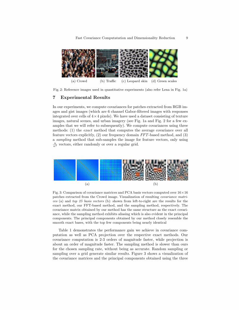
(a) Crowd (b) Traffic (c) Leopard skin (d) Green scales

Fig. 2: Reference images used in quantitative experiments (also refer Lena in Fig. 1a)

7 Experimental Results

In our experiments, we compute covariances for patches extracted from RGB im-ages and gist images (which are 6 channel Gabor-filtered images with responsesintegrated over cells of 4×4 pixels). We have used a dataset consisting of textureimages, natural scenes, and urban imagery (see Fig. 1a and Fig. 2 for a few ex-amples that we will refer to subsequently). We compute covariances using threemethods: (1) the exact method that computes the average covariance over allfeature vectors explicitly, (2) our frequency domain FFT -based method, and (3)a sampling method that sub-samples the image for feature vectors, only usingn

w2 vectors, either randomly or over a regular grid.

(a) (b)

Fig. 3: Comparison of covariance matrices and PCA basis vectors computed over 16×16patches extracted from the Crowd image. Visualization of resulting covariance matri-ces (a) and top 25 basis vectors (b): shown from left-to-right are the results for theexact method, our FFT-based method, and the sampling method, respectively. Thecovariance matrix obtained by our method has the same structure as the exact covari-ance, while the sampling method exhibits aliasing which is also evident in the principalcomponents. The principal components obtained by our method closely resemble thesmooth exact bases, with the top few components being nearly identical

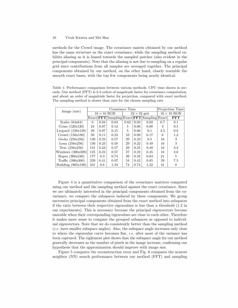
Table 1 demonstrates the performance gain we achieve in covariance com-putation as well as PCA projection over the respective exact methods. Ourcovariance computation is 2-3 orders of magnitude faster, while projection isabout an order of magnitude faster. The sampling method is slower than oursfor the chosen sampling rate, without being as accurate. Random sampling orsampling over a grid generate similar results. Figure 3 shows a visualization ofthe covariance matrices and the principal components obtained using the three


methods for the Crowd image. The covariance matrix obtained by our methodhas the same structure as the exact covariance, while the sampling method ex-hibits aliasing as it is biased towards the sampled patches (also evident in theprincipal components). Note that the aliasing is not due to sampling on a regulargrid since contributions from all samples are averaged together. The principalcomponents obtained by our method, on the other hand, closely resemble thesmooth exact bases, with the top few components being nearly identical.

Table 1: Performance comparison between various methods. CPU time shown in sec-onds. Our method (FFT) is 2-3 orders of magnitude faster for covariance computation,and about an order of magnitude faster for projection, compared with exact method.The sampling method is slower than ours for the chosen sampling rate

Image (size)Covariance Time Projection Time

16× 16 RGB 32× 32 gist 16× 16 RGBExact FFT Sampling Exact FFT Sampling Exact FFT

Scales (64x64) 6 0.04 0.04 0.62 0.02 0.02 0.7 0.1Grass (120x120) 24 0.07 0.12 5 0.06 0.08 3 0.5

Leopard (128x128) 29 0.07 0.15 5 0.06 0.1 3.5 0.6Crowd (150x180) 50 0.11 0.23 10 0.09 0.17 6 1.2Gecko (256x256) 130 0.23 0.57 29 0.23 0.5 16 3Lena (256x256) 130 0.23 0.59 29 0.22 0.49 16 3Text (256x256) 131 0.23 0.57 29 0.25 0.49 16 3.2

Windows (306x208) 125 0.23 0.57 27 0.22 0.45 16 3.6Ropes (360x240) 177 0.3 0.74 39 0.32 0.64 21 5Traffic (390x300) 239 0.41 0.97 54 0.42 0.85 29 7.5

Building (865x190) 341 0.6 1.34 74 0.74 1.22 41 8

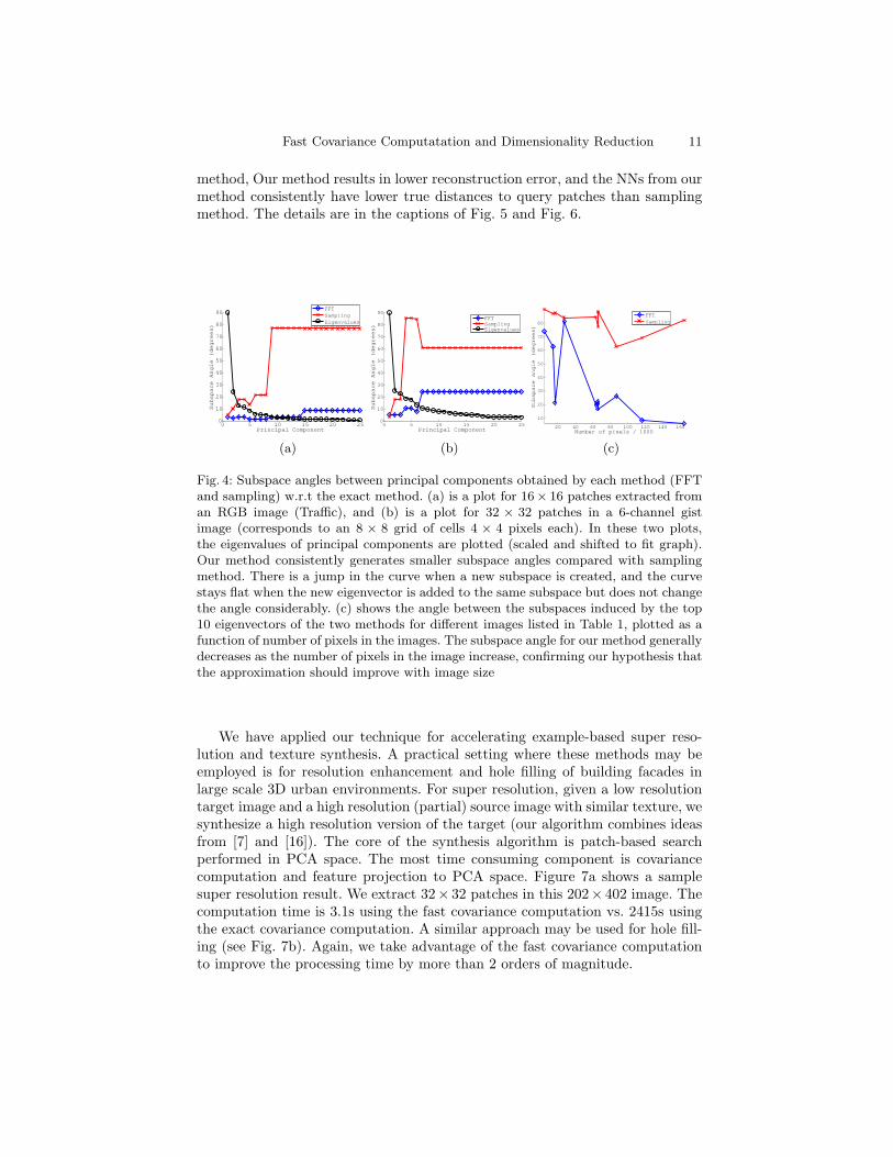
Figure 4 is a quantitative comparison of the covariance matrices computedusing our method and the sampling method against the exact covariance. Sincewe are ultimately interested in the principal components obtained from the co-variance, we compare the subspaces induced by these components. We groupsuccessive principal components obtained from the exact method into subspacesif the ratio between their respective eigenvalues is less than a threshold (1.2 inour experiments). This is necessary because the principal eigenvectors becomeunstable when their corresponding eigenvalues are close to each other. Thereforeit makes more sense to compare the grouped subspaces as opposed to individ-ual eigenvectors. Note that we do consistently better than the sampling method(i.e. have smaller subspace angles). Also, the subspace angle increases only closeto where the eigenvalue curve becomes flat, i.e. after most of the variance hasbeen captured. The rightmost plot shows that the subspace angle for our methodgenerally decreases as the number of pixels in the image increase, confirming ourhypothesis that the approximation should improve with image size.

Figure 5 compares the reconstruction error and Fig. 6 compares the nearestneighbor (NN) search performance between our method (FFT) and sampling


method, Our method results in lower reconstruction error, and the NNs from ourmethod consistently have lower true distances to query patches than samplingmethod. The details are in the captions of Fig. 5 and Fig. 6.

0 5 10 15 20 250

10

20

30

40

50

60

70

80

90

Principal Component

Subspace Angle (degrees)

FFTSamplingEigenvalues

(a)

0 5 10 15 20 250

10

20

30

40

50

60

70

80

90

Principal Component

Subspace Angle (degrees)

FFTSamplingEigenvalues

(b)

20 40 60 80 100 120 140 160

10

20

30

40

50

60

70

80

Number of pixels / 1000

Subspace angle (degrees)

FFT

Sampling

(c)

Fig. 4: Subspace angles between principal components obtained by each method (FFTand sampling) w.r.t the exact method. (a) is a plot for 16× 16 patches extracted froman RGB image (Traffic), and (b) is a plot for 32 × 32 patches in a 6-channel gistimage (corresponds to an 8 × 8 grid of cells 4 × 4 pixels each). In these two plots,the eigenvalues of principal components are plotted (scaled and shifted to fit graph).Our method consistently generates smaller subspace angles compared with samplingmethod. There is a jump in the curve when a new subspace is created, and the curvestays flat when the new eigenvector is added to the same subspace but does not changethe angle considerably. (c) shows the angle between the subspaces induced by the top10 eigenvectors of the two methods for different images listed in Table 1, plotted as afunction of number of pixels in the images. The subspace angle for our method generallydecreases as the number of pixels in the image increase, confirming our hypothesis thatthe approximation should improve with image size

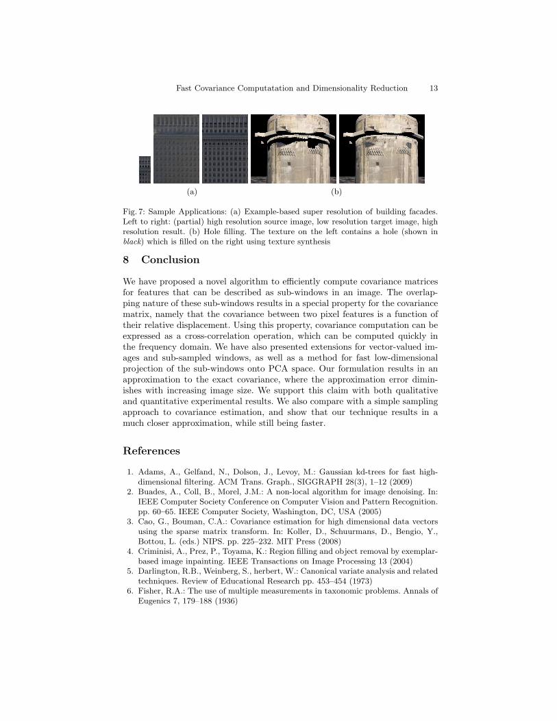
We have applied our technique for accelerating example-based super reso-lution and texture synthesis. A practical setting where these methods may beemployed is for resolution enhancement and hole filling of building facades inlarge scale 3D urban environments. For super resolution, given a low resolutiontarget image and a high resolution (partial) source image with similar texture, wesynthesize a high resolution version of the target (our algorithm combines ideasfrom [7] and [16]). The core of the synthesis algorithm is patch-based searchperformed in PCA space. The most time consuming component is covariancecomputation and feature projection to PCA space. Figure 7a shows a samplesuper resolution result. We extract 32× 32 patches in this 202× 402 image. Thecomputation time is 3.1s using the fast covariance computation vs. 2415s usingthe exact covariance computation. A similar approach may be used for hole fill-ing (see Fig. 7b). Again, we take advantage of the fast covariance computationto improve the processing time by more than 2 orders of magnitude.


(a) Traffic (b) Lena (c) Leopard skin (d) Green scales

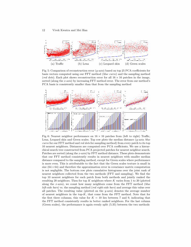
Fig. 5: Comparison of reconstruction error (y-axis) based on top 25 PCA coefficients forbasis vectors computed using our FFT method (blue curve) and the sampling method(red dots). Each plot shows reconstruction error for all 16 × 16 patches in the image,sorted (along the x-axis) by increasing FFT method error. The error from our method’sPCA basis is consistently smaller than that from the sampling method

Fig. 6: Nearest neighbor performance on 16 × 16 patches from (left to right) Traffic,Lena, Leopard skin and Green scales. Top row plots the median distance (y-axis; bluecurve for our FFT method and red dots for sampling method) from every patch to its top10 nearest neighbors. Distances are computed over PCA coefficients. We use a hierar-chical search tree constructed from PCA projected patches for nearest neighbor search.Patches are sorted (along the x-axis) by FFT method distance. These plots demonstratethat our FFT method consistently results in nearest neighbors with smaller mediandistance compared to the sampling method, except for Green scales where performanceis more even. This is attributable to the fact that the Green scales texture is small insize (64× 64) and therefore the approximation error in covariance matrix computationis not negligible. The bottom row plots cumulative histograms over the joint rank ofnearest neighbors collected from the two methods (FFT and sampling). We find thetop 10 nearest neighbors for each patch from both methods and jointly ranked theresulting 20 neighbors. Then for top K neighbors where K varies from 1 to 20 (plottedalong the x-axis), we count how many neighbors come from the FFT method (blueleft-side bars) vs. the sampling method (red right-side bars) and average this value overall patches. The resulting value (plotted on the y-axis) denotes the average numberof nearest neighbors in the top-K, that come from the FFT method. Note that forthe first three columns, this value for K = 10 lies between 7 and 9, indicating thatthe FFT method consistently results in better ranked neighbors. For the last column(Green scales), the performance is again evenly split (5.35) between the two methods


(a) (b)

Fig. 7: Sample Applications: (a) Example-based super resolution of building facades.Left to right: (partial) high resolution source image, low resolution target image, highresolution result. (b) Hole filling. The texture on the left contains a hole (shown inblack) which is filled on the right using texture synthesis

8 Conclusion

We have proposed a novel algorithm to efficiently compute covariance matricesfor features that can be described as sub-windows in an image. The overlap-ping nature of these sub-windows results in a special property for the covariancematrix, namely that the covariance between two pixel features is a function oftheir relative displacement. Using this property, covariance computation can beexpressed as a cross-correlation operation, which can be computed quickly inthe frequency domain. We have also presented extensions for vector-valued im-ages and sub-sampled windows, as well as a method for fast low-dimensionalprojection of the sub-windows onto PCA space. Our formulation results in anapproximation to the exact covariance, where the approximation error dimin-ishes with increasing image size. We support this claim with both qualitativeand quantitative experimental results. We also compare with a simple samplingapproach to covariance estimation, and show that our technique results in amuch closer approximation, while still being faster.

References

1. Adams, A., Gelfand, N., Dolson, J., Levoy, M.: Gaussian kd-trees for fast high-dimensional filtering. ACM Trans. Graph., SIGGRAPH 28(3), 1–12 (2009)

2. Buades, A., Coll, B., Morel, J.M.: A non-local algorithm for image denoising. In:IEEE Computer Society Conference on Computer Vision and Pattern Recognition.pp. 60–65. IEEE Computer Society, Washington, DC, USA (2005)

3. Cao, G., Bouman, C.A.: Covariance estimation for high dimensional data vectorsusing the sparse matrix transform. In: Koller, D., Schuurmans, D., Bengio, Y.,Bottou, L. (eds.) NIPS. pp. 225–232. MIT Press (2008)

4. Criminisi, A., Prez, P., Toyama, K.: Region filling and object removal by exemplar-based image inpainting. IEEE Transactions on Image Processing 13 (2004)

5. Darlington, R.B., Weinberg, S., herbert, W.: Canonical variate analysis and relatedtechniques. Review of Educational Research pp. 453–454 (1973)

6. Fisher, R.A.: The use of multiple measurements in taxonomic problems. Annals ofEugenics 7, 179–188 (1936)


7. Freeman, W.T., Jones, T.R., Pasztor, E.C.: Example-based super resolution. IEEEComput. Graph. Appl. (2002)

8. Fukunaga, K.: Introduction to Statistical Pattern Recognition, Second Edition(Computer Science and Scientific Computing Series). Academic Press (1990)

9. Higham, N.J.: Computing the nearest correlation matrix a problem from finance.IMA Journal of Numerical Analysis 22(3), 329–343 (2002)

10. Jain, A.K., Duin, R.P.W., Mao, J.: Statistical pattern recognition: A review. IEEETransactions on Pattern Analysis and Machine Intelligence 22(1), 4–37 (2000)

11. Jones, J.P., Palmer, L.A.: An evaluation of the two-dimensional gabor filter modelof simple receptive fields in cat striate cortex. J Neurophysiol 58(6), 1233–1258(December 1987)

12. Ke, Y., Sukthankar, R.: Pca-sift: a more distinctive representation for local im-age descriptors. In: IEEE Computer Society Conference on Computer Vision andPattern Recognition. vol. 2, pp. 506–513 (2004)

13. Kim, K.I., Franz, M., Schlkopf, B.: Kernel hebbian algorithm for single-framesuper-resolution. In: Leonardis, A., H.B. (ed.) Statistical Learning in ComputerVision. pp. 135–149. Springer, Berlin, Germany (2004)

14. Kim, K.I., Franz, M.O., Schlkopf, B.: Iterative kernel principal component analysisfor image modeling. IEEE Transactions on Pattern Analysis and Machine Intelli-gence 27(9), 1351–1366 (2005)

15. Korah, T., Rasmussen, C.: Pca-based recognition for efficient inpainting. In: IEEEAsian Conference on Computer Vision (2006)

16. Kwatra, V., Essa, I., Bobick, A., Kwatra, N.: Texture optimization for example-based synthesis. ACM Trans. Graph., SIGGRAPH 24(3), 795–802 (2005)

17. Lefebvre, S., Hoppe, H.: Appearance-space texture synthesis. In: Proc. of SIG-GRAPH ’06. pp. 541–548 (2006)

18. Lefebvre, S., Hoppe, H.: Parallel controllable texture synthesis. In: ACM Transac-tions on Graphics, SIGGRAPH. pp. 777–786 (2005)

19. Liang, L., Liu, C., Xu, Y., Guo, B., Shum, H.Y.: Real-time texture synthesis bypatch-based sampling. ACM Trans. Graph. 20(3), 127–150 (2001)

20. Liu, J., Wu, F., Yao, L., Zhuang, Y.: A prediction error compression method withtensor-pca in video coding. In: MCAM. pp. 493–500 (2007)

21. Oliva, A., Torralba, A.: Building the gist of a scene: the role of global image featuresin recognition. Progress in brain research 155, 23–36 (2006)

22. Pearson, K.: On lines and planes of closest fit to systems of points in space. Philo-sophical Magazine 2(6), 559–572 (1901)

23. Porikli, W.F., Tuzel, O.: Fast construction of covariance matrices for arbitrary sizeimage. In: Proc. Intl. Conf. on Image Processing. pp. 1581–1584 (2006)

24. Qi, J., Leahy, R.M.: Fast computation of the covariance of map reconstructions ofpet images. Proceedings of SPIE 3661(1), 344–355 (1999)

25. Stein, C., Efron, B., Morris, C.: Improving the usual estimator of a normal covari-ance matrix. Dept. of Statistics, Stanford University, Report 37 (1972)

26. Wang, Q., Tang, X., Shum, H.Y.: Patch based blind image super resolution. In:ICCV (2005)

27. Wei, L.Y., Lefebvre, S., Kwatra, V., Turk, G.: State of the art in example-basedtexture synthesis. In: Eurographics 2009, State of the Art Report, EG-STAR. Eu-rographics Association (2009)

28. Yu, Y.D., Kang, D.S., Kim, D.: Color image compression based on vector quan-tization using pca and lebld. In: Proc. of the IEEE Region 10 Conference. vol. 2,pp. 1259–1262 (1999)

Documents

Fast Covariance Computation and Dimensionality Reduction