Fair Matching Algorithm: An Optimal Scheduling Algorithm forthe AAPN network

AAPN Technical Report 2004-5

Nahid Saberi and Mark J. CoatesDepartment of Electrical and Computer Engineering

McGill University

Sept. 2005

Abstract

The internal switches in all-photonic networks do not perform data conversion into the electronic domain,thereby eliminating a potential capacity bottleneck, but the inability to perform efficient optical bufferingintroduces network scheduling challenges. In this technical report we focus on the problem of schedulingfixed-length frames in all-photonic star-topology networks with the goal of minimizing rejected demand.We describe the Fair Matching Algorithm, a novel scheduling technique for fixed-length frames. FMAguarantees 100% throughput provided the arrivals to the network induce an admissible demand matrix,and results in an allocation that is weighted max-min fair. We compare through OPNET simulation thedelay and throughput performance of FMA with the less computationally-complex Minimum Cost Searchalgorithm. We also describe the Minimum Rejection Algorithm (MRA), which minimizes total rejection,and demonstrate that the Fair Matching Algorithm (FMA) minimizes the maximum percentage rejection ofany connection. We analyze through simulation the rejection and delay performance.

1 Introduction

Electronic switches in high-speed networks are increasingly proving to bea capacity bottleneck. Replace-ment with all-photonic switches is attractive, particularly as photonic devices with sub-microsecond switch-ing capability become available. The inability of the photonic switches to performqueuing introduces net-work design challenges. Control functionality is required to reduce or eliminate the potential of contentionfor egress ports. Burst switching and just-in-time reservation approaches [1], and routing and wavelengthassignment techniques [2], are some of the many approaches that have been used in general mesh topolo-gies. An alternative approach is to focus on a simpler architecture that reduces the complexity of the controlchallenge.

Figure 1. Architecture of the Agile All-Photonic Network described in [3, 4]. Edge nodes performelectronic-to-optical conversion and transmit scheduling requests to the core photonic node(s). Selec-tors/multiplexor devices are used to merge traffic from multiple sources onto single fibres and to extracttraffic targetted to a specific destination. The structure forms an overlaid star topology (see Figure2).

In this research, we focus on the overlaid star topology, as specified in the design for the agile all-photonic network (AAPN) architecture of [3, 4]. This architecture (seeFigure 1) consists of edge nodes,where the optical electronic conversion takes place, connected via selector/multiplexor devices to photoniccore crossbar switches. The overlaid star topology facilitates the introduction of various approaches to time-sharing link capacity and dramatically reduces the complexity of the control problem. The core switchesact independently, so the control problem becomes one of scheduling theswitch configurations to achieve agood match with the traffic arrival pattern at the edge nodes.

The star topology also makes the introduction of accurate network-wide synchronization much morefeasible [5], and this enables the application of a range of Optical Time Division Multiplexing (OTDM)techniques for sharing link and switch capacity. A source edge-node must be aware of when it has ownershipof a given time-slot and is allowed to transmit to a specific destination edge node. By suitably allowing forthe differing propagation delays between various edge nodes and the core, time slots arrive at the corecrossbar switch at the same time and can be switched to their appropriate destinations without output portcollisions.

The slot allocation can be fixed and deterministic, or it can adapt to the trafficarrivals through signalling

1

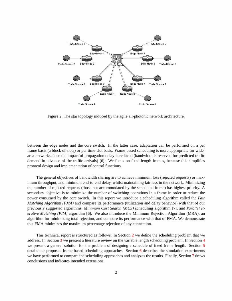
Figure 2. The star topology induced by the agile all-photonic network architecture.

between the edge nodes and the core switch. In the latter case, adaptation can be performed on a perframe basis (a block of slots) or per time-slot basis. Frame-based scheduling is more appropriate for wide-area networks since the impact of propagation delay is reduced (bandwidth is reserved for predicted trafficdemand in advance of the traffic arrivals) [6]. We focus on fixed-length frames, because this simplifiesprotocol design and implementation of control functions.

The general objectives of bandwidth sharing are to achieve minimum loss (rejected requests) or max-imum throughput, and minimum end-to-end delay, whilst maintaining fairness in thenetwork. Minimizingthe number of rejected requests (those not accommodated by the scheduledframe) has highest priority. Asecondary objective is to minimize the number of switching operations in a frame inorder to reduce thepower consumed by the core switch. In this report we introduce a scheduling algorithm called theFairMatching Algorithm (FMA)and compare its performance (utilization and delay behavior) with that of ourpreviously suggested algorithms,Minimum Cost Search (MCS)scheduling algorithm [7], andParallel It-erative Matching (PIM)algorithm [6]. We also introduce the Minimum Rejection Algorithm (MRA), analgorithm for minimizing total rejection, and compare its performance with that of FMA. We demonstratethat FMA minimizes the maximum percentage rejection of any connection.

This technical report is structured as follows. In Section2 we define the scheduling problem that weaddress. In Section3 we present a literature review on the variable length scheduling problem. InSection4we present a general solution for the problem of designing a schedule of fixed frame length. Section5details our proposed frame-based scheduling approaches. Section6 describes the simulation experimentswe have performed to compare the scheduling approaches and analyzesthe results. Finally, Section7 drawsconclusions and indicates intended extensions.

2

2 Fixed Frame Length Scheduling: Problem Definition

The AAPN architecture is an overlaid star-topology ofN edge nodes that operates over multiple wave-lengths [4]. It permits each node to transmit to one destination node and receive from one source nodesimultaneouslyon each wavelength. We consider that (flow-based) load balancing has been conducted todivide incoming traffic amongst the various stars. The remaining task is to schedule the traffic for each star.We are presented with a demand matrixD, whereDij is the number of slots requested by source nodeifor destinationj during the next fixed-length frame. We consider a frame of lengthF time slots withWavailable wavelengths, such that there areL = FW slots for each destination node available for allocation.Herein we focus on the case whereW = 1 for clarity, but the algorithms and results are easily extended.

We are presented with a demand matrixD, whereDij is the number of slots requested by source nodeifor destinationj during the next fixed-length frame. We define the followingline sumsof the demand matrix.Therow-sum, ri(D) =

∑Nj=1 Dij , is the total demand at sourcei, and thecolumn-sum, cj(D) =

∑Ni=1 Dij ,

is the total demand for destinationj. It is important to achieve zero rejection if the demand isadmissible.

Definition 1. A demand matrixD is admissibleif

max{maxi{ri(D)}, max

j{cj(D)}} ≤ L, (1)

whereL is the frame-length, andri(D) andcj(D) are thei-th row-sum andj-th column-sum of the demandmatrix, respectively.

Our aim is to devise a scheduleS such that the elementSjk identifies the source node allocated tothe k-th time slot associated with destinationj in the frame. The schedule should minimize the numberof rejectionsREJ(S, D, L) whilst also attempting to minimize the number of times that the switch mustreconfigure,Ns(S). A switch reconfiguration occurs between two consecutive time slotsk andk + 1 if theallocated source node to any destinationj is altered;Ns(S) counts the number of switch reconfigurations inthe entire schedule, not merely those within the frame.

The number of rejections is defined as:

REJ(S, D, L) =∑

i

∑

j

max(0, Dij −

L∑

k=1

I[Sjk = i]), (2)

whereI is the indicator function. We can define an objective function (the cost of transmission) as:

C(S, D, L) = REJ(S, D, L) + g . Ns(S) , (3)

whereg is a constant that determines the relative importance of reducing the number of switch reconfigura-tions.

We identify two scheduling problems that address bandwidth allocation in an AAPN:PROBLEM 1:For an admissible demand matrixD and frame of lengthL, generate a scheduleS that

achieves zero rejection,REJ(S, D, L) = 0, and allocates spare capacity in the network to the connectionsin a (weighted) max-min fair manner.

PROBLEM 2:Solve the following optimization problem for a frame of fixed lengthL with C(S, D, L)defined by (3) to identify a frame schedule.

S∗1 = arg min

SC(S, D, L) (4)

3

The most closely related work to the optimization embodied inPROBLEM 1andand PROBLEM 2isthe problem of finding an optimum schedule for a variable-length frame, which has been extensively studiedin WDM and satellite systems [8–12]. The goal is to minimize the overall transmissiontimeT :

T (S) = Tx(S) + τ . Ns(S), (5)

whereNs is the number of switch reconfigurations,τ is the switching time, andTx is the time spent trans-mitting the traffic [9,11]. The minimum traffic transmission timeT ∗

x = max{maxi{ri}, maxj{cj}} [13].All times are measured in slots.

PROBLEM 3: Solve the following optimization problem for a frame of variable length with totaltransmission timeT (S) defined by (5), observing the constraint thatS ∈ S, the set of schedules that satisfythe demand matrix, i.e.,REJ(S, D, Tx(S)) = 0.

S∗2 = arg min

S∈ST (S) (6)

PROBLEM 3is NP -hard for non-negligible values ofτ [11, 14]. Crescenzi et al. demonstrate thatit cannot be approximated by a polynomial algorithm within a factor less than7

6 [14]. For small valuesof τ the problem can be closely approximated by the minimization ofTx, which is solvable in polynomialtime [15–17]. The minimum traffic transmission time is [13]:

T ∗x = max{max

i{ri}, max

j{cj}}.

We can then establish:

Claim 1. A scheduleSx that minimizes the traffic transmission time, i.e.,Tx(Sx) = T ∗x , solves PROBLEM

3 to within an approximation factor of1 + τ .

Proof. The number of switch reconfigurationsNs(S) < Tx(S) andT (S∗2) = Tx(S2) + τNs(S2) > T ∗

x .Hence ifSx minimizes the traffic transmission time, it satisfiesT (Sx) < T ∗

x (1 + τ) < T (S∗2)(1 + τ).

For the special case of smallτ , approximate algorithms that attempt to minimizeNs subject to theconstraint thatTx is minimum have been proposed in [8,9,12,14]. The algorithms achieve minimumtraffictransmission time,T ∗

x , but do not guarantee minimumtotal transmission time,T (S∗2), unless the switching

overhead is completely neglected. TheEXACTalgorithm, presented in [12,14], achieves a minimum traffictransmission time,T ∗

x and the derived schedule has at mostNs = N2 − 2N + 2 switch configurations [12].In the case of an admissible demand matrix, theEXACTalgorithm generates a scheduleS that has lengthless thanL and therefore zero rejection. TheEXACTalgorithm is an iterative procedure that repeatedlyperforms maximum cardinality bipartite matching (MCBM) to obtain the schedule. Itlies at the heart of thealgorithms we present in this report for the case of fixed-length frames.

Whenτ is very large (on the order of maximum transmission time), the problem is reduced to mini-mizingTD subject to the constraint thatNs is minimum. Approximate algorithms for this special case havebeen proposed in [9, 11]. The intermediate scenario, when it is desirableto obtain near minimum solutionsfor both the number of switchings and the traffic transmission time, has been addressed in [12].

4

3 Literature review

Depending on the value ofτ the problem of finding a minimum schedule length given by equation5 isusually reduced to the three following cases.

1) Whenτ is negligible compared to the duration of a time slot, the problem is reduced to the problemof minimizing TD, which has been studied in [15–17]. This problem can be solved in polynomial time. Ina more precise manner the problem can be reduced to minimizingNs subject to the constraint thatTD isminimum [8,9].

2) Whenτ is very large (in the order of minimum transmission time), the problem is reduced tomini-mizingTD subject to the constraint thatNs is minimum [9,11].

3) Whenτ is moderately large, it is more desirable to obtain near minimum solutions for both thenumber of switchings and the traffic transmission time [12]. In [14] it is shownthat one cannot approximatethis problem within a factor less than76 .

The three problems stated above have been formulated as variants of openshop scheduling problem inliterature [10–13,18].

3.1 Open Shop Formulation

First, we describe a scheme for classifying scheduling problems developed by Graham et al. [19]. SupposethatM machines or processorsPk (k = 1, ..., M) have to processN jobsJi (i = 1, ..., N). A scheduleis an allocation of one or more machines to each job. A schedule isfeasibleif at any time, there is at mostone job on each machine, each job is run on at most one machine, and it satisfies a number of requirementsconcerning the machine environment and the job characteristics. A schedule is optimum if it minimizes (ormaximizes) a given optimality criterion.

A shop scheduling problem consists of a set ofM processors. Each of these processors performs adifferent task. There areN jobs, each consisting ofM tasks. Each taskj of job i denoted byti,j is to beprocessed on processorj for a total duration ofdur(ti,j). In each time the following restrictions must besatisfied for the machines and the jobs: (i) each machine can execute at mostone task at any given time, and(ii) for each job at most one task is to be assigned. Depending on the orders by which the jobs and the tasksshould be performed the shop scheduling problem is usually classified to three basic groups:

1. When there is no ordering constraints on operations of the jobs the scheduling is described as anopenshop scheduling.

2. When operations of the tasks of each job should follow a specific orderthe shop scheduling is calledjob shop.

3. When every job goes through allM machines in a unidirectional order the shop scheduling isflowshop. Each job has exactlyM tasks. The first task of every job is done on machine 1, second task onmachine 2 and so on. However, the processing time each task spends on a machine varies dependingon the job that the task belongs to.

When the shop isopen the jobs and tasks can be executed in any order. The scheduling algorithmscanbe designed for two different categories based on how the tasks deal with interruption: preemptiveand

5

nonpreemptiveschedules. A preemptive schedule is the one which does not restrict the tasks to be executedcontinuously. A nonpreemptive schedule is the one in which the tasks can not be interrupted once they havebegun execution [9].

For a given open shop problem, we try to obtain an optimal finish time (OFT). AnOFT minimizesthemakespan or the time required to complete all the jobs. In general apreemptive open shopproblemcan be solved in polynomial time, while a nonpreemptive open shop problem is shown to beNP -hard1 [11] for more than three machines [13,20], but many heuristics exist to obtain near-optimal finish time forthis case [21, 22]. The open shop scheduling problem of N jobs and M machines is denoted byN | M |openshop | OFT [9].

3.2 Analogy

The scheduling problem for anN×N optical switch can be translated into an open shop scheduling problemwith M = N processors andN jobs. The jobs correspond to the inputs of the switch and the processorscorrespond to the outputs. Each input-output traffic demand,Dij , is represented by a taskti,j . Similarto the open shop formulation each task,Dij , belongs to a specific job (inputi) and is to be processed bya specific processor (outputj) [9]. The scheduling problem obtained isN | N | open shop| OFT. Thescheduling constraint in an optical switch operating on one wavelength canbe translated directly to the openshop scheduling. The constraint in an optical switch is that at each giventime (i.e., a time slot) at most onerequest from inputi can be serviced at each outputj:• One assignment of each input per slot is equivalent to the constraint thata job can not be processed bymore than one processor at any given time.• One assignment of each output per slot is equivalent to the constraint that a processor can perform at mostone task at any given time [9].

3.3 Scheduling Algorithms

In this section we describe several solutions for open shop scheduling problem which have been designedfor satellite systems and passive star networks. We develop the algorithms for an N × N nonblockingoptical switch. The first group of the algorithms aim at minimizing the number of switchings for a minimumduration schedule [8,9]. The second group of the algorithms try to minimize theschedule length when thenumber of switchings is minimum [9, 11]. The third group of algorithms provide near-optimum solutionswith bounds on the number of switchings and the schedule length [12].

3.3.1 Minimal Duration Scheduling

The problem of finding a schedule with minimum duration has been studied in manyresearch areas such asnetworks, computers, and satellite systems [8, 9, 12, 17], and was shownto be solvable in polynomial time.The algorithms achieve a minimum traffic transmission time,TDmin

, but the minimum schedule length,Tmin, for non-negligible switching overhead is not guaranteed. In this sectionwe present a simple algorithmwhich obtains at mostNs = N2 − 2N + 2 switch configurations per port [12]. However, this algorithmis a pseudopolynomial time algorithm not a polynomial-time one [14]. A similar algorithm proposedin [9,13] overcomes the problem noted above by obtaining a weight-regular graph from the original one. A

1A problem is NP-hard if solving it in polynomial time would make it possible to solve all problems in class NP in polynomialtime.

6

weight-regular graph is defined as a graph whose vertices have the samenumber of incident edges. Anotheralgorithm proposed by Pomalaza [10], tries to reduce the number of switchings by the weight matchingalgorithm. All of these algorithms assume that the assignments for each demand do not need to be continues,which translates our scheduling problem to solving apreemptive N | N | openshop | OFT problem.

Given a set of N jobs with task timesDij , 1 ≤ i ≤ N and1 ≤ j ≤ N , for anN -processor open shopproblem, we define the following quantities:

ri =∑

1≤j≤N

Dij = length of job i,

cj =∑

1≤i≤N

Dij = total time needed on processor j,

(7)

whereri, is the amount of the demand at inputi, andcj is the total demand for outputj. It is easily under-stood thatTDmin

= max{maxi{ri}, maxj{cj}} (the maximum Line-sum in the traffic matrix ).

Before describing the algorithms, we review some terminology and fundamental definitions concern-ing bipartite graphs. The following definitions are presented from [13,23].

Definition 2. A graphG is a pairG = (Y, E) whereY is a finite set of nodes or vertices and the elements inE consist of subsets ofY of cardinality two called edges. Ife = [v1, v2] ∈ E, then we say thate is incidentuponv1 (andv2). The degree of a vertexv of G is the number of edges incident uponv.

Definition 3. A graphG in which each edge has been assigned a number, or a weight, is called a weightedgraph. In a weighted graph, the weight of a vertexv is defined as the sum of the edge weights of all edgesincident tov in graphG.

Definition 4. Let G = (Y, E) is a graph that has the following property: the set of verticesY can bepartitioned into two sets,V andU , and each edge inE has one vertex inV and one vertex inU . ThenG iscalled a bipartite graph and is usually denoted byG = (V ∪U, E). Figure3-(a) shows a bipartite graph of8 vertices and 9 edges.

Definition 5. Let G = (V ∪ U, E) be a bipartite graph with vertex setsV andU , and edge setE. A setI ⊆ E is a matching if no vertexw ∈ V ∪ U is incident with more than one edge inI. A matching ofmaximum cardinality is called amaximum matching. A matching is called acomplete matching (orperfect matching ) ofV into U if the cardinality (size) ofI equals the number of vertices inU . Figure3-(b)shows a matching of maximum cardinality obtained from the graph of figure3-(a).

Definition 6. An augmenting pathP relative to a matchingM in G is a path inG such that the first and thelast vertices inP are not covered byM , and the edges inP alternate between being inM and not being inM .

7

e7

e5

e3

e6

v1 v5

v4

v3

v2

v8

v7

v6

e4

e7

e5

e3 e1

e2

e6

e

8

e9

v1 v5

v4

v3

v2

v8

v7

v6

(a) (b)

Figure 3. (a) A bipartite graph of 8 vertices and 9 edges. (b) A matching ofmaximum cardinality obtainedfrom the bipartite graph. This matching is a perfect matching.

Note: If there exists such an augmenting path it can be proved that a matching of greater cardinalitycan be found inG by augmentingM with augmenting pathP . Consequently, a matching is of maximumcardinality if and only if it permits no augmenting path [23].

Definition 7. The degree of a graphG = (Y, E) is defined as the maximum degree of all its vertices. Forexample in figure3-(a) the degree of the graph is 3.

Maximum Cardinality Matching Algorithm for Bipartite Graph (MCB):The algorithm starts with anarbitrary matching Q in graph G. An augmenting path P with respect to Q is found. Then a new matchingis constructed by taking those edges of Q or P that are not in both Q and P. The process is repeated and thematching is maximal when no augmenting path is found.

EXACT Covering Algorithm. TheEXACTalgorithm, presented in [12,14], is based on finding the max-imum cardinality matching in bipartite graphs. We construct a bipartite graphG = (V ∪ U, E), whereVis the set of vertices corresponding to theN jobs (inputs of the optical switch),U is the sets of verticescorresponding to theN processors (outputs of the optical switch), andE is the set of edges incident toeach input-output pair. The algorithm repeatedly performs maximum cardinality matching on the nonzeroelements of the traffic matrixD. The weight of each matching, which corresponds to each configuration, isequal to the minimum weight of the edges participating in the matching. The weight of each edge (vi, uj) isthe amount of the requested traffic from inputi to outputj.

8

Algorithm EXACT.

%initializationi = 1, A = Dcreate graphG = (V ∪ U, E) from A% find a maximum matchingM of this graph using algorithm MCBwhile A ! = 0;

M = MCB(V ∪ U, E);

% schedule constructionP (i) = M ; %construct a permutation matrixw(i) = min{w(e) : e ∈M};%update the graphA = A− w(i)p(i);%update the graphA = A− w(i)p(i);i=i+1;%finish when all of the elements inA are zero

end

It has been shown in [12, 17] that at mostNs = N2 − 2N + 2 switch configurations are necessaryto cover the traffic matrix. However, this approach provides apseudopolynomial-time algorithm, since itsrunning time depends linearly on the weights ofG [14]. In [9, 13] a similar algorithm, namely CompleteMatching Algorithm (CMA) has been proposed which obtains the schedule ina polynomial time. In thisapproach the bipartite graph is constructed usingN + M real nodes andN + M fictitious nodes. Theidea is to make each processor to have the same load (TDmin

), and each job to have the same processingrequirement (TDmin

), hence obtaining a weight-regular graph, that is, a graph whose vertices have equalweights. A weight-regular graph guarantees the existence of a complete matching. With complete matchingsit is guaranteed that all processors are being used and all jobs are being processed in each iteration [13].Therefore it can be proved that the algorithm CMA always produces a minimum length schedule of durationTDmin

[9, 13]. The time complexity of this algorithm isO(‖V ‖‖E‖) where‖V ‖ and‖E‖ are the numberof vertices and the number of edges in the Bipartite graph respectively. The size of a maximum cardinalitymatching, and thus the maximum number of iterations required to compute it, isO(‖V ‖), and the complexityof a graph search procedure isO(‖E‖).

Using parallel processing methods, the fastest known algorithm has a complexity of O(√

‖V ‖ ‖E‖)[24]. This algorithm reduces the number of iterations fromO(‖V ‖) to O(

√

‖V ‖), by looking for a set ofdisjoint M-augmenting paths per iteration, then augmenting along all the discovered paths. In other words,the algorithm runs the search procedure from all unmatched vertices simultaneously rather than one by one.

3.3.2 Minimum Number of Switchings

Recall that the objective function to minimize the overall transmission time isT = τNs + TD, whereτ isthe switching overhead,TD is the traffic transmission time, andNs is the number of switchings that mightbe taken to cover the traffic demand. Algorithms described in this section givea schedule with minimum

9

number of switchings. The algorithms aim at minimizingTD subject to the constraint thatNs is minimum.The problem in this case is formulated as anonpreemptive open shopscheduling problem. Nonpreemptivescheduling guarantees that the minimum number of switchings is always obtained. In [25] it has been provedthat minimizing the makespan (total transmission time) in a nonpreemptive open shopscheduling problemwhenM > 2 isNP -complete, whereM is the number of processors (for anN ×N switchM = N ).

The minimum number of switchings is determined by:

Nsmin= max{maxi{‖ri‖}, maxj{‖cj‖}}, (8)

where‖ri‖ is the number of nonzero entries in rowi and‖cj‖ is the number of nonzero entries in columnj.

Nonpreemptive Open shop Scheduling Algorithm. The algorithm presented in [9] is based on the mostnumber of tasks (demands) first heuristic. The algorithm starts by the output which is requested by thelargest number of inputs. At a given time slot if thej-th output is available and the inputsi andk are free, ifthe total number of tasks of inputi is greater than the total number of tasks of inputk, then the demandDij

is processed before the demanddk,j . Recall that the total number of tasks of inputi is the total number ofoutputs for which inputi has requests (the number of nonzero entries in rowi of a demand matrix). If thetotal number of tasks of inputi is equal to the total number of tasks of inputk, and if the total number ofrequests by inputi is smaller than the total number of requests by inputk, thenDij is processed before thedemanddk,j . The total number of requests by inputi is the sum of the total demands requested by inputi.This algorithm always produces the minimum number of switching matrices.

3.3.3 Near-Optimum Solutions

The algorithms described in sections3.3.1and3.3.2provide solutions for reducing the number of switch-ings and the transmission time respectively, but there is no guarantee on the performance of the proposedalgorithms when the amount ofτ is neither negligible nor very large. Using the proof described in [23] it canbe shown that the algorithm described in3.3.2has an unbounded approximation ratio for the transmissiontime. On the other hand the algorithms described in3.3.1provide the minimum traffic transmission time,but there is not a tight bound on the number of switchings. Consequently, the overall transmission time forthe case that the switching overhead is not negligible is not close to optimal.

In [14] this problem is described as the preemptive bipartite scheduling andshown to beNP -hardusing the proof in [11]. Also it is shown that one cannot approximate this problem within a factor less than76 , but the best algorithm they proposed approximates this problem within a factor of 2.

The approximation algorithm described in this section does not restrict the optimal schedule lengthor the minimum number of switchings. Instead, by allowing twice as many as the minimumnumber ofswitchings, it achieves a near-optimum schedule length within a ratio of two.

Graham’s List Scheduling. List scheduling (LIST) introduced by R. L. Graham [18] is a greedy algo-rithm2 that approximates the optimal open shop problem within a ratio of two. LIST starts by assigning a jobto each processor. If multiple jobs are contending for the same processorone of them is chosen arbitrarily.Once a processor is idle, one of the free jobs which has a task for the corresponding processor is chosenarbitrarily. This procedure continues until all of the jobs are processed.

2A greedy algorithm is an algorithm that optimizes the choice at each stage without regard to previous choices, with the hopeof finding the global optimum.

10

The maximum schedule length produced by LIST is bounded by the sum of thetime to process thelongest job (equal to the maximum row-sum in the traffic demand), and the time that the most heavily loadedprocessor needs (equal to the maximum column-sum in the traffic demand) [26]. Therefore this algorithmtends to a delay overhead of at most2τNsmin

, though the number of switchings at each port isNsmin.

4 Fixed Frame Length Scheduling

4.1 Terminology and Definitions

We now define some terminology that will be used throughout the report andrecall some definitions. Wedenote the line-sum of lineof the demand matrixD by LS`. Note that line consists of a set of source-destination demands (connections). Each of these connections belongs totwo lines (a row and a column).Thei-th row represents a link from sourcei to the optical switch at the core, and thej-th column representsthe link from the core to destination nodej.

For an inadmissible demand matrix, we denote the set of overflowing rows of the demand matrix (rowswith ri(D) > L) asOr, and the set of overflowing columns (cj(D) > L) asOc. The set of overflowinglines, O` = {` : LS` > L} is the union ofOr andOc. We define acritical connection, or criticaldemand element, as any demand entryDhp such thath ∈ Or andp ∈ Oc. The remaining entries constitutenon-criticalconnections/demands.

We now recall the definitions offeasibilityof rate allocation andweighted max-min fairness[27,28].

Definition 8. Feasibility: Consider an arbitrary network as a set of linksL where each link ∈ L has acapacityC` > 0. Let{1, · · · , ζ} be the set of connections in the network. LetDu be the demand (request)of connectionu andυu be its assigned rate. We call a rate allocation{υ1, υ2, · · · , υζ} feasible, when forevery link` we have:

∑

u∈H`

υu ≤ C` ∀` ∈ £. (9)

Definition 9. Weighted max-min fairness: Let ωu(υu) be an increasing function representing the weightsassigned to connectionu at rateυu. An allocation{υ1, υ2, · · · , υζ} is weighted max-min fairif for eachconnectionu any increase inυu would cause a decrease in transmission rate of connectionz satisfyingωz(υz) ≤ ωu(υu). The special case of max-min fairness is obtained byωu(υu) = υu.

Definition 10. Bottleneck Link: Given a feasible rate vectorυ and a weight vectorω, we say that link isa bottleneck linkwith respect to (υ , ω) for a connectionu crossing`, if C` =

∑

k υk , F` andωu ≥ ωk

for all connectionsk crossing .

Lemma 1. A feasible rate vectorυ with weight vectorω = { υu

Ru} is weighted max-min fair if and only if

each connection has a bottleneck link with respect to (υ , ω).

See the Appendix (Section8.1) for a proof.

4.2 Relationship to Variable-Length Frame Scheduling

TheEXACTalgorithm, presented in [12,14], addresses schedule design for variable length frames, primarilyfor the case of negligibleτ , and achieves a minimum traffic transmission time,T ∗

x . Thus in the case of

11

admissible demand matrices, theEXACTalgorithm generates a scheduleS that has length less thanL andtherefore satisfies the first requirement ofPROBLEM 1. TheEXACTalgorithm is an iterative procedure thatrepeatedly performs maximum cardinality bipartite matching (MCBM) to obtain the schedule. It lies at theheart of the algorithms we present in this report for the case of fixed-length frames.

We establish two results concerning the complexity ofPROBLEM 1:

Claim 2. If the demand matrixD is admissible and contains no zero entries (for anN × N switch andframe of lengthL) then the EXACT algorithm provides a solutionSE to PROBLEM 2 such thatC(SE) <C(S∗

1) + g(N2 − 3N + 2).

Proof. Since the demand matrix is admissible,T ∗x < L. Hence the schedule devised byEXACTresults

in zero rejections,REJ(S, D, L) = 0. EXACTensures that the number of switch reconfigurations in thissolution is less thanN2 − 2N + 2. The minimum number of switch reconfigurations for any scheduleunder the constraint of no zero-entries in the demand matrix isN [25]. Hence the maximum discrepancy isN2 − 3N + 2.

Theorem 1. For large g, such thatg > max(||D||1 − L, 0), where||D||1 =∑

i

∑

j Dij , PROBLEM 2 isreduced to the problem of minimizingREJ(S, D, L) subject to the constraint thatNs(S) is minimized. Forthis range ofg, PROBLEM 2 isNP -hard.

See the Appendix (Section8.2) for a proof.

5 AAPN Scheduling Algorithms

In a practical scenario, although it is desirable to reduce power expenditure by minimizing the number ofswitchings, minimizing the number of rejections is far more important. Hence we address the schedulingproblem (PROBLEM 1) wheng is small. In this case, we can rewrite the problem as:MINREJ(D,L): For a frame of fixed lengthL with demand matrixD identify a frame scheduleS∗

1 thatsatisfies:

S∗1 = arg min

SREJ(S, D, L) (10)

In this section, we describe two algorithms for bandwidth reservation in the AAPN architecture thataddress fixed-length frame scheduling. The Fair Matching Algorithm minimizesthe maximum percentagerejection experienced by any demand, while the Minimum Rejection Algorithm minimizes the total rejection(that is, it provides a solution toMINREJ(D,L)).

5.1 Fair Matching Algorithm (FMA)

The EXACTalgorithm can be applied directly to the case of fixed length frames (Claim 2 states that itprovides a solution forPROBLEM 1wheng is small and demand admissible). When the demand matrixis inadmissible, the schedule determined by the EXACT algorithm must be truncated afterL time slots.This can lead to starvation of some source-destination traffic, and result inunfairness (such as substantiallydifferent average service times for traffic arriving at different nodes).

If the demand matrix is admissible, FMA incrementally assign additional demand to allelements untilone of the links reaches capacity (its line-sum is equal toL). At that point, the demand elements contributingto that line are clamped. Extra demand is then gradually added to the remaining elements in the matrix untilanother link (line) reaches its capacity and it too is clamped. The procedurereferred to as thewater-filling

12

procedure repeats until all lines have reached capacity . FMA assigns extra capacityin proportion to theoriginal demand.

This algorithm can be implemented by processing one line at a time. We first choose the most con-strained line (the line that would reach its capacity first under the water-fillingprocedure) and increase itsdemand to capacity. Then we choose the next most constrained line and increase its demand to capacity. Werepeat until all lines have reached capacity.

A similar procedure can be used for the case of an inadmissible demand matrix.In this case FMAidentifies the most overloaded line and reduces the demands on that line suchthat they sum to capacity (L).Demand reduction is proportional to the original demand, i.e. each adjusted demand experiences the samepercentage reduction. In subsequent iterations, FMA identifies the next most constrained line, taking intoaccount the effect of any previous adjustments, and clamps its demand to capacity. It repeats the processuntil no lines exceed capacity. When there are both overloaded and under-utilized lines, the overloaded linesare adjusted first.

Here we describe how FMA treats demands belonging to the adjustable lines in the setU` = {` :LS`(0) 6= L}, whereLS`(0) is the line sum of line at the beginning of calculations. We defineAD ⊆ U`

as the set of unmodified lines andBD ⊆ U` as the set of modified lines. InitiallyAD contains all lines inU` andBD is empty. Similarly, we definea` as the set of unmodified demands in line` andb` as the setof modified demands. Initially,a` contains all the demands andb` is empty. DefineSa`

,∑

(i,j)∈a`Dij

andSb`,

∑

(i,j)∈b`D

′

ij . We always haveSa`+ Sb`

= LS`, andD′

ij is obtained from the following lineadjustment:

D′

ij = Dij ×L− Sb`

Sa`

∀ (i, j) ∈ a` (11)

Note that when demandDij belongs to an overloaded line,L−Sb`

Sa`

< 1, and whenDij belongs to an

under utilized lineL−Sb`

Sa`

> 1. Define for each of line inAD the valueG` ,L−LS`

Sa`

.

Algorithm 1 FMAwhile AD 6= Ø do

Identify the line`∗ = arg min`∈ADG`.

Apply (11) to line `∗.Transfer ∗ fromAD toBD.Updatea` andb` for all lines` ∈ AD.Re-evaluateLS` for all lines inAD.Transfer linesγ with LSγ = L fromAD toBD.

end whileApply EXACTto bD′c to generateS.

The following theorem states that prior to rounding, FMA achieves weightedmax-min fair allocationof capacity (weighted relative to the original demand). See the Appendix (Section8.3) for the proof of thetheorem.

Theorem 2. FMA generates an adjusted demand matrixD′ with weighted max-min fair allocation, where

the weight isω(D′ij) =

D′

ij

Dij.

If the demand matrix contains zero entries, then an algorithm that adjusts requests multiplicatively(such as FMA) cannot always generate full utilization; there can benatural blockingbecause there is no

13

demand. We now present some properties of the demand matrixD′

= {D′

ij} obtained by Algorithm 1 priorto rounding.

Property1 Algorithm 1 guarantees full allocation of all links providedD contains no zero elements.

Property2 If there is no natural blocking the maximum total throughput of the network isobtained:∑

i

∑

j

D′

ij = N.L. (12)

Property3 The while-loop in Algorithm 1 hasO(N2) computational complexity in terms of the number ofedge nodes (2N iterations with a minimization overN elements in each iteration). The best currentimplementation of theEXACTalgorithm has complexityO(N

5

2 ), and hence this is also the complexityof Algorithm 1.

Property4 Algorithm 1 guarantees minimum rejection if no connections cross two different overloadedlinks, i.e., if the overloaded links correspond entirely to rows (input links) or entirely to columns(output links) ofD. In this case:

min(REJ) =∑

`

(LS` − L) ∀` ∈ O, (13)

whereO is the set of overflowing lines.

Define thepercentage rejectionas1 −D′

ij

Dij. Consider the set of demands that experience the highest

percentage rejection (i.e. the demands on the most overloaded line). Since the weightω is a monotoni-cally increasing function of allocated rateD′

ij , weighted max-min fairness implies that it is impossible toincrease the rate allocated to these demands (or decrease the maximum percentage rejection) without vi-olating feasibility. Decreasing the rejection of any of those demands requires increasing the rejection ofanother demand on the same line, and hence the maximum percentage rejection increases. We thus have thefollowing corollary:

Corollary 1. Subject to the capacity constraints, FMA generates a schedule that minimizes the maximumpercentage rejection experienced by any connection.

5.2 Equal Share Algorithm (ESA)

The water-filling procedure can be implemented by assigning equal amount of extra capacity to the con-nections passing underloaded lines. This approach is similar to the max-min fairrate allocation of ABRconnections in ATM networks proposed by Charney et. al [29]. Similarly the overloaded lines can be ad-justed by reducing equal amounts from the demands of the connections passing these lines. We define foreach line the valuesH` ,

L−LS`

|a`|, where|a`| is the cardinality ofa`.

The line with minimumH` is the most constrained line. Repeatedly the most constrained line is definedand the demands of its connections are adjusted. The demand adjustment we perform on each line is:

D′

ij = Dij +L− LS`

|a`|∀ (i, j) ∈ a` (14)

The following theorem states that prior to rounding, ESA achieves max-min fair allocation of capacity. Seethe Appendix (Section8.4) for the proof of the theorem

Theorem 3. ESA generates an adjusted demand matrixD′ with max-min fair allocation of extra-capacity,where the weight of the connection between sourcei and destinationj is ωij = Dij −D′

ij .

14

5.3 Minimum Cost Search Algorithm

This section reviews an alternative approach, the minimum cost search (MCS) algorithm, which we firstdescribed in [7]. In order to reduce signalling overhead and to reducescheduling complexity, the algorithmsatisfies the transparency property [30]. This requires that the scheduling is only modified for new requestsor tear-downs (ifDij decreases or increases).

The minimum cost search algorithm we propose does not achieve optimal utilization, because it doesnot consider the global allocation problem; instead it allocates requests sequentially on a single time slotbasis. The algorithm operates by repeatedly visiting the(i, j) entries in the traffic demand matrixD ina round-robin fashion; at each visit, if the requested number of slots hasnot yet been assigned, the algo-rithm attempts to allocate a single time slot to the(i, j) request. The round-robin allocation results in anapproximately fair assignment of slots to each pair.

In order to determine which slot to allocate to the request, we define acostfor the allocation of a(i, j)source-destination pair to a time slot pairtk for k in 1, . . . L. This cost is determined entirely by the extant,partial frame schedule. The cost function is:

Cij(tk) = Nfs(tk) + λKij(tk), (15)

whereNfs(tk) is the number of free sources at this time slot, i.e., the number of sources not transmitting toany other destinations,λ is a small positive constant, andKij(tk) = {0, 1, 2} is the number of additionalswitching operations that the core switch must perform to accommodate the allocation. The motivationbehind this cost function is simple. The first term represents the current flexibility of that time slot (thenumber of free sources for future allocation) and reflects the desirabilityof retaining flexibility by allocatingdemands to the most constrained slots where possible. The second term reflects the desirability of minimiz-ing the power consumption of the optical switch, which is partially determined by the number of switchingoperations that it must perform each frame.

The scheduling of a single(i, j) time slot request is performed by first identifying the(i, j)-eligibleslots in the frame, which are defined as the free time slots during whichi is not transmitting to any otherdestination andj is not receiving from another source. The costCij(tk) of each of these eligible timeslots is evaluated, and the demand is assigned to the slot incurring minimum cost. In the case of ties, thedemand is assigned to the earliest slot and the lowest wavelength (assuming wavelengths are ordered insome fashion). Deallocation is implemented by a reverse procedure, in whichwe seek and release the mostcostly currently-allocated time slot. This algorithm has a worst case time complexityof O(N.L). (greennumbers)

5.4 Minimum Rejection Algorithm

In this section we describe an algorithm that generates a schedule that minimizes total rejection. We firstdevelop a theorem that helps to identify a procedure for solvingMINREJ(D,L). We commence by definingMAXFLOW(D,X,L), a max-flow linear programming problem.

Problem Y = MAXFLOW(D,X,L) : D is a demand matrix,X is a non-negative matrix that specifies capac-ity bounds, andL is the frame-length (available capacity on each row/column). MatricesD, X andY areall of sizeN ×N . Identify a nonnegative matrixY such that

∑

h∈Or

∑

p∈OcYhp is maximized, subject to

15

the following constraints:

Yhp = 0 if h /∈ Or or p /∈ Oc

Yhp ≤ Xhp ∀ (h, p) s.t. h ∈ Or and p ∈ Oc∑

p∈ Oc

Yhp ≤ rh(D)− L ∀ h ∈ Or

∑

h∈ Or

Yhp ≤ cp(D)− L ∀ p ∈ Oc

The following theorem establishes a relationship between a solution to the problemMAXFLOW(D,D,L)and a solution to the minimum rejection problemMINREJ(D,L). The proof is in the Appendix (Section8.5).

Theorem 4. Set A = MAXFLOW(D,D,L). Construct a rejection matrixD′′

= A+Q, whereQ is an arbitrarynon-negative matrix such thatQhp ≤ D − A ∀ (h, p), rh(Q) = rh(D) − L − rh(A) ∀ h ∈ Or, andcp(Q) = cp(D) − L − cp(A) ∀ p ∈ Oc. Then ifS is a schedule that generates the decompositionD = D′ + D

′′

, it is a solution to the problem MINREJ(S,D,L).

D kj

D

kl

D ij

D mj

i l

s

m

k t

j

D m

l

D il

LS i - L

LS k

- L

LS m - L

inputs outputs

LS j - L

LS l - L

o

Figure 4.s→ t network: In this example the input vertices correspond to the overflowing rows of an arbitrary demandmatrix D (i, k,m ∈ Or), and the output vertices correspond to the overflowing columns of D (l, o, j ∈ Oc). Thenumbers over the edges show the edge capacities which correspond to the upper bounds of flows in our maximizationproblem. The capacity of each edge (not connected to the source or sink) is equal to the upper bound on the amountof rejection that can be assigned to the corresponding critical connection.

We now describe an algorithm to identify a solutionA to MAXFLOW(D,D,L). The correspondingmaximum flow problem is depicted in Figure4. We define a network with a sources and a sinkt and tryto maximize the flow between them. A network flow is a vectorf = (fij) where eachfij is a positive realnumber representing the flow on arc(i, j), i.e., the flow fromi to j. A flow f is feasible if it satisfies thecapacity constraints and it is conserved at all nodes (total flow out of a node equals total flow in). In ourproblem, the total amount of flow emitted from sources (and therefore arriving at sinkt) is equal to thetotal amount of rejection contributed byA at the critical connections. The rejection at any specific critical

16

connection (Ahp) is equal to the flow on arc(h, p). The capacities of the edges (upper bounds) are dictatedby the constraints inMAXFLOW(D,D,L). We denote the upper bound on arc(i, j) by κ(i, j). So we have:

κ(s, h) = LSh − L ∀ h ∈ Or

κ(p, t) = LSp − L ∀ p ∈ Oc

For a feasible flow vectorf , anaugmenting pathis a simple path froms to t that can be used to increaseflow from s to t. Note that this path is not necessarily directed. On forward arcs in this path((i, j) points inthe directions→ t) the flowfij must satisfy0 ≤ fij < κ(i, j), and on backward arcs, i.e.(i, j) is reverse,the flow must satisfy0 < fij ≤ κ(i, j).

Ford and Fulkerson presented a solution to the max-flow problem in 1954 [31]. The algorithm startsfrom an arbitrary feasible flow. In subsequent iterations, the Ford-Fulkerson algorithm identifies an aug-menting path, and augments the flow. If the augmenting path is denoted as a set of arcs{a1, a2, ..., ak},then the flow augmentation possible isδ = min1≤i≤k δ(ai), whereδ(ai) = κai

− faifor forward arcs and

δ(ai) = faifor backward arcs. The flow is adjusted usingfai

← fai+ δ on forward arcs and on backward

arcs usingfai← fai

− δ. The algorithm iterates until no augmenting path exists, upon which the maximumflow is obtained, as specified by the following theorem:

Theorem 5. Ford-Fulkerson [31]: Flowf is maximum in graphG if and only if there is no augmenting pathin G bearing flowf .

When there are no lower bounds on capacity, the flowf defined byfij = 0 ∀(i, j) ∈ A (the set of arcsin the network) is feasible and can be used to initialize the Ford-Fulkerson algorithm. There are numerousmethods for searching for augmenting paths; techniques include shortestpath (fewest number of edges) andfattest path (maximum bottleneck capacity along the path) algorithms [32]. Note that the solution to themaximum flow problem (and hence alsoMAXFLOW(D,D,L)) is in general not unique.

To form a Minimum Rejection Algorithm, we first use the Ford-Fulkerson algorithm to identify A.Subsequently we setD ← D − A and apply FMA to the resultantD. As described in Section5.1, FMAprocesses overflowing lines sequentially, adjusting the demand on the line sothat it sums toL (therebyidentify a line of the rejection matrix). Since we have constructedA so that after modificationD(h, p) = 0at any intersection point of overflowing linesh andp, when FMA adjusts one of the overflowing lines itdoes not affect any other overflowing line. This means that after FMA has been applied, it has generated aQthat satisfies the requirements of Theorem 1. In the process, FMA has developed a scheduleS that performsthe decompositionD = D′ + D

′′

, whereD′′

= A + Q. The combined Minimum Rejection Algorithm isspecified in Algorithm 2.

Algorithm 2 Minimum Rejection Algorithm1: Apply the Ford-Fulkerson algorithm to solveA =MAXFLOW(D,D,L).2: SetD ← D −A.3: Apply FMA to D to generateQ and a scheduleS.

6 Simulation Performance

In this section we report the results of simulations of the scheduling approaches performed using OPNETModeler [33]. We performed simulations on a 16 edge-node star topology network. The links in the network

17

10 20 30 40 50 60 70 80 900

0.5

1

1.5

Ave

rage

Que

uein

g de

lay

(mse

c)

Offered load %

FMA2FMA1MCSSlot−by−SlotESA

Figure 5. Average queuing delay performance achieved by FMA1, FMA2 , ESA (Equal Share Matching), Slot-by-Slot and MCS under non-uniform, Poisson traffic.

have capacity 10 Gbps and the distance between each edge node and the optical switch is 5 msec. A time slotis of length 10µsec, and a frame has a fixed length of 1 msec (or 100 slots). Every experiment was run fora duration of 0.5 sec (equal to 500 frame durations) and the results were averaged over 5 repetitions of thesimulations. The virtual output queues in the simulations have fixed buffer size (90000 packets). Wheneverthe buffer is full, arriving packets are dropped.

Comparison between FMA, ESA, MCS, and Slot-by-Slot under Non-uniform Traffic. In the simu-lations, traffic sources inject traffic at rates up to 10 Gbps into the edge nodes. The arrival distribution of thedata packets is Poisson and the size distribution is exponential with mean size of1000 bits. Then multiple(approximately 100) packets are wrapped into one optical slot. We investigated two cases of destinationdistributions: (i) a uniform case, where sources send equal amounts oftraffic to each destination, and (ii)a non-uniform case, where all destinations receive an equal amount of traffic on average, but each sourcesends 5 times as much traffic to one destination. The frame-based schedulingalgorithms compute the sched-ule ahead of time based on the predicted traffic of 10 msec (round-trip delay) in future. In the first set ofsimulations we used the average of the traffic arrivals over the past 10 frame durations to form the predictionof the demand matrixD.

FMA and ESA use theEXACTalgorithm, which collocates most of the allocations for a particularsource-destination pair in an attempt to minimize switch reconfigurations. This concentration has the impactof increasing average waiting time of packets. However this effect is considerably reduced if we distributesimilar matchings in two different locations in the frame. In our simulations FMA1 collocates similarmatchings (applyingEXACTin a standard fashion) and FMA2 and ESA separate them into two batches, oneplaced towards the start of the frame and one towards the end. We compareperformance to two previousalgorithms: Minimum Cost Search (MCS) [7] and a slot-by-slot scheduling approach based on PIM (ParallelIterative Matching) [6].

18

10 20 30 40 50 60 70 80 900

1

2

3

4

5

Av.

Q. d

elay

(m

sec) FMA2

ESAMCS

10 20 30 40 50 60 70 80 900

0.05

0.1

0.15

0.2

0.25

Pac

ket l

oss

%

Offered load %

Figure 6. Average queuing delay and packet loss performance for FMA2,ESA and MCS under bursty traffic andnon-uniform distribution of the destinations.

Figure5 shows the queuing delays over a wide range of offered load, from10% to 90% link capacityunder nonuniform traffic (uniform traffic gives similar results). The slot-by-slot algorithm has large averagequeuing delays, since it is more appropriate for metro and local-area networks [6]. FMA1 generates addi-tional average delay compared to FMA2, which is due to the collocation of matchings. ESA, FMA2 andMCS exhibit similar performance, achieving low average delays under all but the highest load. Under higherloads, the performance of MCS deteriorates due to the additional blocking itinduces. On average the per-centage of blocking generated by MCS is 0.9%. The matching algorithms (FMA and ESA) generate 0.02%blocking (due to natural blocking in the demand matrices). When the load is high, FMA2 assigns more timeslots to the heavier connections, which can use the extra time slots more efficiently. ESA assigns the samenumber of extra time slots to each connection irrespective of its load. In this scenario only the slot-by-slotscheduling algorithm experiences packet loss (up to0.31% for loads exceeding 70% of capacity).

Comparison between FMA2, ESA, MCS under Bursty Traffic. We also performed simulations withbursty traffic using on/off traffic sources. Every edge node is equipped with 6 on/off sources. The “on” and“off” periods have Pareto distributions withα = 1.9. The mean of the “off” periods is 5 times greater thanthe mean of the “on” periods. During “on” periods the sources generatepackets with an average rate equalto the full link capacity (10 Gbps). The rate distribution is exponential. Figure6 depicts queuing delays andpacket losses for the FMA2, ESA and MCS algorithms. FMA2 demonstrates marginally superior averagequeuing delay performance compared to the other two algorithms (0.3-0.9 msecless when the load exceeds50%). Under offered loads greater than 80% of capacity, packet loss occurs as a result of traffic bursts over-flowing the network. At 90% load, MCS generates0.24% loss, FMA2 generates0.14% loss, and ESA doesnot generate any packet loss. The loss generated by FMA2 is due to insufficient allocation of additional slotsto temporarily low-rate connections that experience a sudden increase in traffic arrivals when they enter an“on” period. ESA allocates extra slots irrespective of demand so eliminates this loss at the cost of additionalaverage delay.

19

0 10 20 30 40 500

500

Second

Que

ued

pack

ets

FMA2MCS

0 10 20 30 40 50

1

3

5

Ove

rflo

w%

0 10 20 30 40 5020

40

60

Av.

Loa

d%

Figure 7.The behaviour of FMA2 and MCS in response to traffic loads derived from Internet traces. The upper panelshows the offered load averaged over all source-destination pairs. The middle panel shows the percentage of overflowtraffic. The lower panel shows the overall number of queued packets at the edge nodes.

Comparison between FMA2 and MCS under Real Traffic. We also explored the performance of ouralgorithms using traffic derived from empirical Internet measurements. Weused 50 seconds of packet tracescaptured from an OC3 link at Colorado State University [34]. The flows were divided into 16 componentsbased on IP source/destination addresses, and each component served as one of the edge nodes. Usingauto-regressive flow-based prediction [35], we predicted the trafficdemand 1 second ahead (assuming 1second round-trip and scheduling delay) and applied the scheduling algorithm for the predicted traffic de-mand matrix. We used a more sophisticated prediction technique for this simulation scenario because of theinadequate performance of the simple linear predictor (moving average method) used in the previous simu-lations. We considered a frame of length 0.1 seconds (equal to 100 time slots of 1 msec.) and for simplicityassumed that each packet fits one time slot completely. We performed simulationsfor 50 seconds. Theaverage offered load was around 40%; under this load, MCS and FMA are expected to perform similarlyif the traffic is admissible. The derived traffic is such that the demand is inadmissible for a duration of 10seconds (from 2–12 seconds), because one of the edge nodes is overloaded. Growth in the queue sizes isunavoidable during this period. Figure7 shows the total number of queued packets at the edge nodes. FMA2and MCS adapt to the variations of the arrivals in a very similar fashion, butFMA2 has a lower number ofqueued packets because it does not induce blocking.

Comparison between FMA2 and MRA under Bursty Traffic. We performed simulations with burstytraffic using on/off traffic sources. Every edge node is equipped with 6on/off sources. The “on” and “off”periods have Pareto distributions withα = 1.9. The mean of the “off” periods is 5 times greater than themean of the “on” periods. During “on” periods the sources generate packets with an average rate up to thefull link capacity (10 Gbps). The rate distribution is exponential. The demandmatrix has a non-uniformdistribution; each destination receives on average the same amount of traffic, but each source sends five

20

0 20 40 60 80 1000

5

10

15

20

25

Rej

ectio

n%

Offered load %

MRAFMA2

z = 1

z = 1.5

z = 2

Figure 8. Comparison between the rejection obtained by FMA2 and MRA under varying offered load for differentfactors of imbalanced load (z). Traffic is bursty (generated by on-off sources) and has uniform distribution, aside fromthe impact ofz.

times as much traffic to one specific destination as compared to the others.

Since the behaviour ofMRA andFMA2 only differs when there are critical elements in the demandmatrix, we investigate scenarios where critical demands are likely to exist. In order to do this, in eachframe we choose one arbitrary sourcei and one arbitrary destinationj. Each source generatesz timesas many packets for destinationj compared to other destinations. Similarly sourcei generatesz times asmany packets (to all destinations) as any other source. Asz increases, the elements of the demand matrixcorresponding to these two edge nodes are more likely to be critical connections; the demand elementDij

has even higher likelihood of being critical.

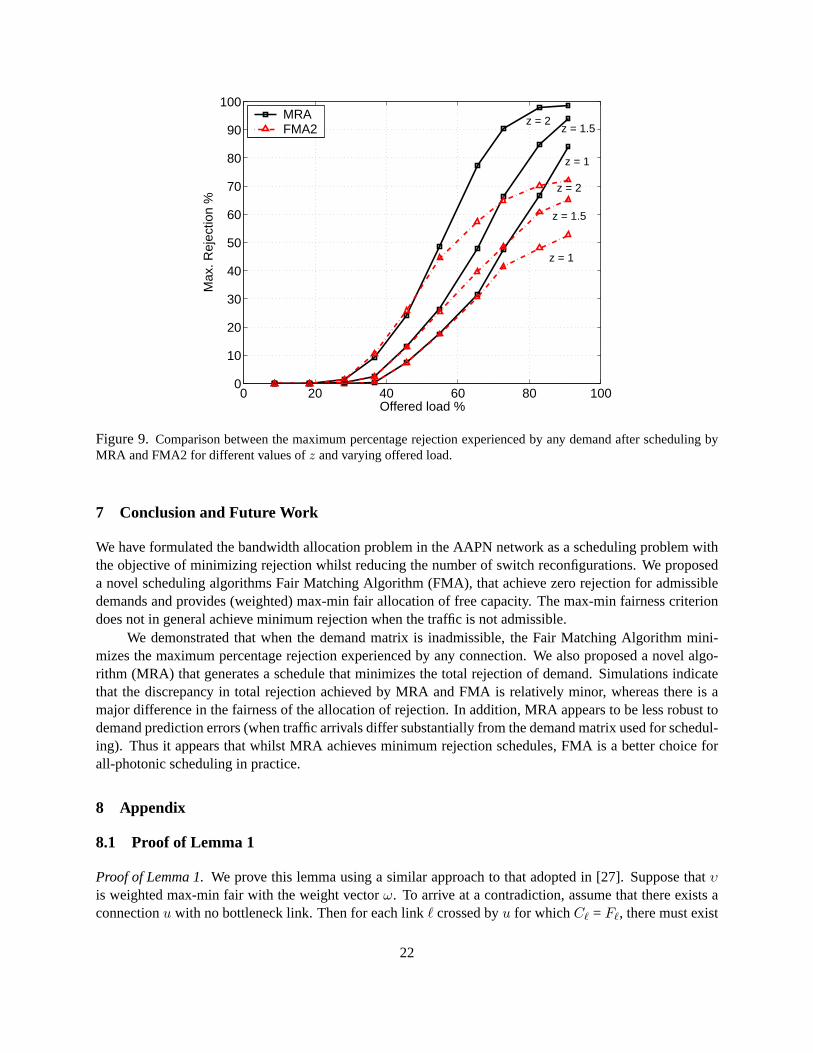
Figure8 compares the percentage of rejected demand achieved by FMA2 and MRA as the offered loadchanges for various values ofz. At high load (greater than 70%) withz = 2, there are numerous criticalelements and MRA begins to achieve less rejection than FMA2. The discrepancy is still only 2 percentat 90% load. Figure9 compares the maximum percentage rejection experienced by any demand whenscheduling is performed by FMA2 and MRA. As the offered load increases, MRA concentrates rejectionon the critical elements; the maximum percentage rejection is thus much (up to 25 percent) higher thanthat achieved by FMA2, which distributes rejection fairly amongst all competing connections. Figure10compares the average end-to-end delay experienced by packets whenscheduling is performed using FMAand MRA; the approaches yield similar average delay.

21

0 20 40 60 80 1000

10

20

30

40

50

60

70

80

90

100

Max

. Rej

ectio

n %

Offered load %

MRAFMA2

z = 1

z = 1

z = 1.5

z = 2

z = 1.5 z = 2

Figure 9. Comparison between the maximum percentage rejection experienced by any demand after scheduling byMRA and FMA2 for different values ofz and varying offered load.

7 Conclusion and Future Work

We have formulated the bandwidth allocation problem in the AAPN network as a scheduling problem withthe objective of minimizing rejection whilst reducing the number of switch reconfigurations. We proposeda novel scheduling algorithms Fair Matching Algorithm (FMA), that achieve zero rejection for admissibledemands and provides (weighted) max-min fair allocation of free capacity. The max-min fairness criteriondoes not in general achieve minimum rejection when the traffic is not admissible.

We demonstrated that when the demand matrix is inadmissible, the Fair Matching Algorithm mini-mizes the maximum percentage rejection experienced by any connection. We also proposed a novel algo-rithm (MRA) that generates a schedule that minimizes the total rejection of demand. Simulations indicatethat the discrepancy in total rejection achieved by MRA and FMA is relativelyminor, whereas there is amajor difference in the fairness of the allocation of rejection. In addition, MRA appears to be less robust todemand prediction errors (when traffic arrivals differ substantially from the demand matrix used for schedul-ing). Thus it appears that whilst MRA achieves minimum rejection schedules,FMA is a better choice forall-photonic scheduling in practice.

8 Appendix

8.1 Proof of Lemma 1

Proof of Lemma 1.We prove this lemma using a similar approach to that adopted in [27]. Suppose that υis weighted max-min fair with the weight vectorω. To arrive at a contradiction, assume that there exists aconnectionu with no bottleneck link. Then for each linkcrossed byu for whichC` = F`, there must exist

22

0 20 40 60 80 1000

0.5

1

1.5

2

2.5

3

3.5

4

Av.

Que

uein

g D

elay

(m

sec)

Offered load %

MRAFMA

Figure 10.Average queuing delay performance achieved by MRA and FMA2 for varying offered load andz = 2.

a connectionx 6= u such thatωx > ωu; thus the quantity

δ` =

{

C` − F` if F` < C`

(ωx − ωu)×Rx if F` = C`(16)

is positive. Therefore, by increasingυu by the minimumδ` over all links` crossed byu, while decreasingby the same amount the rates of the connectionsx of the links` crossed byu with F` = C`, we maintainfeasibility without decreasing the rate of any connectionk with ωk ≤ ωu; this contradicts the weightedmax-min fairness property of(υ, ω). Note thatυx −min(δ`) is always positive.

Conversely, assume that each connection has a bottleneck link with respect to the feasible set (υ, ω).Then to increase the rate of any connectionu while maintaining feasibility, we must decrease the rate of someconnectionk crossing bottleneck link of u (because we haveF` = C` by the definition of a bottlenecklink). Sinceωk ≤ ωu for all k crossing` (by the definition of a bottleneck link), the feasible set (υ, ω)satisfies the requirement for weighted max-min fairness.

8.2 Proof of Theorem 1

Proof. Consider the set of schedules that achieve minimumNs(S) = N∗s and label the schedule within this

set that achieves minimum rejectionSa. The minimum achievable rejection is no larger thanREJ(S, D, L) =max(||D||1 − L, 0), where||D||1 =

∑

i

∑

j Dij (at least one demand element must be satisfied each time-slot). ThusC(Sa) ≤ max(||D||1 − L, 0) + gN∗

s . Now consider schedules that increase the number ofswitch reconfigurations toNs(S) = N∗

s + 1 and suppose that one of these,Sb, achieves zero rejection,so thatC(Sb) = g(N∗

s + 1). The differential in costC(Sb) − C(Sa) ≥ g − max(||D||1 − L, 0). If

23

g > max(||D||1 − L, 0), then this difference is strictly positive and any schedule solvingPROBLEM 1lieswithin the set of schedules that achieve minimumNs.

In order to prove that the problem is NP-hard for this range ofg, we considerPROBLEM 2, whichfor very large values ofτ is reduced to minimizing the schedule length subject to the constraint thatNs

is minimum. Gopal et al. prove that this problem, which they refer to as the MINSWT problem, isNP -complete [11].

Suppose we had a deterministic polynomial algorithm calledsolve-G(D,L) that could solvePROBLEM1 for the identified range ofg for demand matrixD and a frame of lengthL. We could then define thealgorithm Solve-MINSWT (Algorithm 2).

Algorithm 3 Solve-MINSWTL = 1;S = solve-G(D,L);while REJ(S, D, L) > 0 do

L = L + 1;S = solve-G(D,L);

end while

Upon termination of this algorithm, the identified scheduleS is guaranteed to have the minimum num-ber of switch reconfigurations (as argued above). Since it is also the minimum length schedule that achievesREJ(S, D, L) = 0 it is also a solution toPROBLEM 2and hence the MINSWT problem. Algorithm 2 isthus a deterministic polynomial algorithm to solve the MINSWT problem. Therefore, solvingPROBLEM 1for the considered range ofg is as hard as solving MINSWT (and any other problem inNP ) and hence isNP -hard.

8.3 Proof of Theorem 2

Proof. Let u ∈ {(i, j), 1 ≤ i, j ≤ N} index the source-destination connections specified by the demandmatrix. We focus on the properties of the modified demand matrix and associatedsets at various iterationsof the while loop in Algorithm 1, so we index entities by iteration number and note that this indicates thevalue of the entity at thestart of the iteration. For example,AD(h) denotes the set of unmodified lines atthe start of iterationh of the algorithm.

We prove that FMA achieves weighted max-min fair allocation of the demands. During each iterationh of the while-loop, FMA identifies the lineγ ∈ AD(h) such thatGγ(h) = min{G`(h); ` ∈ AD(h)}. Italters the demands inaγ(h) according to (11) and after this modification, there is no subsequent modificationof these demands. Substituting (11) into the definition of the weight, we haveωu = 1 + Gγ(h) for allu ∈ aγ(h).

We demonstrate that the adjustment at iterationh leads toγ being a bottleneck link (line) foru ∈ aγ(h),i.e., after this adjustment it holds thatωz ≤ ωu for u ∈ aγ(h) andz ∈ bγ(h). Equivalently, we prove thatmin{G} is monotonically increasing with respect to the iteration number, i.e.,min{G(h)} ≤ min{G(h +1)}. The equivalence follows since theωz are obtained from adjustments prior to iterationh.

Suppose that lineβ has minimumG at iterationh + 1. Linesγ andβ have at most one connection(demand) in common. If there is no common connection, thenGβ(h + 1) = Gβ(h) ≥ Gγ(h). If there is a

24

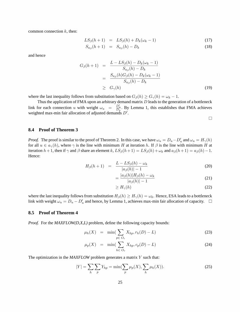
common connectionk, then:

LSβ(h + 1) = LSβ(h) + Dk(ωk − 1) (17)

Saβ(h + 1) = Saβ

(h)−Dk (18)

and hence

Gβ(h + 1) =L− LSβ(h)−Dk(ωk − 1)

Saβ(h)−Dk

=Saβ

(h)Gβ(h)−Dk(ωk − 1)

Saβ(h)−Dk

≥ Gγ(h) (19)

where the last inequality follows from substitution based onGβ(h) ≥ Gγ(h) = ωk − 1.Thus the application of FMA upon an arbitrary demand matrixD leads to the generation of a bottleneck

link for each connectionu with weight ωu = D′

u

Du. By Lemma 1, this establishes that FMA achieves

weighted max-min fair allocation of adjusted demandsD′.

8.4 Proof of Theorem 3

Proof. The proof is similar to the proof of Theorem 2. In this case, we haveωu = Du−D′u andωu = Hγ(h)

for all u ∈ aγ(h), whereγ is the line with minimumH at iterationh. If β is the line with minimumH atiterationh+1, then ifγ andβ share an elementk, LSβ(h+1) = LSβ(h)+ωk andaβ(h+1) = aβ(h)−1.Hence:

Hβ(h + 1) =L− LSβ(h)− ωk

|aβ(h)| − 1(20)

=|aβ(h)|Hβ(h)− ωk

|aβ(h)| − 1(21)

≥ Hγ(h) (22)

where the last inequality follows from substitutionHβ(h) ≥ Hγ(h) = ωk. Hence, ESA leads to a bottlenecklink with weightωu = Du−D′

u and hence, by Lemma 1, achieves max-min fair allocation of capacity.

8.5 Proof of Theorem 4

Proof. For theMAXFLOW(D,X,L)problem, define the following capacity bounds:

µh(X) = min(∑

p∈ Oc

Xhp, rh(D)− L) (23)

µp(X) = min(∑

h∈ Or

Xhp, cp(D)− L) (24)

The optimization in theMAXFLOWproblem generates a matrixY such that:

|Y | =∑

h

∑

p

Yhp = min(∑

p

µp(X),∑

h

µh(X)). (25)

25

This is an application of the max-flow min-cut theorem [36] (see Figure4).Consider an arbitrary rejection matrixDw and setB =MAXFLOW(D, Dw, L). Then we can write

Dw = B + Q whereQ is a non-negative matrix. Now consider the conditions necessary forDw to achieveminimum rejection. First,Dw

hp = 0 if h /∈ Or andp /∈ Oc (any non-zero values constitute unnecessaryrejection).

Without loss of generality, suppose that∑

p µp(Dw) <

∑

h µh(Dw). Then for each rowh ∈ Or,∑

p Bhp = µp(Dw). This implies that rowh either achieves its required rejection solely fromB (i.e.,

rh(B) = rh(D) − L), or thatBhp = Dwhp for all p ∈ Oc. In the latter case,Dw must contain additional

rejection (positive entries) on rowh at thenon-critical connections. If Dw is to achieve minimum totalrejection,rh(Q) = rh(D)− L− rh(B).

Now consider the columns ofDw. After the generation ofB, the rejection on columnp is cp(B). Thenfor minimum rejection we require thatcp(Q) = cp(D) − L − cp(B). Note that ifrh(B) does not satisfythe rejection requirements of rowh, thenQhp = 0. Thus, no positive elements ofQ contribute to requiredrejection on both a rowh and a columnp.

Based on this discussion, ifDw achieves minimum rejection, we can express its rejection|Dw| as:

|Dw| =∑

h

∑

p

(B + Q)

= |B|+∑

h∈Or

(rh(D)− L− rh(B))

+∑

p∈Oc

(cp(D)− L− cp(B))

=∑

h∈Or

(rh(D)− L) +∑

p∈Oc

(cp(D)− L)− |B| (26)

Therefore, in order forDw to achieve minimum rejection,|B| must be maximized (the first twoterms are functions solely ofD andL). Compare the solutionsB = MAXFLOW(D, Dw, L) andA =MAXFLOW(D, D, L). SinceDw

hp ≤ Dhp for any (h, p), the constraints in the second problem are looser,which implies that|A| ≥ |B|, irrespective of the particular values inDw. Note thatA is also a solution toMAXFLOW(D, A, L).

Hence if we ensure thatDwhp ≥ Ahp for all (h, p), we derive|B| = |A|, which implies that|B| attains

its maximum value (and hence|Dw| is the minimum rejection). We can thus construct a rejection matrixthat achieves minimum rejection by solving A =MAXFLOW(D, D, L), and settingD

′′

= A + Q, whereQsatisfies the constraints specified in the theorem. If a scheduleS decomposes the demand into an allocatedmatrixD′ and this rejection matrixD

′′

, then it achieves minimum rejection.

References

[1] L. Xu, H.G. Perros, and G. Rouskas, “Techniques for optical packet switching and optical burstswitching,” IEEE Comm. Mag., vol. 39, no. 1, pp. 136–142, Jan. 2001.

[2] R. Ramaswami and K.N. Sivarajan, “Routing and wavelength assignment in all-optical networks,”IEEE/ACM Trans. Networking, vol. 3, no. 5, pp. 489–500, Oct. 1995.

[3] G.V. Bochmann, M.J. Coates, T. Hall, L.G. Mason, R. Vickers, and O.Yang, “The agile all-photonicnetwork: An architectural outline,” inProc. Queens’ Biennial Symp. Comms., Kingston, Canada, June2004.

26

[4] L.G. Mason, A. Vinokurov, N. Zhao, and D. Plant, “Topological design and dimensioning of agile allphotonic networks,”Computer Networks, vol. 50, no. 2, pp. 268–287, Feb. 2006.

[5] I. Keslassy, M. Kodialam, T.V. Lakshman, and D. Stiliadis, “Schedulingschemes for delay graphswith applications to optical packet networks,” inProc. IEEE Work. High Perf. Switch. and Routing,Phoenix, AZ, Apr. 2003.

[6] X. Liu, N. Saberi, M.J. Coates, and L.G. Mason, “A comparison between time-slot scheduling ap-proaches for all-photonic networks,” inInt. Conf. on Inf., Comm. and Sig. Proc (ICICS), Bangkok,Thailand, Dec. 2005.

[7] N. Saberi and M.J. Coates, “Bandwidth reservation in optical WDM/TDM star networks,” inProc.Queens’ Biennial Symp. Comms., Kingston, Canada, June 2004.

[8] A. Ganz and Y. Gao, “A time-wavelength assignment algorithm for a WDMstar network,” inProc.IEEE Infocom, Florence, Italy, 1992.

[9] A.Ganz and Y.Gao, “Efficient algorithms for SS/TDMA scheduling,”IEEE Trans. Comm., vol. 40,pp. 1367–1374, August 1992.

[10] C. A. Pomalaza-Raez, “A note on efficient SS/TDMA assignment algorithms,” IEEE Trans. Comm.,vol. 36, pp. 1078–1082, 1988.

[11] I. S. Gopal and C. K. Wong, “Minimizing the number of switchings in an SS/TDMA system,” IEEETrans. Comm., vol. 33, pp. 1497–1501, June 1985.

[12] B. Towles and W. J. Dally, “Guaranteed scheduling for switches withconfiguration overhead,”IEEE/ACM Trans. Networking, vol. 11, pp. 835–847, October 2003.

[13] T. Gonzalez and S. Sahni, “Open shop scheduling to minimize finish time,”J. ACM, vol. 23, pp.665–679, Oct. 1976.

[14] P. Crescenzi, X. Deng, and C. H. Papadimitriou, “On approximating ascheduling problem,”J. Com-binatorial Optimization, vol. 5, pp. 287–297, 2001.

[15] G. Bongiovanni, D. Coppersmith, and C.K. Wong, “An optimal time slot assignment algorithm for anSS/TDMA system with variable number of transponders,”IEEE Trans. Comm., vol. 29, pp. 721–726,Oct. 1981.

[16] I.S. Gopal, G. Bongiovanni, M. A. Bonuccelli, D. T. Tang, and C. K. Wang, “An optimal switchingalgorithm for multibeam satellite systems with variable bandwidth beams,”IEEE Trans. Comm., vol.30, pp. 2475–2481, Nov. 1982.

[17] T. Inukai, “An efficient SS/TDMA time slot assignment algorithm,”IEEE Trans. Comm., vol. 27, pp.1449–1455, May 1979.

[18] R. L. Graham, “Bounds on multiprocessing timing anomalies,”SIAM J. Applied Mathematics, vol.17, pp. 416–429, March 1969.

[19] R. L. Graham, E. L. Lawler, J. K. Lenstra, and K. Rinnooy Kan, “Optimization and approximation indeterministic scheduling: A survey,”Ann. Disc. Math., pp. 287–326, 1979.

27

[20] D. McLaughlin, S. Sardesai, and P. Dasgupta, “Preemptive scheduling for distributed systems,” inProc.11th Int. Conf. Parallel and Distributed Computing Systems, Chicago, Illinois USA, Sept. 1998.

[21] K. Jansen and M.I. Sviridenko, “Polynomial time approximation schemesfor the multiprocessor openand flow shop scheduling problem,” in27th International Colloquium on Automata, Languages andProgramming, Geneva, Switzerland, July 2000, pp. 878–889.

[22] K. Jansen, R. Solis-Oba, and M.I. Sviridenko, “A linear time approximation scheme for the job shopscheduling problem,” inProc. Third Inter. Workshop Approximation Algorithms for CombinatorialOptimization Problems, Aug. 1999, pp. 177–188.

[23] C.H. Papadimitriou and K. Steiglitz, Combinatorial optimization: algorithms and complexity,Prentice-Hall, 1982.

[24] S. Micali and V. V. Vazirani, “AnO(√

‖V ‖‖E‖) algorithm for finding maximum matching in generalgraphs,” inProc. IEEE Symp. on Found. Comp. Sci., Syracuse, NY, 1980, pp. 17–27.

[25] R.M. Karp, “Reducibility among combinatorial problems,” inProc. Complexity of computer compu-tations, R.E. Miller and J.W. Thatcher, Eds., New York, NY, 1972, pp. 85–103,Plenum Press.

[26] Ed. D. Hochbaum,Approximation Algorithms for NP-Hard Problems, PWS Publishing Company,Boston, MA, 1996.

[27] D. Bertsekas and R. Gallager,Data Networks, Prentice Hall, Englewood Cliffs, NJ, 1992.

[28] P. Marbach, “Priority service and max-min fairness,”IEEE/ACM Trans. Networking, pp. 733–746,Oct. 2003.

[29] A. Charny, D. Clark, and R. Jain, “Congestion control with explicitrate indication,” inProc. ICC,Seattle, WA, Jun. 1995.

[30] M.A. Marsan, A. Bianco, E. Leonardi, F. Neri, and A. Nucci, “Simple on-line scheduling algorithmsfor all-optical broadcast-and select networks,”IEEE European Trans. Telecom., vol. 11, no. 1, pp.109–116, Jan. 2000.

[31] L. R. Ford, Jr., and D. R. Fulkerson, “Maximal flow through a network,” Canadian. J. Math., pp.399–404, 1956.

[32] J. Edmonds and R. M. Karp, “Theoretical improvements in algorithmic efficiency for network flowproblems,”J. Assoc. Comput. Mach., pp. 248–264, 1972.

[33] “OPNET modeler 10.5,” http://www.opnet.com.

[34] “Passive measurement and analysis (PMA) project,” http://pma.nlanr.net/Traces/Traces/daily.

[35] T. Ahmed and M.J. Coates, “Predicting flow vectors,” Tech. Rep., McGill University, Mon-treal, Canada, Sept. 2005, available athttp://www.tsp.ece.mcgill.ca/Networks/publications.html.

[36] P. Elias, A. Feinstein, and C. E. Shannon, “Note on maximum flow through a network,”IRE Transac-tions on Information Theory IT-2, pp. 117–119, 1956.

28