Parallel ½-approx Weighted Matching Algorithm

A Parallel ½-approx Weighted Matching Algorithm

Mahantesh Halappanavar, Florin Dobrian and

Alex Pothen

CSCAPES Seminar. 16 September, 2008.

1

Outline

1. Introduction

2. Brief Survey of Parallel Matching Algorithms

3. A ½-approx Parallel Matching Algorithm

4. Computational Results

5. Conclusions and Future work

2

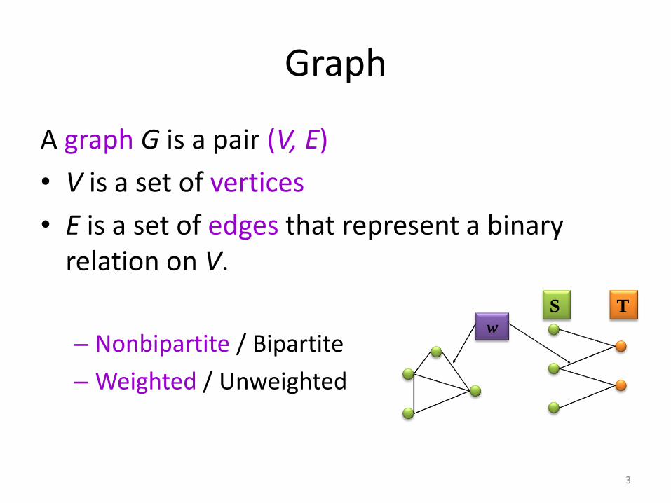
Graph

A graph G is a pair (V, E)

• V is a set of vertices

• E is a set of edges that represent a binary relation on V.

– Nonbipartite / Bipartite

– Weighted / Unweighted

w

S T

3

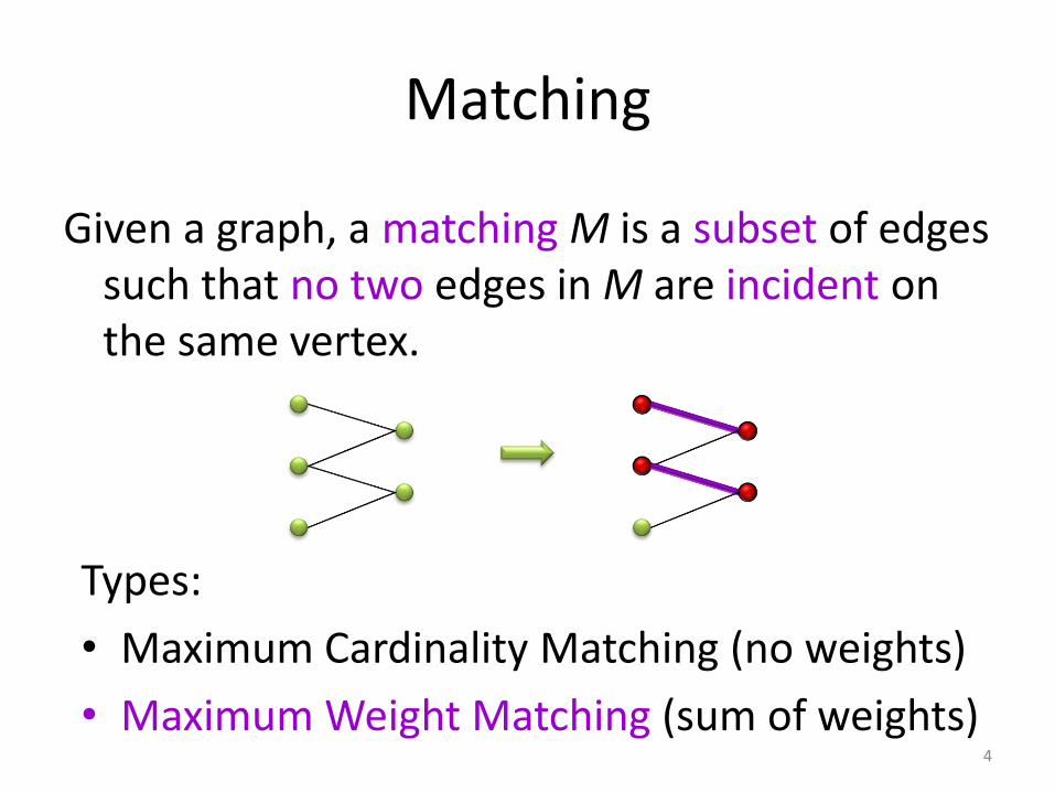
Matching

Given a graph, a matching M is a subset of edges such that no two edges in M are incident on the same vertex.

Types:

• Maximum Cardinality Matching (no weights)

• Maximum Weight Matching (sum of weights)4

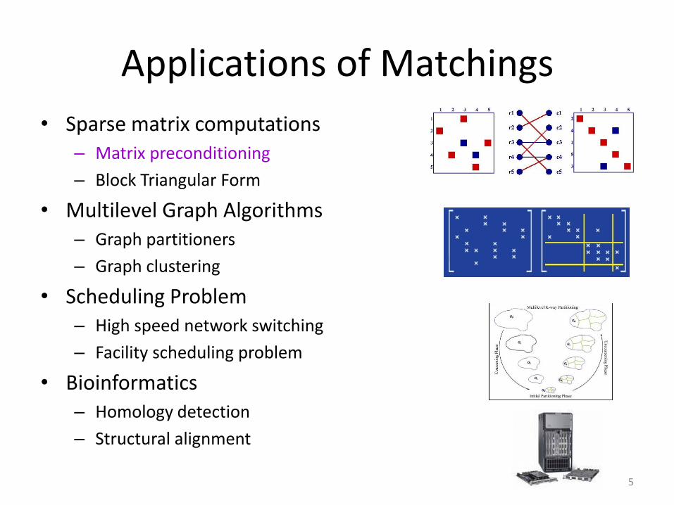
Applications of Matchings

• Sparse matrix computations– Matrix preconditioning

– Block Triangular Form

• Multilevel Graph Algorithms– Graph partitioners

– Graph clustering

• Scheduling Problem– High speed network switching

– Facility scheduling problem

• Bioinformatics– Homology detection

– Structural alignment

5

Outline

1. Introduction





6

A Brief Survey of Parallel Matching Algorithms

• Bipartite Graphs:

– Auction-based algorithms

– Augmentation-based algorithms

• Nonbipartite Graphs:

– Augmentation-based algorithms

Note: Non-exhaustive survey7

Auction-based Algorithms

• Primary work: – Dimitri P. Bertsekas, MIT

• Basic idea:– Buyers bid for objects

– Iterative process

– Two basic approaches:• Gauss-Seidel: one buyer at a time

• Jacobi: all buyers bid concurrently

– Reverse auctions for asymmetric problems

– Combined forward/reverse (hybrid) approaches for performance

8

Auction-based Algorithms

• Parallel work:– 1979: Bertsekas

– 1989: Bertsekas and Castanon

– 1989: Kempka, Kennington and Zaki (Alliant FX/8)

– 1990: Wein and Zenios : (Connection Machine, CM2)

– 1992: Goldberg, Plotkin, Shmoys and Tardos (interior point methods)

– 2003: Reidy and Demmel (In the context of sparse direct solvers – SuperLU)

9

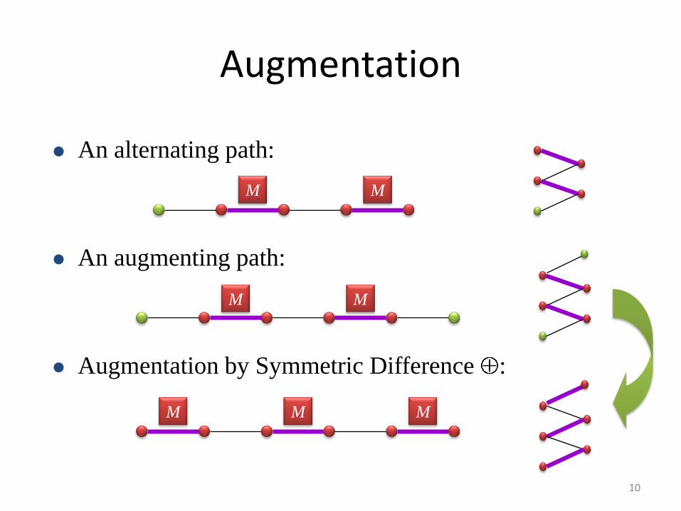
Augmentation

M M

MM

MMM

An alternating path:

An augmenting path:

Augmentation by Symmetric Difference :

10

Augmentation-based algorithms

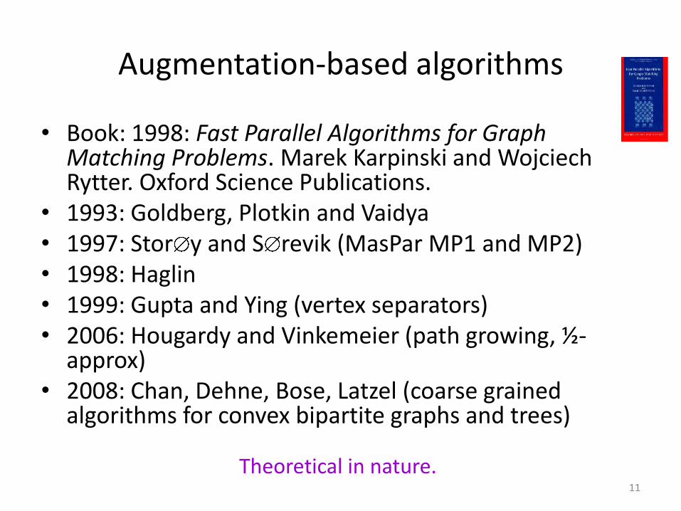
• Book: 1998: Fast Parallel Algorithms for Graph Matching Problems. Marek Karpinski and WojciechRytter. Oxford Science Publications.

• 1993: Goldberg, Plotkin and Vaidya• 1997: Stor y and S revik (MasPar MP1 and MP2)• 1998: Haglin• 1999: Gupta and Ying (vertex separators)• 2006: Hougardy and Vinkemeier (path growing, ½-

approx)• 2008: Chan, Dehne, Bose, Latzel (coarse grained

algorithms for convex bipartite graphs and trees)

Theoretical in nature.11

Outline

1. Introduction



– Introduction

– Implementation Details



12

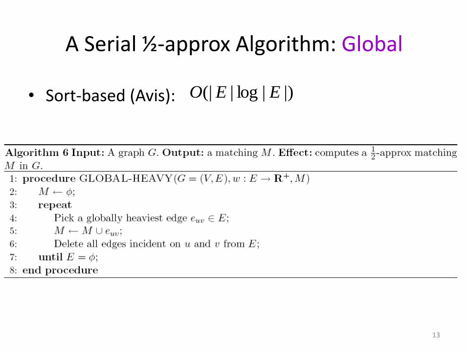
A Serial ½-approx Algorithm: Global

• Sort-based (Avis): |)|log|(| EEO

13

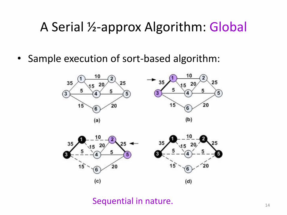
A Serial ½-approx Algorithm: Global

• Sample execution of sort-based algorithm:

Sequential in nature.14

A Serial ½-approx Algorithm: Local

• Robert Preis’s LAM algorithm: O(|E|)

15

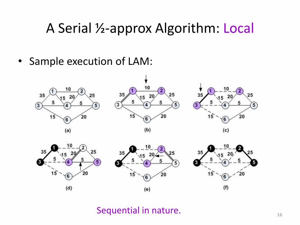
A Serial ½-approx Algorithm: Local

• Sample execution of LAM:

Sequential in nature.16

Assumptions for Parallelization

• Vertex-oriented data structures for graph representation

• Graph distributed among processors via vertex partitioning

• Owner-computes Model: each processor owns a set of vertices that it is responsible for

17

Towards Parallelization

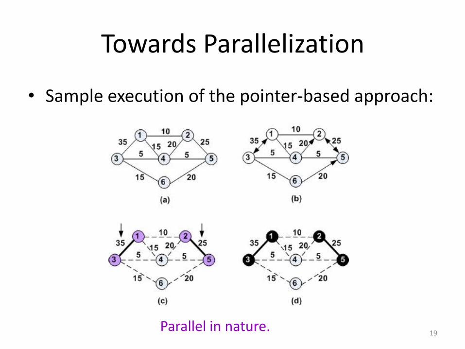
Pointer-based algorithm:

1. For each vertex, set a pointer to the heaviest adjacent vertex.

2. If two vertices point to each other, then add these (locally dominating) edges to the matching.

3. Remove all edges incident on the matched edges, reset the pointers, and repeat.

18

Towards Parallelization

• Sample execution of the pointer-based approach:

Parallel in nature.19

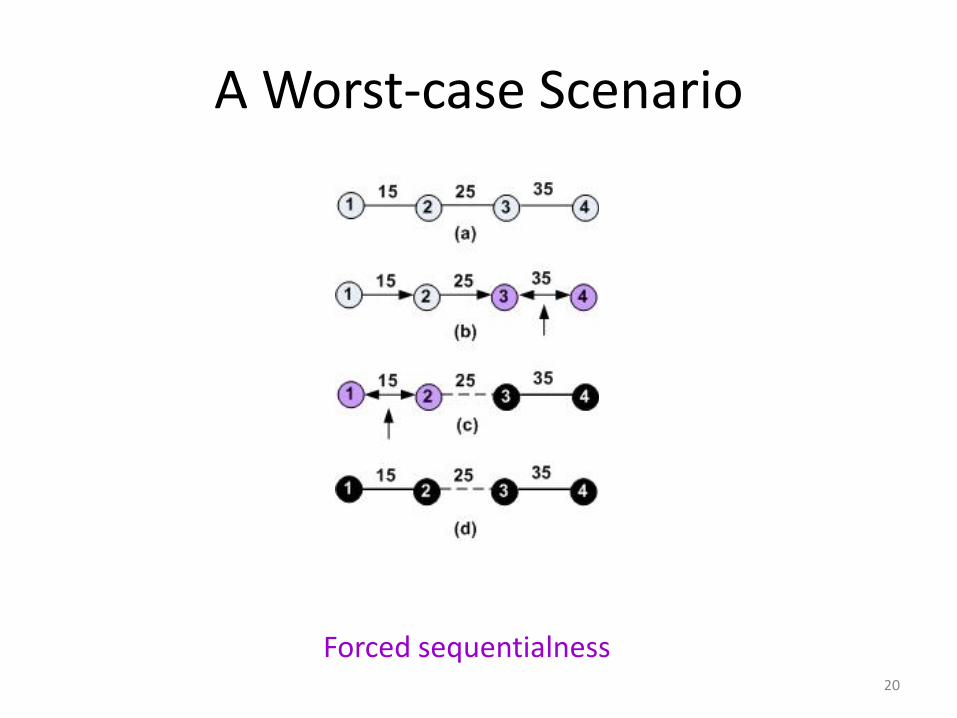
A Worst-case Scenario

Forced sequentialness20

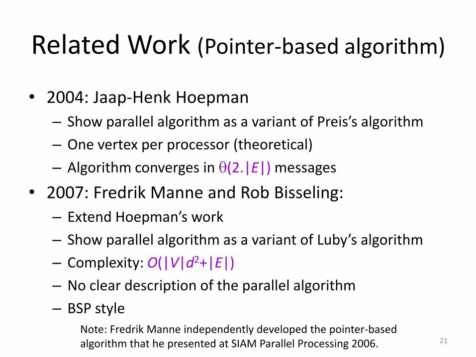
Related Work (Pointer-based algorithm)

• 2004: Jaap-Henk Hoepman

– Show parallel algorithm as a variant of Preis’s algorithm

– One vertex per processor (theoretical)

– Algorithm converges in (2.|E|) messages

• 2007: Fredrik Manne and Rob Bisseling:

– Extend Hoepman’s work

– Show parallel algorithm as a variant of Luby’s algorithm

– Complexity: O(|V|d2+|E|)

– No clear description of the parallel algorithm

– BSP styleNote: Fredrik Manne independently developed the pointer-based algorithm that he presented at SIAM Parallel Processing 2006. 21

Outline

1. Introduction



– Introduction

– Implementation Details



22

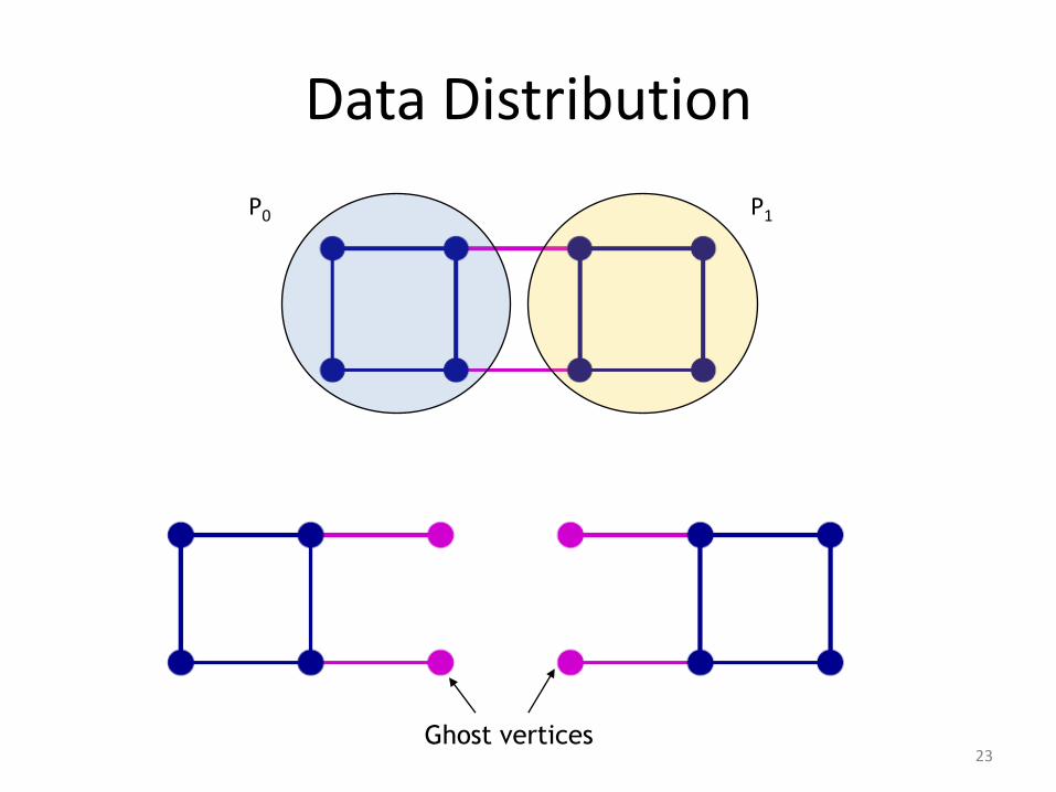
Data Distribution

P0 P1

Ghost vertices23

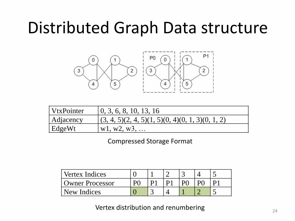
Distributed Graph Data structure

VtxPointer 0, 3, 6, 8, 10, 13, 16

Adjacency (3, 4, 5)(2, 4, 5)(1, 5)(0, 4)(0, 1, 3)(0, 1, 2)

EdgeWt w1, w2, w3, …

Vertex Indices 0 1 2 3 4 5

Owner Processor P0 P1 P1 P0 P0 P1

New Indices 0 3 4 1 2 5

Compressed Storage Format

Vertex distribution and renumbering24

Distributed Graph Data structure

Processor 0: Processor Pointer 0, 3, 6

VtxPointer 0, 3, 5, 8

Adjacency (m) (1, 2, 5)(0, 2)(0, 1, 3)

EdgeWt e1, e2, e3, …

VtxWt v1, v2, v3, …

Processor 1: Processor Pointer 0, 3, 6

VtxPointer 0, 3, 5, 8

Adjacency (2, 4, 5)(3, 5)(0, 3, 4)

EdgeWt e1, e2, e3, …

VtxWt v1, v2, v3, …

Data structure on each processor

FindOwner(ghost-vtx): O(lg P); Storage: O(P) 25

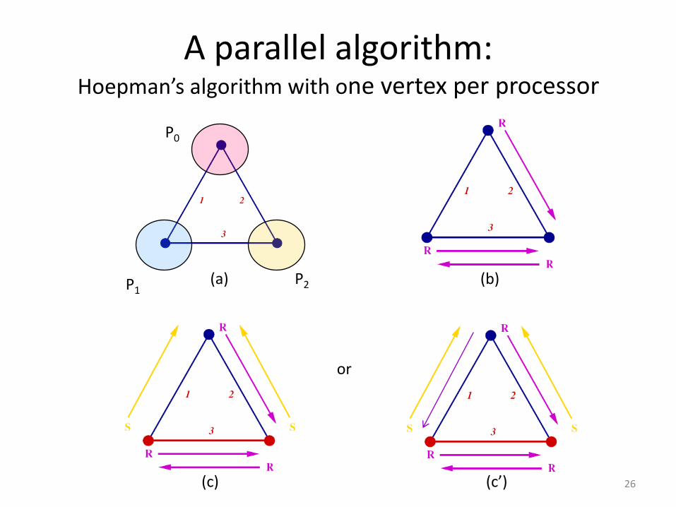
A parallel algorithm: Hoepman’s algorithm with one vertex per processor

(b)

(c)

(a)

P0

P2P1

(c’)

or

26

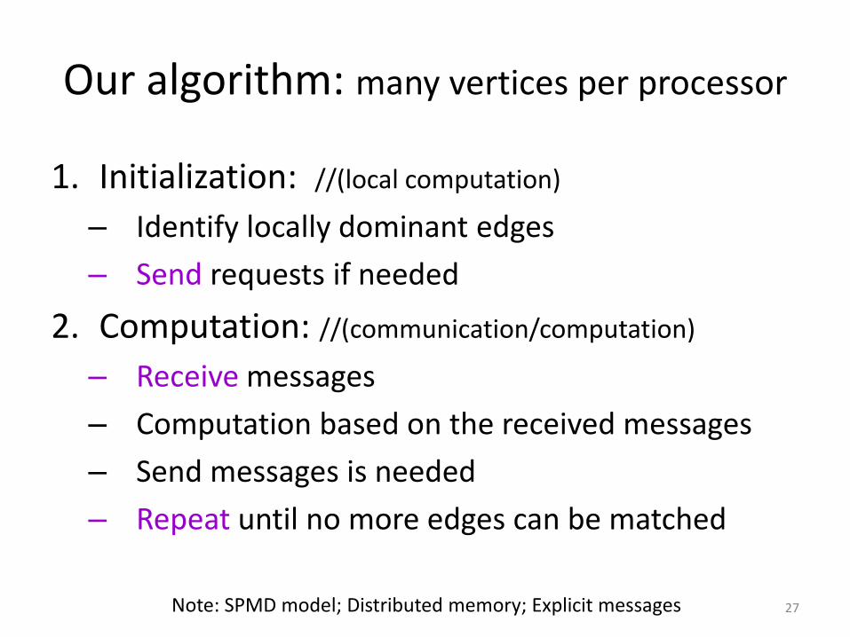
Our algorithm: many vertices per processor

1. Initialization: //(local computation)

– Identify locally dominant edges

– Send requests if needed

2. Computation: //(communication/computation)

– Receive messages

– Computation based on the received messages

– Send messages is needed

– Repeat until no more edges can be matched

Note: SPMD model; Distributed memory; Explicit messages 27

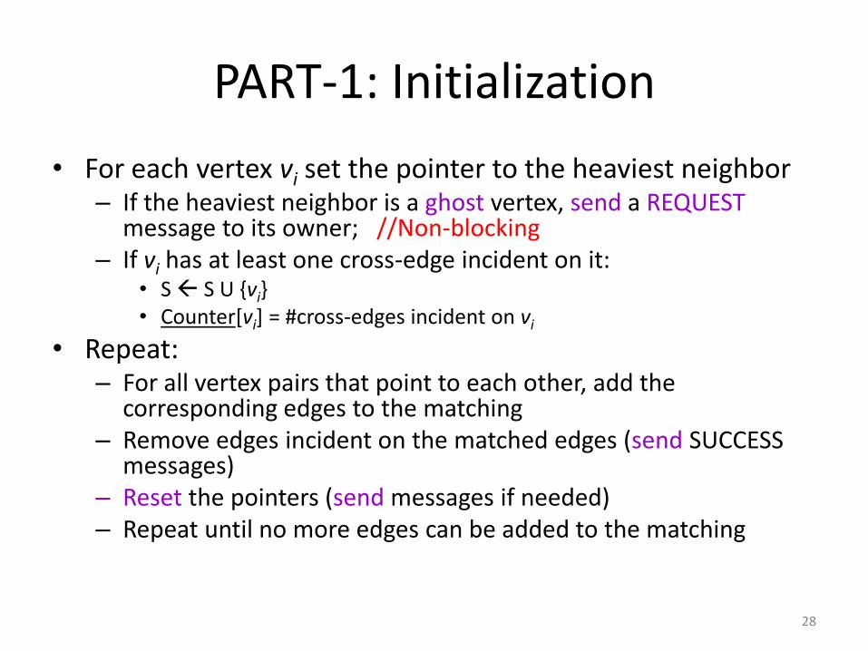
PART-1: Initialization

• For each vertex vi set the pointer to the heaviest neighbor– If the heaviest neighbor is a ghost vertex, send a REQUEST

message to its owner; //Non-blocking– If vi has at least one cross-edge incident on it:

• S S U {vi} • Counter[vi] = #cross-edges incident on vi

• Repeat: – For all vertex pairs that point to each other, add the

corresponding edges to the matching– Remove edges incident on the matched edges (send SUCCESS

messages)– Reset the pointers (send messages if needed)– Repeat until no more edges can be added to the matching

28

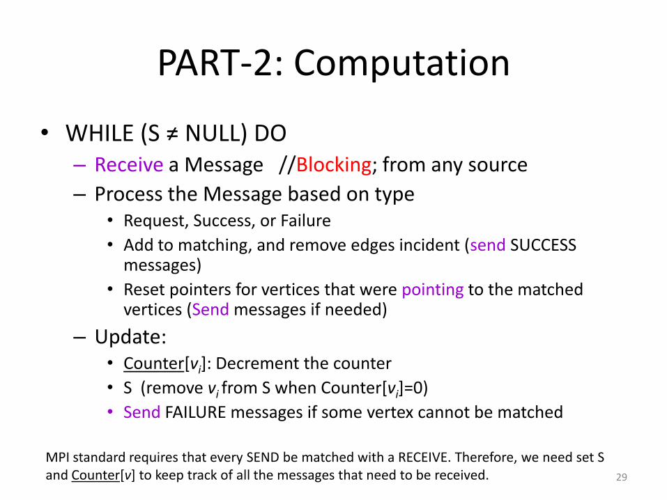
PART-2: Computation

• WHILE (S ≠ NULL) DO– Receive a Message //Blocking; from any source

– Process the Message based on type• Request, Success, or Failure

• Add to matching, and remove edges incident (send SUCCESS messages)

• Reset pointers for vertices that were pointing to the matched vertices (Send messages if needed)

– Update:• Counter[vi]: Decrement the counter

• S (remove vi from S when Counter[vi]=0)

• Send FAILURE messages if some vertex cannot be matched

MPI standard requires that every SEND be matched with a RECEIVE. Therefore, we need set S and Counter[v] to keep track of all the messages that need to be received. 29

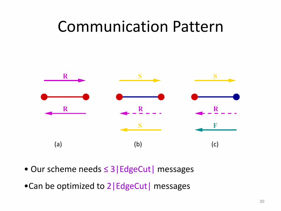
Communication Pattern

(a) (b) (c)

• Our scheme needs ≤ 3|EdgeCut| messages

•Can be optimized to 2|EdgeCut| messages

30

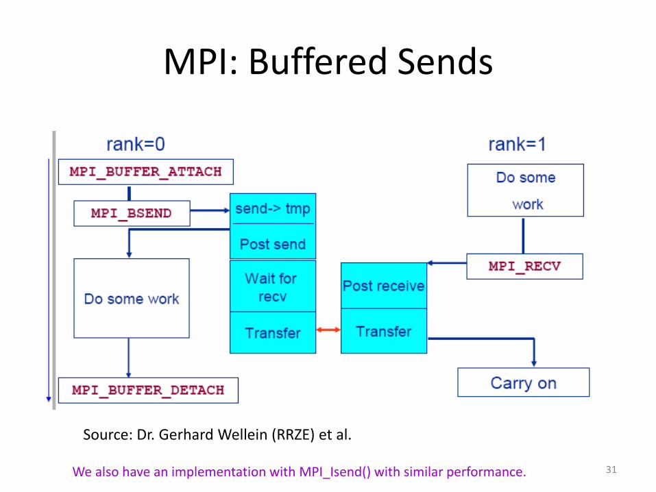
MPI: Buffered Sends

Source: Dr. Gerhard Wellein (RRZE) et al.

We also have an implementation with MPI_Isend() with similar performance. 31

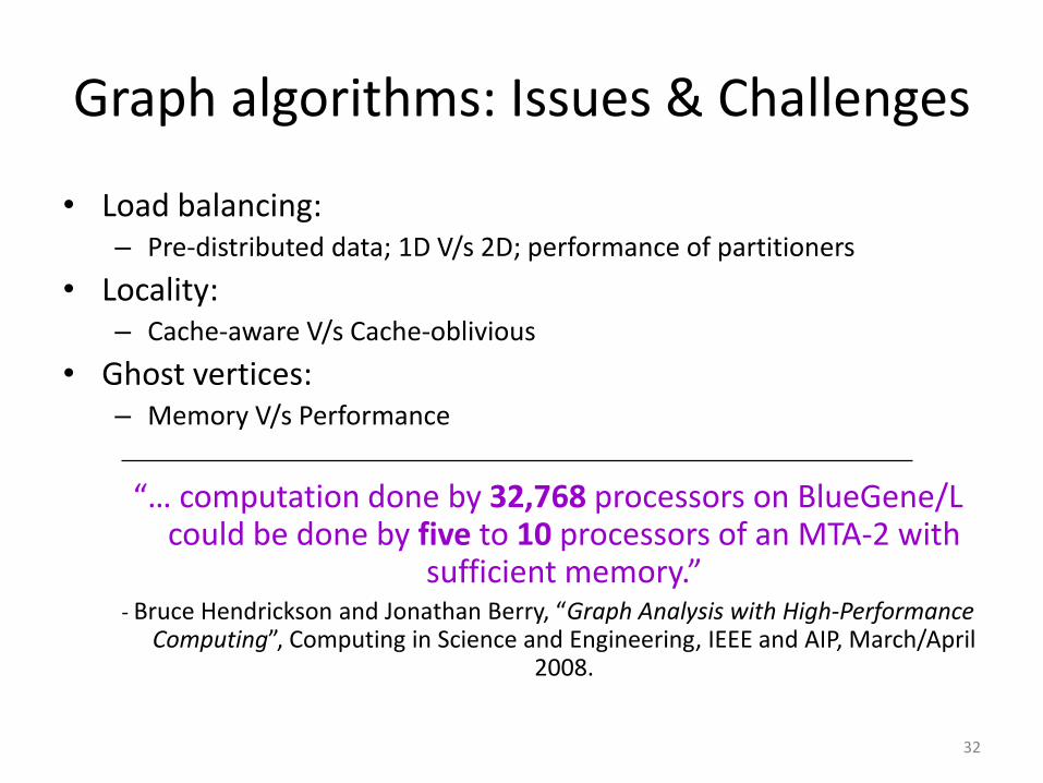
Graph algorithms: Issues & Challenges

• Load balancing:– Pre-distributed data; 1D V/s 2D; performance of partitioners

• Locality:– Cache-aware V/s Cache-oblivious

• Ghost vertices:– Memory V/s Performance

“… computation done by 32,768 processors on BlueGene/L could be done by five to 10 processors of an MTA-2 with

sufficient memory.”- Bruce Hendrickson and Jonathan Berry, “Graph Analysis with High-Performance

Computing”, Computing in Science and Engineering, IEEE and AIP, March/April 2008.

32

Outline

1. Introduction




– Performance of serial ½-approx algorithm

– Performance of parallel ½-approx algorithm


33

Platform Details

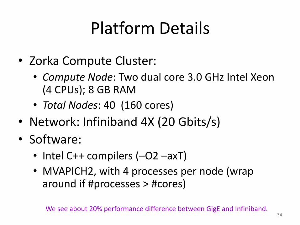
• Zorka Compute Cluster:• Compute Node: Two dual core 3.0 GHz Intel Xeon

(4 CPUs); 8 GB RAM

• Total Nodes: 40 (160 cores)

• Network: Infiniband 4X (20 Gbits/s)

• Software:• Intel C++ compilers (–O2 –axT)

• MVAPICH2, with 4 processes per node (wrap around if #processes > #cores)

We see about 20% performance difference between GigE and Infiniband.34

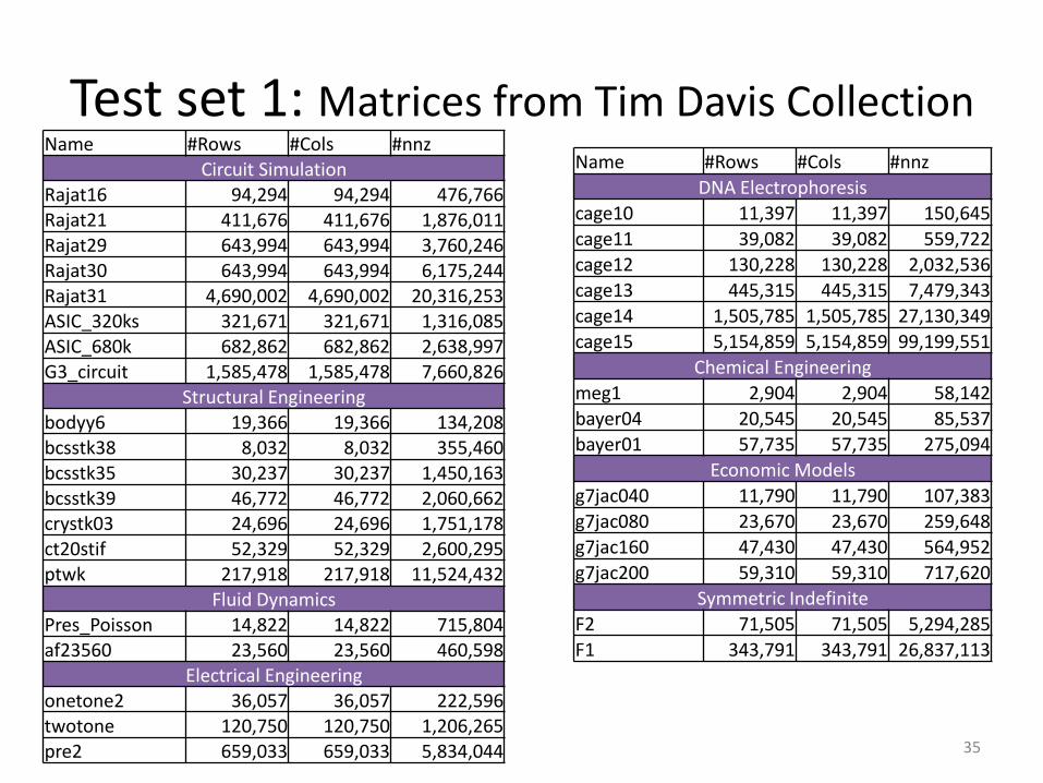
Test set 1: Matrices from Tim Davis CollectionName #Rows #Cols #nnz

Circuit SimulationRajat16 94,294 94,294 476,766Rajat21 411,676 411,676 1,876,011Rajat29 643,994 643,994 3,760,246Rajat30 643,994 643,994 6,175,244Rajat31 4,690,002 4,690,002 20,316,253ASIC_320ks 321,671 321,671 1,316,085ASIC_680k 682,862 682,862 2,638,997G3_circuit 1,585,478 1,585,478 7,660,826

Structural Engineeringbodyy6 19,366 19,366 134,208bcsstk38 8,032 8,032 355,460bcsstk35 30,237 30,237 1,450,163bcsstk39 46,772 46,772 2,060,662crystk03 24,696 24,696 1,751,178ct20stif 52,329 52,329 2,600,295ptwk 217,918 217,918 11,524,432

Fluid DynamicsPres_Poisson 14,822 14,822 715,804af23560 23,560 23,560 460,598

Electrical Engineeringonetone2 36,057 36,057 222,596twotone 120,750 120,750 1,206,265pre2 659,033 659,033 5,834,044

Name #Rows #Cols #nnz

DNA Electrophoresis

cage10 11,397 11,397 150,645

cage11 39,082 39,082 559,722

cage12 130,228 130,228 2,032,536

cage13 445,315 445,315 7,479,343

cage14 1,505,785 1,505,785 27,130,349

cage15 5,154,859 5,154,859 99,199,551

Chemical Engineering

meg1 2,904 2,904 58,142

bayer04 20,545 20,545 85,537

bayer01 57,735 57,735 275,094

Economic Models

g7jac040 11,790 11,790 107,383

g7jac080 23,670 23,670 259,648

g7jac160 47,430 47,430 564,952

g7jac200 59,310 59,310 717,620

Symmetric Indefinite

F2 71,505 71,505 5,294,285

F1 343,791 343,791 26,837,113

35

Performance of Sequential Algorithm

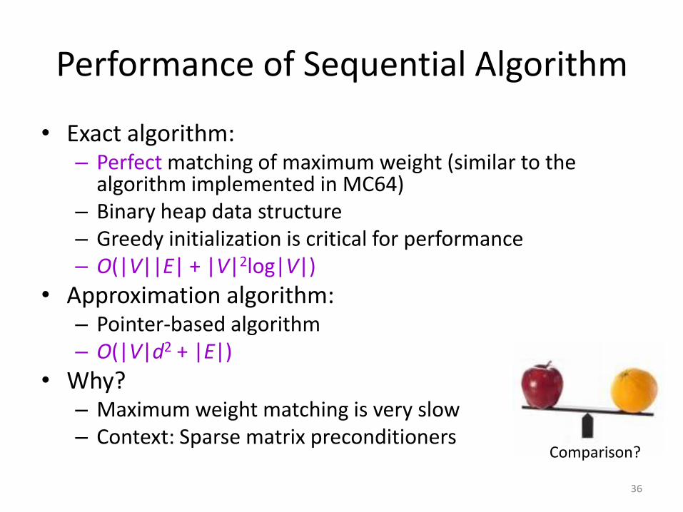
• Exact algorithm:– Perfect matching of maximum weight (similar to the

algorithm implemented in MC64)– Binary heap data structure– Greedy initialization is critical for performance– O(|V||E| + |V|2log|V|)

• Approximation algorithm:– Pointer-based algorithm– O(|V|d2 + |E|)

• Why?– Maximum weight matching is very slow– Context: Sparse matrix preconditioners

Comparison?

36

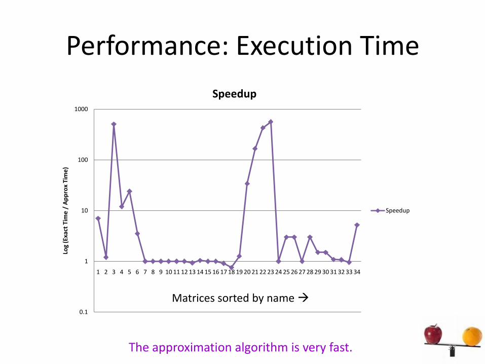
Performance: Execution Time

0.1

1

10

100

1000

1 2 3 4 5 6 7 8 9 10 11 12 13 14 15 16 17 18 19 20 21 22 23 24 25 26 27 28 29 30 31 32 33 34

Log

(Exa

ct T

ime

/ A

pp

rox

Tim

e)

Speedup

Speedup

Matrices sorted by name

The approximation algorithm is very fast. 37

Outline

1. Introduction




– Performance of serial ½-approx algorithm

– Performance of parallel ½-approx algorithm


38

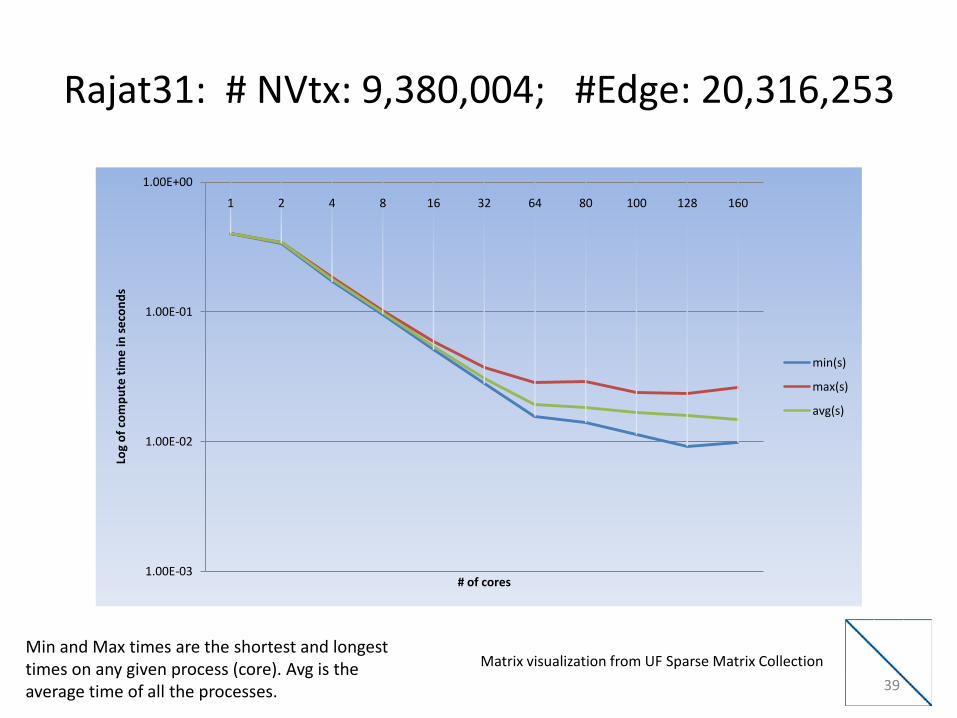
Rajat31: # NVtx: 9,380,004; #Edge: 20,316,253

1.00E-03

1.00E-02

1.00E-01

1.00E+00

1 2 4 8 16 32 64 80 100 128 160

Log

of

com

pu

te t

ime

in s

eco

nd

s

# of cores

min(s)

max(s)

avg(s)

Matrix visualization from UF Sparse Matrix CollectionMin and Max times are the shortest and longest times on any given process (core). Avg is the average time of all the processes. 39

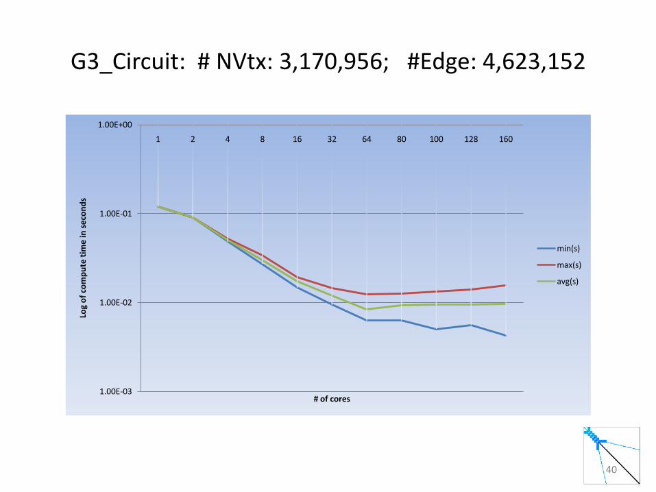
G3_Circuit: # NVtx: 3,170,956; #Edge: 4,623,152

1.00E-03

1.00E-02

1.00E-01

1.00E+00

1 2 4 8 16 32 64 80 100 128 160

Log

of

com

pu

te t

ime

in s

eco

nd

s

# of cores

min(s)

max(s)

avg(s)

40

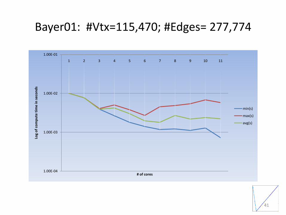
Bayer01: #Vtx=115,470; #Edges= 277,774

1.00E-04

1.00E-03

1.00E-02

1.00E-01

1 2 3 4 5 6 7 8 9 10 11

Log

of

com

pu

te t

ime

in s

eco

nd

s

# of cores

min(s)

max(s)

avg(s)

41

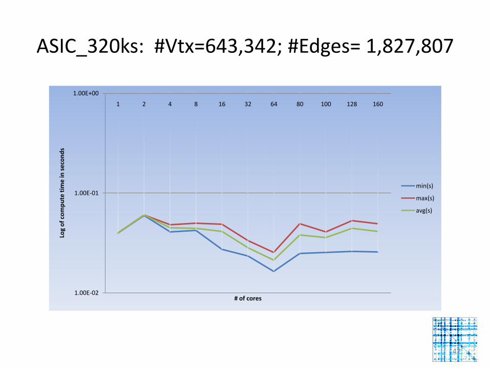
ASIC_320ks: #Vtx=643,342; #Edges= 1,827,807

1.00E-02

1.00E-01

1.00E+00

1 2 4 8 16 32 64 80 100 128 160

Log

of

com

pu

te t

ime

in s

eco

nd

s

# of cores

min(s)

max(s)

avg(s)

42

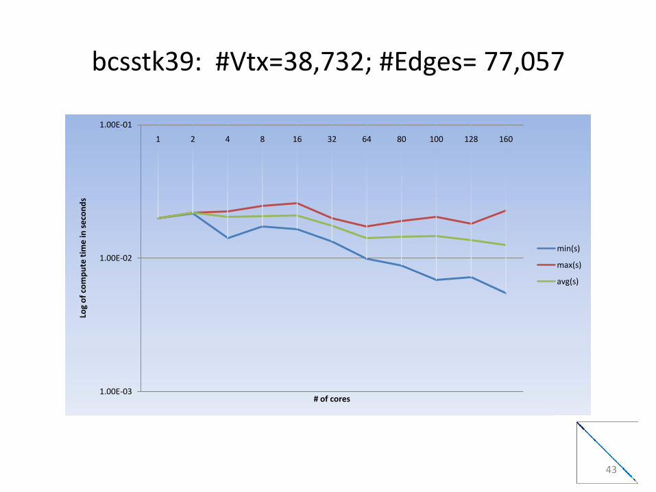
bcsstk39: #Vtx=38,732; #Edges= 77,057

1.00E-03

1.00E-02

1.00E-01

1 2 4 8 16 32 64 80 100 128 160

Log

of

com

pu

te t

ime

in s

eco

nd

s

# of cores

min(s)

max(s)

avg(s)

43

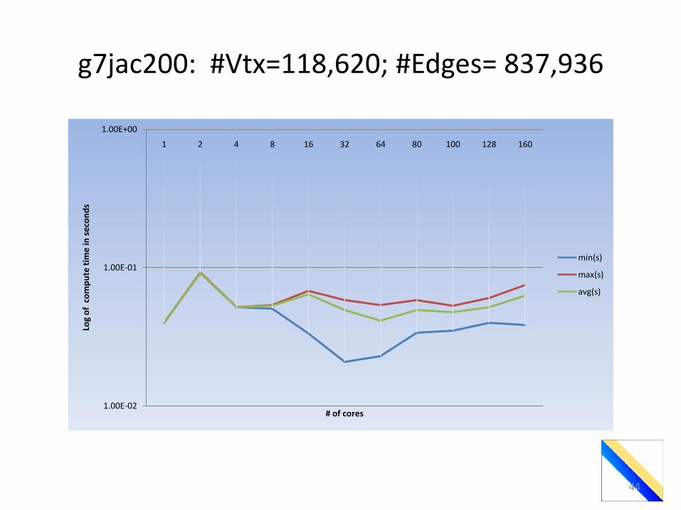
g7jac200: #Vtx=118,620; #Edges= 837,936

1.00E-02

1.00E-01

1.00E+00

1 2 4 8 16 32 64 80 100 128 160

Log

of

co

mp

ute

tim

e in

se

con

ds

# of cores

min(s)

max(s)

avg(s)

44

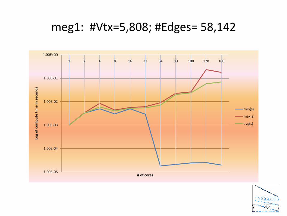
meg1: #Vtx=5,808; #Edges= 58,142

1.00E-05

1.00E-04

1.00E-03

1.00E-02

1.00E-01

1.00E+00

1 2 4 8 16 32 64 80 100 128 160

Log

of

com

pu

te t

ime

in s

eco

nd

s

# of cores

min(s)

max(s)

avg(s)

45

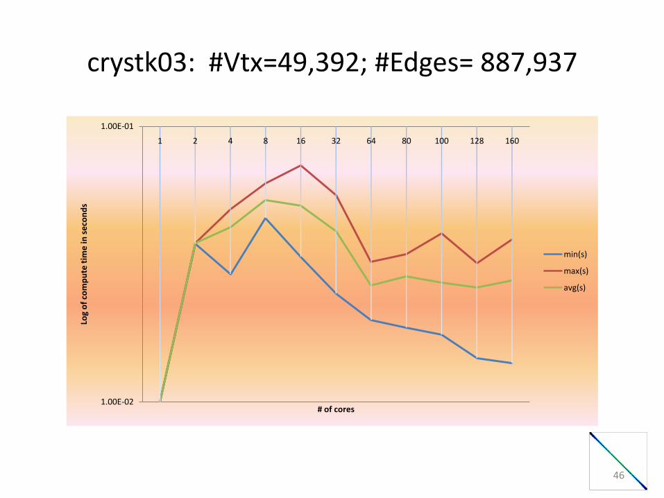
crystk03: #Vtx=49,392; #Edges= 887,937

1.00E-02

1.00E-01

1 2 4 8 16 32 64 80 100 128 160

Log

of

com

pu

te t

ime

in s

eco

nd

s

# of cores

min(s)

max(s)

avg(s)

46

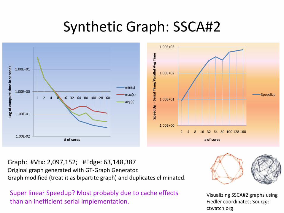
Synthetic Graph: SSCA#2

Graph: #Vtx: 2,097,152; #Edge: 63,148,387Original graph generated with GT-Graph Generator.Graph modified (treat it as bipartite graph) and duplicates eliminated.

Visualizing SSCA#2 graphs using Fiedler coordinates; Source: ctwatch.org

1.00E-02

1.00E-01

1.00E+00

1.00E+01

1 2 4 8 16 32 64 80 100 128 160

Log

of

com

pu

te t

ime

in s

eco

nd

s

# of cores

min(s)

max(s)

avg(s)

1.00E+00

1.00E+01

1.00E+02

1.00E+03

2 4 8 16 32 64 80 100 128 160

Spe

ed

Up

= Se

rial

Tim

e/P

aral

lel A

vgTi

me

# of cores

SpeedUp

Super linear Speedup? Most probably due to cache effects than an inefficient serial implementation. 47

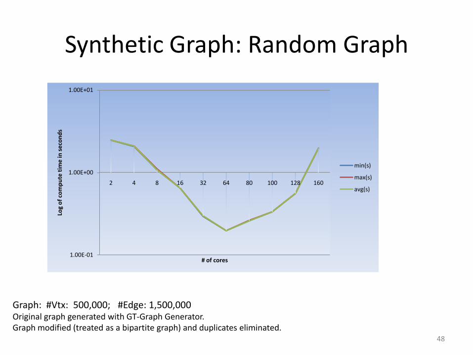
Synthetic Graph: Random Graph

Graph: #Vtx: 500,000; #Edge: 1,500,000Original graph generated with GT-Graph Generator.Graph modified (treated as a bipartite graph) and duplicates eliminated.

1.00E-01

1.00E+00

1.00E+01

2 4 8 16 32 64 80 100 128 160

Log

of

com

pu

te t

ime

in s

eco

nd

s

# of cores

min(s)

max(s)

avg(s)

48

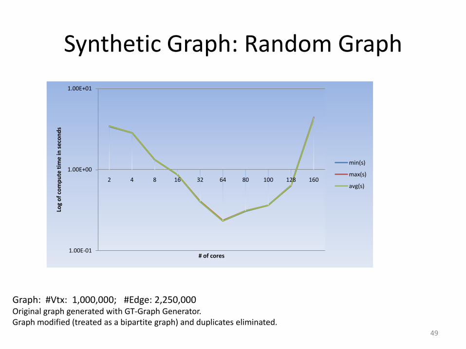
Synthetic Graph: Random Graph

Graph: #Vtx: 1,000,000; #Edge: 2,250,000Original graph generated with GT-Graph Generator.Graph modified (treated as a bipartite graph) and duplicates eliminated.

1.00E-01

1.00E+00

1.00E+01

2 4 8 16 32 64 80 100 128 160

Log

of

com

pu

te t

ime

in s

eco

nd

s

# of cores

min(s)

max(s)

avg(s)

49

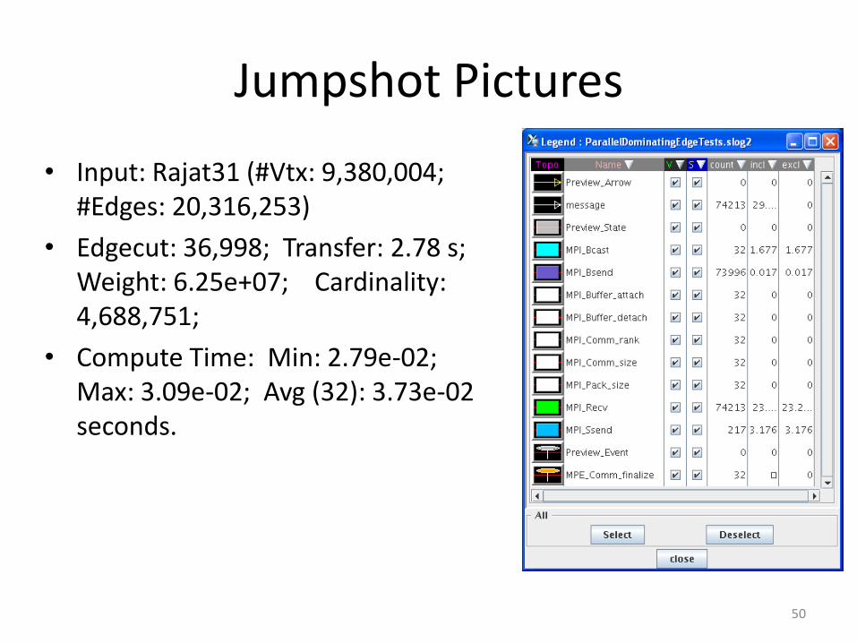
Jumpshot Pictures

• Input: Rajat31 (#Vtx: 9,380,004; #Edges: 20,316,253)

• Edgecut: 36,998; Transfer: 2.78 s; Weight: 6.25e+07; Cardinality: 4,688,751;

• Compute Time: Min: 2.79e-02; Max: 3.09e-02; Avg (32): 3.73e-02 seconds.

50

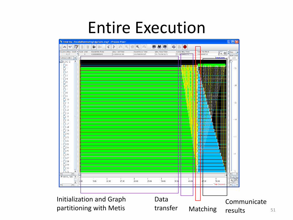
Entire Execution

Initialization and Graph partitioning with Metis

Data transfer Matching

Communicate results 51

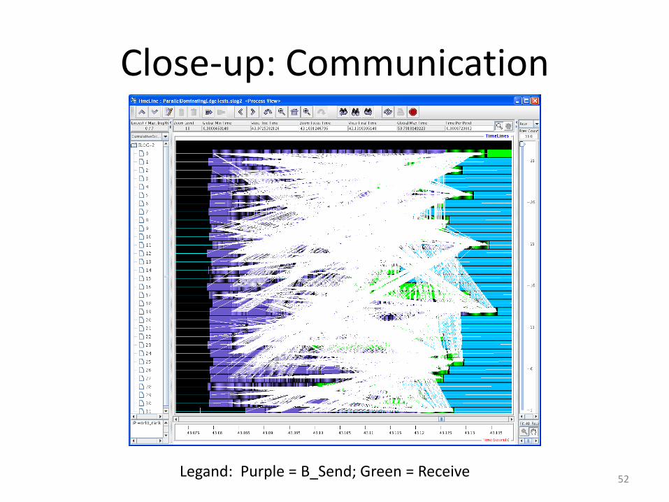
Close-up: Communication

Legand: Purple = B_Send; Green = Receive52

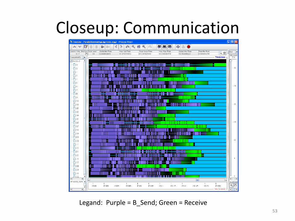
Closeup: Communication

Legand: Purple = B_Send; Green = Receive53

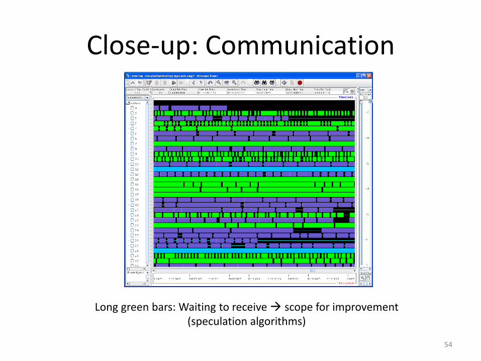
Close-up: Communication

Long green bars: Waiting to receive scope for improvement (speculation algorithms)

54

Outline

1. Introduction





55

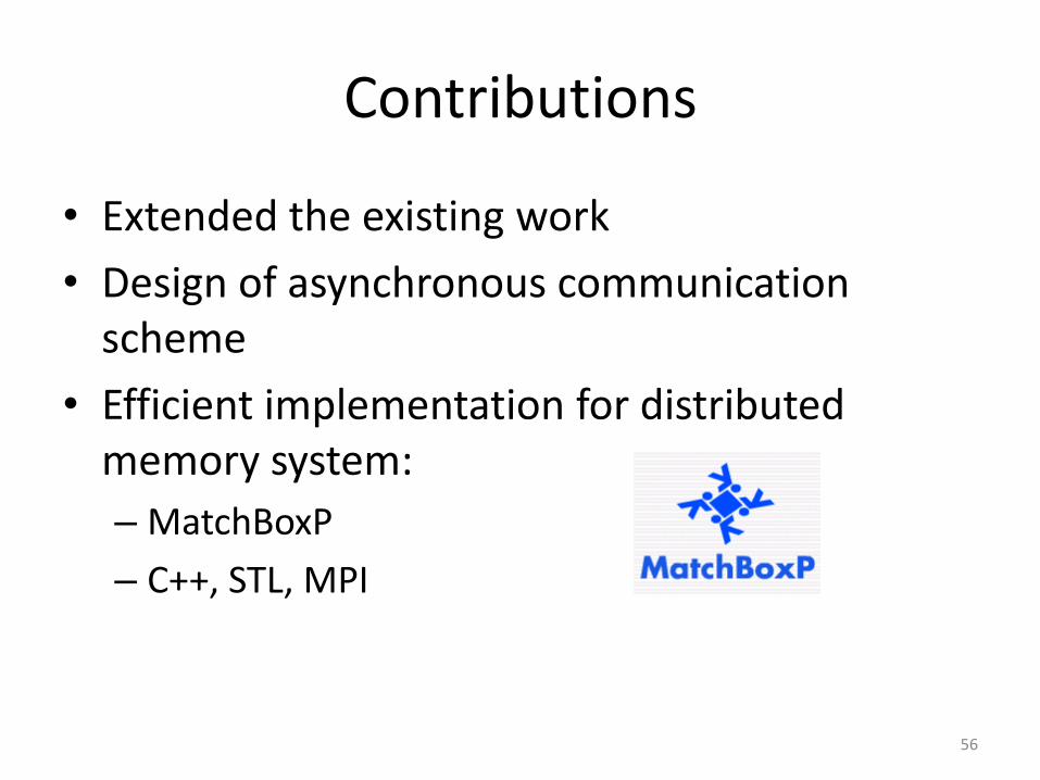
Contributions

• Extended the existing work

• Design of asynchronous communication scheme

• Efficient implementation for distributed memory system:

– MatchBoxP

– C++, STL, MPI

56

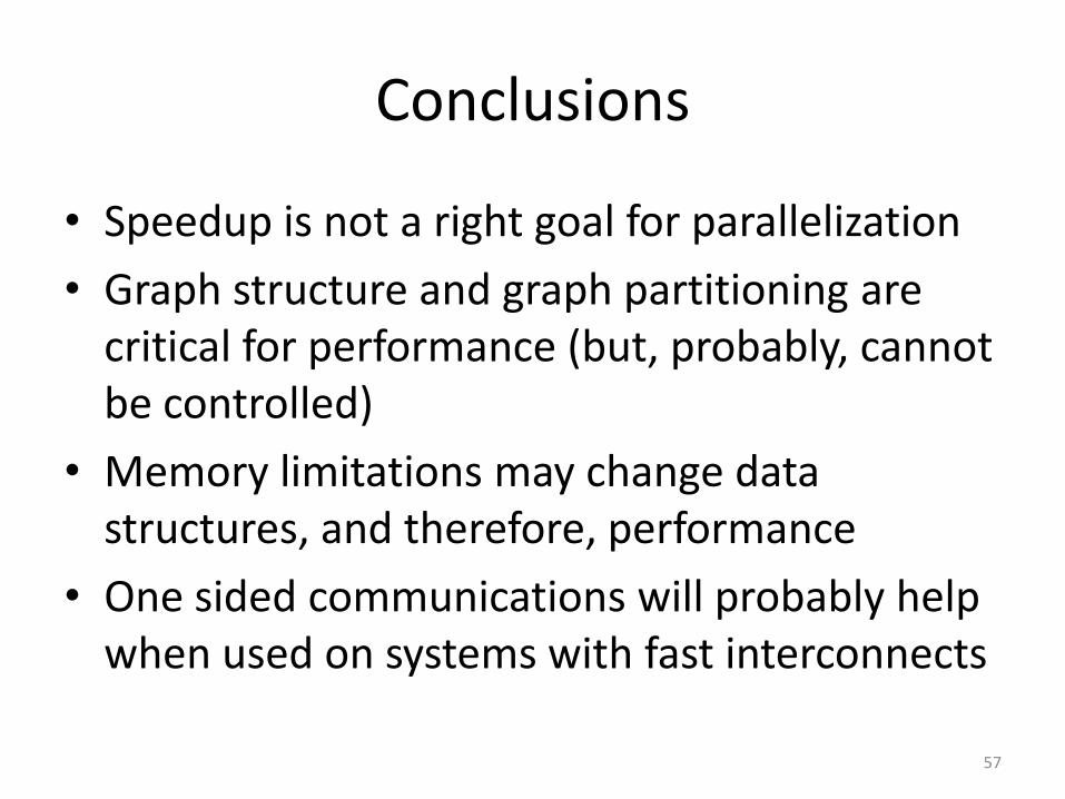
Conclusions

• Speedup is not a right goal for parallelization

• Graph structure and graph partitioning are critical for performance (but, probably, cannot be controlled)

• Memory limitations may change data structures, and therefore, performance

• One sided communications will probably help when used on systems with fast interconnects

57

Future Work

• Tests for performance on the DOE Leadership-class machines (NERSC)

• Massive graphs

• Software engineering: data structures, error handling, documentation, etc.

THANK YOU !

We would like to thank Assefaw Gebremedhin for his time and suggestions to improve this work.

58

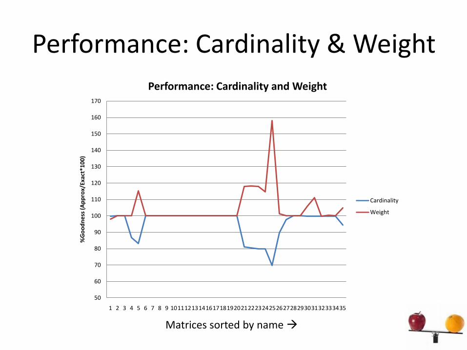
Performance: Cardinality & Weight

50

60

70

80

90

100

110

120

130

140

150

160

170

1 2 3 4 5 6 7 8 9 10111213141617181920212223242526272829303132333435

%G

oo

dn

ess

(A

pp

rox/

Exac

t*1

00

)Performance: Cardinality and Weight

Cardinality

Weight

Matrices sorted by name 59

Documents

Parallel ½-approx Weighted Matching Algorithm