FACULTY OF MECHANICAL, MARITIME AND MATERIALS Delft

Delft University of Technology

FACULTY OF MECHANICAL, MARITIME AND MATERIALS ENGINEERING Department of Marine and Transport Technology

Mekelweg 2 2628 CD Delft the Netherlands Phone +31 (0)15-2782889 Fax +31 (0)15-2781397 www.mtt.tudelft.nl

This report consists of 105 pages and 12 appendices. It may only be reproduced literally and as a whole. For commercial purposes only with written authorization of Delft University of Technology. Requests for consult are only taken into consideration under the condition that the applicant denies all legal rights on liabilities concerning the contents of the advice.

Specialization: Production Engineering and Logistics

Report number: 2012.PEL.7721

Title: Repair process improvement of

Positioning Modules at the AM-WSN

workcenter of ASML

Author: A.R. Dorrepaal

Reparatie-proces verbetering van Positioning Modules in het AM-WSN workcenter van ASML

Assignment: Master thesis

Confidential: yes (until Nov 12, 2017)

Initiator (university): Prof.dr.ir. G. Lodewijks

Initiator (company): Ir. J. Bonsel (ASML, Veldhoven)

Supervisor: Dr. ir. H.P.M. Veeke

Date: November 12th, 2012

Delft University of Technology

FACULTY OF MECHANICAL, MARITIME AND MATERIALS ENGINEERING Department of Marine and Transport Technology

Mekelweg 2 2628 CD Delft the Netherlands Phone +31 (0)15-2782889 Fax +31 (0)15-2781397 www.mtt.tudelft.nl

I

Student:

Professor (TUD):

A.R. Dorrepaal

Prof.dr.ir. G. Lodewijks

Assignment type:

Creditpoints (EC):

Master thesis

35

Supervisor (TUD): Dr. ir. H.P.M. Veeke Specialization: PEL

Supervisor (ASML): Ir. J. Bonsel Report number: 2012.PEL.7721

Confidential: Yes, until Nov 12, 2017

Thesis: Repair process improvement of Positioning Modules at the AM-WSN workcenter of ASML

General background

The NXT lithography-machines of ASML consist of several modules. These modules are built together

during final assembly (fasy) in a cleanroom cabin. Before the final assembly phase, the modules are

assembled and qualified in „assy‟-workcenters. One of the modules, called the wafer stage (WS),

consists of a base module and two positioning modules (PM‟s). A series of production steps and

checks is required to produce these PM‟s. These PM‟s are expensive, machine-performance critical and

factory-throughput critical parts but also very sensitive to disturbances.

The assembly and qualification of the PM requires high effort. Nevertheless, the workcenter of the

PM‟s still faces a fall-out of 32% from the factory. This fall-out is placed back into the system

somewhere, depending on the kind of problem that occurs. This causes a repair flow.

On the one hand, a reduction of this repair is necessary. Many technicians try to realize this. On the

other hand, it is not clear whether the current process of repairing the PM‟s is the optimal. Thereby, it

is required to sustain a moverate of 11 PM‟s/week and meet a delivery performance of 95%, executed

at the lowest possible costs.

Problem statement

Three problems found in relation to the repair flow are stipulated as follows:

1. Unknown economic value of yield improvement

A yield loss of 32% is undesirable high. ASML aims to reduce the yield loss to 12%. However, the

II

economic value of this yield improvement is unclear.

2. Indistinct reject trajectory

There is no strict procedure to reject a PM and return it to the PM workcenter for repair. The process

is un-standardized, based and is fulfilled in different ways. There is often a lack of specific data of the

repaired PM and this leads to confusion and unnecessary communication between the stakeholders.

3. Low delivery performance

Due to a combination of low buffer size, wrong composition, long repair lead time and capacity

shortage the delivery performance does not meet the requirements. Delivery performance suffers

when an above average number of PM‟s is rejected during multiple weeks. Research by simulation will

indicate whether the current capacity is appropriate to handle the severe demand and supply

fluctuations effected by the stochastic pattern of PM rejections.

Research question

In order to solve the problems stated above, the following research question can be formulated:

“Which system design will lead to the best integral workcenter performance, regarding;

moverate;

delivery performance;

costs;

taking into account the repair process of the NXT WS PM production, respecting existing constraints

and resolving known problems?”

Execution

1. Analyze existing processes and system control of the NXT WS PM production at ASML

according the Delft Systems Approach.

2. Quantify these existing processes, including the repair process.

3. Formulate proposals of the current NXT WS PM production, considering the repair process.

4. Design an improved structure, in which build- and repair-PM‟s are processed.

5. Study relevant literature.

Prof.dr.ir. G. Lodewijks Dr. ir. H.P.M. Veeke

------------------------------------- ----------------------------------

III

IV

Preface After many years of hard study at the faculty of mechanical engineering from the TU Delft, I finally

enter the final phase. While successfully completed my bachelor of mechanical engineering, I started

the master specialization Production Engineering and Logistics. After fulfilling the short internship at

Fontijne Grotnes in Vlaardingen, I began my graduation internship in Veldhoven, at the campus site of

ASML. This huge company was a complete new world but soon I found my way in here. Thirsty to an

excellent graduation result I started my project. I spoke to a lot of stakeholders and gathered huge

amounts of data but one question left: How to approach this project? This question finally seemed

harder than expected at first sight and in that way the road to accomplishment was definitely not a

flat one. But I made it. And now I feel proud to present you the final version of my graduation thesis.

I hope you enjoy reading this report as much as I did in compiling it.

Regarding to the content of my graduation thesis I would like to stipulate some important parts. First

of all, the report is divided into three sections: an introduction to ASML, the analysis of the problem

and the solution section. One who‟s interesting in ASML in general should definitely read the

introduction section. The analysis part starts with zooming in to the PM production process in chapter

4. In chapter 5 mainly production and buffer control is analyzed and in chapter 6 the production

resources and capacities are analyzed. The solution section first gives an introduction to the solutions

in chapter 8, then explains the qualitative solution of the reject trajectory in chapter 9. Chapter 11 and

12 shows the verification, validation and confidence analysis. Chapter 13 finally shows the results and

the analysis of the results, in which I came up with some solid recommendations.

I enjoyed very good support from my mentors. Therefore I would like to thank Hans Veeke from the

TU and Joris Bonsel and Herman Vrolix from ASML for their support and good advices.

Onward!

V

VI

Summary An introduction is given of the company ASML, the history of ASML and the products developed by

ASML. One of the product families is the current volume-product: the NXT lithography system. This

machine is composed out of multiple main modules. One of these main modules is the waferstage. On

this waferstage the wafers are moved in the correct position in order to expose them. The waferstage

consists of a base module and two positioning modules (PM‟s). These PM‟s are expensive, machine-

performance critical and factory-throughput critical parts but also very sensitive to disturbances. Due

to the combination of a high disturbance-sensitivity and ASML‟s strategy for a short time-to-market,

the factory faces a high fallout of PM‟s of about 32%. This fall-out is noticed as a yield-loss and

inevitably results in a repair flow of PM‟s.

The production and reparation of PM‟s are situated in the PM workcenter. The requirements regarding

this production system are to be able to fulfill a moverate (output) of 11 PM‟s per week with a delivery

performance of 95%. This must be executed against the lowest variable costs possible. At this

moment, the moverate of 11 PM‟s per week is met, but with an 82% delivery performance. So, the

delivery performance requirement is not met. This low delivery performance is partly caused by the

32% yield-loss.

A yield-loss of 32% is undesirably high. ASML aims to reduce the yield loss to 12%. But the economic

value of this yield improvement is unclear. Costs of an improvement project are easy to determine,

but a sound trade-off can only be made if the economic value of yield improvements are quantified.

The PM production/reparation system has been analyzed in a qualitative and quantitative manner

regarding the production structure, the process control and the production resources. From this

analysis it became clear that a combination of root causes results in the 82% delivery performance. A

buffer of 10 PM‟s on average is used. This buffer exists of four different types of PM‟s. On the moment

a repair PM is rejected, a demand arises immediately. To fulfill the demand created by the rejected

PM a PM from the buffer is consumed. This creates the situation of a lower buffer for the time being

the rejected PM is repaired. The buffer has to cover variability between demand and supply with a

temporary lower buffer size. Besides of that, the correct composition of the buffer is hard to maintain

when control this buffer based on a number of PM‟s. Also, when an above average number of PM‟s

are rejected during multiple weeks, capacity problems occur, with the result that a large part of the

PM‟s are consumed from the buffer. Thus, the combination of a long repair PM throughput time, a

wrong composition of the buffer, a too small buffer size and capacity shortage results in lower than

required delivery performance.

Beside of the problems of the low delivery performance, also problems at the reject trajectory occur.

There is no strict procedure to reject a PM from testrig or test and return it back to the PM workcenter

VII

to repair it. The process is unstandardized and fulfilled in different ways. There is often a lack of

specific data of the repaired PM. This leads to confusion and unnecessary communication between the

stakeholders and PM‟s waiting to become repaired. By performing a study to the required processes,

additional process control and the required information for every repair PM, a real-time dashboard has

been designed. This dashboard indicates the status of every repair PM and the information which still

needs to be gathered.

By using a time-buffer instead of a piecewise buffer the buffer size and composition of the buffer will

be better controllable. Separation of production of regular PM‟s and reparation of rejected PM‟s might

lead to a reduced lead-time of rejected PM‟s. By applying configurations of an increased number of

workstations and operators, research can be done in order to determine the optimal capacity. Multiple

scenarios are defined by means of the parameters described above. The results of these scenarios are

created by means of simulation. In order to be able to simulate, a simulation model is developed,

verified, validated and executed. The results of the simulations are statistically analyzed by means of a

confidence analysis.

From the results it became clear that adding one extra workstation to the bottleneck process, adding

two extra operators to the integration operator team and start the production of every regular PM 28

days before the planned demand date, will result in a delivery performance of 95% with the lowest

variable costs possible. But after studying the data from the confidence analysis it has to be concluded

that there‟s not a statistically significant difference between this configuration and other

configurations.

Recommendations can be done in terms of rules-of-thumb. Two rules-of-thumb are designed. The

occupancy rate of operators has to be in the range of 78±5%. This results in the optimal delivery

performance-costs curve. To reach a delivery performance of 95% within this curve, the correct start

moment needs to be determined. This can be determined by using the second rule-of-thumb. The

start moment consists of a constant of 17 days and a variable part which linearly increases with the

yield-loss. Subsequently the startmoment needs to be scaled to the total workcontent per PM.

Besides of the development of these rule-of-thumbs it is also determined which economic gains will be

made if the yield-loss is reduced from 32% to 12%. When one assumes a production of regular PM‟s

between 4 PM‟s per week (f.e. due to an economic downturn) and 7.4 PM‟s per week (current

situation) then a yearly cost reduction between 941k euro and 1741k euro will be realized.

VIII

Summary (Dutch) Er is een introductie gegeven van het bedrijf ASML, de geschiedenis van ASML en de producten die

door ASML in de loop der tijd zijn ontwikkeld. Eén van de productfamilies is het huidige volume-

product: de NXT lithografie-machine. Deze machine is opgebouwd uit meerdere modules. Éen van de

modules is de waferstage. Op deze module worden de wafers gepositioneerd voor belichting. De

waferstage is opgebouwd uit een base module en twee positioning modules (PM‟s). De PM‟s zijn

kritische onderdelen met betrekking tot de machine-prestaties en de fabrieksdoorlooptijd. Daarnaast

zijn de PM‟s uiterst gevoelig voor verstoringen.Door deze hoge storingsgevoeligheid en de strategie

van ASML om producten zo snel mogelijk in de markt te zetten, vindt er een hoge uitval van PM‟s

plaats (32% van de uitvoer). Deze uitval resulteert in een reparatiestroom van PM‟s.

De productie en reparatie van PM‟s vinden plaats in het PM workcenter. Het workcenter heeft de eis

om een totale uitvoer van 11 PM‟s per week mogelijk te maken tegen een leverbetrouwbaarheid van

95%. Daarbij dienen de variabele kosten per PM zo laag mogelijk gehouden te worden. Op dit

moment wordt er wel een uitvoer van 11 PM‟s per week behaald maar de leverbetrouwbaarheid blijft

steken op 82%. Dit wordt mede veroorzaakt door het hoge yield verlies van 32%.

Een yield verlies van 32% wordt door ASML gezien als onacceptabel hoog. Het is echter onduidelijk

welk economisch voordeel het heeft om dit verlies terug te dringen. De kosten van een

verbeterproject zijn vrij eenvoudig te bepalen, maar om een juiste afweging te kunnen maken zullen

ook de kostenbesparingen van yield-verlies reducties moeten zijn gekwantificeerd.

Het productiesysteem van de PM‟s is kwalitatief en kwantitatief geanalyseerd met betrekking tot de

productiestructuur, de procesbeheersing en de productiemiddelen. Uit de analyse wordt duidelijk dat

er een combinatie van oorzaken aan te wijzen is voor de te lage leverbetrouwbaarheid. Op dit

moment wordt er een stuksbuffer gehanteerd van gemiddeld 10 PM‟s. Deze buffer bestaat uit vier

verschillende types PM‟s. Op het moment dat er een reparatiemodule geretourneerd wordt, ontstaat

er per direct een vraag. Deze vraag wordt ingevuld door een PM uit de buffer. Zo lang de te repareren

PM in het productiesysteem onderweg is, moeten de variaties in het systeem met een kleinere

buffergrootte opgevangen worden. Daarnaast wordt het behouden van de juiste samenstelling

bemoeilijkt door een stuksbuffer te hanteren. Als er gedurende meerdere weken een bovengemiddeld

aantal PM‟s teruggevoerd wordt naar het workcenter, ontstaan er capaciteitsproblemen, met als

gevolg dat de buffer leeggeconsumeerd wordt. De te lage leverbetrouwbaarheid wordt dus

veroorzaakt door een combinatie van een te lange doorlooptijd van de reparatiemodules, een

verkeerde samenstelling van de buffer, een te kleine buffergrootte en capaciteitstekort.

De doorlooptijd van de reparatiemodules wordt niet alleen veroorzaakt door het reparatieproces, maar

ook door het traject van het moment tot afwijzing op de machine totdat de daadwerkelijke reparatie

IX

plaats vindt. Er zijn geen duidelijke afspraken en het is onduidelijk welke informatie benodigd is voor

de reparatie van een PM. Door het opzetten van een kwalitatief proces is vastgelegd welke

processtappen in welke volgorde door welke betrokken afdelingen uitgevoerd moeten worden. Ook is

onderzocht welke informatie benodigd is op welk tijdstip. Dit heeft geleidt tot een real-time

dashboard, welke per reparatie-PM aangeeft wat de status is en welke informatie nog verstrekt moet

worden.

Door een tijdsbuffer per reguliere PM in te bouwen en geen stuksbuffer aan te houden kan de

buffergrootte en samenstelling beter worden beheerst. Door de productie- en reparatiestroom te

scheiden kan er een reductie van de doorlooptijd van reparatiemodules gerealiseerd worden. Door

configuraties met toenemende werkstations en operators toe te passen kan onderzocht worden wat

de capaciteit is. Er zijn meerdere scenario‟s gemaakt aan de hand van bovengenoemde parameters.

Resultaten van deze scenario‟s zijn gecreëerd met behulp van simulatie. Hiervoor is een

simulatiemodel ontwikkeld, geverifieerd, gevalideerd en uitgevoerd. De resultaten van de simulaties

zijn vervolgens statistisch beoordeeld aan de hand van een betrouwbaarheidsanalyse.

Uit de resultaten bleek dat het scenario waarbij er één werkstation aan de bottleneck wordt

toegevoegd, er twee extra operators aan het integratie operator-team deelnemen en er bij elke

reguliere PM 28 dagen voor het geplande vraagmoment gestart wordt met productie, de

leverbetrouwbaarheid van 95% gehaald wordt tegen de laagst mogelijke variabele kosten per PM.

Echter, na bestudering van de gegevens uit de betrouwbaarheidsanalyse blijkt dat er geen statistisch

significant verschil aangetoond kan worden tussen deze configuratie en andere configuraties.

Een aanbeveling kan wel gedaan worden in termen van vuistregels. Er zijn twee vuistregels

ontworpen, met betrekking tot de bezettingsgraad van de operators en met betrekking tot het

startmoment. De optimale bezettingsgraad van de operators blijkt zich te vormen rond 78±5%.

Hiermee wordt de optimale leverbetrouwbaarheid-kosten curve bereikt. Om vervolgens binnen deze

curve een leverbetrouwbaarheid van 95% te behalen, dient het startmoment bepaald te worden.

Hiervoor is een tweede vuistregel opgesteld. Het startmoment bestaat uit een constant deel van 17

dagen en een variabel deel wat lineair oploopt met het yield-verlies. Vervolgens dient het startmoment

geschaald te worden naar de werkinhoud.

Naast de bepaling van deze vuistregels is ook bepaald wat de economische voordelen zijn van een

yield-verlies reductie van 32% naar 12%. Als men uitgaat van een productie van reguliere PM‟s tussen

4 PM‟s per week (bijv. door een economische terugval) en 7.4 PM‟s per week (huidig) dan worden er

jaarlijks tussen de 941k euro en 1741k euro aan kosten bespaard.

X

Glossary 12NC Twelve digit Numerical Code

AM-WSN Assembly Mechanical - WaferStage NXT

ASML Advanced Semiconductor Materials Lithography

assy Assembly phase of modules

BAMO Base Module

BCL Base Capacity Level

BE Business Engineering

BT Buffer Time

CB Carrier base

CIP Continuous Improvement Process

COG Cost Of Goods

CR Crash Rim

CT Cycle Time

D&E Development & Engineering

DN Disturbance Notification

DP Delivery Performance

DRB Disturbance Review Board

ERP Enterprise Resource Planning

EUV Extreme Ultra Violet light

fasy Final assembly phase complete system

INT Integration

LEX Left Exposure Chuck

LOS motor Long Stroke motor

LT Lead Time

ME Manufacturing Engineering

MH Material Handling

MM Means & Methods

Moverate Output (defined by # PM‟s/week)

MQ Manufacturing Quality

NXE NXT with EUV

NXT New Generation Twinscan (platform)

OL Output Leader

PCCSIM Problem, Containment, Cause, Solution, Implementation, Monitor

PCS Problem Cause Solution

PIT Performance Improvement Team

PM Positioning module

PMint2BM Integration of PM to the BAMO

PMQT Positioning Module Quality Test

PP Production Planning

PRO Program Management

REF Refurbishment

RFF Rolling Financial Forecast

REX Right Exposure Chuck

SAPIR Scope, Action, Plan, Implement, Results

SCE Supply Chain Engineering

SS motor Short Stroke motor

TL Team leader

TOPS Technical OPerationS Coördinator

TR Testrig

WIP Work in Progress

WACC Weighted Average Cost of Capital

WS Waferstage

XI

XII

Table of contents

Preface .................................................................................................................................... IV

Summary ................................................................................................................................. VI

Summary (Dutch) .................................................................................................................. VIII

Glossary ................................................................................................................................... X

Table of contents .................................................................................................................... XII

I. Introduction

1. General introduction ASML ..................................................................................................... 3

1.1. Company ....................................................................................................................... 3 1.2. History ........................................................................................................................... 3

1.3. Moore‟s law .................................................................................................................... 4

2. Lithography systems of ASML ................................................................................................. 7

2.1. Wafers ........................................................................................................................... 7 2.2. Lithography .................................................................................................................... 8

2.3. Waferstage .................................................................................................................... 9

2.4. Positioning Module .......................................................................................................... 9

3. Rework ................................................................................................................................13

3.1. Description ....................................................................................................................13 3.2. Effects of yield loss ........................................................................................................13

3.3. Goal and requirements ...................................................................................................14

3.3.1. Goal .......................................................................................................................14 3.3.2. Required performance .............................................................................................16

3.4. Conclusion ....................................................................................................................16

II. Analysis

4. Depiction of the „assemble WS‟-function .................................................................................21

4.1. Aggregation layer 0: black box .......................................................................................21 4.2. Aggregation layer 1: material flow ..................................................................................21

4.3. Aggregation layer 2: „assemble WS‟ ................................................................................22

4.4. The economic value of a yield improvement ....................................................................23 4.5. Conclusion ....................................................................................................................25

5. „Assemble PM‟-function .........................................................................................................27 5.1. Functional structure .......................................................................................................27

5.2. Quantification of repair flow ...........................................................................................27 5.3. Planning & Control .........................................................................................................29

5.3.1. Process control .......................................................................................................29

5.3.2. Function control ......................................................................................................30 5.3.3. Buffer size and delivery performance .......................................................................31

5.4. Indistinct handling of rejected PM‟s .................................................................................35 5.5. Conclusion ....................................................................................................................36

6. Production structure of „Assemble PM‟....................................................................................39

6.1. Functional structure .......................................................................................................39 6.2. Production structure ......................................................................................................40

6.3. Capacity ........................................................................................................................41 6.3.1. Workstations ..........................................................................................................41

6.3.2. Operators ...............................................................................................................43

6.4. Effect of the repair flow .................................................................................................44 6.5. Conclusion ....................................................................................................................46

7. Problem statement ...............................................................................................................49

XIII

III. Solution

8. Solution directions ................................................................................................................53 8.1. Solution method ............................................................................................................53

8.2. Experimental design ......................................................................................................53

9. Qualitative feed forward control for rejected PM‟s ...................................................................57

9.1. Introduction ..................................................................................................................57

9.2. Solution ........................................................................................................................57 9.3. Execution ......................................................................................................................61

10. Simulation model ................................................................................................................63 10.1. Introduction ................................................................................................................63

10.2. Process description language ........................................................................................65

10.3 Cost function ................................................................................................................68

11. Verification & Validation ......................................................................................................69

11.1. Verification ..................................................................................................................69 11.1.1. Introduction..........................................................................................................69

11.1.2. Visualization .........................................................................................................69

11.1.3. Tracing .................................................................................................................71 11.1.4. Calculations ..........................................................................................................73

11.2. Validation ....................................................................................................................78

12. Confidence analysis ............................................................................................................81

12.1. Introduction ................................................................................................................81 12.2. Total variable costs ......................................................................................................81

12.3. Delivery performance ...................................................................................................82

12.4. Conclusion ...................................................................................................................82

13. Results ...............................................................................................................................83

13.1. Introduction ................................................................................................................83 13.2. As-is ...........................................................................................................................83

13.3. Increasing delivery performance ...................................................................................85

13.3.1. Results .................................................................................................................85 13.3.2. Comparing the scenarios .......................................................................................91

13.3.3. Robustness ...........................................................................................................92 13.3.4. Rule-of-thumb occupancy rate ...............................................................................94

13.4. Reducing yield-loss ......................................................................................................95 13.4.1. Introduction..........................................................................................................95

13.4.2. Results .................................................................................................................95

13.4.3. Rule-of-thumb startmoment ..................................................................................98 13.4.4. Conclusion ............................................................................................................99

14. Conclusions ...................................................................................................................... 101

15. Recommendations ............................................................................................................ 103

References ............................................................................................................................. 105

List of figures ......................................................................................................................... 107

List of tables .......................................................................................................................... 109

IV. Appendix

Appendix A – Scientific paper .................................................................................................. 112

Appendix B – Swimming lane reject PM flow ............................................................................ 119

Part 1: escalation flow and reject flow ................................................................................. 119 Part 2: return flow and analyze / repair flow ........................................................................ 120

Appendix C – Dashboard of rejected PM‟s ................................................................................ 121

XIV

Appendix D – Scrap ................................................................................................................ 122

Appendix E – Effective available manpower .............................................................................. 123

Appendix F – Disturbance management ................................................................................... 124

Appendix G - Disturbance duration .......................................................................................... 128

Appendix H - Initialization time of the model ............................................................................ 131

Appendix I - Inter arrival time distribution................................................................................ 132

Appendix J – input of the simulation model .............................................................................. 133

Appendix K – Occupancy rates of workstations ......................................................................... 139

Appendix L – output of the experiments .................................................................................. 140

Appendix M – confidence analysis ........................................................................................... 151

XV

1

I. Introduction

2

3

1. General introduction ASML

1.1. Company ASML is one of the world's leading providers of lithography systems for the semiconductor industry,

manufacturing complex machines that are critical to the production of integrated circuits or

microchips. Headquartered in Veldhoven, the Netherlands, ASML designs, develops, integrates,

markets and services these advanced systems, which continue to help customers - the major

chipmakers - reduce the size and increase the functionality of microchips, and consumer electronic

equipment.

1.2. History Founded in 1984 as a joint venture of Philips and ASM International, the production of the first

stepper systems (called PAS, Philips Automatic Stepper) were realized. Within a year ASML grew to

100 employees and ASML moved from Eindhoven to an office in Veldhoven. In 1987, ultraviolet light

was used in the PAS2500. With this technique, prints could be made with details of 0.7 micrometer.

This machine was followed by the PAS5000, which realized details of 0.5 micrometer in 1989 and

0.35 micrometer in 1991. In 1993 the production of step-and-scan machines started, which lead to a

higher throughput of the wafers. In 2001, lithography-machines of ASML were also equipped with an

ArF-laser source. This light made it able to realize better imaging on wafers.

During the 21st century, the techniques in the ASML lithography-machines are increasing rapidly. In

2006, the TWINSCAN XT is considered as a volume-product, with over 250 shipping‟s a year.In 2007,

imaging of 36.5nm is possible by the XT1900i. Also the immersion technique in twinscan is starting to

become volume, with 60 immersion-systems sold this year. In 2008, a new platform is introduced:

the TWINSCAN NXT: The new platform brings overlay and productivity breakthroughs: it addresses

technical and economic challenges in a holistic way, enabling a more seamless adoption of double

patterning.

In the years after 2008 the current systems are sold more often, but also another technique is

introduced: NXE-machines with EUV. This enables smaller imaging, due to the Extreme Ultraviolet

laser beam. Nowadays, the NXE systems are in pilot phase with a dozen sold, but parallel to

developing the design, the system will be pushed to the market.

Also a strong increase in market share is realized, up to 80% market share nowadays. The reason for

this success is the result of focus on modularity of the lithography systems and short time to market.

4

Figure 1 - ASML products

1.3. Moore’s law Every digital electronic device (mobile phones, laptops, usb-sticks, etc.) consist of chips. During the

existence of chips, the power, cost and time required for every computation done by these chips is

highly reduced. This is a result of the reduction of the size of these chips.

Figure 2 - Moore's law

5

Nowadays, Integrated Circuits (IC‟s) can be built together by imaging, which result in a high amount

of transistors on a small area. The trend in the past 40 years was first observed by Intel co-founder

Gordon Moore and is referred to as „Moore‟s Law‟. Moore‟s Law states that every two years the

computational capacity of a chip is doubled. Until now this is reality, but to contain this law in future,

ASML focuses on developing new techniques on a high speed and serves his customers with the

systems consisting of these techniques.

6

7

2.Lithography systems of ASML

2.1. Wafers Several processes are necessary to create IC‟s. The core processes are shown in Figure 3. Wafers are

composed of crystalline silicium. Oxidation of the silicium is the first step, which creates an isolated

layer. Then a photoresist layer is formed. This layer is a photoresist to make it able to apply

lithography.

Figure 3 - IC manufacturing

8

The light is brought onto the wafer by a pattern. A pattern is created in the photoresist layer. This

gives the possibility to etch the silicium oxide where it has to conduct. These steps are repeated

several times to create a series of layers with complex structures. In this way billions of transistors

are created in the semiconductor material of the wafer.

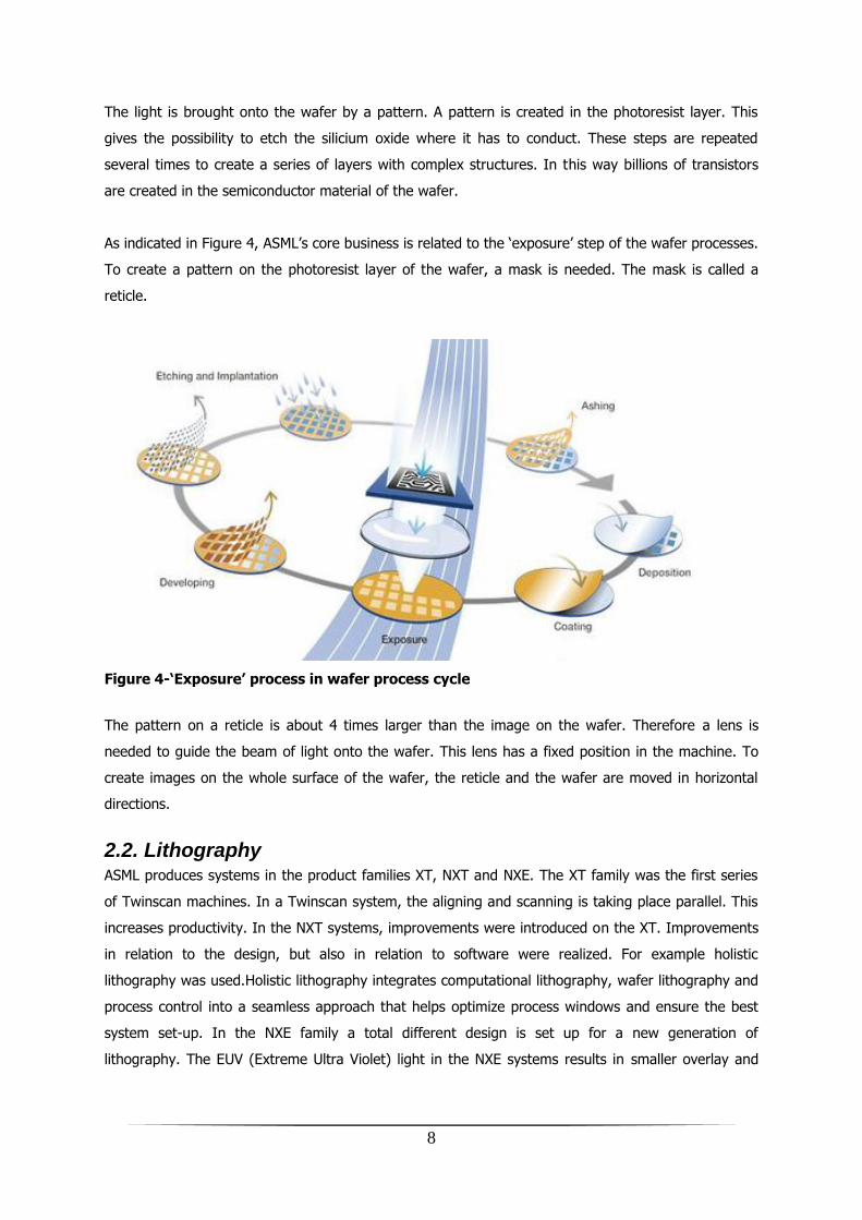
As indicated in Figure 4, ASML‟s core business is related to the „exposure‟ step of the wafer processes.

To create a pattern on the photoresist layer of the wafer, a mask is needed. The mask is called a

reticle.

Figure 4-‘Exposure’ process in wafer process cycle

The pattern on a reticle is about 4 times larger than the image on the wafer. Therefore a lens is

needed to guide the beam of light onto the wafer. This lens has a fixed position in the machine. To

create images on the whole surface of the wafer, the reticle and the wafer are moved in horizontal

directions.

2.2. Lithography ASML produces systems in the product families XT, NXT and NXE. The XT family was the first series

of Twinscan machines. In a Twinscan system, the aligning and scanning is taking place parallel. This

increases productivity. In the NXT systems, improvements were introduced on the XT. Improvements

in relation to the design, but also in relation to software were realized. For example holistic

lithography was used.Holistic lithography integrates computational lithography, wafer lithography and

process control into a seamless approach that helps optimize process windows and ensure the best

system set-up. In the NXE family a total different design is set up for a new generation of

lithography. The EUV (Extreme Ultra Violet) light in the NXE systems results in smaller overlay and

9

imaging accuracies and higher throughput. In this report the subject is the waferstage of the NXT

system.

The lithography systems of ASML do have a strong modular composition. The laser light has to travel

through several modules of the machine. In figure 3 some of the parts are pointed. The light is

created outside the machine and enters at the light entrance. The light travels through the

illumination system via several mirrors and lenses to create the optimal composition of the light. After

that, the light crosses the reticle stage and leaves the reticle stage patterned. In the lens, the light

bundle is made four times smaller and is focused onto the wafer, creating the pattern on the wafer.

The wafer is supported and moved by the waferstage.

Figure 5 - lithography machine

2.3. Waferstage The main purpose of the wafer stage is to exchange the wafer with the wafer handler, and accurately

position the wafer for exposure. In order to accomplish this, the waferstage processes two wafers in

parallel, one on the exposure side and one on the measure side. This is shown in Figure 6. The main

components of the NXT wafer stage are the base frame (BAMO) and the two positioning modules

(PM).

2.4. Positioning Module On a waferstage always two positioning modules are present, a LEX (left-side positioning module)

and a REX (right-side positioning module). The positioning module guides the wafers and

interchanges the wafers between the lens and the wafer handler. The PM is able to freely move,

without physical interaction with the BAMO. This is done by planar motors in the PM. These „long

10

stroke‟ (LS) motors cause movements in x- and y-directions and create a space between the PM and

the BAMO, all realized by magnetic force.

Figure 6 - waferstage

Figure 7 - exploded view PM

11

The base carrier holds the long strokes and the other components. The hose assembly consists of

multiple ducts to supply the other components of water, air and vacuum. The short stroke module is

assembled onto the base carrier, with the hose assembly in between. The short stroke module is used

for fine alignment of the wafer. The measurements are done with multiple alignment lasers. To

protect the PM for impacts due to for example collisions, a crash rim is assembled. On top of the

short stroke module the wafer chuck is assembled. This wafer chuck supports the wafer table. On top

of the wafer table, the wafers can be placed.

The precision of the alignment of the wafer is comparable with shining with a torch to the moon and

hitting a coin on the moon with that light bundle. In the case of the lithography systems, not the

torch is aligned but the coin is aligned. Therefore a minimum of deviations in the components and

assembly of the PM is allowed. Another important issue is the throughput of the lithography systems

and therefore the speed of the PM‟s. As a matter of fact, with the design of lithography systems three

performance indicators of the system are taken into account. The performance of the system is

measured in terms of:

1. Imaging: The quality of the transfer of images from the reticle to the wafer.

2. Overlay: The accuracy with which the system can expose one product layer on top of

another.

3. Throughput: The amount of handled wafers per hour.

Machines nowadays can produce 175 - 200 imaged wafers per hour with an overlay of 2.5nm. This

requires high demands of the lithography system. The wafer stage is a critical module for the

realization of these performances. Working at extremely high speeds, and using an accurate

measuring system, it is capable of achieving high throughput and maintaining high accuracy during

scanning.

Nevertheless does this high performance result in complex modules. And due to this complexity,

continuous improvements in the design are made. Especially the PM‟s consists of a high-tech design.

This leads to fallout of about 30% at the end of the production process sequence. The extreme high

cost-of-goods of a PM results in an inevitable rework of every failed PM.

12

13

3. Rework

3.1. Description Rework cannot be described as a stand-alone system. It is inevitably connected to a certain

production process. As a matter of fact, the rework is caused due to yield losses in the production

process. An example of rework is given by [Flapper, 2002] in Figure 8.

Figure 8 - Example of production-rework process

In this example, it becomes clear that dealing with yield loss can be done in different ways. The failed

products which are not able to become repaired are known as non-reworkable defective products or

scrap. Products which still can be repaired are known as reworkable defective products. The rework

can be realized in two ways, the in-line rework or the off-line rework. In the case of in-line rework the

same resources are used for both the production and the rework. In the case of off-line rework,

dedicated resources are available for the rework only.

3.2. Effects of yield loss As mentioned above, yield and rework are strongly related. In [Bohn/Terwiesch, 1999] some issues

are pointed in relation to rework. Rework as a result of yield loss has a negative influence on capacity

of the process. If rework involves only non-bottleneck processes with a large amount of idle time, the

rework has a negligible effect on the overall process capacity. However in many cases rework is

14

severe enough to make a process a bottleneck. The worst case scenario occurs when the rework

needs to be carried out in the bottleneck process. As known, the overall capacity never exceeds the

bottleneck capacity. Therefore all capacity invested in rework on the bottleneck process is a loss of

capacity from the perspective of the overall process.

Also the variability is influenced by rework. Yield loss never occurs in a deterministic way but in a

stochastic way. Thus, yield losses increase variability and a result of that is a decrease of capacity.

Even if the operation itself is deterministic, when the failed item will immediately be reworked on the

specific workstation it will lead to a random variable processing time of the specific item at the end of

the process sequence.

These capacity losses due to variability can partially be solved by adding and increasing buffers (thus

increasing WIP), especially behind the lower yield processes. Coincide of this measure is; higher costs

with relation to the material (interest) and an increase of overall throughput-time.

Table 1 - Cost effects of yield loss

Concluding, an increase in yield can realize higher capacity with the same production means and

lower variability. Lower variability may increase capacity and gives opportunities to lower the WIP.

Lowering the WIP decreases the costs of capital and shortens the throughput-time. An increase of

available capacity in the regular production process will be realized by creating an off-line rework

process. According to this conclusions it is interesting whether the performance of the workcenter as

a whole increases by using off-line rework or not.

3.3. Goaland requirements

3.3.1. Goal

The waferstages are produced in the AM-WSN workcenter. A sub-center of AM-WSN is the WSN-PM

workcenter. In the WSN-PM workcenter the PM‟s are assembled. The goal of the AM-WSN workcenter

is to assemble waferstages. To realize this goal, several functions within this workcenter need to be

fulfilled. Two of these functions are the „assemble-PM‟ function and the function to rework failed PM‟s,

called the „repair PM‟ function. As mentioned above, several parameters are interesting regarding the

performance of a production process with rework.

cost type yield effect

material-related costs incremental material to replace bad components

labor-related costs rework labor

capacity-related costs more capacity needed in the rework loops of processes

variability-related costs WIP costs to buffer variability

15

As stated in [Bikker, 1992], for the design of a system clear requirements needs to be formulated.

Bikker formulates six process design criteria. Four design criteria are selected in the case of this

rework function. When developing a system for the rework function, decisions needs to be taken on

behalf of the following design criteria:

• effectiveness

• productivity

• reliability

• flexibility

Since the new rework process needs to be seamless adopted in the AM-WSN workcenter, the design

criteria „quality of work‟ and „ability to innovate‟ won‟t be used. The integral solution will ask a way of

working which is comparable with the current way of working in the workcenter. In other words,

decisions on these two requirements are outside the system boundary.

The requirement effectiveness is measured in terms of results. Within the AM-WSN workcenter these

results are expressed in terms of capacity or moverate. The requirement productivity is the ratio of

effectiveness and efficiency. The efficiency is the level of sacrificing means to realize a certain goal

(the results). Within the AM-WSN workcenter this efficiency is expressed in terms of costs. At ASML

these costs are subdivided in material-related costs, labor-related costs and facility-related costs.

Reliability regarding the production of the PM is measured in terms of delivery time reliability. In [In „t

Veld, 1993, p.8] flexibility is explained with relation to different aspects. Important aspects within the

ASML production are the renewal flexibility, the volume flexibility and the organizational flexibility.

The „assemble PM‟ function has to have the capacity to meet the demands and fulfill the demands on

time (delivery performance) by performing against a certain level of costs. Of course, flexibility can be

used to adjust to the right capacity or to reach a specific level of on-time deliveries of the PM‟s when

order patterns are suddenly changing.

With the above, the goal of a rework function at ASML can be described as follows:

The rework function in the AM-WSN workcenter has the main goal to analyze, dismount and

repair failed PM‟s with a minimum of negative impact on the WSN-PM workcenter regarding;

moverate

delivery performance

costs

o labor costs

o capital costs of WIP and buffer

o scrap costs

16

3.3.2. Required performance

ASML want to be able to decide to keep the moverate constant and decrease the work content. It is

required to have a system which is able to act on a moverate of 11 PM‟s/week.

The workcenter produces modules in assy phase. The lithography system consists of multiple

modules. These modules are produced in the workcenters in parallel order. With parallel production,

the performances are multiplied with each other to determine the delivery performance of the

complete litho system. Therefore a high delivery performance is required for every workcenter on its

own. The performance of the delivery time of the workcenter is stated by ASML to be 95%, measured

over a year.

Both the delivery performance and the moverate requirement need to be fulfilled with total variable

costs as low as possible. These costs consist of the components as shown in table 1.

3.4. Conclusion In Figure 9 the parts aggregation is shown as explained in the introduction.

Figure 9 - parts aggregation

Rework can be distinguished in in-line rework and off-line rework. Rework is the effect of yield loss.

Effects of yield change are mentioned. An increase in yield can realize higher capacity with the same

production means and lower variability. Lower variability increases capacity and lowers the WIP.

main module sub-assembly’s

metroframe

…

waferstage

reticle stage

chuck assy

PM (2x)

BaMo

module

carrier base

crash rim

SS motor

hose assy

LOS motors

system

XT

NXT

NXE

17

Lowering the WIP decreases the material costs and shortens the throughput-time. Second, an

increase of yield in the regular production process can be realized by creating an off-line rework

process.

Rework as part of a production process in ASML has a goal which is described as follows:

The rework function in the AM-WSN workcenter has the main goal to analyze, dismount and

repair failed PM‟s with a minimum of negative impact on the WSN-PM workcenter regarding;

moverate

delivery performance

costs

o labor costs

o WIP costs

o facility costs

Requirements are stated as follows:

moverate ≥ 11 PM‟s/week

delivery performance ≥ 95%

lowest costs possible

18

19

II. Analysis

20

21

4. Depiction of the ‘assemble WS’-function

4.1. Aggregation layer 0:black box

Figure 10-Aggregation layer 0: black box ASML

As explained in the introduction, the lithography systems carry a strong modularity. The main

modules are assembled separated from each other and built together to a lithography system in the

final assembly. This implies that in the system „ASML company‟ (see Figure 10) a series of

subsystems are present. One of these subsystems is the assembly of the waferstage. This is shown in

Figure 11.

4.2. Aggregation layer 1: material flow Figure 11 shows the PROPER-model [Veeke, 2007] dedicated to ASML. A zoom-in is shown on the

„produce‟-function within ASML. This subsystem realizes the production of lithography systems. This

subsystem is responsible for the materials flow. It is divided into a sequence of processes to be able

to fulfill the orders in the order flow.

The zoom into the material flow of ASML has been divided in a „module assembly‟-function, a „final

assembly‟-function, a „test‟-function and an „install‟-function. The problem zone is situated within the

„module assembly‟-function. Within this function, the production of the modules of a lithography

system takes place in parallel order. Workcenters are allocated to fulfill the production of a module.

One of the modules, as described in the introduction, is the waferstage (WS). The „assemble WS‟ -

function is fulfilled by the AM-WSN workcenter. Within the „assemble WS‟-function also the positioning

modules are assembled.

requirements performance

orders

materials

resources

performed orders

litho systems

used resources

ASML company

Provide lithography systems

22

Figure 11-Aggregation layer 1: zoom into the material flow

Figure 12 - aggregation layer 2: zoom into ‘assemble WS’

4.3. Aggregation layer 2: ‘assemble WS’ In the AM-WSN workcenter the waferstage is produced. This is done by several build, integrate and

test functions. This is shown in Figure 12. As mentioned in the introduction, the waferstage consists

of a BAMO and two PM‟s. The PM‟s are produced in the „assemble PM‟-function. The entering flows of

this function are materials for new build PM‟s, refurb PM‟s and repair PM‟s. The refurb PM‟s are

assemble

requirements performance

orders

materials

resources

performed orders

litho systems

used resources

materials

materials Assemble WS

CONTROL

standards results

Assemble RS

Assemble …

test install

field returns

yield loss

Assemble WS (AM-WSN)

progressorder

quantities

- required MR

- req.del.perf.

- budget

- CT/ MR,

- costs,

- deliv. perf.

assemble PM integrate

refurb

test

Fa

sy &

tes

t

cu

sto

me

r

23

replaced at the customer and returned to ASML. These PM‟s are upgraded during refurb and then

added to the regular flow into „assemble PM‟. The parts are assembled to a complete integrated and

tested PM and will, together with another PM, be integrated to a BAMO. The PM‟s and BAMO form a

waferstage. This waferstage can either be tested on a testrig or continue immediately to the final

assembly section of ASML. The waferstages which proceed to the testrig are tested. After that, a part

of the PM-sets is de-integrated from the BAMO and delivered to the service department of ASML. The

other part continues to the final assembly (fasy), is integrated in a new NXT lithography system and

tested.

The repair PM‟s are rejected from inside the factory. The rejected PM‟s originate from the testrig

sequences and the tests of the lithography systems. This is indicated by the red arrow in Figure 12.

Refurbish PM‟s and new build PM‟s are considered as one flow for three reasons:

1. Repair PM‟s are originating from both the build flow and the refurbish flow.

2. The refurbishment flow as well as the new build flow both serves the profit of ASML.

Opposite, the costs of the repair flow have to be ascribed to the build and refurbish flow.

The „assemble PM‟-function gets orders from the order flow of ASML and reports progress to the

order flow. The performance of this function is reported to higher echelons. As is discussed in the

introduction, the performance is measured in terms of delivery performance, moverate (output) and

costs.

4.4.The economic value of a yield improvement The output of the PM production system is shown in Figure 13. Except from week 52 (Christmas

holiday), the weeks with a low output of build PM‟s do also have a high output of repair PM‟s. There

appears to be a negative influence of repair PM‟s on the output of regular build PM‟s. This might be

the case when the repair flow consumes a substantial part of the available capacity.

Figure 13 - Output of ‘assemble PM’-function

0

2

4

6

8

10

12

1140 1141 1142 1143 1144 1145 1146 1147 1148 1149 1150 1151 1152 1201 1202 1203 1204 1205 1206 1207 1208 1209

# P

M

Week

Output AM-WSN

build

repair

24

Four types of PM‟s are produced by ASML in the AM-WSN workcenter:

PM311LEX

PM311REX

PM321LEX

PM321REX

The moverate and the yield loss of the PM‟s is determined by counting the number of PM‟s of each

category over the period of week 8 of 2011 to week 8 of 2012. With these data the yield loss per PM

type is determined.

Table 2-Product mix and yield loss

The product mix of the output of the workcenter is determined to be 33% of PM311‟s versus 67% of

the PM321‟s. The consolidated yield loss therefore is determined to be 32%. How this 32% relates to

the other flows of PM‟s through the ASML system is shown in Figure 14.

Figure 14 - flows of PM's

The yield loss originates from the testrig systems (11%) and from the NXT systems which are tested

before being directed to the customer (21%). The 32% of rejected PM‟s are added to the „assemble

PM‟-function together with the 68% of build and refurb PM‟s. This results in the 100% output of the

„assemble PM‟-function. The integration of the PM-sets to a BAMO leads to a 33% flow directly to

fasy. These PM‟s are unqualified because it was chosen not to qualify these PM‟s on a testrig. This

choice is made to reach the required moverate. 67% of the PM flow continues to the testrig tests.

PM311LEX PM311REX PM321LEX PM321REX

build PM's [#] 48 48 93 97

repair PM's [#] 24 19 43 51

total [#] 72 67 136 148

Yield loss [%] 33% 28% 32% 34%

field returns

yield loss

Assemble WS (AM-WSN)

assemble PM integrate

refurb

test

Fa

sy &

test

cu

sto

me

r

9%

33%

47%

68%

32%

11%

100% 67%

21%

21%

25

After this, 47% of the PM‟s is delivered to the service pool. 9% of the PM‟s continues to fasy. ASML

aims to increase the capacity of the testrig process.

In [Bohn/Terwiesch] drivers to reduce yield loss are stipulated. Managerial decisions are driven by the

economic value of a yield improvement. In the case of ASML, especially decisions regarding process

improvements are drivers to understand economic pay-back of yield loss reduction. Whereas the

economic cost of improvement projects can be computed easily, the gains can only be determined by

understanding the economic value of a yield improvement.

A yield loss of 32% is undesirably high. ASML aims to reduce the yield loss to 12%. But the economic

value of this yield improvement is unclear. When allocating budgets, especially budgets for the

development department, a quantification of the cost reduction is necessary. Only with quantifications

of the economic value of yield improvement, clear agreements can be made regarding budgets and

improvement plans of the manufacturing and development department.

4.5. Conclusion The PM‟s of the repair flow are rejected from testrig or test. Together with the regular PM‟s, the

repair PM‟s are processed in the „assemble PM‟-function. This function is represented by the AM-WSN

workcenter. Four types of PM‟s are produced:

PM311LEX

PM311REX

PM321LEX

PM321REX

The product mix of the output of the workcenter is determined to be 33% of PM311‟s versus 67% of

the PM321‟s. The yield loss is determined to be 32%.

In [Bohn/Terwiesch] drivers to reduce yield loss are stipulated. In the case of ASML, especially

decisions regarding process improvements are drivers to understand economic pay-back of yield loss

reduction. A yield loss of 32% is undesirably high. ASML aims to reduce the yield loss to 12%. The


26

27

5. ‘Assemble PM’-function

5.1. Functional structure The „assemble PM‟-function consists of two stages regarding the regular PM flow. First the

subassemblies are built. Then the subassemblies are integrated to a PM. Rejected PM‟s are analyzed

and dismounted. This process of analysis and dismounting is executed with the same resources as

the integration process of the PM. After dismounting, the failed subassemblies are returned to the

„build‟ process. There the subassemblies are repaired. These processes are shown in Figure 15 -

aggregation layer 3: zoom into 'assemble PM'.

Figure 15 - aggregation layer 3: zoom into 'assemble PM'

5.2. Quantification of repair flow In this paragraph the repair flow will be quantified. The number of repair subassemblies will be

specified and the percentages of quick fix orders. The data are measured over a period of one year,

beginning in week 8 of 2011.

After discussions and by data analysis, it became clear that there can be made a distinction between

regular repair PM‟s and quick fix repair PM‟s. The quick fix PM‟s does have the property that it has to

return in exactly the same test sequence as it was originated from. On the other hand, the regular

rejected PM‟s can be replaced by other PM‟s as well. The decision to handle a rejected PM as a quick

fix is based on the progress in the test sequence, the number of PM‟s available on stock, and the

severity of the problem. This last driver implies that quick fix PM‟s do have a smaller work content

than regular repair PM‟s. The quick-fix orders are separated from the regular repair orders based on

the number of operations. Non-quick-fix orders (build as well as repair orders) contain 6 operations:

build

analyze and dismountrejected PM

carrier

base

crash rim

integrate

chuck assy

SS motor

PM

28

1) Integration CB+SS+LOS+CR

2) PMQT1

3) Integration Chuck Assy

4) PMQT2

5) Finalize

6) Final Quality Check

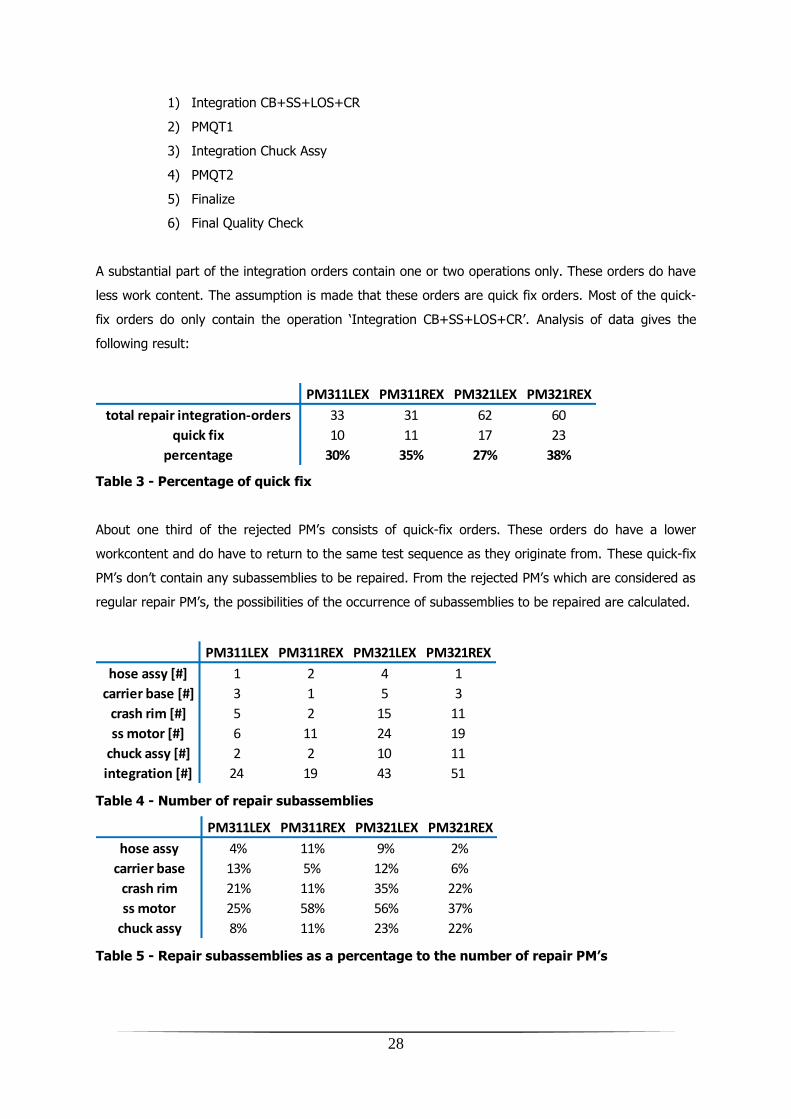
A substantial part of the integration orders contain one or two operations only. These orders do have

less work content. The assumption is made that these orders are quick fix orders. Most of the quick-

fix orders do only contain the operation „Integration CB+SS+LOS+CR‟. Analysis of data gives the

following result:

Table 3 - Percentage of quick fix

About one third of the rejected PM‟s consists of quick-fix orders. These orders do have a lower

workcontent and do have to return to the same test sequence as they originate from. These quick-fix

PM‟s don‟t contain any subassemblies to be repaired. From the rejected PM‟s which are considered as

regular repair PM‟s, the possibilities of the occurrence of subassemblies to be repaired are calculated.

Table 4 - Number of repair subassemblies

Table 5 - Repair subassemblies as a percentage to the number of repair PM’s


total repair integration-orders 33 31 62 60

quick fix 10 11 17 23

percentage 30% 35% 27% 38%


hose assy [#] 1 2 4 1

carrier base [#] 3 1 5 3

crash rim [#] 5 2 15 11

ss motor [#] 6 11 24 19

chuck assy [#] 2 2 10 11

integration [#] 24 19 43 51


hose assy 4% 11% 9% 2%

carrier base 13% 5% 12% 6%

crash rim 21% 11% 35% 22%

ss motor 25% 58% 56% 37%

chuck assy 8% 11% 23% 22%

29

The numbers of repair subassemblies are counted and divided by the total number of regular repair

PM‟s. This results in the percentages as shown in Table 5.

5.3. Planning& Control

5.3.1. Process control

The planning of the production of the PMs is shown in Figure 16 - process control. The order flow is

outside the boundaries of the workcenter but generates orders for the workcenter. These orders

consist of two kinds. On one hand there is the production of new machines, which require new PMs

too. On the other hand, ASML has a service department, which swaps PMs at the customer and asks

for new or refurbished PM‟s at the workcenter. Both of these demands are processed by the planning

control function. Planning control has the task to balance the available moverate of the workcenter

with the required moverate. This is realized by comparing work in progress, stock levels, the number

of required PM‟s, the demand dates of the required PM‟s and the required moverate. The compare

function creates due dates, which are transformed to start dates with information of throughput times

from the function control. Data about throughput times, workcontent and buffer times are reported to

the function control on quarterly basis. Progress is reported to the order flow of ASML on a weekly

basis. This is done during staff meetings.

Figure 16 - process control

PP&C

materials

order quantities

(fasy plan, service demand,

AMSL Twinscan, rejects)progress

order progress,

stock levels

start dates

PM

move rate

(11 PM/w)

due dates

Takted routings

start dates

- actual CT

- actual man-hours

- queue times

assemble

control compare

intervene measurestaff meeting

function control

order progress,

stock levels

30

Figure 17 - quarterly norm review

5.3.2. Function control

The norm review is a reoccurring quarterly function control to evaluate and initiate the correct norms

for takted routings used in the workcenter. This cycle is shown in Figure 17.

Figure 18-Function control

- throughput times

- required moverate

optimum

production

sequenceCT data

CT report

rebalancing

trigger

(at least once per

quarter)

- actual CT

- actual man-hours

- queue times

evaluate

ME (& norm review)

initiate

BE

process control

higher echelon control

31

The norm review will be described by means of Figure 18.The progress of the execution of the

operations is logged in the takt progress monitor. These data are available for the Business

Engineering department, which analyzes these data (at least) every quarter. The result of the analysis

is a report which is used as fixed reference by other functions at ASML. One of these functions is the

norm review meeting. In this meeting, the stakeholders (ME, BE, OL, etc.) review the report data and

compare it with the current norms. When it becomes clear that a part of the production process is

fulfilled in a shorter lead time or requires less labor, the norm is adjusted. This rebalancing result in

takted routings for the production of the PMs and it‟s subassemblies. It contains labor times and lead

times for every step in this production process.

This function control is the norm review, but as can be seen in Figure 18, it is strongly connected to

the process control of the production. Although, this is done on daily basis, and the norm review is

executed only once in a quarter, the process control function needs the output created by the norm

review.

5.3.3. Buffer size and delivery performance

Now first the relation of the moverate with the lead time is explained. Little‟s Law [Slack, 2007] is

stated:

[𝐸𝑞. 5.1] 𝑙𝑒𝑎𝑑 𝑡𝑖𝑚𝑒 = 𝑖𝑛𝑡𝑒𝑟𝑣𝑎𝑙 ∗ 𝑊𝐼𝑃

Since the inverse of the interval is equal to the moverate, the lead time can also be stated as:

[𝐸𝑞. 5.2] 𝑙𝑒𝑎𝑑 𝑡𝑖𝑚𝑒 =𝑊𝐼𝑃

𝑚𝑜𝑣𝑒𝑟𝑎𝑡𝑒

In the case of the PM production process the lead time is considered as the time from the start of the

production until the end of the production. This end-of-production moment is deviated and as a result

of that, an artificially added buffer time is necessary to reach the delivery performance constraint.

The sum of the average lead time and the buffer time is equal to the delivery time. This delivery time

is used to determine the right moment of the production start.

As a matter of fact, the considered production system has a necessary end buffer. Therefore Little‟s

Law has to be refined for the case of this PM production system:

[𝐸𝑞. 5.3] 𝑙𝑒𝑎𝑑 𝑡𝑖𝑚𝑒 + 𝑏𝑢𝑓𝑓𝑒𝑟 𝑡𝑖𝑚𝑒 = 𝑊𝐼𝑃 + 𝑏𝑢𝑓𝑓𝑒𝑟𝑠𝑖𝑧𝑒

𝑚𝑜𝑣𝑒𝑟𝑎𝑡𝑒

32

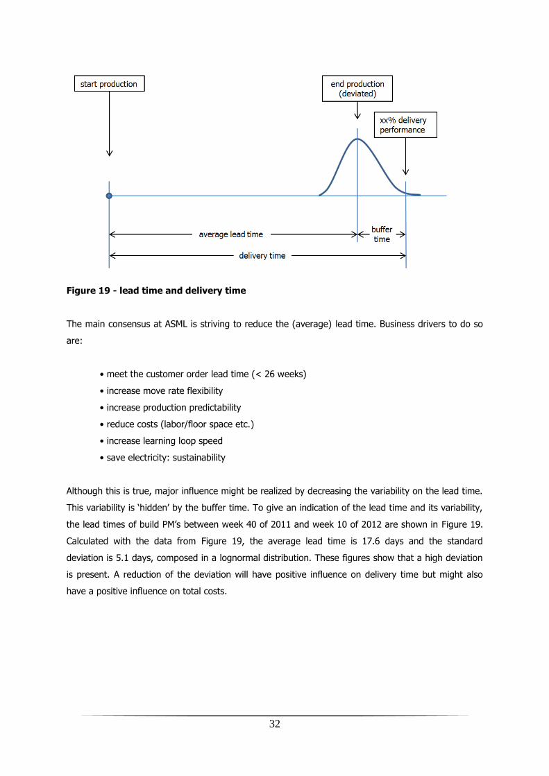
Figure 19 - lead time and delivery time

The main consensus at ASML is striving to reduce the (average) lead time. Business drivers to do so

are:

• meet the customer order lead time (< 26 weeks)

• increase move rate flexibility

• increase production predictability

• reduce costs (labor/floor space etc.)

• increase learning loop speed

• save electricity: sustainability

Although this is true, major influence might be realized by decreasing the variability on the lead time.

This variability is „hidden‟ by the buffer time. To give an indication of the lead time and its variability,

the lead times of build PM‟s between week 40 of 2011 and week 10 of 2012 are shown in Figure 19.

Calculated with the data from Figure 19, the average lead time is 17.6 days and the standard

deviation is 5.1 days, composed in a lognormal distribution. These figures show that a high deviation

is present. A reduction of the deviation will have positive influence on delivery time but might also

have a positive influence on total costs.

33

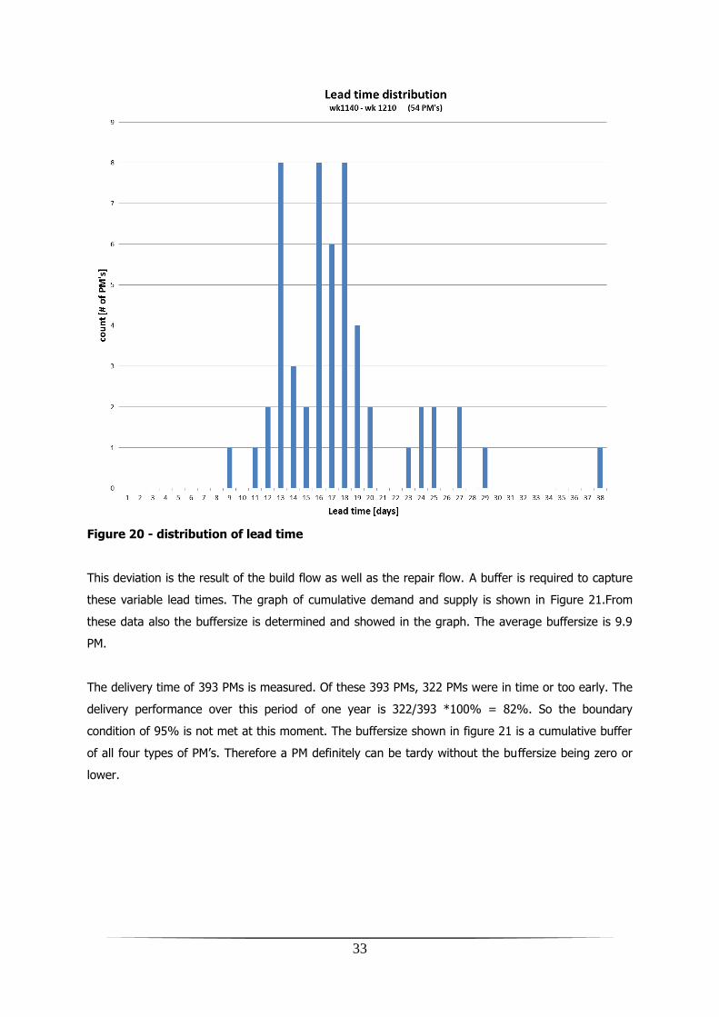
Figure 20 - distribution of lead time

This deviation is the result of the build flow as well as the repair flow. A buffer is required to capture

these variable lead times. The graph of cumulative demand and supply is shown in Figure 21.From

these data also the buffersize is determined and showed in the graph. The average buffersize is 9.9

PM.

The delivery time of 393 PMs is measured. Of these 393 PMs, 322 PMs were in time or too early. The

delivery performance over this period of one year is 322/393 *100% = 82%. So the boundary

condition of 95% is not met at this moment. The buffersize shown in figure 21 is a cumulative buffer

of all four types of PM‟s. Therefore a PM definitely can be tardy without the buffersize being zero or

lower.

34

Figure 21 - Cumulative supply and demand

View Figure 21. In a situation without repair, a certain buffersize is required to capture the

differences between supply moments and demand moments. When a PM is rejected from testrig or

test, two events take place. First, the rejected PM is waiting to be repaired. It is added to the

production system and therefore requires a part of the capacity. Second, an immediate order for

another PM is created. The demand moment is equal to the moment the reject took place. To fulfill

this demand, a PM from the buffer is consumed. This creates the situation of a lower buffer for the

time being the rejected PM is repaired. This buffer is used to cover variability‟s but does not take into

account the variability‟s due to sudden demands created by rejected PM‟s. This partially results in

lower than required delivery performance. Three directions to solve this problem are possible:

1. Take into account the variability of rejected PM‟s by increasing the buffer.

2. Reduce the lead-time of the repair PM‟s.

3. Change from piece-buffer to time-buffer per produced PM in order to gain control over the

composition of the buffer.

Taking into account the costs parameter makes it possible to make choices regarding these

measurements in order to either meet the required delivery performance and to meet it against the

lowest possible costs.

35

Figure 22 - Schematic view (1)

5.4. Indistinct handling of rejected PM’s It is noticed that there is no strict procedure to reject a PM from testrig or test and return it back to

the PM workcenter to repair it. When a PM is rejected from testrig or test, it is unclear how to deal

with the rejected PM and bring it to the PM workcenter. The process is unstandardized and fulfilled in

different ways. There is often a lack of specific data of the repaired PM this and leads to confusion

and unnecessary communication between the stakeholders. Rejected PM‟s are buffered. Subsequently

several actions needs to be performed in order to create the right information at the right place. The

problem in here is that there is no knowledge of which information has to be handed over and in

which sequence the stakeholders need to perform their action to provide this information.

In [in „t Veld, 2002]an explanation is given about data types and data flows. The goal of data is to

provide multiple functions in the organization of the right information, which will be used in these

functions for decision-making. Awareness of the different data types is important because of:

T = 0

T = 1

repair

PM

order

repair

PM

PM

PM

PM

PMPM

PM

order

3

PM PM

order

2

order

1

PM

order

3

PM PM

order

2

order

1

Size = n

Size = n - 1

?

repair repaired PMrejected PM

Figure 23-Flow of rejected PMs

36

creation of systematic data needs.

coherence of these data needs between the organs of an organization.

Possibilities to a fit of the applied organizational structure.

[In „t Veld, 2002] first distinguishes data types in several aspects. After that, he raises questions

which must be able to become answered when applying data handling in a certain production system,

for example a steady state production line, like the PM production of ASML.

There is a difference in data types between the data needed to be able to produce the product and

data which are required to be able to control the production process. Data needed to be able to

produce the product is separated in product-identity data and data committed to the production

location. Regarding the rejected PM flow, the data committed to the production location can be left

out of consideration, since it is clear that this problem is about product specific data of the rejected

PM.

Furthermore, when designing a process in which these data is processed, one must take into account

if the right data is given by the right entity at the right time and enters the right location in the right

configuration. By designing this process, questions raise like:

Which data needs to be:

o Imported?

o Exported?

o Buffered?

Where does these data come from?

Which actions need to be taken in which sequence to supply the data?

Where must the data be send to, in which combination and in what configuration?

[In „t veld, 2002] explains data handling in three steady state types: the process line, the functional

structure and the grouped production. Although none of this is the situation of this problem, it

becomes clear that a correct data handling can be realized in two steps:

First: investigate and mark the types of required data.

Second: Develop a process which prescribes the providing of the required data by the stakeholders in

the right sequence.

5.5. Conclusion The „assemble PM‟-function consists of two stages regarding the regular PM flow. First the

subassemblies are built. Then the subassemblies are integrated to a PM. Rejected PM‟s are analyzed

37

and dismounted. About one third of the rejected PM‟s consists of quick fix PM‟s. From the rejected

PM‟s which are considered as regular repair PM‟s, the possibilities of the occurrence of subassemblies

to be repaired are calculated.

To fulfill the demand created by rejected PM‟s a PM from the buffer is consumed. This creates the

situation of a lower buffer for the time being the rejected PM is repaired. This buffer is used to cover

variability but does not take into account the variability due to sudden demands created by rejected

PM‟s. This partially results in lower than required delivery performance. Two directions to solve this

problem are possible:

1. Take into account the variability of rejected PM‟s by increasing the buffer.

2. Reduce the lead-time of the repair PM‟s.

3. Change from piece-buffer to time-buffer per produced PM in order to gain control over the

composition of the buffer.

There is no strict procedure to reject a PM from testrig or test and return it back to the PM

workcenter to repair it. When a PM is rejected from testrig or test, it is unclear how to deal with the

rejected PM and bring it to the PM workcenter. The process is unstandardized and fulfilled in different

ways. There is often a lack of specific data of the repaired PM this and leads to confusion and

unnecessary communication between the stakeholders.

38

39

6. Production structure of ‘Assemble PM’

6.1. Functional structure A zoom in the functions „build‟ and „integrate‟ of Figure 15 is visualized. The structure of the „build‟

process consists of five processes, each dedicated to one subassembly. The hose assy is integrated to

the carrier base already before delivering the carrier base to the integration section. Three other

subassemblies remain; the crash rim, the short stroke motor and the chuck assy. The subassy‟s to be

repaired are added to the relevant process as well. Percentage of occurrence is already shown in

Table 5.

Figure 24 - zoom into 'build'

A zoom in the „integrate‟ process is shown in Figure 25. One notices multiple integration steps. First

the integration of the carrier base with the crash rim, short stroke motor and LOS motor (supplier

part) takes place. Then this „bottom PM‟ is tested on PMQT1. After that, the integration of the top

part, the chuck assy with the bottom part takes place. PMQT2 takes place and after that, some

finalize operations do have to be executed. Repair PM‟s are added on both integration operations, but

mainly to the first operation. 4% of the PM‟s do only advance the second integration operation and

the PMQT2 operation.

integrate

assemble

carrier

base

hose

assy

assemble crash rim

assemble chuck assy

assemble SS motor

hose

assy

repair sub-assy

40

Figure 25 - zoom into 'integrate'

6.2. Production structure In [In„t Veld, 1999] production structures are explained. In this paragraph the appropriate structure

for the „assemble PM‟-function is defined by means of the literature of In ‟t Veld. In‟t Veld discusses

two kinds of structures; the flow oriented structure and the functional structure. The production and

reparation of the PM‟s is executed in a flow oriented structure.

Before assessing the appropriate structure of the reparation of the PM‟s, first the situation at AM-WSN

is described. The production and reparation of the PM‟s is subject to a lot of disturbances. Due to

these disturbances, the lead times are differing. To accommodate the deviations in lead time, buffer

time is necessary. The labor consists largely of the assembling of materials and qualifying the PM.

Automation is not possible, since the production and reparation of the PM‟s takes place in

cleanrooms. These are clean environments in which pollution (f.e. from rotating parts of production

machines) must be strictly avoided. Thereby, the PM‟s require manual labor due to the small size of

the materials, the precision of execution of the assembling operations, the relatively low production

numbers and the constantly changing design. Currently, the workstations meet high process times

per order. The typical time required of a PM being at one workstation differs from half a day up to 3

days.

The flow oriented structure has been distinguished to subgroups by In „t Veld. Following

[organisatiestructuur en arbeidsplaats,figure 6.4], In „t Veld starts discussing the continuous process

production and following the intermittent line production. Since ASML faces a lot of disturbances

during the PM production and reparation, this will not be the appropriate structure. Subsequently, a

division is made into structures facing long station times and structures facing short station times.

The choice for a structure which deals with long station times is clear, since this is the case in the

production process of the PM‟s.

Due to the long station times, there‟s chosen to design the PM with a modular structure. The PM

consists of five sub modules. Each of them is produced on separate workstations. This measurement

finalizeTest

(PMQT1)integrate

test

(PMQT2)integrate PM

carrier

base

cra

sh r

im

SS

moto

r

LO

S m

oto

rs

chuck a

ssy

repair PM repair PM

41

already may have led to a reduction of the amount of disturbances due to the repeating work.

Although sub modules are already introduced, the integration and qualification of these sub modules

to one PM still requires long station times. The effect of long station times is reduced by using a

mixed model line. There are four types of PM‟s processed in the workcenter, the PM311LEX,

PM311REX, PM321LEX and the PM321REX. The station times thereby are considered as acceptable.

The integration and qualification process currently has a streetwise structure. The assembling of the

submodules is executed in groups also. The group-technology used for the sub modules is the cell-

layout.

Reasons to implement group-layout in a production process are as follows [P. van Amelsvoort, 1988]:

Increase of flexibility

Reduction of throughput times

Reduction of transport and storage

Increase of awareness for quality by the operators

Increase of delivery performance

Increase of attractiveness of the labor

Simplified process control

After discussions (program managers, output leaders) it becomes clear that ASML considers it very

important to have dedicated and committed operators. Due to the complexity of the product and the

high influences of the assembly operations, the dedication of the operator is an important factor on

the quality of the product. As mentioned by [P. van Amelsvoort, 1988] an important reason for group

technology is the increase of awareness for quality by the operators. This is the main reason for ASML

to use group-layout, and, referring to the literature, it is a legitimate one. Nevertheless, also the other

reasons described by [P. van Amelsvoort, 1988] to apply group layout do bring its advantages to the

production of ASML. It can be concluded that the group technology as currently applied in the

„assemble PM‟-function is an appropriate production structure for the production of the PM.

6.3. Capacity

6.3.1. Workstations

In this section the number of workstations and its capacity will be evaluated. Every process is

executed on one of a dedicated group of workstations. The short stroke process has been divided into

two sequential processes, first the assembling of the short stroke and then the SSMQ (the quality test

of the short stroke).

The integrate process of the PM is more complex. The integration of the short stroke onto the carrier

base requires a dedicated and expensive tool (shimming tool). For that reason this integration

42

process is divided into three sequential operations. First the shimming tool is used(integration SS),

then the LOS motors are assembled (integration LOS) on a separate workstation and then the PM

passes the shimming tool again to fulfill the „INT CB+SS+CR+LOS‟ process. After that, the PMQT1

test follows on a PMQT tool. PMQT tools are used for both PMQT1 and PMQT2 tests.

The number of workstations and the calculated capacity of number of PM‟s per week are showed in

Table 6.The workcontent is based on a-time, b-chance and average b-duration of the tables of

appendix J.An extensive explanation of these time-types, the handling of disturbances and

quantification can be found in appendix F. The average workcontent per PM is determined by adding

the workcontent of all n operation steps [x] per workstation, which leads to the following calculation:

[𝐸𝑞. 6.1] 𝑤𝑜𝑟𝑘𝑐𝑜𝑛𝑡𝑒𝑛𝑡𝑎𝑣𝑒𝑟𝑎𝑔𝑒 = (𝐴𝑡𝑖𝑚𝑒 + 𝐵𝑐𝑕𝑎𝑛𝑐𝑒 ∗ 𝐵𝑑𝑢𝑟𝑎𝑡𝑖𝑜𝑛𝑎𝑣𝑒𝑟𝑎 𝑔𝑒 )

𝑛

𝑥=1

The B-distribution per operation step is specified according to the method explained in appendix G.

An average B-duration follows out of this B-distribution.

Table 6– Workstationgroups and its capacities

As can be seen, the bottleneck is the „integration SS‟ workstation, since this workstation has the

lowest capacity (13.7 PM/w). It is required to obtain a moverate of 11 PM/week. According to the

capacity of the workstations it must be possible to achieve this. The aspect of high variability due to

disturbances and rejected PM‟s is not taken into account. Measured over a long period of time, this

will not influence the obtained moverate but does have its influence on lead time and delivery

performance. To investigate the effect of the variability‟s on the performance of the production

system, a simulation is required.

type of workstation # workcontent/PM [h] max. capacity [PM/w]

hose assy 2 12.2 13.8

carrier base 4 21.4 15.7

crash rim 2 10.4 16.2

ss motor 5 22.5 18.7

SSMQ 2 11.3 14.9

chuck assy 3 9.0 28.0

integration SS 4 24.6 13.7

integration LOS 2 10.9 15.4

PMQT 4 18.6 18.1

integration CA 3 9.3 27.1

finalize 4 14.8 22.7

43

6.3.2. Operators

The second capacity aspect expresses itself in manpower. For the building of the subassemblies and

the integration of these assemblies to a complete and tested PM, there are four operation teams

available. Two teams are assigned to build the subassemblies; the other two teams integrate and test

the PMs. The teams substitute each other in morning and evening shifts. Together a week schedule

of 12 shifts per week is fulfilled. During office days two shifts per day is performed. On weekend

days, only one shift per day. This leads to a total of 12 shifts per week. The effective available hours

per shift is indicated in Figure 26. As shown, the operators are present for the time of 9 hours per

shift. With subtraction of the breaks and the shift transfer, only 7 hours per shift is left. This results in

an effective available amount of working time of 84 hours/week.

Figure 26- Shift breakdown

In appendix E the effective available labor-hours per week is shown over a period of 36 weeks. The

size of the operator-teams per shift can be calculated using the data of this table. It follows that the

average amount of effective available labor-hours per week of the „build‟-function (subassy) is 1024

hours. This is equal to an available number of operators of 1024/84=12.2 operators. The average

amount of effective available labor-hours per week of the „integrate‟-function is 867 hours. This

results in an available number of operators of 867/84=10.4 operators.

What is the capacity (in terms of number of PM‟s per week) of the operators? To answer this

question, it is necessary to calculate the total amount of labor required for one (regular build) PM,

including the (possible) repair operations. With the data of Table 2, Table 3, Table 5 and appendix J

respectively the yield loss is known, the percentages of quick fix repairs is known, the chances on the

different kinds of subassy repair is known and the workcontent per process is known. Out of these

44

data, the part of the workcontent of regular operations as well as repair-operations per regular build

PM is calculated. In the second column of this table the regular workcontent per process type is

shown. In total an average of 86.8 hours is required to fulfill the subassy processes for one regular

PM. Per regular PM on average also 6.7 hours is spend to reparation of subassemblies. In total 93.5

hours are required for subassy fulfillment or one regular PM. For the integration of the PM, 78.2 hours

is required per regular PM. Another 29.8 hours on average is required to fulfill the reparation of a

regular PM. In total 108 hours on average is required for the integration process of one regular PM.

Table 7 - Workcontent per regular PM

The total available labor-hours per week divided by the total average workcontent per regular PM

results in a maximum capacity of 10.8 regular build PM‟s per week for the subassy operator teams

and 8.6 regular build PM‟s per week for the integration operator teams. Using the yield loss as

defined before (32%), the maximum capacity for subassy is 15.9 PM‟s per week. The maximum

capacity for integration is 12.6 PM‟s per week. Of both the „workstation‟ resources and the

„manpower‟ resources, the integration operators do currently have the lowest capacity (highest

occupancy rate) and will therefore be the bottleneck of the „assemble PM‟-function.

Table 8 - Maximum capacity of operator teams

6.4. Effect of the repair flow From Figure 13 the question raised whether the repair PM‟s do negatively affect the output of regular

PM‟s of the workcenter or not.

type of process workcontent/buildPM [h] repaircontent/buildPM [h] total [h]

hose assy 12.2 0.2 12.4

carrier base 21.4 0.6 22.0

crash rim 10.4 0.8 11.2

ss motor 22.5 3.1 25.6

SSMQ 11.3 1.5 12.8

chuck assy 9.0 0.5 9.5

subassy total 86.8 6.7 93.5

integration 78.2 23.9 102.1

quickfix 0.0 5.8 5.8

integration total 78.2 29.8 108.0

operatorteamtotal average

content/buildPM [h]

# of

operators

total available

manpower [h/week]

max # build-

PM's/week

max #

PM's/week

sub assy 93.5 12 1008 10.8 15.9

integration 108.0 11 924 8.6 12.6

45

Figure 27 - Buffer size

Figure 28- Rejected PM's

The pattern of the origination of rejected PM‟s is plotted in the time. This is shown in Figure 28. As

one notice, there are two periods in which an above average number of rejected PM‟s arise during a

few consecutive weeks. As is known from Figure 27 also two periods of delivery problems occurred.

These are marked in Figure 28 by the black ellipses. It becomes clear that these periods do have

negative influence on the delivery performance. This phenomenon is explained by means of the

schematic view of Figure 29.

When an above average number of PM‟s is rejected during multiple weeks, the effect explained in

Figure 22 becomes amplified. The demand caused by the rejected PM‟s consumes the buffered PM‟s.

When the production system would cope with the temporary higher required capacity, the buffer

would be filled reasonably on time. But due to the combination of the above average number of

rejected PM‟s and a limited capacity, the end buffer decreases in size. From that moment on, the

supply of the PM‟s suffer by a delay and the delivery performance will decrease. The situation turns to

normal when the buffer at the outbound side is filled again. This phenomenon does have a negative

influence on the delivery performance. Research by simulation would indicate whether the current

capacity is appropriate to handle the severe demand and supply fluctuations.

0

2

4

6

8

10

12

14

16

11

36

11

37

11

38

11

39

11

40

11

41

11

42

11

43

11

44

11

45

11

46

11

47

11

48

11

49

11

50

11

51

11

52

12

01

12

02

12

03

12

04

12

05

12

06

12

07

12

08

12

09

12

10

12

11

12

12

12

13

12

14

12

15

12

16

12

17

12

18

12

19

12

20

12

21

12

22

12

23

12

24

12

25

12

26

12

27

12

28

12

29

12

30

12

31

Bu

ffe

rsiz

e [

# P

M's

]

Week

Mk311

Mk321

0

1

2

3

4

5

6

7

8

# PM

Week

Rejected PM's

testrig

test

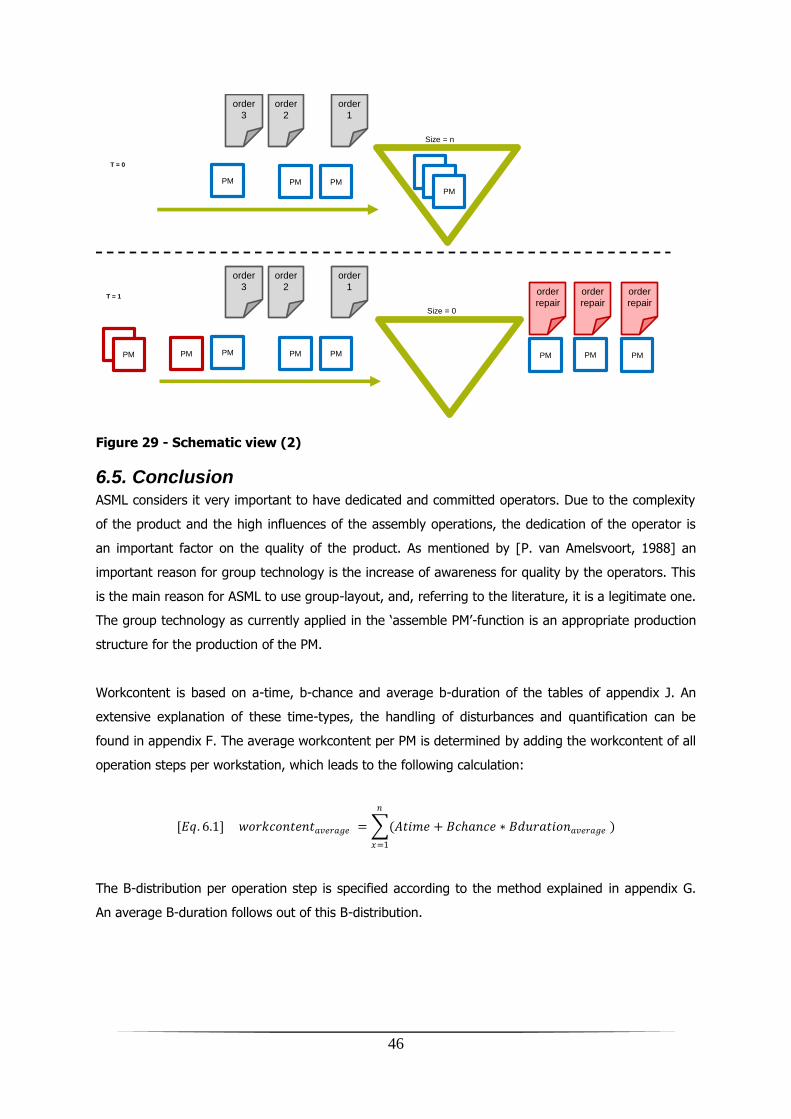
46

Figure 29 - Schematic view (2)

6.5. Conclusion ASML considers it very important to have dedicated and committed operators. Due to the complexity

of the product and the high influences of the assembly operations, the dedication of the operator is

an important factor on the quality of the product. As mentioned by [P. van Amelsvoort, 1988] an

important reason for group technology is the increase of awareness for quality by the operators. This

is the main reason for ASML to use group-layout, and, referring to the literature, it is a legitimate one.

The group technology as currently applied in the „assemble PM‟-function is an appropriate production

structure for the production of the PM.

Workcontent is based on a-time, b-chance and average b-duration of the tables of appendix J. An

extensive explanation of these time-types, the handling of disturbances and quantification can be

found in appendix F. The average workcontent per PM is determined by adding the workcontent of all

operation steps per workstation, which leads to the following calculation:

[𝐸𝑞. 6.1] 𝑤𝑜𝑟𝑘𝑐𝑜𝑛𝑡𝑒𝑛𝑡𝑎𝑣𝑒𝑟𝑎𝑔𝑒 = (𝐴𝑡𝑖𝑚𝑒 + 𝐵𝑐𝑕𝑎𝑛𝑐𝑒 ∗ 𝐵𝑑𝑢𝑟𝑎𝑡𝑖𝑜𝑛𝑎𝑣𝑒𝑟𝑎𝑔𝑒 )

𝑛

𝑥=1

The B-distribution per operation step is specified according to the method explained in appendix G.

An average B-duration follows out of this B-distribution.

T = 0

PM

order

3

PM PM

order

2

order

1

T = 1

PM

order

repair

PM

PM

PM

PM PM PM

order

repair

order

repair

PM

order

3

PM PM

order

2

order

1

PM

PM

Size = n

Size = 0

47

As can be seen in Table 6, the bottleneck is the „integration SS‟ workstation, since this workstation

contains the lowest capacity (13.7 PM/w). It is required to obtain a moverate of 11 PM/week.

According to the capacity of the workstations it must be possible to achieve this.

The maximum capacity of the integration operator team is 12.6 PM‟s per week. Of both the

„workstation‟ resources and the „manpower‟ resources, the integration operators do currently have the

lowest capacity (highest occupancy rate) and will therefore be the bottleneck of the „assemble PM‟-

function.

Delivery performance suffers when an above average number of PM‟s is rejected during multiple

weeks. Due to the combination of the above average number of rejected PM‟s and a limited capacity,

the outbound buffer decreases in size. From that moment on, the supply of the PM‟s suffer by a delay

and the delivery performance will decrease. Research by simulation would indicate whether the

current capacity is appropriate to handle the severe demand and supply fluctuations.

48

49

7. Problem statement The requirements as stated in the introduction section are repeated:




The problems found are described below:

1. Indistinct reject trajectory

There is no strict procedure to reject a PM from testrig or test and return it back to the PM

workcenter to repair it. When a PM is rejected from testrig or test, it is unclear how to deal with the

rejected PM. The process is unstandardized, based on mouth-to-mouth, singular appointments and is

fulfilled in different ways. There is often a lack of specific data of the repaired PM and this leads to

confusion and unnecessary communication between the stakeholders.

2. Low delivery performance

Currently the production system doesn‟t meet its requirements. The moverate is met, but the

delivery performance is equal to 82% and therefore it is lower than the required delivery

performance of 95%.The problems described below are cause-related to the unfulfilled

delivery performance requirement.

a. Low buffersize: To fulfill the demand created by rejected PM‟s a PM from the buffer

is consumed. This creates the situation of a lower buffer for the time being the

rejected PM is repaired. This buffer is used to cover variability but is temporary too

low to meet the delivery performance requirement.

b. Wrong composition of buffer: The buffer is not controlled and is currently filled

by producing PM‟s without demand. Therefore it is unclear what the optimal

composition is.

c. Long repair lead-time: The buffer is lower for the time being a rejected PM is

repaired. A long repair lead-time therefore has a negative influence on the delivery

performance.

d. Capacity shortage: Delivery performance suffers when an above average number

of PM‟s is rejected during multiple weeks. Due to the combination of the above

average number of rejected PM‟s and a limited capacity, the buffer at the outbound

side of the production system empties. The supply of the PM‟s suffers by a delay and

the delivery performance will decrease. Research by simulation would indicate

whether the current capacity is appropriate to handle the severe demand and supply

fluctuations.

50

3. Unknown economic value of yield improvement

A yield loss of 32% is undesirable high. ASML aims to reduce the yield loss to 12%. However, the


51

III. Solution

52

53

8. Solution directions As a result of the analysis part, three problems are stipulated. These problems need to be solved by

solid solutions. In this chapter the solution directions are described.

8.1. Solution method The first problem is handled in chapter 9. First an introduction to the problem is given. Then the

processes are explained and solutions are determined. Finally the execution is explained, where the

standardized process and a dashboard are shown.

For the second and third problem it is chosen to use the Tecnomatix® plant simulation package of

SIEMENS PLM Software. It is unclear in which degree the high fluctuations in the pattern of rejected

PM‟s influence the performance of the production system. Calculations by hand could provide a lot of

information regarding the performance of this workcenter, but only with simulation it is possible to

take fluctuations into account. Especially the high fluctuations this production system has to deal

with, makes simulation the right choice to found improvement decisions.

Chapter 10 shows the design of the simulation model in process description language. In chapter 11

the simulation model is verified and validated. A confidence analysis of all experiments is executed

and explained in chapter 12. Chapter 13 finally shows the analysis of the results of the executed

experiments and a sensitivity analysis.

8.2. Experimental design Regarding simulation, experiments can be designed in multiple ways. Three common experimental

design methods are:

• Rule base

• Genetic algorithm

• Multi-level

A genetic algorithm is especially useful when the solution space do contain multiple local optima. A

disadvantage of GA is that although it gives the global optimum, it is unclear how the solution space

looks like. This also counts for the rule-base method. A multi-level experimental design gives clear

insight in the shape of the solution space, but will take a long execution time. Due to the importance

of understanding the solution space, it is chosen to use a multi-level experimental design.

The three subproblems of problem 2 can be divided into two parts. The first part exists of subproblem

b and c. These problems indicate respectively to reduce the repair lead time and to increase the

capacity. Both of these measurements lead to differing properties of the actual production process

54

itself. Opposite, a change of the endbuffersize (problem 2.a) does not influence the properties of the

production process. Therefore, first the approaches regarding problems 2.b and 2.c are explained.

Problem 2.b (long repair lead time), is explored by separating the regular build flow from the repair

flow. The repair flow will use flexible workstations. These workstations will be able to execute all

integration operations with exception of the PMQT operations. The PMQT stations are dedicated test

stations and therefore cannot be integrated to a flexible workstation. It is assumed that separation of

the flows lead to a decreased repair lead time. This will result to a faster restoration of the end buffer

and therefore to a lower required end buffer size. On the other hand, the assignment of resources

will be more inflexible. This trade-off will be quantified by means of the simulation model.

Problem 2.c (capacity shortage) is investigated by altering the both resource types. Of both the

subassy operators as the integration operators, the integration operators do have to deal with the

highest occupancy rate. Therefore, in every executed scenario, the number of integration operators is

changed. In the case of the separated flows, the integration team for regular PM‟s is smaller,

dependent on the amount of repair operators. In this way, the number of operators is equally altered

in every scenario. Also the workstation resource type is altered. In this case, the bottleneck

workstation („integrate SS‟ workstation, which is a shimming tool) will be increased with one, to five

workstations.

The scenarios are shown in the matrix of Table 9. This shows that there are four scenarios. In the

case of scenario 3 and scenario 4, in order to equalize the number of workstations with scenario 1

and scenario 2 respectively, one workstation of the chuck assy process, one workstation of the

integrate CA process and one shimming tool is removed. These workstations are selected to realize a

bottleneck with the lowest occupancy rate possible.

Table 9 - Scenarios

Problem 2.a (low endbuffersize) is solved by increasing the endbuffersize. This can be realized in

different manners. First, the changes in the process itself, for example the scenario‟s described

above, do influence the required endbuffersize. Furthermore, the endbuffersize can be increased by

earlier starting the regular build PM‟s or by producing a certain number of PM‟s without demand. The

# current mixed flow separated flow

current # of workstationsscenario 1:

4 shim. tools

scenario 3:

3 repair stations

# of workstations + 1scenario 2:

5 shim. tools

scenario 4:

4 repair stations

55

production of PM‟s without demand gives two input parameters (start moment and # of PM‟s

produced for buffer) for one output parameter (buffersize). Because of the predefined production

quantities due to the moverate, it is known well in advance which type of PM needs to be started on

what moment. Therefore the start moment is used to change the endbuffersize. This start moment is

altered from 18 to 32 days before the demand date. As described above, also the integration operator

team is altered. This leads to a matrix of 90 experiments to be executed for every scenario. This is

shown in Table 10.

Table 10 - Experimental design

All experiment results are measured based on the total costs per PM, which is the result of the cost

function described in chapter 10. The second key performance parameter is the delivery performance.

Moverate is determined to be constant.

Problem 3 is investigated by executing the current scenario (scenario 1) with different yield losses.

Again the performances are given in terms of total variable costs and delivery performance. By

comparing the costs with equal delivery performance, the economic value of a yield improvement can

be calculated.

Table 11 - Yield loss experiments

10 11 12 13 14 15

18 . . . . . .

19 . . . . . .

20 . . . . . .

21 . . . . . .

22 . . . . . .

23 . . . . . .

24 . . . . . .

25 . . . . . .

26 . . . . . .

27 . . . . . .

28 . . . . . .

29 . . . . . .

30 . . . . . .

31 . . . . . .

32 . . . . . .

start momentintegration operators

# AS-IS yield levelAimed yield

level

Maximum

yield level

Scenarioscenario 1:

yield 68%

scenario 1:

yield 88%

scenario 1:

yield 100%

56

57

9. Qualitative feed forward control for rejected PM’s

9.1. Introduction It is noticed that there is no strict procedure to reject a PM from testrig or test and return it back to

the PM workcenter to repair it. When a PM is rejected from testrig or test, it is unclear how to deal

with the rejected PM and bring it to the PM workcenter. The process is unstandardized, based on

mouth-to-mouth, singular appointments and is fulfilled in different ways. There is often a lack of

specific data of the repaired PM this and leads to confusion and unnecessary communication between

the stakeholders. The problem in here is that there is no knowledge of which information has to be

handed over and in which sequence the stakeholders need to perform their action to provide this

information.

In two steps the current problem of indistinct rejection procedures can be solved. First it is stipulated

which information is required to fulfill the rejection of PM‟s in a standardized manner. Second, the

actual standardization of the process follows.

The advantages of clarifying the required information and standardizing the process are the following:

Every stakeholder will be able to access the correct and complete information

required.

The correct registration will bring benefits in analysis of process and product.

Smoothing the process will reduce the presence-time of rejected PM‟s in the

workcenter.

9.2. Solution Through the whole process of „PM to be rejected‟ up to the moment the repaired PM is added to the

end buffer on multiple moments information is required before it is possible to proceed to the next

process. At these locations, control loops have to be added to the process. In the following section,

the whole process is explained step-by-step, the required changes are stipulated and the kinds of

information are described.

?

repair repaired PMrejected PM

Figure 30-flow of rejected PMs

58

The whole cycle of a PM to be rejected until the moment it is repaired again can be divided into four

main processes:

1. Escalation

2. Rejection

3. Analysis

4. Repair

Escalation

Every process is thoroughly explained. First the PM is situated at a lithography machine or testrig.

Just as is described in appendix E a disturbance notification occurs due to a problem. After the

regular escalation to the first, second and finally the third line support, a decision is made whether

the disturbance will be resolved locally or the disturbance is severe enough to reject the PM. These

decisions are made by the third line support (D&E).

Rejection

When it is decided to reject the PM, three process steps needs to be executed. The PM needs to

become drained. This is executed by the Machine father. After that, a support team of AM-WSN is

formed to remove the PM and transfer it back to the workcenter. While the first step (drain) just

requires operators which are already present at the machine, the second and third step are executed

by the second line support of AM-WSN (TOPS). Therefore it is important that the stakeholders from

AM-WSN do get access to the right information.

Figure 31 - Reject process

The machine father has to create a support request for AM-WSN. This request is handled by one of

the TOPS team leaders of AM-WSN. The team leader follows by giving permission to start the removal

of the PM from the machine or testrig. The control is executed by the TOPS team leader. The

positioning of the control loop is shown in Figure 32.

reject rejected PMPM to be rejected

rejected PMPM to be rejected drain remove transfer

59

Figure 32 - Control over the reject process

Analysis

After the PM is rejected and transferred to the AM-WSN workcenter, the PM is buffered in order to

acquire the correct information before the reparation is started. The analysis and repair process are

currently not separated. This gives an incomplete and confusing view on the progress of rejected

PM‟s. Besides, information is created during analysis on behalf of the repair process. Separation of

these processes and design dedicated control of both of the processes will contribute to distinction of

the overall process.

Figure 33 - Control over the analyze/repair process

The machine father creates a material notification (MN) and registers the following info in the MN:

PM equipment #

Module #

DN # on machine

Summary of issue/suspected cause of failure

AIR ID

The machine father also creates a task for the material handler to order a new PM for the lithography

machine or testrig. The material handler creates a task for Production planning to allocate a PM. This

allocation will be one of these two directions:

control

standards

PM to be rejected drain remove

repair repaired PManalyzerejected PM

controlcontrol

standards standards

60

1. The rejected PM is considered to be a quick fix and returns in the same testrig/test sequence.

2. The rejected PM is swapped by another PM from stock.

A trade-off is made by production planning based on the progress of the sequence of the rejected

PM, the severity of the disturbance of the rejected PM and the possibilities to offer a PM from stock.

Production planning also creates an analysis order. After the creation of the analysis order, the

material notification created by the machine father is added to the analysis order. All PM specific

information regarding the repair process is saved into this material notification.

Concurrently, Manufacturing Engineering (ME) has to provide an action plan. This action plan is based

on archived information available at the ME department and PM specific information. This PM specific

information is gathered during the escalation process on the lithography machine. The action plan is

checked by TOPS before the start of the analysis. TOPS gives its approval for the action plan when it

is clear which steps to execute. After that, the action plan is added to the material notification by

TOPS.

Summarized, the following information carrier‟s needs to be present before start of the analysis of the

rejected PM may take place.

Table 12 - Information and stakeholders (1)

Repair

After analysis of the rejected PM, TOPS must be able to confirm the causes stipulated by

manufacturing engineering. Based on the new information, it is known which repair actions needs to

be executed. Production planning creates a repair order. TOPS performs a material request when

necessary. The material request is treated by material handling, which orders material. The repair

order contains a standard routing. TOPS creates additional routings in the repair order and changes

the standard routings when necessary. When these steps are fulfilled, the operator can start the

reparation.

information responsible stakeholder

analysis order available Production planning & control

material notification available machine father

MN added to analysis order machine father

action plan available ME-test & ME-WSN

action plan approved TOPS

action plan added to MN TOPS

61

Table 13 - Information and stakeholders (2)

9.3. Execution Both the process described above and the required information is consolidated. An overview of the

swimming lane process is given in appendix B. Every step described above is present in the swimming

lane model. Also the information is controlled by a dashboard. This is shown in appendix C. It

resulted in a clear overview of the progress of every rejected PM. The columns indicate which

information is required. The rows do show the PM‟s and the cells give information whether the

relevant step of a certain PM is already executed or not.

information responsible stakeholder

material request performed? TOPS

material ordered? MH

additional routings required? TOPS

routings added (if necessary) and edited? Means & Methods

62

63

10. Simulation model

10.1. Introduction Simulations runs equals the period of one year, with a ramp-up of 100 days. This is defined in

appendix H. The simulation model is designed by the descriptions given below:

1) There‟s a set of workstationgroups containing workstations of the same kind.

2) PM-orders contain suborders.

3) Suborders, containing an assemblyplan are executed on a workstation of a workstationgroup.

4) Every workstation in the same workstationgroup contains the same set of assemblyplans.

5) The assemblyplans contain a table with several sequential operation steps and information

regarding a-times, b-chances, b-duration, successors, required service, etc.

6) Every operation step has its own process time. This process time is defined out of the input

given for this process step from the table.

7) The routing of PM-orders for build PM‟s is identical for each order. The routing of PM-orders

between the workstationgroups for repair PM‟s may vary for each PM-order.

8) PM orders of regular PM‟s are created with an interval based on a negative exponential

distribution. Further explanation follows in appendix I.

Figure 34 - Assemblyplan

Figure 35 - PM order, suborder and WorkstationGroup

64

Figure 36 - Schematic view of PM flow

65

10.2. Process description language

Definition section

Ordersource

- NewPMorder

- Newsuborder

Process: Method

WorkstationGroup

- WorkstationQ

- IdleQ

- SuborderQ

- MyAssemblyPlans

- SelectPMorder: Method

Workstation

- MyGroup

- MySuborder

Process: Method

Assemblyplan

- MyGroup

- MyTable

EndBuffer

- EndBufferQ

- Duedatelist

Orderdrain

- Newrepairorder

Process: Method

Repairdistributor

- Repairchancestable

- MyPMorder

Process: Method

PMorder

- Label

- startdate

- suborderlist

- leadtime

- buffertime

- deliverytime

- repairchance

- quickfix :boolean

Suborder

- MyPMorder

- MyAssemblyPlan

66

Process section

Ordersource.process

Repeat

Advance(Sample(interarrivaltime))

NewPMorder = PMorder.create

NewPMorder.suborderlist.create

x=1

Repeat(number of suborders)

x = x+1

NewSubOrder = Suborder.create

NewSubOrder.OnGroup = (‘WorkstationGroup x’)

Select [WorkstationGroup x].Assemblyplan //based on type of PM-order

NewPMorder.startdate = TNow

Add NewPMorder.label to Duedatelist

Add (NewPMorder.startdate + normCT) to NewPMorder.label on Duedatelist

NewPMorder.orderlist.first.Enter(NewPMorder.suborderlist.first.OnGroup.suborderQ)

Workstation.process

Repeat

Enter(IdleQ)

While MyGroup.suborderQ.IsEmpty do standby

Leave(IdleQ)

Mysuborder = MyGroup.Selectsuborder

MyAssemblyPlan = Mysuborder.MyAssemblyPlan

MyGroup.suborderQ.Remove(MySuborder)

Repeat(MyAssemblyPlan.Mytable.length)

If MyAssemblyplan.Mytable.Operation.Materials <> Nil then

If Materials.IsInQueue(StorageArea) then StorageArea.Remove(.Materials)

If MyAssemblyplan.Mytable.Operation.Resources <> Nil then

IfResources.IsInQueue(IdleOperatorQ) thenIdleOperatorQ.Remove(Resources)

Determine operationtime //operationtime is result of A-time, B-chance and sample(B-distribution)

Advance (operationtime)

If MyAssemblyPlan.Partcreation = true then

StorageArea.add(MyAssemblyPlan.part)

IdleOperatorQ.Add(Mytable.Operation.Resources)

If MySuborder.MyPMorder.suborderlist is empty then

MyPMorder.move(Endbuffer.EndbufferQ)

Else MyPMorder.suborderlist.first.create(MyPMorder.suborderlist.first.OnGroup.suborderQ)

Workstation.SelectSuborder :Method

FirstSuborder = MyGroup.SuborderQ.first //FIFO

Return FirstSuborder

Endbuffer.process

i = 1

Repeat(Duedatelist.length)

If Duedatelist.index(i).duedate > TNow then

j = 1

Repeat(EndbufferQ.length or Success = true)

If EndbufferQ.index(j).Label = Duedatelist.index(i).label then

Success = true

67

Duedatelist.index(i).remove

EndbufferQ.index(j).move(Orderdrain)

Orderdrain

While Orderdrain is empty do standby

Write MyPMorder.leadtime

Write MyPMorder.buffertime

MyPMorder.deliverytime = MyPMorder.leadtime + MyPMorder.buffertime

Write MyPMorder.deliverytime

Repairsample = Sample(uniform distribution(0,1))

If Repairsample < MyPMorder.repairchance then

NewRepairorder.create(repairdistributor)

MyPMorder.destroy

Repairdistributor

While Repairdistributor is empty do standby

MyPMorder = Repairdistributor.repairorder

Quickfixchance = repairchancestable.quickfixchance

Quickfixsample = Sample (uniform distribution(0,1))

If Quickfixsample < Quickfixchance then

MyPMorder.quickfix = true

If MyPMorder.quickfix = false then

For i = 1 to 5 //5 possible subassy repairorders

Determine suborders of repairPMorder based on repairchancestable

Distribute suborders

Initialization

Ordersource.create

StorageArea.create

WorkerPool.create

Repeat(number of workers)

Worker.create

Repeat(Number of WorkstationGroups)

WorkstationGroup.create

Repeat(number of Workstations)

Workstation.create

Workstation.start

Repeat(number of Assemblyplans)

Assemblyplan.create

Endbuffer.create

Endbuffer.Duedatelist.create

Endbuffer.EndbufferQ.create

Endbuffer.start(Now)

Orderdrain.create

Orderdrain.start(Now)

Repairdistributor.create

Repairdistributor.start(Now)

Ordersource.start(Now)

Advance( Initializationtime + 1 year)

Finish

68

10.3 Cost function The total costs are defined with a cost function. In this paragraph the cost function will be explained.

The total costs are the results of a summation of three parts, the labor costs, the capital costs and

the scrap costs.

-- Eq. 10.1 𝐶𝑡𝑜𝑡𝑎𝑙 = 𝐶𝑙𝑎𝑏𝑜𝑟 + 𝐶𝑐𝑎𝑝𝑖𝑡𝑎𝑙 + 𝐶𝑠𝑐𝑟𝑎𝑝

The labor costs are calculated as follows:

-- Eq. 10.2 𝐶𝑙𝑎𝑏𝑜𝑟 = 𝑊𝑖𝑛𝑡 + 𝑊𝑠𝑢𝑏 + 𝑊𝑟𝑒𝑝𝑎𝑖𝑟 ∗ 𝑐𝑙𝑎𝑏𝑜𝑟 ∗ 84 ∗ 52

The total amount of operators is a summation of the amount of integration operators [Wint], the sub

assy operators [Wsub] and the repair operators [Wrepair]. This amount of operators is multiplied by the

labor rate [euro/hr], the amount of hours per week (84 hr/week) and the amount of weeks per year

(52 weeks/year).

The capital costs are calculated as follows:

- Eq. 10.3 𝐶𝑐𝑎𝑝𝑖𝑡𝑎𝑙 = 𝐿𝑇 + 𝐵𝑇

365∗ 𝑊𝐴𝐶𝐶 ∗ 𝑐𝑃𝑀

𝑥

𝑛=1

The capital costs are a result of the sum of the capital costs of every PM [x], produced in one year.

The lead time of the PM is added to the buffer time of the PM. This is the equal to the delivery time.

This is divided by the amount of days per year (365 days) and multiplied with the weighted average

cost of capital WACC (8%) and the volume production purchase costs of a PM.

The scrap costs are calculated as follows:

- Eq. 10.4 𝐶𝑠𝑐𝑟𝑎𝑝 = 𝑐𝑠𝑐𝑟𝑎𝑝

𝑥

𝑛=1

The scrap costs of all repair PM‟s are added.

To calculate the total average costs per PM, the total costs are divided by the total amount of non-

repair PM‟s. The costs of the repair PM‟s is spread out over the costs of the non-repair PM‟s.

69

11. Verification & Validation In this chapter the simulation model is verified and validated. The verification means a comparison of

the input of the simulation model with the output of the simulation model. In the validation part, the

output of the real world will be compared with the output of the simulation model.

Figure 37 - Verification and validation

11.1. Verification

11.1.1. Introduction

The verification of the model is based on three actions:

Visualization

Tracing

Calculations

In the visualization part the model is checked on several points by means of screenshots. Tracing is

used to check whether the model starts in the right way. Calculations are made to determine output

data with the input data of the simulation model. These calculated data is compared with the output

of the simulation model.

11.1.2. Visualization

Sub assy repair orders do have a yellow icon. The screenshot from figure.. shows that sub-assy‟s take

place in the process. The repair integration orders do have a red icon. Also the integration repair

orders do take place in the process.

ProduceinputReal world:

Simulate

output

input outputSimulation:

Validation

Verification

70

Figure 38 - Repair sub orders and repair integration orders

Figure 39shows a PM order processed by a carrier base workstation. In the bottom of the figure the

four assembly plans of the workstation are showed, each for one type of positioning module.

Figure 39 - Assemblyplans as part of a workstation

When zooming in on the assembly plan for the processing PM321REX, one sees a sequence of

process steps. The first process step is processed at the moment. Every process step has its own

information regarding the required service and the process times:

1. The process step requires 1 operator of the sub-assy operator team.

2. The A-time of the process step is 30 minutes.

3. The Mean Time To Repair is equal to 5 hours and 30 minutes.

4. The b-chance of this process step is 5%.

These data is equal to the data provided by the process step information in the table of appendix I.

71

Figure 40 - Operations and duration information

11.1.3. Tracing

Tracing is used to show if the right actions are performed by the model. The start of the model is

analyzed by the tracing file shown below. At first, the initiation action of the model is marked in red.

Then the first order is created, which is marked in blue. The first hose assy process execution and the

first crash rim process execution are marked in orange and green. The steps are present, and the

amount of process steps matches with the amount of process steps as shown in the tables of

appendix J.

Initiation

First PM-order

Suborder hose assy

Suborder crash rim

1.

2.

3.

4.

72

Type Time Receiver (Sender)

Init 0.0000 .Models.NXTWSPM.EventController CreateMU 0.0000 .Models.NXTWSPM.MaterialSource.Source

CreateMU 0.0000 .Models.NXTWSPM.ZMKIT CreateMU 0.0000 .Models.NXTWSPM.OrderSource1

Out 0.0000 .ASML_Library.Part:1 (.Models.NXTWSPM.MaterialSource.Source) Out 0.0000 .ASML_Library.ArdsLibrary.MU_s.PM321LEX:1 (.Models.NXTWSPM.OrderSource1) Out 0.0000 .Models.NXTWSPM.DismantleStation

Out 0.0000 .ASML_Library.ArdsLibrary.MU_s.PM321LEX:1 (.Models.NXTWSPM.DismantleStation) Out 0.0000 .ASML_Library.ArdsLibrary.MU_s.PM321LEX:2 (.Models.NXTWSPM.DismantleStation)

Out 0.0000 .ASML_Library.ArdsLibrary.MU_s.PM321LEX:3 (.Models.NXTWSPM.DismantleStation) Out 0.0000 .ASML_Library.ArdsLibrary.MU_s.PM321LEX:4 (.Models.NXTWSPM.DismantleStation) Out 0.0000 .ASML_Library.Part:2 (.Models.NXTWSPM.MaterialSource.Source)

Out 0.0000 .ASML_Library.Part:1 (.Models.NXTWSPM.MaterialSource.ParallelProc) Out 0.0000 .ASML_Library.ArdsLibrary.MU_s.PM321LEX:1 (.Models.NXTWSPM.ParallelProc8)

Out 0.0000 .ASML_Library.ArdsLibrary.MU_s.PM321LEX:2 (.Models.NXTWSPM.ParallelProc7) Out 0.0000 .ASML_Library.ArdsLibrary.MU_s.PM321LEX:3 (.Models.NXTWSPM.ParallelProc9) Out 0.0000 .ASML_Library.ArdsLibrary.MU_s.PM321LEX:4 (.Models.NXTWSPM.ParallelProc6)

Out 0.0000 .ASML_Library.ASML_Internal.Token:442049276 (.Models.NXTWSPM.hose_assy.AssemblyPlan.Start.Operation) Out 0.0000 .ASML_Library.ASML_Internal.Token:442049277 (.Models.NXTWSPM.cr.AssemblyPlan.Start.Operation)

Out 0.0000 .ASML_Library.ASML_Internal.Token:442049278 (.Models.NXTWSPM.ca.AssemblyPlan.Start.Operation) Out 0.0000 .ASML_Library.ASML_Internal.Token:442049279 (.Models.NXTWSPM.ss.AssemblyPlan.Start.Operation)

Out 1:00.0000 .ASML_Library.Part:1 (.Models.NXTWSPM.Buffer) Out 5:00.0000 .ASML_Library.ASML_Internal.Token:442049283 (.Models.NXTWSPM.ss.AssemblyPlan.ProcessStep.Operation)

Out 50:00.0000 .ASML_Library.ASML_Internal.Token:442049284 (.Models.NXTWSPM.ss.AssemblyPlan.ProcessStep1.Operation) Out 2:00:00.0000 .ASML_Library.ASML_Internal.Token:442049281 (.Models.NXTWSPM.cr.AssemblyPlan.ProcessStep.Operation)

Out 2:20:00.0000 .ASML_Library.ASML_Internal.Token:442049285 (.Models.NXTWSPM.ss.AssemblyPlan.ProcessStep2.Operation) Out 2:35:00.0000 .ASML_Library.ASML_Internal.Token:442049287 (.Models.NXTWSPM.ss.AssemblyPlan.ProcessStep3.Operation) Out 4:15:00.0000 .ASML_Library.ASML_Internal.Token:442049288 (.Models.NXTWSPM.ss.AssemblyPlan.ProcessStep4.Operation)

Out 5:55:00.0000 .ASML_Library.ASML_Internal.Token:442049289 (.Models.NXTWSPM.ss.AssemblyPlan.ProcessStep5.Operation) Out 5:56:34.8244 .ASML_Library.ASML_Internal.Token:442049286 (.Models.NXTWSPM.cr.AssemblyPlan.ProcessStep1.Operation)

Out 6:30:00.0000 .ASML_Library.ASML_Internal.Token:442049280 (.Models.NXTWSPM.hose_assy.AssemblyPlan.ProcessStep.Operation) Out 7:00:00.0000 .ASML_Library.ASML_Internal.Token:442049292 (.Models.NXTWSPM.hose_assy.AssemblyPlan.ProcesStep1.Operation) Out 7:05:00.0000 .ASML_Library.ASML_Internal.Token:442049290 (.Models.NXTWSPM.ss.AssemblyPlan.ProcessStep6.Operation)

Out 7:11:34.8244 .ASML_Library.ASML_Internal.Token:442049291 (.Models.NXTWSPM.cr.AssemblyPlan.ProcessStep2.Operation) Out 7:20:00.0000 .ASML_Library.ASML_Internal.Token:442049294 (.Models.NXTWSPM.ss.AssemblyPlan.ProcessStep7.Operation)

Out 7:50:00.0000 .ASML_Library.ASML_Internal.Token:442049296 (.Models.NXTWSPM.ss.AssemblyPlan.ProcessStep8.Operation) Out 8:41:34.8244 .ASML_Library.ASML_Internal.Token:442049295 (.Models.NXTWSPM.cr.AssemblyPlan.ProcessStep3.Operation) Out 8:56:34.8244 .ASML_Library.ASML_Internal.Token:442049298 (.Models.NXTWSPM.cr.AssemblyPlan.ProcessStep4.Operation)

Out 8:56:34.8244 .ASML_Library.ASML_Internal.Token:442049299 (.Models.NXTWSPM.cr.AssemblyPlan.ProcessStep5.Operation) Out 8:56:34.8244 .ASML_Library.ArdsLibrary.MU_s.PM321LEX:2 (.Models.NXTWSPM.Buffer11)

Out 8:56:34.8244 .ASML_Library.ArdsLibrary.MU_s.PM321LEX:2 (.Models.NXTWSPM.OrderDrain22) Out 10:20:00.0000 .ASML_Library.ASML_Internal.Token:442049297 (.Models.NXTWSPM.ss.AssemblyPlan.ProcessStep9.Operation)

Out 10:30:00.0000 .ASML_Library.ASML_Internal.Token:442049293 (.Models.NXTWSPM.hose_assy.AssemblyPlan.ProcesStep2.Operation) Out 10:45:00.0000 .ASML_Library.ASML_Internal.Token:442049301 (.Models.NXTWSPM.hose_assy.AssemblyPlan.ProcesStep3.Operation) StartActi 10:45:00.0000 .Models.NXTWSPM.ParallelProc (.ASML_Library.ArdsLibrary.MU_s.PM321LEX:1)

Out 10:45:00.0000 .ASML_Library.ArdsLibrary.MU_s.PM321LEX:1 (.Models.NXTWSPM.ParallelProc) Out 10:45:00.0000 .ASML_Library.ArdsLibrary.MU_s.PM321LEX:1 (.Models.NXTWSPM.ParallelProc4)

Out 10:45:00.0000 .ASML_Library.ASML_Internal.Token:442049302 (.Models.NXTWSPM.cb1.PM311LEX_CB.Start.Operation) Out 11:15:00.0000 .ASML_Library.ASML_Internal.Token:442049303 (.Models.NXTWSPM.cb1.PM311LEX_CB.ProcessStep.Operation) Out 11:54:59.9760 .ASML_Library.ASML_Internal.Token:442049304 (.Models.NXTWSPM.cb1.PM311LEX_CB.ProcessStep1.Operation)

Out 12:20:00.0000 .ASML_Library.ASML_Internal.Token:442049300 (.Models.NXTWSPM.ss.AssemblyPlan.ProcessStep10.Operation) Out 12:54:59.9760 .ASML_Library.ASML_Internal.Token:442049305 (.Models.NXTWSPM.cb1.PM311LEX_CB.ProcessStep2.Operation)

Also consumption of a carrier base by the INT_SS process takes place, just as it is prescribed in the

tables of appendix J.

Out 1:01:47:27.6804 .ASML_Library.ASML_Internal.Token:442049380 (.Models.NXTWSPM.ssmq.AssemblyPlan.ProcessStep14.Operation) Out 1:01:52:27.6804 .ASML_Library.ASML_Internal.Token:442049386 (.Models.NXTWSPM.ssmq.AssemblyPlan.ProcessStep15.Operation)

Out 1:01:52:27.6804 .ASML_Library.ArdsLibrary.MU_s.PM321LEX:4 (.Models.NXTWSPM.Buffer12) Out 1:01:52:27.6804 .ASML_Library.ArdsLibrary.Parts.PM321LEX_cb:1 (root.int_ss.PM321LEX_INT_SS.ProcesStep.MaterialsBuffer)

Out 1:01:52:27.6804 .ASML_Library.ASML_Internal.Token:442049385 (root.int_ss.PM321LEX_INT_SS.ProcessStep.Operation) Out 1:01:52:27.6804 .ASML_Library.ArdsLibrary.MU_s.PM321LEX:4 (.Models.NXTWSPM.OrderDrain22)

Out 1:02:12:43.1833 .ASML_Library.ASML_Internal.Token:442049381 (.Models.NXTWSPM.cb11.PM311LEX_CB.ProcessStep2.Operation) Out 1:02:42:43.1833 .ASML_Library.ASML_Internal.Token:442049388 (.Models.NXTWSPM.cb11.PM311LEX_CB.ProcessStep3.Operation) Out 1:02:52:43.1831 .ASML_Library.ASML_Internal.Token:442049389 (.Models.NXTWSPM.cb11.PM311LEX_CB.ProcessStep4.Operation)

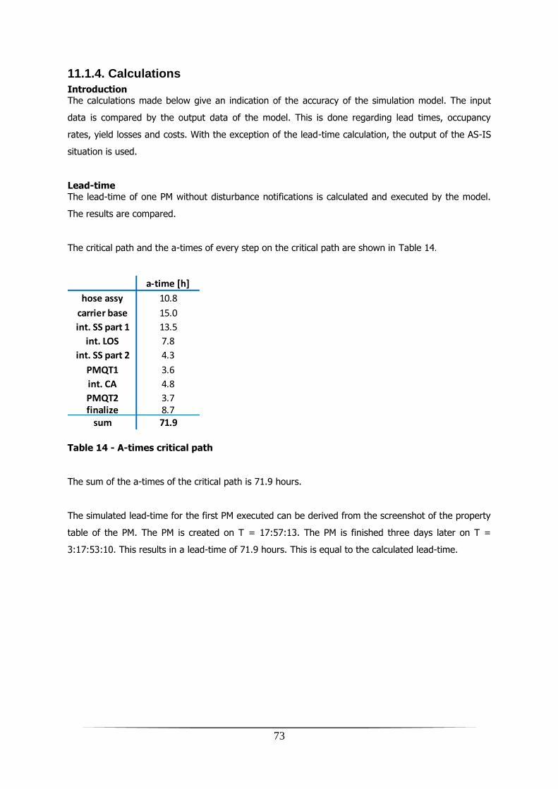
73

11.1.4. Calculations

Introduction The calculations made below give an indication of the accuracy of the simulation model. The input

data is compared by the output data of the model. This is done regarding lead times, occupancy

rates, yield losses and costs. With the exception of the lead-time calculation, the output of the AS-IS

situation is used.

Lead-time The lead-time of one PM without disturbance notifications is calculated and executed by the model.

The results are compared.

The critical path and the a-times of every step on the critical path are shown in Table 14.

Table 14 - A-times critical path

The sum of the a-times of the critical path is 71.9 hours.

The simulated lead-time for the first PM executed can be derived from the screenshot of the property

table of the PM. The PM is created on T = 17:57:13. The PM is finished three days later on T =

3:17:53:10. This results in a lead-time of 71.9 hours. This is equal to the calculated lead-time.

a-time [h]

hose assy 10.8

carrier base 15.0

int. SS part 1 13.5

int. LOS 7.8

int. SS part 2 4.3

PMQT1 3.6

int. CA 4.8

PMQT2 3.7finalize 8.7

sum 71.9

74

Figure 41 - Creation time and finish time of a PM

Occupancy rate of INT_SS workstation

The occupancy rate of the bottleneck of the process, the „int. SS‟ workstation, is now calculated and

compared with the simulation result.

Table 15 - Simulated processing time of 'int SS' workstation

The workcontent for the INT_SS workstation is simulated to be 272.43 hours/week, assuming an

output rate of 11 PM‟s/week. The measured workcontent of the INT_SS workstation is the

workcontent of the „INT SS part 1‟ process plus the „INT SS part 2‟ process, multiplied by the output

rate of 11 PM/ week. The workcontent is calculated by the the a-time of a process plus the b-chance

times the MTTR. Data is given in the tables of appendix J.

workcontent „int. SS‟ 1 = 18.49 hour

int SS

average occupancy rate 81.1%

stations 4.00

hours/week 84.00

total processing time [hours] 272.43

75

workcontent „int. SS‟ 2 = 6.10 hour

The total workcontent is equal to 18.49 + 6.10 = 24.59 hour. Multiplying this workcontent by the

output rate:

𝑡𝑜𝑡𝑎𝑙 𝑝𝑟𝑜𝑐𝑒𝑠𝑠𝑖𝑛𝑔 𝑡𝑖𝑚𝑒 = 24.59 ∗ 11 = 270.52 𝑕𝑜𝑢𝑟𝑠

This results in a difference of 0.7% with the simulation results.

Yield

The yield loss is measured from the simulation and calculated. The results are compared.

The repair chance per PM type is given in the table below. With the product mix, the consolidated

yield loss can be calculated. This is stated to be 32.2%.

Table 16 - Yield breakdown

The data of appendix L is used as input for the simulation model. The output is compiled as follows:

Output repair = 2.38 PM/week

Output quick fix = 1.21 PM/week

Output build = 7.39 PM/week

Output total = 10.97 PM/week

𝑆𝑖𝑚𝑢𝑙𝑎𝑡𝑒𝑑 𝑦𝑖𝑒𝑙𝑑 % =10.97 − 3.59

10.97= 67.4%

𝐶𝑎𝑙𝑐𝑢𝑙𝑎𝑡𝑒𝑑 𝑦𝑖𝑒𝑙𝑑[%] = 1 − 0.322 = 67.7%

𝐷𝑖𝑓𝑓𝑒𝑟𝑒𝑛𝑐𝑒 = 67.7 − 67.4 = 0.3%

Costs

productmix repairchanceproductmix *

repairchance

PM311LEX 16.7% 33% 0.055

PM311REX 16.7% 28% 0.047

PM321LEX 33.3% 32% 0.107

PM321REX 33.3% 34% 0.113

sum 0.322

76

The experiment has been run with 12 subassy operators and 11 integration operators, in total 23

operators. These operators are 84 hours/week available. The cost price of one operator is 46

euro/hour.

𝑙𝑎𝑏𝑜𝑟𝑐𝑜𝑠𝑡𝑠/𝑦𝑒𝑎𝑟 = 23 ∗ 46 ∗ 84 ∗ 52 = 4621344 𝑒𝑢𝑟𝑜

This is equal to the simulated labor costs. Occupancy rate of the operators is not taken into account

for the determination of the labor costs, since costs are a result of the effective available presence

time.

Calculation of the capital costs of the WIP is based on the lead-time and the buffer time.

The average buffersize of the experiment is 9.55 PM‟s. With a moverate of 11 PM/week the average

buffer time per PM can be calculated:

𝑏𝑢𝑓𝑓𝑒𝑟𝑡𝑖𝑚𝑒 = 9.55 ∗ 7.39/10.97 = 6.44 𝑑𝑎𝑦𝑠

The simulated average lead-times and buffer times are shown in the table below:

Table 17 - Simulated lead times and buffer times

The average delivery time per build PM is calculated:

𝑑𝑒𝑙𝑖𝑣𝑒𝑟𝑦𝑡𝑖𝑚𝑒 = 14.85 + 6.44 + 11.90 + 6.44 ∗2.37

7.39+ 6.87 ∗

1.21

7.39= 28.3 𝑑𝑎𝑦𝑠

The capital costs per year follows from the delivery time, the output of build PMs (7.39 PM/week), the

WACC (=8%) and the costs of goods of a PM (825000 euro):

𝑐𝑎𝑝𝑖𝑡𝑎𝑙𝑐𝑜𝑠𝑡𝑠/𝑦𝑒𝑎𝑟 = 28.3 ∗ 7.39 ∗ 52 ∗ 825000 ∗0.08

365= 1966461 𝑒𝑢𝑟𝑜

The capital costs of the simulation experiment are 1995950 euro. This is a difference of 29489 euro

or 1.5%.

regular repair quick fix repair

leadtime [days] 14.85 11.90 6.87

buffertime [days] 6.44 6.44 0.00

77

The scrap costs per rejected PM are shown in appendix D. The following calculation gives the yearly

scrap costs:

𝑠𝑐𝑟𝑎𝑝𝑐𝑜𝑠𝑡𝑠/𝑦𝑒𝑎𝑟 = 4139 ∗ (2.38 + 1.21) ∗ 52 = 770901 𝑒𝑢𝑟𝑜

This equals the costs given by the simulation model.

11.1.5. Conclusion

The simulation model is verified by visualization, tracing and calculations. Deviations up to 1.5% are

noticed. This shows that the model, regarding of the small deviations, works as intended.

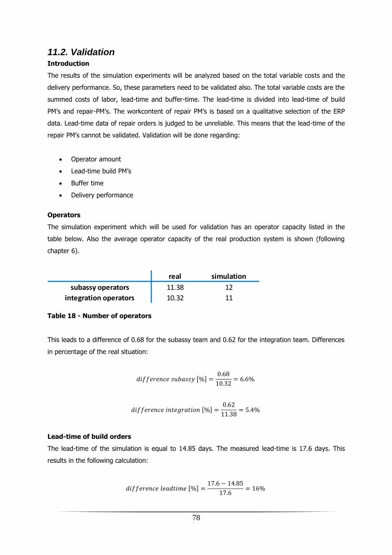
78

11.2. Validation Introduction

The results of the simulation experiments will be analyzed based on the total variable costs and the

delivery performance. So, these parameters need to be validated also. The total variable costs are the

summed costs of labor, lead-time and buffer-time. The lead-time is divided into lead-time of build

PM‟s and repair-PM‟s. The workcontent of repair PM‟s is based on a qualitative selection of the ERP

data. Lead-time data of repair orders is judged to be unreliable. This means that the lead-time of the

repair PM‟s cannot be validated. Validation will be done regarding:

Operator amount

Lead-time build PM‟s

Buffer time

Delivery performance

Operators

The simulation experiment which will be used for validation has an operator capacity listed in the

table below. Also the average operator capacity of the real production system is shown (following

chapter 6).

Table 18 - Number of operators

This leads to a difference of 0.68 for the subassy team and 0.62 for the integration team. Differences

in percentage of the real situation:

𝑑𝑖𝑓𝑓𝑒𝑟𝑒𝑛𝑐𝑒 𝑠𝑢𝑏𝑎𝑠𝑠𝑦 % =0.68

10.32= 6.6%

𝑑𝑖𝑓𝑓𝑒𝑟𝑒𝑛𝑐𝑒 𝑖𝑛𝑡𝑒𝑔𝑟𝑎𝑡𝑖𝑜𝑛 % =0.62

11.38= 5.4%

Lead-time of build orders

The lead-time of the simulation is equal to 14.85 days. The measured lead-time is 17.6 days. This

results in the following calculation:

𝑑𝑖𝑓𝑓𝑒𝑟𝑒𝑛𝑐𝑒 𝑙𝑒𝑎𝑑𝑡𝑖𝑚𝑒 % =17.6 − 14.85

17.6= 16%

real simulation

subassy operators 11.38 12

integration operators 10.32 11

79

There must be remarked that a slightly lower operator capacity from 11 integration operators to an

average of 10.32 integration operators will lead to a longer lead time. As a matter of fact, the

difference will then be lower than 16%.

Buffersize

The average buffersize as a result of the simulation is 9.5 PM‟s. The measured average buffersize is

9.9 PM‟s. This leads to the following calculation to determine the difference.

𝑑𝑖𝑓𝑓𝑒𝑟𝑒𝑛𝑐𝑒 𝑏𝑢𝑓𝑓𝑒𝑟𝑠𝑖𝑧𝑒 % =9.9 − 9.5

9.9= 4%


The delivery performance of the simulation is 81%. The measured delivery performance is 82%. This

leads to a difference of 1%.

Conclusion

The simulation model is validated with deviations noticed up to 16%.

80

81

12. Confidence analysis

12.1. Introduction A confidence analysis is executed to be able to quantify the quality of the experiments as a result of

the amount of observations per experiment. As one knows, a high amount of observations leads to a

better predictable mean of an output parameter. Coincide of a high amount of observations is the

required simulation time. Since there are a huge amount of experiments planned to be executed, the

amount of observations has to be limited. The amount of observations is chosen to be 20. In this

analysis the confidence of the output parameters with this amount of observations is evaluated.

The 95% confidence interval of the variable costs and the delivery performance will be calculated.

The amount of samples is lower than 30, so according to [Richard I. Levin, 1978] the t-distribution is

required. The t-value for a 95% confidence interval and a sample size of 20 is 2.093. The 95%

confidence interval is calculated as follows:

𝐸𝑞. 12.1 0.95 = 𝑃 𝑋 − 𝑡 ∗𝜎

𝑛< 𝜇 < 𝑋 + 𝑡 ∗

𝜎

𝑛

Where t is the student‟s t-distribution value, 𝑋 is the sample mean, n is the sample size and σ is the

sample standard deviation.

The output parameters to be evaluated are

Total variable costs per PM (labor + capital costs WIP)


The output data of the simulated AS-IS situation will be used.

12.2. Total variable costs The sample mean is 17576 euro and the sample standard deviation is 600 euro. The lower and upper

boundaries of the interval are calculated:

𝐸𝑞. 12.2 𝑙𝑜𝑤𝑒𝑟 𝑖𝑛𝑡𝑒𝑟𝑣𝑎𝑙 𝑏𝑜𝑢𝑛𝑑 = 𝑋 − 𝑡 ∗𝜎

𝑛= 18883 − 2.093 ∗

311

20= 18737 𝑒𝑢𝑟𝑜

𝐸𝑞. 12.3 𝑢𝑝𝑝𝑒𝑟 𝑖𝑛𝑡𝑒𝑟𝑣𝑎𝑙 𝑏𝑜𝑢𝑛𝑑 = 𝑋 + 𝑡 ∗𝜎

𝑛= 18883 + 2.093 ∗

311

20= 19029 𝑒𝑢𝑟𝑜

Subtracting the upper and lower interval bound gives an interval size of 292 euro. This results in a

deviation of:

82

𝑑𝑒𝑣𝑖𝑎𝑡𝑖𝑜𝑛 =292/2

18883= 0.77%

With 95% certainty it can be concluded that the mean will be in the range of 18883 ± 0.77%.

12.3. Delivery performance The sample mean is 0.814 percent and the sample standard deviation is 0.079. The lower and upper

boundaries of the interval are calculated:

𝐸𝑞. 12.4 𝑙𝑜𝑤𝑒𝑟 𝑖𝑛𝑡𝑒𝑟𝑣𝑎𝑙 𝑏𝑜𝑢𝑛𝑑 = 𝑋 − 𝑡 ∗𝜎

𝑛= 0.814 − 2.093 ∗

0.077

20= 0.775 𝑝𝑒𝑟𝑐𝑒𝑛𝑡

𝐸𝑞. 12.5 𝑢𝑝𝑝𝑒𝑟 𝑖𝑛𝑡𝑒𝑟𝑣𝑎𝑙 𝑏𝑜𝑢𝑛𝑑 = 𝑋 + 𝑡 ∗𝜎

𝑛= 0.814 + 2.093 ∗

0.077

20= 0.853 𝑝𝑒𝑟𝑐𝑒𝑛𝑡

Subtracting the upper and lower interval bound gives an interval size of 0.072 percent. This results in

a deviation of:

𝑑𝑒𝑣𝑖𝑎𝑡𝑖𝑜𝑛 =0.077/2

0.814= 4.84%

With 95% certainty it can be concluded that the mean will be in the range of 0.814 ± 4.84%.

The confidence intervals of the total variable costs and the delivery performance of all experiments

are shown in appendix M.

12.4. Conclusion The confidence intervals of all experiments are smaller than the determined deviations from the

validation of the simulation model. Therefore it is concluded that a number of observations of 20 per

experiment is sufficient.

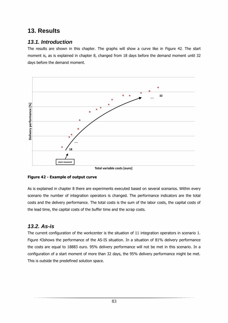
83

13. Results

13.1. Introduction The results are shown in this chapter. The graphs will show a curve like in Figure 42. The start

moment is, as is explained in chapter 8, changed from 18 days before the demand moment until 32

days before the demand moment.

Figure 42 - Example of output curve

As is explained in chapter 8 there are experiments executed based on several scenarios. Within every

scenario the number of integration operators is changed. The performance indicators are the total

costs and the delivery performance. The total costs is the sum of the labor costs, the capital costs of

the lead time, the capital costs of the buffer time and the scrap costs.

13.2. As-is The current configuration of the workcenter is the situation of 11 integration operators in scenario 1.

Figure 43shows the performance of the AS-IS situation. In a situation of 81% delivery performance

the costs are equal to 18883 euro. 95% delivery performance will not be met in this scenario. In a

configuration of a start moment of more than 32 days, the 95% delivery performance might be met.

This is outside the predefined solution space.

De

live

ry p

erf

orm

ance

[%

]

Total variable costs [euro]

DP vs Costs

18

32

....

....

start moment

84

Figure 43 - AS-IS configuration

Table 19 - AS-IS configuration

The delivery performance-costs curve is a result of the change of the start moment only. At low start

moments, the buffersize is low. This results in a low delivery performance. Due to the low buffersize

PM‟s have a low buffer time. Therefore the capital costs of the buffer time (as part of the total costs)

are low also. Opposite, at high start moment values, the buffersize increases. Therefore the delivery

performance increases and the capital costs of the buffer time increases. Every increase of delivery

performance requires a higher increase of the buffersize (and therefore higher increase of costs). This

results in the curved plot.

0.4

0.5

0.6

0.7

0.8

0.9

1

17000 17500 18000 18500 19000 19500 20000 20500 21000

De

live

ry p

erf

orm

ance

[%

]


Scenario 1, 11 int. operators

Experiment 50

start moment 26 days

integration operators 11

delivery performance 82%

total costs 18883 euro

Scenario 1: AS-IS

85

13.3. Increasing delivery performance

13.3.1. Results

Scenario 1

All output values of the simulation experiments of scenario 1 are shown in Figure 44.As can be seen,

an optimal number of operators can be derived from the plot. The output results show that the

configuration of 10 integration operators performs worse than the configuration of 11 integration

operators. Both the configuration of 11 operators and the configuration of 12 operators do show the

lowest costs with equal delivery performance. Delivery performances lower than 77% leads to lower

costs in the 11 operator configuration than in the 12 operator configuration. Higher delivery

performance leads to the opposite. The configurations of 13, 14 and 15 operators do perform worse

again than the configurations of 11 or 12 operators, although on the highest delivery performance

levels, the configuration of 13 operators equals the configuration of 12 operators.

Figure 44 - Scenario 1

The 11, 12 and 13 operator configurations do have almost equal performance curves. The 10, 14 and

15 operator configurations explicitly underperform. This is explicable as follows. A low number of

operators lead to high occupancy rates. This results in high lead-times. Due to high lead-times,

delivery performance decreases. Opposite, a high number of operators results in low lead-times and

thus a high delivery performance. But there is more available labor, which results in increasing labor-

costs.

40%

50%

60%

70%

80%

90%

100%

17000 18000 19000 20000 21000 22000 23000

De

live

ry p

erf

orm

ance

[%

]


Scenario 1

10 int. operators

11 int. operators

12 int. operators

13 int. operators

14 int. operators

15 int. operators

86

When zooming in on the delivery performances higher than 95%, one sees that the configuration of

13 operators does have the lowest costs, although there is hardly a difference with the configuration

of 12 and 14 operators. This leads to a value of 20152 euro per PM.

Figure 45 - Scenario 1: DP > 95%

The experiment of scenario 1 which meets the requirements does have the properties shown in Table

20.

Table 20 - Best performing configuration of Scenario 1

Scenario 2

Scenario 2 is executed with the workstation configuration as in the current situation plus one

workstation for the bottleneck („int SS‟ workstation). The current number of integration operators, 11

operators, does not result in the best performance. At lower delivery performance levels, the

configuration of 12 operators results in the lowest total costs. At higher delivery performances, the

configuration of 13 operators results in the lowest total costs. This phenomenon is already explained

in the text of scenario 1.

95.0%

95.5%

96.0%

96.5%

97.0%

97.5%

98.0%

98.5%

99.0%

99.5%

100.0%

19000 19500 20000 20500 21000 21500 22000 22500

De

live

ry p

erf

orm

ance

[%

]


Scenario 1: DP > 95%

10 int. operators

11 int. operators

12 int. operators

13 int. operators

14 int. operators

15 int. operators

Experiment 64





Scenario 1

87



40%

50%

60%

70%

80%

90%

100%

17000 18000 19000 20000 21000 22000 23000

De

live

ry p

erf

orm

ance

[%

]


Scenario 2

10 int. operators

11 int. operators

12 int. operators

13 int. operators

14 int. operators

15 int. operators

95.0%

95.5%

96.0%

96.5%

97.0%

97.5%

98.0%

98.5%

99.0%

99.5%

100.0%

19000 19500 20000 20500 21000 21500 22000 22500

De

live

ry p

erf

orm

ance

[%

]



10 int. operators

11 int. operators

12 int. operators

13 int. operators

14 int. operators

15 int. operators

88

When zooming in onto the 95% delivery performance level in Figure 47, one sees that the

configuration of 13 integration operators results in total costs of 19475 euro. The properties of this

experiment are shown in Table 21. The benefits of the extra workstation are only noticeable in the

high operator configurations, since these do have a substantial higher delivery performance in

scenario 2 than in scenario 1. The reason for this noticeable difference at high operator numbers is

that there is a bottleneck transition from the operator team to the „int SS‟ workstationgroup. There

has to be remarked that the differences of about two percent-points have still to be considered very

small.

Table 21 - Best performing configuration of scenario 2

Scenario 3

Scenario 3 is a scenario with three repair-stations. This scenario has the same workstation resources

as scenario 1. For that reason, one „chuck assy‟ station, one „int SS‟ station and one „int CA‟ station

are removed, as is stated before. The change in workstation occupancy rates is shown in the figures

of appendix K.

The configuration of 12 and 13 operators results in the lowest costs. Again this phenomenon is

already explained in the text of scenario 1, although for low operator numbers, scenario three is more

extreme with occupancy rate up to 100%. This results in a loss of output and therefore the moverate

requirement is not met for the 10 operator scenario. It has to be concluded that for low operator/high

occupancy rate configurations scenario three underperforms in comparison to scenario 1. This is

caused by increasing inflexibility when allocating the operator resources to the PM‟s.

When zooming in into the 95% delivery performance level, the lowest costs are needed for the

configuration of 12 operators. The costs of this configuration are 19714 euro. The properties of this

experiment are shown in table 22.

Experiment 46





Scenario 2

89



40%

50%

60%

70%

80%

90%

100%

17000 18000 19000 20000 21000 22000 23000

De

live

ry p

erf

orm

ance

[%

]


Scenario 3

7 int (+3 rep.) operators

8 int.(+3 rep.) operators





95.0%

95.5%

96.0%

96.5%

97.0%

97.5%

98.0%

98.5%

99.0%

99.5%

100.0%

19000 19500 20000 20500 21000 21500 22000 22500

De

live

ry p

erf

orm

ance

[%

]



7 int (+3 rep.) operators






90


Scenario 4

Scenario 4 is equal to scenario 3, with one difference. One extra repair-station is added. This results

in four repair-stations in total. This scenario equals scenario 2 when considering workstation

resources. Also the integration operators are altered again. The sum of the integration and the repair

operators results in equal operator capacities as in the other three scenarios.


The configuration with the best performance regarding costs and delivery performance is the

configuration of 12 and 13 operators (respectively green and purple in Figure 50). The zoom-in into

the 95% delivery performance level gives Figure 51. It becomes clear that the configuration with the

lowest costs is the configuration of 12 operators. This configuration results in total costs of 19697

euro.

Experiment 63


integration operators 9(+3)



Scenario 3

40%

50%

60%

70%

80%

90%

100%

17000 18000 19000 20000 21000 22000 23000

De

live

ry p

erf

orm

ance

[%

]


Scenario 4

6 int.(+ 4 rep.) operators






91


The properties of the best performing configuration are shown in Table 23.


13.3.2. Comparing the scenarios Out of all four scenarios the best performing scenario is selected. From the analysis of the output

graphs it becomes clear that scenario 2 result in the lowest costs with a delivery performance of more

than 95%. These costs are 19475 euro. The properties of the best performing configuration of this

scenario are shown again in Table 24.

95.0%

95.5%

96.0%

96.5%

97.0%

97.5%

98.0%

98.5%

99.0%

99.5%

100.0%

19000 19500 20000 20500 21000 21500 22000 22500

De

live

ry p

erf

orm

ance

[%

]



6 int.(+ 4 rep.) operators






Experiment 63


integration operators 8(+4)



Scenario 4

92

Table 24 - Best performing configuration of all scenarios

It must be remarked that the best performing configurations of all four scenarios have a relative small

difference regarding costs. Table 25 gives a view of the total costs of every scenario and the 95%

confidence interval from the confidence analysis. The difference between scenario 2 and the next

best scenario (scenario 4) is large enough to ensure there is a statistical significant difference,

although it is a very small difference.

Table 25 - Two-sided confidence intervals of the best performing configurations

13.3.3. Robustness

By comparing the scenarios it is concluded that the best performing configuration is reached by:

1. Increasing the number of integration operators by 2 to 13 operators.

2. Increasing the number of „integrate SS‟ workstations by 1 to 5.

To investigate robustness of this conclusion, results of the confidence analysis are used. There‟s

searched for configurations which do perform lower than 95% delivery performance, but are close to

the best performing configuration. From these configurations the confidence intervals are shown in

Figure 52and Figure 53.

From Figure 52it is concluded that no there is no statistical significant difference between the four

scenarios near the 95% delivery performance level. Therefore no robust recommendation can be

done regarding the production structure and the number of workstations.

Experiment 46





Scenario 2

total costs [euro]

two-sided

confidence

interval [euro]

Scenario 1 20152 223




93

Figure 52 - Confidence intervals of configurations of multiple scenarios

From Figure 53it is concluded that no there is no statistical significant difference between the two

operator configurations of scenario 1 near the 95% delivery performance level. Therefore no robust

recommendation can be done regarding the number of workstations.

Figure 53 - Confidence intervals of multiple configurations of the same scenario

One could conclude that the number of observations (20 runs per experiment) is not sufficient. Since

the confidence intervals as percentage of the result values (for every experiment) are way smaller

than the difference percentages found during validation of the model (as shown in appendix M), the

recommendations won‟t be more robust by increasing the number of observations.

The recommendation of improving the workcenter with one extra „int. SS‟ workstation and two extra

integration operators is a non-robust recommendation. As becomes clear from the plotted figures

there are small differences noticeable between the scenarios in suboptimal regions of the delivery

0.93

0.94

0.95

0.96

0.97

0.98

0.99

1

19000 19200 19400 19600 19800 20000

De

live

ry p

erf

orm

ance

[%

]


Confidence analysis

Scenario 2, 13 operators, start 25(best performing)Scenario 1, 12 operators, start 27

Scenario 3, 12 operators, start 27


0.93

0.94

0.95

0.96

0.97

0.98

0.99

1

19000 19500 20000 20500 21000

De

live

ry p

erf

orm

ance

[%

]


Confidence analysis

scenario 1, 13 operators, start 28(best performing)

scenario 1, 12 operators, start 29

94

performance-costs plots, but all four scenarios are able to reach such a performance in the optimal

regions that there cannot be made a robust distinction between these scenarios. Therefore there has

to be searched for an alternative in order to be able to recommend on the optimal number of

operators and the optimal startmoment.

13.3.4. Rule-of-thumb occupancy rate

An alternative recommendation can be found in the occupancy rate of the operators. In Table 26 the

occupancy rates of the integration operator teams are shown of the best performing configurations of

all four scenarios. In the utmost right column also the occupancy rates of the second best

configuration is shown. These second best configurations are selected based on the delivery

performance-cost curves of all four scenarios. As one can see in the curve graphs, the best operator

configuration and the second best configuration are very close to each other at the 95% delivery

performance level.

Table 26 - Occupancy rates of the best performing configurations of all scenarios

It can be concluded that the production system has to be equipped with operator teams which meet

an occupancy rate of 78±5%. The occupancy rates can be divided into two ranges, a ‟73-74%‟ range

and a ‟80-82%‟ range. This is clear since two numbers of operators are shown, the configuration of

12 operators and the configuration of 13 operators.

Table 27 - Occupancy rates as a result of a sensitivity analysis

A sensitivity analysis is performed to determine whether this rule-of-thumb also fits with different

workcontent amounts. Experiments with scenario 1 are executed with decreased b-time and

DPOR of best

configuration

OR of second best

configuration

Scenario 1 AS-IS (11 int. oper.) 82% 87%

Scenario 1: 13 -- 12 oper. 95% 73% 79%

Scenario 2: 13 -- 12 oper. 95% 74% 80%

Scenario 3: 12 -- 13 oper. 95% 82% 74%

Scenario 4: 12 -- 13 oper. 95% 81% 74%

average 78% 77%

Occupancy rates

DP

occupancy

rates of best

configuration

Scenario 1, - 10% btime 95% 83%

Scenario 1, -30% btime 95% 76%

Scenario 1, yield 88% 95% 76%

Scenario 1, yield 100% 95% 76%

average 78%

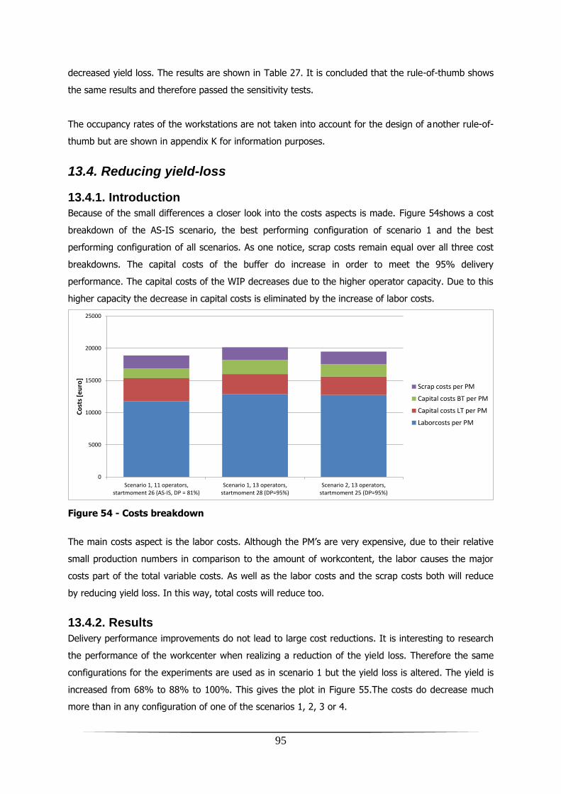
95

decreased yield loss. The results are shown in Table 27. It is concluded that the rule-of-thumb shows

the same results and therefore passed the sensitivity tests.

The occupancy rates of the workstations are not taken into account for the design of another rule-of-

thumb but are shown in appendix K for information purposes.

13.4. Reducing yield-loss

13.4.1. Introduction

Because of the small differences a closer look into the costs aspects is made. Figure 54shows a cost

breakdown of the AS-IS scenario, the best performing configuration of scenario 1 and the best

performing configuration of all scenarios. As one notice, scrap costs remain equal over all three cost

breakdowns. The capital costs of the buffer do increase in order to meet the 95% delivery

performance. The capital costs of the WIP decreases due to the higher operator capacity. Due to this

higher capacity the decrease in capital costs is eliminated by the increase of labor costs.

Figure 54 - Costs breakdown

The main costs aspect is the labor costs. Although the PM‟s are very expensive, due to their relative

small production numbers in comparison to the amount of workcontent, the labor causes the major

costs part of the total variable costs. As well as the labor costs and the scrap costs both will reduce

by reducing yield loss. In this way, total costs will reduce too.

13.4.2. Results

Delivery performance improvements do not lead to large cost reductions. It is interesting to research

the performance of the workcenter when realizing a reduction of the yield loss. Therefore the same

configurations for the experiments are used as in scenario 1 but the yield loss is altered. The yield is

increased from 68% to 88% to 100%. This gives the plot in Figure 55.The costs do decrease much

more than in any configuration of one of the scenarios 1, 2, 3 or 4.

0

5000

10000

15000

20000

25000

Scenario 1, 11 operators,startmoment 26 (AS-IS, DP = 81%)

Scenario 1, 13 operators,startmoment 28 (DP=95%)

Scenario 2, 13 operators,startmoment 25 (DP=95%)

Co

sts

[eu

ro]

Scrap costs per PM

Capital costs BT per PM

Capital costs LT per PM

Laborcosts per PM

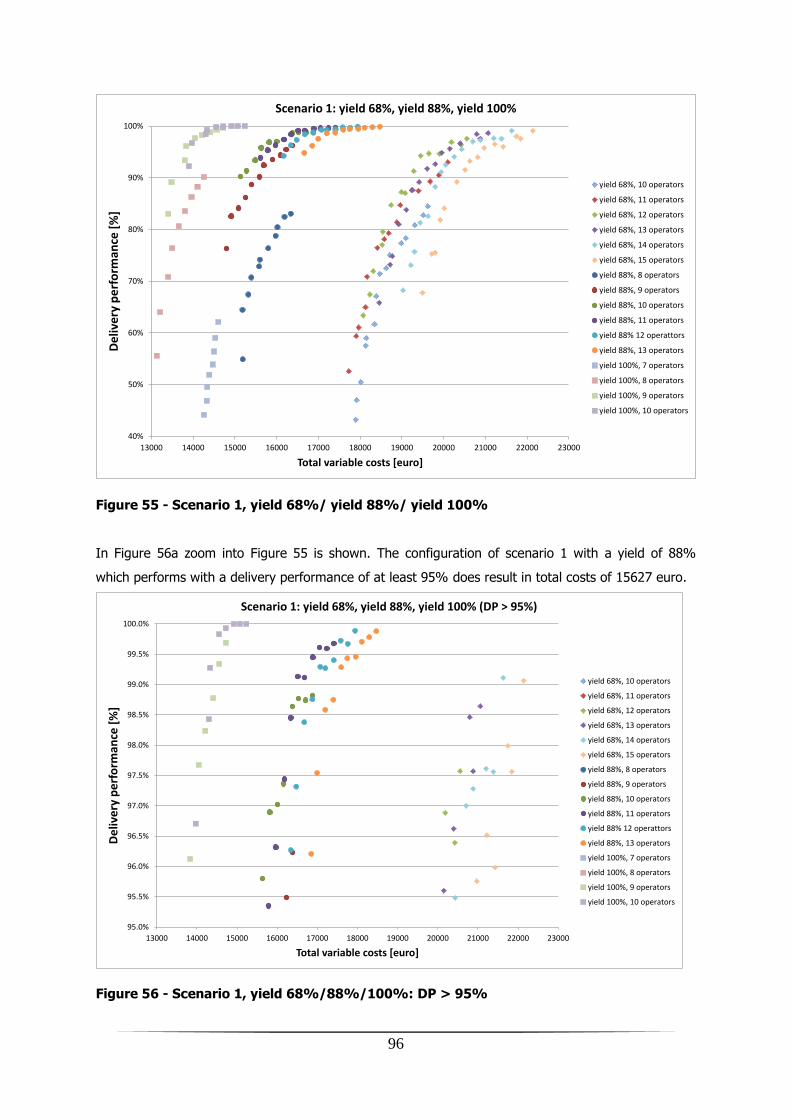
96

Figure 55 - Scenario 1, yield 68%/ yield 88%/ yield 100%

In Figure 56a zoom into Figure 55 is shown. The configuration of scenario 1 with a yield of 88%

which performs with a delivery performance of at least 95% does result in total costs of 15627 euro.

Figure 56 - Scenario 1, yield 68%/88%/100%: DP > 95%

40%

50%

60%

70%

80%

90%

100%

13000 14000 15000 16000 17000 18000 19000 20000 21000 22000 23000

De

live

ry p

erf

orm

ance

[%

]


Scenario 1: yield 68%, yield 88%, yield 100%

yield 68%, 10 operators










yield 88% 12 operattors






95.0%

95.5%

96.0%

96.5%

97.0%

97.5%

98.0%

98.5%

99.0%

99.5%

100.0%

13000 14000 15000 16000 17000 18000 19000 20000 21000 22000 23000

De

live

ry p

erf

orm

ance

[%

]


Scenario 1: yield 68%, yield 88%, yield 100% (DP > 95%)

















97

The costs breakdowns of the three yield levels are shown in Figure 57. The costs of the best

performing configuration of the „yield 88%‟ scenario decreases largely in comparison to the best

performing configuration of scenario 1, as is expected. Costs are further decreased when increasing

yield to 100%.

Figure 57 - Cost breakdown of scenario 1, yield 68%/ 88%/ 100%

It can be concluded that, although workcontent only increased with about 25% due to the yield loss

of 32% (as stipulated in chapter 6), the total variable costs increases with a percentage of about

(20152-13831)/13831 =45%. Thus, yield loss does not only lead to increasing labor, but also

substantially negative influence the capital costs and scrap costs.

The economic value of a yield improvement to 88% can now easily be calculated. Assuming a delivery

performance increase within the current scenario to 95%, total variable costs per PM are 20152 euro.

With a moverate of regular PMs of 7.4 PM‟s/week and a cost reduction of 20152-15627=4525 euro

the cost reduction on a yearly basis is:

𝑦𝑒𝑎𝑟𝑙𝑦 𝑐𝑜𝑠𝑡 𝑟𝑒𝑑𝑢𝑐𝑡𝑖𝑜𝑛 = 4525 ∗ 7.4 ∗ 52 = 1741𝑘 𝑒𝑢𝑟𝑜

Assuming the moverate to be reduced to 4 PM‟s/week for example as a result of an economic

downturn the costs will be lower:

𝑦𝑒𝑎𝑟𝑙𝑦 𝑐𝑜𝑠𝑡 𝑟𝑒𝑑𝑢𝑐𝑡𝑖𝑜𝑛 = 4525 ∗ 4 ∗ 52 = 941𝑘 𝑒𝑢𝑟𝑜

0

5000

10000

15000

20000

25000

Scenario 1, 13 operators, startmoment 28(DP=95%)

Scenario 1 Yield 88%, 10 operators,startmoment 21 (DP=95%)


Co

sts

[eu

ro]

Scrap costs per PM



Laborcosts per PM

98

13.4.3. Rule-of-thumb startmoment

In every executed scenario the performance of the production system is optimal with an occupancy

rate of integration operators of 78±5%. This rule-of-thumb gives information about the resources of

the production system and has the result that the lowest delivery performance-costs curve will be

reached. But to reach a delivery performance of 95%, another rule is required, which gives

information about the production control. A rule-of-thumb can be defined for the relation between

start moment and yield loss. The startmoments of the three yield loss scenarios are plotted in Figure

58. The startmoment needs to be increased linearly (from a constant value of 17 days in the case of

100% yield) with the yield loss in order to reach a delivery performance of 95%.

Figure 58 - Start moments at different yield losses

After determination of the optimal amount of resources, the start moment is related to the yield loss

as follows:

Eq. 13.1 𝑠𝑡𝑎𝑟𝑡𝑚𝑜𝑚𝑒𝑛𝑡 = a ∗ 𝑦𝑖𝑒𝑙𝑑𝑙𝑜𝑠𝑠 + 𝑏 ∗𝑤𝑜𝑟𝑘𝑐𝑜𝑛𝑡𝑒𝑛𝑡

𝑤𝑜𝑟𝑘𝑐𝑜𝑛𝑡𝑒𝑛𝑡 𝐴𝑆 −𝐼𝑆

startmoment [days] : The number of days before the demand moment to start the production.

a : Constant of value 34

b :Constant of value 17 (note: without yield-loss the startmoment is 17 days)

yield-loss [%] : The yield-loss expressed in percentage.

workcontent [h] : The workcontent expressed in hours.

workcontentAS-IS : The workcontent of the current situation is 202 hours.

Boundary conditions for scaling the startmoment by means of the workcontent:

10

15

20

25

30

35

0% 4% 8% 12% 16% 20% 24% 28% 32% 36%

Star

t m

om

en

t [d

ays]

Yield loss [%]

yield-level scenarios

y=34x+17

99

• The ratio of workcontent between regular and repair operations must remain unchanged.

Even so, the distribution of a-time and b-time must remain unchanged.

• Occupancy rates of resources must remain unchanged.

13.4.4. Conclusion

Increasing the delivery performance has to be performed by adjusting the capacity of the current

operator resources by 2 operators to 13 operators. The endbuffer has to be filled with an average

number of 13 PM‟s. This has to be realized by starting the regular build PM‟s 28 days before the

demand date. This implies that the buffer is composed in proportions equal to the production-mix.

After applying data of the confidence analysis there has to be concluded that no robust

recommendation can be done regarding the number of operators, the scenario type and the

startmoment.

A breakdown of costs shows that labor takes the largest part of the total costs. A significant reduction

in labor and scrap can only be reached by reducing the yield loss.

Two rules-of-thumb are defined.

1. Operator capacity needs to be adjusted to a level of 78±5% occupancy rate.

2. The start moment is related to the yield loss by the relation:


𝑤𝑜𝑟𝑘𝑐𝑜𝑛𝑡𝑒𝑛𝑡𝐴𝑆−𝐼𝑆


• The ratio of workcontent between regular and repair operations must remain unchanged.

Even so, the distribution of a-time and b-time must remain unchanged.


The economic value of a yield improvement from 68% to 88% results in a yearly financial benefit of

1741k euro when an average moverate of 7.4 regular build PM‟s per week takes place. A yearly

financial benefit of 941k euro takes place with an average moverate of 4 regular build PM‟s per week.

100

101

14. Conclusions The goal of this research is to determine a configuration of the workcenter which meets:




This is reached by solving problems as described in the problem statement of chapter 7.

The reject trajectory has to be improved by adding several control loops. A description is given of the

required information for the control loops. The study to this trajectory has led to execution of the

control by a real-time dashboard.

The simulation model is explained by process description language. It is verified and validated and an

extensive confidence analysis has been performed. These analyses shows that the model works as

intended and that confidence intervals are small enough to use the output data for further analysis.

Simulation is used to investigate several scenarios. Conclusions of the simulation results are stipulated

below.

Increasing the delivery performance has to be performed by adjusting the capacity of the current

operator resources by 2 operators to 13 operators. The endbuffer has to be filled with an average

number of 13 PM‟s. This has to be realized by starting the regular build PM‟s 28 days before the

demand date. This implies that the buffer is filled in the proportions equal to the production-mix.

After applying data of the confidence analysis there has to be concluded that no robust

recommendation can be done regarding the number of operators, the scenario type and the

startmoment.

A breakdown of costs shows that labor takes thelargest part of the total costs. A significant reduction

in labor and scrap can only be reached by reducing the yield loss.

In every executed scenario the performance of the production system is optimal with an occupancy

rate of integration operators of 78±5%. As a rule-of-thumb this percentage can be used to determine

optimal operator resources. After determination of the amount of resources, the start moment is

related to the yield loss as follows:


𝑤𝑜𝑟𝑘𝑐𝑜𝑛𝑡𝑒𝑛𝑡𝐴𝑆−𝐼𝑆

102

Where the variables and constants are stated as follows:

startmoment [days] : The number of days before the demand moment to start the production.

a : Constant of value 34

b : Constant of value 17 (note: without yield-loss the startmoment is 17 days)

yield-loss [%] : The yield-loss expressed in percentage.

workcontent [h] : The workcontent expressed in hours.

workcontentAS-IS : The workcontent of the current situation is 202 hours.


• The ratio of workcontent per PM between regular and repair operations must remain

unchanged. Even so, the distribution of a-time and b-time must remain unchanged.


The economic value of a yield improvement from 68% to 88% results in a yearly financial benefit of

1741k euro when an average moverate of 7.4 regular build PM‟s per week takes place. A yearly

financial benefit of 941k euro takes place with an average moverate of 4 regular build PM‟s per week.

103

15. Recommendations In this research it is assumed that a fixed start moment in relation to the demand moment takes

place. The start moment is quantified in different scenarios, but no research is done to temporary

adjustments of the start moment. Further research to the use of adapted production control might

lead to an improved production system.

The required delivery performance of 95% is arbitrarily determined, since it is extremely difficult to

determine costs of a PM being delivered too late. These costs are not only a function of operating

costs/WIP costs of the different succeeding processes but also penalty costs/reputation damage of a

machine delivered too late at a customer. Extended research is required to determine the optimal

delivery performance.

The accuracy of the simulation model can be improved by investigate further the differences between

regular build and repair orders on a lower aggregation level. Reliable process data of repair orders

needs to be created, gathered and analyzed further.

The input of the simulation model can also be improved by doing research to the differences between

disturbance notifications from a process point of view. At this moment it is unclear whether a

disturbance leads to consumption of labor or if it only leads to a delay of the specific PM.

Furthermore, standardization in b-time calculations is required for ASML, in order to equalize the

input for all business cases executed at ASML. This will result in a more consistent output. For

example, it is important to develop rules which time-frame to use, which amount of DN‟s is accurate

enough, which amount of orders is accurate enough, etc.

The startmoment rule-of-thumb is scaled with the workcontent. This fits for small deviations in

workcontent and when a-times will be reduced, it is likely to b-times be reduced with the same

percentage. It is also likely that the result is won‟t be false due to a small decrease in occupancy

rates of the resources. But to make this rule-of-thumb more flexible, research has to be extended. It

has to be researched what the effects are on the quality of the rule-of-thumb when the boundary

conditions are not met any more. In addition, an extended rule-of-thumb might be found which

meets more flexible boundary conditions.

104

105

References

1. Amelsvoort, P. van (1988). Het concept van hele taakgroepen in het produktieproces.

Technische bedrijfsvoering.

2. Bikker, H. (1992). Analyse en ontwerp van de produktie-organisatie. Diktaat sectie Industriele

Organisatie, TU Delft.

3. Bohn, R.E. & Terwiesch, C. (1999).The economics of yield-driven processes. Journal of

Operations Management 18 (1999) 41-59

4. Flapper, S.D.P., et Al. (2010) Planning and control of rework in the process industries: A

review. Production Planning & Control, 13:1, 26-34.

5. Levin, R. I. (1978). Statistics for management. Englewood Cliffs, N.J., USA: Prentice-Hall Inc.

6. Slack, N., Chambers, S. & Johnston, R. (2007). Operations management. Harlow, Essex:

Pearson Education Limited.

7. Veeke, H.P.M., Ottjes, J.A., & Lodewijks, G. (2007).The Delft Systems Approach. Springer.

8. Veld, J. in ‟t (1999). Organisatiestructuur en arbeidsplaats, de organisatie van mensen en

middelen; theorie en praktijk. Amsterdam: Stenfert Kroese.

9. Veld, J. in „t (2002). Analyse van organisatieproblemen: een toepassing van denken in

systemen en processen. Amsterdam: Stenfert Kroese.

106

107

List of figures Figure 1 - ASML products .............................................................................................................. 4

Figure 2 - Moore's law ................................................................................................................... 4

Figure 3 - IC manufacturing ........................................................................................................... 7

Figure 4 - „Exposure‟ process in wafer process cycle ........................................................................ 8

Figure 5 - lithography machine ...................................................................................................... 9

Figure 6 - waferstage .................................................................................................................. 10

Figure 7 - exploded view PM ........................................................................................................ 10

Figure 8 - Example of production-rework process .......................................................................... 13

Figure 9 - parts aggregation ........................................................................................................ 16

Figure 10 - Aggregation layer 0: black box ASML .......................................................................... 21

Figure 11 - Aggregation layer 1: zoom into the material flow ......................................................... 22

Figure 12 - aggregation layer 2: zoom into „assemble WS‟ ............................................................. 22

Figure 13 - Output of „assemble PM‟-function ................................................................................ 23

Figure 14 - flows of PM's ............................................................................................................. 24

Figure 15 - aggregation layer 3: zoom into 'assemble PM' .............................................................. 27

Figure 16 - process control .......................................................................................................... 29

Figure 17 - quarterly norm review ................................................................................................ 30

Figure 18 - Function control ......................................................................................................... 30

Figure 19 - lead time and delivery time ........................................................................................ 32

Figure 20 - distribution of lead time ............................................................................................. 33

Figure 21 - Cumulative supply and demand .................................................................................. 34

Figure 22 - Schematic view (1) .................................................................................................... 35

Figure 23 - Flow of rejected PMs .................................................................................................. 35

Figure 24 - zoom into 'build' ........................................................................................................ 39

Figure 25 - zoom into 'integrate' .................................................................................................. 40

Figure 26 - Shift breakdown......................................................................................................... 43

Figure 27 - Buffer size ................................................................................................................. 45

Figure 28 - Rejected PM's ............................................................................................................ 45

Figure 29 - Schematic view (2) .................................................................................................... 46

Figure 30 - flow of rejected PMs................................................................................................... 57

Figure 31 - Reject process ........................................................................................................... 58

Figure 32 - Control over the reject process ................................................................................... 59

Figure 33 - Control over the analyze/repair process ....................................................................... 59

Figure 34 - Assemblyplan ............................................................................................................ 63

Figure 35 - PM order, suborder and WorkstationGroup .................................................................. 63

Figure 36 - Schematic view of PM flow ......................................................................................... 64

Figure 37 - Verification and validation .......................................................................................... 69

108

Figure 38 - Repair sub orders and repair integration orders ........................................................... 70

Figure 39 - Assemblyplans as part of a workstation ....................................................................... 70

Figure 40 - Operations and duration information ........................................................................... 71

Figure 41 - Creation time and finish time of a PM .......................................................................... 74

Figure 42 - Example of output curve ............................................................................................ 83

Figure 43 - AS-IS configuration .................................................................................................... 84

Figure 44 - Scenario 1 ................................................................................................................. 85

Figure 45 - Scenario 1: DP > 95% ............................................................................................... 86

Figure 46 - Scenario 2 ................................................................................................................. 87


Figure 48 - Scenario 3 ................................................................................................................. 89


Figure 50 - Scenario 4 ................................................................................................................. 90


Figure 52 - Confidence intervals of configurations of multiple scenarios .......................................... 93

Figure 53 - Confidence intervals of multiple configurations of the same scenario ............................. 93

Figure 54 - Costs breakdown ....................................................................................................... 95

Figure 55 - Scenario 1, yield 68%/ yield 88%/ yield 100% ............................................................ 96

Figure 56 - Scenario 1, yield 68%/ 88%/ 100%: DP > 95% ......................................................... 96

Figure 57 - Cost breakdown of scenario 1, yield 68%/ 88%/ 100% ................................................ 97

Figure 58 - Start moments at different yield losses ........................................................................ 98

Figure 59 - Total disturbance duration in period 201126 - 201152 ................................................ 124

Figure 60 - escalation flow ......................................................................................................... 125

Figure 61 - 'German flag' ........................................................................................................... 125

Figure 62 - Control over the disturbance aspect .......................................................................... 126

Figure 63 - Disturbance duration distribution of order types ......................................................... 129

Figure 64 - Disturbance duration distribution .............................................................................. 129

Figure 65 - Moverate ramp-up calculation ................................................................................... 131

Figure 66 - negative-exponential distribution .............................................................................. 132

Figure 67 - occupancy rates of workstations of scenario 1…4 ....................................................... 139

Figure 68 - occupancy rates of workstations with increased yield ................................................. 139

109

List of tables Table 1 - Cost effects of yield loss ................................................................................................ 14

Table 2 - Product mix and yield loss ............................................................................................. 24

Table 3 - Percentage of quick fix .................................................................................................. 28

Table 4 - Number of repair subassemblies .................................................................................... 28

Table 5 - Repair subassemblies as a percentage to the number of repair PM‟s ................................ 28

Table 6 – Workstation groups and its capacities ............................................................................ 42

Table 7 - Workcontent per regular PM .......................................................................................... 44

Table 8 - Maximum capacity of operator teams ............................................................................. 44

Table 9 - Scenarios ..................................................................................................................... 54

Table 10 - Experimental design .................................................................................................... 55

Table 11 - Yield loss experiments ................................................................................................. 55

Table 12 - Information and stakeholders (1) ................................................................................. 60

Table 13 - Information and stakeholders (2) ................................................................................. 61

Table 14 - A-times critical path .................................................................................................... 73

Table 15 - Simulated processing time of 'int SS' workstation .......................................................... 74

Table 16 - Yield breakdown ......................................................................................................... 75

Table 17 - Simulated lead times and buffer times .......................................................................... 76

Table 18 - Number of operators ................................................................................................... 78

Table 19 - AS-IS configuration ..................................................................................................... 84

Table 20 - Best performing configuration of Scenario 1 ................................................................. 86

Table 21 - Best performing configuration of scenario 2 .................................................................. 88



Table 24 - Best performing configuration of all scenarios ............................................................... 92

Table 25 - Two-sided confidence intervals of the best performing configurations ............................ 92

Table 26 - Occupancy rates of the best performing configurations of all scenarios .......................... 94

Table 27 - Occupancy rates as a result of a sensitivity analysis ...................................................... 94

Table 28 - hose assy operations ................................................................................................. 133

Table 29 - carrier base operations .............................................................................................. 133

Table 30 - crash rim operations ................................................................................................. 134

Table 31 - short stroke operations ............................................................................................. 134

Table 32 - SSMQ operations ...................................................................................................... 135

Table 33 - chuck assy operations ............................................................................................... 135

Table 34 - integrate short stroke operations (1) .......................................................................... 135

Table 35 - integrate long stroke operations................................................................................. 136

Table 36 - integrate short stroke operations ............................................................................... 136

Table 37 - PMQT1 operations..................................................................................................... 136

110

Table 38 - integrate chuck assy operations ................................................................................. 137

Table 39 - PMQT2 operations..................................................................................................... 137

Table 40 - finalize operations ..................................................................................................... 138

Table 41 - Scenario 1 (1) ........................................................................................................... 140

Table 42 - Scenario 1 (2) ........................................................................................................... 141

Table 43 - Scenario 2 (1) ........................................................................................................... 142

Table 44 - Scenario 2 (2) ........................................................................................................... 143

Table 45 - Scenario 3 (1) ........................................................................................................... 144

Table 46 - Scenario 3 (2) ........................................................................................................... 145

Table 47 - Scenario 4 (1) ........................................................................................................... 146

Table 48 - Scenario 4 (2) ........................................................................................................... 147

Table 49 - Scenario 1, yield 88% (1) .......................................................................................... 148

Table 50 - Scenario 1, yield 88% (2) .......................................................................................... 149

Table 51 - Scenario 1, yield 100%.............................................................................................. 150

Table 52 - Confidence intervals scenario 1 (1) ............................................................................ 151








Table 60 - Confidence intervals scenario 1, yield 88% (1) ............................................................ 159

Table 61 - Confidence intervals scenario 1, yield 88% (2) ............................................................ 160

Table 62 - Scenario 1, yield 100%.............................................................................................. 161

111

IV. Appendix

112

Appendix A – Scientific paper

113

Repair process improvement of Positioning

Modules at the PM workcenter of ASML

A. Dorrepaala, dr. ir. H.P.M. Veeke

a, ir. M.W.B.Bonsel

b, prof.dr.ir. G. Lodewijks

a

aDelft University of Technology, The Netherlands, bASML, The Netherlands

Abstract- ASML is the world's leading provider of lithography systems for the semiconductor industry. The

current volume-product of ASML, the NXT, consists of multiple modules. One of the modules, the positioning

module (PM) is extremely sensitive to disturbances. This results in a fall-out of PM’s and thereby a repair flow.

ASML is unfamiliar with this repair flow, since it is unclear what economic gains can be made by reducing the fall-

out, in which way an efficient reject trajectory takes place and how to meet a required delivery performance against

the lowest costs possible. This paper provides solutions for each of these subjects.

I. INTRODUCTION

ASML is the world's leading provider of lithography

systems for the semiconductor industry, manufacturing

complex machines that are critical to the production of

microchips. Moore’s Law states that every two years the

computational capacity of a chip is doubled. Until now

this is reality, but to contain this law in future, ASML

focuses on high speed product development and on short

time-to-market.

The NXT lithography-machines of ASML consist of

several modules. One of the modules, called the wafer

stage (WS), consists of a base module and two

positioning modules (PM’s). The PM’s are created by

integration of the following subassy’s; hose assy, carrier

base, short stroke motor, crash rim and chuck assy. These

PM’s are expensive, machine-performance critical and

factory-throughput critical parts but also very sensitive to

disturbances.

The assembly and qualification of the PM requires

high effort. Nevertheless, due to ASML’s strategy of high

speed product development and short time-to-market, the

workcenter of the PM’s still faces a fall-out of 30% from

the factory. This fall-out is placed back into the PM

production system somewhere, depending on the kind of

problem that occurs. This causes a repair flow.

On the one hand, a reduction of this repair is

necessary. Many technicians try to realize this. On the

other hand, it is not clear whether the current process of

repairing the PM’s is the optimal. Thereby, it is required

to sustain a moverate of 11 PM’s/week and meet a

delivery performance of 95%, executed at the lowest

possible costs.

Repair cannot be described as a stand-alone system. It

is inevitably connected to a certain production process.

One has to distinguish in-line repair and off-line repair. In

the case of in-line repair the same resources are used for

both the production and the repair. In the case of off-line

repair, dedicated resources are available for the repair

only. TABLE I

Costs effects of yield loss

Costs type Yield effect

Material-related Replacement of failed parts (scrap)

Labor-related Repair labor

Capacity-related More capacity needed in repair loops

Variability-related WIP costs to buffer variability

In [Bohn/Terwiesch, 1999] issues are pointed in

relation to repair. An increase in yield can realize higher

capacity with the same production means and lower

variability. Lower variability may increase capacity and

gives opportunities to lower the WIP. Lowering the WIP

decreases the costs of capital and shortens the

throughput-time. Furthermore, yield loss influences the

required amount of labor and the costs of scrap.

II. ANALYSIS

A. PM flows within the ASML factory

The lithography systems carry a strong modularity.

The main modules are assembled separated from each

other. The PM’s are assembled, integrated to a base

module and tested on a testrig. After that, the waferstage

is, together with the other main modules, built together to

a lithography system in the final assembly (fasy) and

tested. Four types of PM’s are produced by ASML in the

PM workcenter:

- PM311LEX

- PM311REX

- PM321LEX

- PM321REX

The moverate and the yield loss of the PM’s is

determined by counting the number of PM’s of each type

over the period of week 8 of 2011 to week 8 of 2012.

With these data the yield loss per PM type is determined.

TABLE II

Product mix and yield loss

311LEX 311REX 321LEX 321REX

Regular [#] 48 48 93 97

Repair [#] 24 19 43 51

Total [#] 72 67 136 148

Yieldloss[%] 33 28 32 34

The product mix of the output of the workcenter is

determined to be 33% of PM311’s versus 67% of the

PM321’s. The consolidated yield loss therefore is

determined to be 32%.The yield loss originates from the

testrig systems (11%) and from the NXT systems which

are tested after ‘fasy’ before being directed to the

customer (21%).

A yield loss of 32% is undesirably high. ASML aims

to reduce the yield loss to 12%. But whereas the

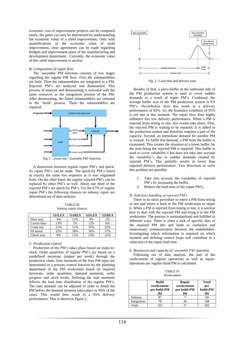
114

economic cost of improvement projects can be computed

easily, the gains can only be determined by understanding

the economic value of a yield improvement. Only with

quantifications of the economic value of yield

improvement, clear agreements can be made regarding

budgets and improvement plans of the manufacturing and

development department. Currently, the economic value

of this yield improvement is unclear.

B. Composition of repair flow

The ‘assemble PM’-function consists of two stages

regarding the regular PM flow. First the subassemblies

are built. Then the subassemblies are integrated to a PM.

Rejected PM’s are analyzed and dismounted. This

process of analysis and dismounting is executed with the

same resources as the integration process of the PM.

After dismounting, the failed subassemblies are returned

to the ‘build’ process. There the subassemblies are

repaired.

Fig. 1 - Zoom into ‘Assemble PM’-function

A distinction between regular repair PM’s and quick-

fix repair PM’s can be made. The quick-fix PM’s return

in exactly the same test sequence as it was originated

from. On the other hand, the regular rejected PM’s can be

replaced by other PM’s as well. About one third of the

rejected PM’s are quick-fix PM’s. For the 67% of regular

repair PM’s the following chances on subassy repair are

determined out of data analysis.

TABLE III

Subassy repair chances

311LEX 311REX 321LEX 321REX

Hose assy 4% 11% 9% 2%

Carrier base 13% 5% 12% 6%

Crash rim 21% 11% 35% 22%

SS motor 25% 58% 56% 37%

Chuck assy 8% 11% 23% 22%

C. Production control

Production of the PM’s takes place based on make-to-

stock. Order quantities of regular PM’s are based on a

predefined moverate (output per week) through the

production chain. Start moments of the four PM types are

determined in a process control function by the planning

department of the PM workcenter based on required

moverate, order quantities, demand moments, order

progress and stock levels. Defining the start moments

follows the lead time distribution of the regular PM’s.

The start moment can be adjusted in order to finish the

PM before the demand moment takes place in 95% of the

cases. This would then result in a 95% delivery

performance. This is shown in figure 2.

Fig. 2 - Lead time and delivery time

Besides of that, a piece-buffer at the outbound side of

the PM production system is used to cover sudden

demands as a result of repair PM’s. Combined, the

average buffer size of the PM production system is 9.9

PM’s. Nevertheless does this result in a delivery

performance of 82%. So, the boundary condition of 95%

is not met at this moment. The repair flow does highly

influence this low delivery performance. When a PM is

rejected from testrig or test, two events take place. First,

the rejected PM is waiting to be repaired. It is added to

the production system and therefore requires a part of the

capacity. Second, an immediate demand for another PM

is created. To fulfill this demand, a PM from the buffer is

consumed. This creates the situation of a lower buffer for

the time being the rejected PM is repaired. This buffer is

used to cover variability’s but does not take into account

the variability’s due to sudden demands created by

rejected PM’s. This partially results in lower than

required delivery performance. Two directions to solve

this problem are possible:

1. Take into account the variability of rejected

PM’s by increasing the buffer.

2. Reduce the lead-time of the repair PM’s.

D. Indistinct handling of rejected PM’s

There is no strict procedure to reject a PM from testrig

or test and return it back to the PM workcenter to repair

it. When a PM is rejected from testrig or test, it is unclear

how to deal with the rejected PM and bring it to the PM

workcenter. The process is unstandardized and fulfilled in

different ways. There is often a lack of specific data of

the repaired PM this and leads to confusion and

unnecessary communication between the stakeholders.

Investigating which information is required on which

moment and defining control loops will contribute to a

reduction of the repair lead time.

E. Resources and capacity of ‘assemble PM’-function

Following out of data analysis, the part of the

workcontent of regular operations as well as repair-

operations per regular build PM is calculated.

TABLE IV

Workcontent

Build

workcontent

per build-PM

[h]

Repair

workcontent

per build-PM

[h]

Total

per

build-PM

[h]

Subassy 87 7 94

Integration 78 30 108

Total 165 37 202

build

analyze and dismountrejected PM

carrier

base

crash rim

integrate

chuck assy

SS motor

PM

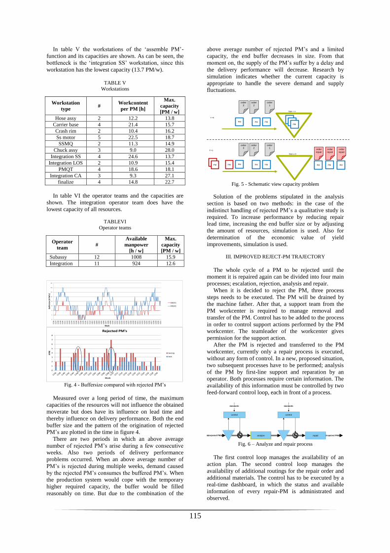
115

In table V the workstations of the ‘assemble PM’-

function and its capacities are shown. As can be seen, the

bottleneck is the ‘integration SS’ workstation, since this

workstation has the lowest capacity (13.7 PM/w).

TABLE V

Workstations

Workstation

type #

Workcontent

per PM [h]

Max.

capacity

[PM / w]

Hose assy 2 12.2 13.8

Carrier base 4 21.4 15.7

Crash rim 2 10.4 16.2

Ss motor 5 22.5 18.7

SSMQ 2 11.3 14.9

Chuck assy 3 9.0 28.0

Integration SS 4 24.6 13.7

Integration LOS 2 10.9 15.4

PMQT 4 18.6 18.1

Integration CA 3 9.3 27.1

finalize 4 14.8 22.7

In table VI the operator teams and the capacities are

shown. The integration operator team does have the

lowest capacity of all resources.

TABLEVI

Operator teams

Operator

team #

Available

manpower

[h / w]

Max.

capacity

[PM / w]

Subassy 12 1008 15.9

Integration 11 924 12.6

Fig. 4 - Buffersize compared with rejected PM’s

Measured over a long period of time, the maximum

capacities of the resources will not influence the obtained

moverate but does have its influence on lead time and

thereby influence on delivery performance. Both the end

buffer size and the pattern of the origination of rejected

PM’s are plotted in the time in figure 4.

There are two periods in which an above average

number of rejected PM’s arise during a few consecutive

weeks. Also two periods of delivery performance

problems occurred. When an above average number of

PM’s is rejected during multiple weeks, demand caused

by the rejected PM’s consumes the buffered PM’s. When

the production system would cope with the temporary

higher required capacity, the buffer would be filled

reasonably on time. But due to the combination of the

above average number of rejected PM’s and a limited

capacity, the end buffer decreases in size. From that

moment on, the supply of the PM’s suffer by a delay and

the delivery performance will decrease. Research by

simulation indicates whether the current capacity is

appropriate to handle the severe demand and supply

fluctuations.

Fig. 5 - Schematic view capacity problem

Solution of the problems stipulated in the analysis

section is based on two methods: in the case of the

indistinct handling of rejected PM’s a qualitative study is

required. To increase performance by reducing repair

lead time, increasing the end buffer size or by adjusting

the amount of resources, simulation is used. Also for

determination of the economic value of yield

improvements, simulation is used.

III. IMPROVED REJECT-PM TRAJECTORY

The whole cycle of a PM to be rejected until the

moment it is repaired again can be divided into four main

processes; escalation, rejection, analysis and repair.

When it is decided to reject the PM, three process

steps needs to be executed. The PM will be drained by

the machine father. After that, a support team from the

PM workcenter is required to manage removal and

transfer of the PM. Control has to be added to the process

in order to control support actions performed by the PM

workcenter. The teamleader of the workcenter gives

permission for the support action.

After the PM is rejected and transferred to the PM

workcenter, currently only a repair process is executed,

without any form of control. In a new, proposed situation,

two subsequent processes have to be performed; analysis

of the PM by first-line support and reparation by an

operator. Both processes require certain information. The

availability of this information must be controlled by two

feed-forward control loop, each in front of a process.

Fig. 6 – Analyze and repair process

The first control loop manages the availability of an

action plan. The second control loop manages the

availability of additional routings for the repair order and

additional materials. The control has to be executed by a

real-time dashboard, in which the status and available

information of every repair-PM is administrated and

observed.

0

2

4

6

8

10

12

14

16

11

36

11

37

11

38

11

39

11

40

11

41

11

42

11

43

11

44

11

45

11

46

11

47

11

48

11

49

11

50

11

51

11

52

12

01

12

02

12

03

12

04

12

05

12

06

12

07

12

08

12

09

12

10

12

11

12

12

12

13

12

14

12

15

12

16

12

17

12

18

12

19

12

20

12

21

12

22

12

23

12

24

12

25

12

26

12

27

12

28

12

29

12

30

12

31

Bu

ffe

rsiz

e [

# P

M's

]

Week

Mk311

Mk321

0

1

2

3

4

5

6

7

8

# PM

Week

Rejected PM's

testrig

test

T = 0

PM

order

3

PM PM

order

2

order

1

T = 1

PM

order

repair

PM

PM

PM

PM PM PM

order

repair

order

repair

PM

order

3

PM PM

order

2

order

1

PM

PM

Size = n

Size = 0

repair repaired PManalyzerejected PM

controlcontrol

standards standards

116

IV. SIMULATION

A. Experimental design

Experiments will be executed based on multi-level

experimental designs, in order to fully understand

solution spaces.

In order to investigate influences of repair lead time

off-line repair scenarios are executed. To investigate

influences of workstation capacity, scenarios with an

increase in workstations are executed.

TABLE VII Scenarios

Current in-line repair Off-line repair

Current # of

workstations

Scenario 1

(4x int. SS)

Scenario 3

(3x rep. stations)

Current # of

workstations

+ 1

Scenario 2

(5x int. SS)

Scenario 4

(4x rep. stations)

Every scenario two parameters are altered; the start

moment (in days before the demand moment) is altered

from 18 days until 32 days and the integration operator

number is altered from 10 until 15 operators. Buffersize

is changed by the start moment. In total 90 experiments

per scenario are executed. Every experiment is run with

20 observations.

To determine the economic value of a yield loss

improvement, scenario 1 is executed with current yield

(68%), the aimed yield (88%) and 100% yield.

B. Simulation model

Simulations runs equals the period of one year, with a

ramp-up of 100 days. The simulation model is designed

by the descriptions given below:

9) There’s a set of workstationgroups containing

workstations of the same kind.

10) PM-orders contain suborders.

11) Suborders, containing an assemblyplan, are executed

on a workstation of a workstationgroup.

12) Every workstation in the same workstationgroup

contains the same set of assemblyplans.

13) The assemblyplans contain a table with several

sequential operation steps and information regarding

a-times, b-chances, b-duration, successors, required

service, etc.

14) Every operation step has its own process time. This

process time is defined out of the input given for this

process step from the table.

15) The routing of PM-orders for build PM’s is identical

for each order. The routing of PM-orders between

the workstationgroups for repair PM’s may vary for

each PM-order.

Fig. 7 – Schematic view of PM flow

C. Cost function

The cost function used to determine variable costs per

PM is based on three elements:

--𝐸𝑞. 1 𝐶𝑡𝑜𝑡𝑎𝑙 = 𝐶𝑙𝑎𝑏𝑜𝑟 + 𝐶𝑐𝑎𝑝𝑖𝑡𝑎𝑙 + 𝐶𝑠𝑐𝑟𝑎𝑝

The labor costs are calculated as follows:

--𝐸𝑞. 2 𝐶𝑙𝑎𝑏𝑜𝑟 = 𝑊𝑖𝑛𝑡 + 𝑊𝑠𝑢𝑏 + 𝑊𝑟𝑒𝑝 ∗ 𝑐𝑙𝑎𝑏𝑜𝑟 ∗ 𝐻

Where [W] is the amount of operators, [c] the costs of

labor per hour (46 euro) and [H] the factory-hours per

year (84 hours/week *52 weeks/year). The capital costs

are calculated as follows:

-𝐸𝑞. 3 𝐶𝑐𝑎𝑝𝑖𝑡𝑎𝑙 = 𝐿𝑇 + 𝐵𝑇

365∗ 𝑊𝐴𝐶𝐶 ∗ 𝑐𝑃𝑀

𝑛

𝑥=1

Where [LT] is the average lead-time, [BT] is the

average buffer time, [WACC] is the weighted average

cost of capital (8%) and [c] is the volume purchase costs

of a PM (823000 euro). The scrap costs are calculated as

follows:

-𝐸𝑞. 4 𝐶𝑠𝑐𝑟𝑎𝑝 = 𝑐𝑠𝑐𝑟𝑎𝑝

𝑛

𝑥=1

Where [c] is the average scrap cost per repair-PM

(4139 euro). To calculate the total average costs per PM,

the total costs are divided by the total amount of regular

PM’s.

D. Verification and validation

The simulation model is verified based on

visualization, tracing and calculations. Calculations are

made regarding lead times, occupancy rates, yield and

costs. Deviations up to 1.5% were noticed. This shows

that the model, regarding of the small deviations, works

as intended.

The simulation model is also validated. This is

executed regarding operator amount, lead time of build

PM’s, buffer time and delivery performance. The model

is validated with deviations up to 16%.

E. Confidence analysis

A confidence analysis is executed to be able to

quantify the quality of the experiments as a result of the

amount of observations per experiment. The 95%

confidence intervals of the variable costs and the delivery

performance will be calculated. The amount of samples is

lower than 30, so according to [Richard I. Levin, 1978]

the t-distribution is required. The t-value for a 95%

confidence interval and a sample size of 20 is 2.093. The

95% confidence interval is calculated as follows:

𝐸𝑞. 5 0.95 = 𝑃 𝑋 − 𝑡 ∗𝜎

𝑛< 𝜇 < 𝑋 + 𝑡 ∗

𝜎

𝑛

Where [t] is the student’s t-distribution value, [𝑋 ] is

the sample mean, [n] is the sample size and [σ] is the

sample standard deviation.

The confidence intervals of all experiments are

determined. This results in the conclusion that the

117

confidence intervals of all experiments are smaller than

the determined deviations of the validation. Therefore it

is concluded that a number of 20 observations per

experiment is sufficient.

V. RESULTS

A. AS-IS

The current configuration of the workcenter is the

situation of 11 integration operators in scenario 1. The

data points are the result of a low start moment (lower

left corner) up to an increased start moment (upper right

corner). In a situation of 81% (current) delivery

performance the costs are equal to 18883 euro. 95%

delivery performance will not be met in this

configuration.

B. Increasing delivery performance

All output values of the simulation experiments of

scenario 1 are shown in figure 9. Delivery performances

Fig. 8 – AS-IS configuration

lower than 77% leads to lower costs in the 11 operator

configuration than in the 12 operator configuration.

Higher delivery performance leads to the opposite. The

11, 12 and 13 operator configurations do have almost

equal performance curves. The 10, 14 and 15 operator

configurations explicitly underperform. A low number of

operators lead to high occupancy rates. This results in

high lead-times. Due to high lead-times, delivery

performance decreases. Opposite, a high number of

operators results in low lead-times and thus a high

delivery performance. But there is more available labor,

which results in increasing labor-costs.

Fig. 9 – AS-IS configuration

Out of all four scenarios the best performing scenario

is selected. Scenario 2 results in the lowest costs with a

delivery performance of more than 95%. These costs are

19475 euro. This is with 5 ‘int. SS’ workstations, 13

integration operators and a start moment of 25 days. It

must be remarked that the best performing configurations

of all four scenarios have a relative small difference

regarding costs.

C. Robustness

To investigate robustness of the above conclusion,

results of the confidence analysis are used. There’s

searched for configurations which do perform lower than

95% delivery performance, but are close to the best

performing configuration. From these configurations the

confidence intervals are shown in figure 10 and figure

11.From figure 10 it is concluded that there is no

statistical significant difference between the four

scenarios near the 95% delivery performance level. From

figure 11 it is concluded that no there is no statistical

significant difference between the two operator

configurations of scenario 1 near the 95% delivery

performance level. Therefore no robust recommendation

can be done regarding the production structure, the

number of workstations and the number of operators.

Fig. 10 – Confidence intervals of configurations of multiple

scenarios

Fig. 11 – Confidence intervals of multiple configurations of the

same scenario

D. Rule-of-thumb occupancy rate

There has to be searched for an alternative

recommendation. In table VIII the occupancy rates of the

integration operator teams are shown of the best

performing configurations of all four scenarios. In the

utmost right column also the occupancy rates of the

second best configuration is shown.

TABLE VIII

Occupancy rates

OR of optimal

configuration

OR of nearly optimal

configuration

Sc.1:

13 – 12 oper. 73% 79%

Sc.2:

13 – 12 oper. 74% 80%

Sc. 3:

12 – 13 oper. 82% 74%

Sc. 4:

12 – 13 oper. 81% 74%

With 95% delivery performance on average the

occupancy rate is 78%. It can be concluded that the

40%

50%

60%

70%

80%

90%

100%

17000 17500 18000 18500 19000 19500 20000 20500 21000

De

live

ry p

erf

orm

an

ce [

%]


Scenario 1, 11 int. operators

18

32

....

....

start moment

40%

50%

60%

70%

80%

90%

100%

17000 18000 19000 20000 21000 22000 23000

De

live

ry p

erf

orm

ance

[%

]


Scenario 1

10 int. operators

11 int. operators

12 int. operators

13 int. operators

14 int. operators

15 int. operators

0.93

0.94

0.95

0.96

0.97

0.98

0.99

1

19000 19200 19400 19600 19800 20000

Del

iver

y pe

rfo

rman

ce [

%]


Confidence analysis

Scenario 2, 13 operators, start 25(best performing)Scenario 1, 12 operators, start 27



0.93

0.94

0.95

0.96

0.97

0.98

0.99

1

19000 19500 20000 20500 21000

Del

iver

y pe

rfor

man

ce [

%]


Confidence analysis

scenario 1, 13 operators, start 28(best performing)

scenario 1, 12 operators, start 29

118

production system has to be equipped with operator

teams which meet an occupancy rate of 78±5%.

E. Reducing yield-loss

There has to be searched for an alternative way of cost

reduction since delivery performance improvements do

not lead to large cost reductions. Therefore the same

configurations for the experiments are used as in scenario

1 but the yield is altered from 68% to 88% and 100%

yield. This is shown in figure 12.

The costs breakdowns of the three yield levels are

shown in figure 13. The costs of the best performing

configuration of the ‘yield 88%’ scenario decreases

largely in comparison to the best performing

configuration of scenario 1. Costs are further decreased

when increasing yield to 100%. Costs are reduced on all

four costs aspects, as was expected.

Fig. 12 –Scenario 1, respectively yield 100%, yield 88% and

yield 68%

Fig. 13 –Cost breakdown of scenario 1: yield 68%, yield 88%

and yield 100%

It can be concluded that, although workcontent only

increased with about 25% due to the yield loss of 32% (as

stipulated in chapter 6), the total variable costs increases

with a percentage of about (20152-13831)/13831 = 45%.

Thus, yield loss does not only lead to increasing labor,

but also substantially negative influence the capital costs

and scrap costs.

The economic value of a yield improvement to 88%

can now easily be calculated. The economic value of a

yield improvement from 68% to 88% results in a yearly

financial benefit of 1741k euro when an average

moverate of 7.4 regular PM’s per week takes place. A

yearly financial benefit of 941k euro takes place with an

average moverate of 4 regular PM’s per week. A reduced

moverate might occur when ASML faces an economic

downturn.

F. Rule-of-thumb startmoment

In every executed scenario the performance of the

production system is optimal with an occupancy rate of

integration operators of 78±5%. This rule-of-thumb gives

information about the resources of the production system.

But to reach a delivery performance of 95%, another rule

is required, which gives information about the production

control. A rule-of-thumb can be defined for the relation

between start moment and yield loss. The startmoments

of the three yield loss scenarios are plotted in figure 14.

The startmoment needs to be increased linearly (from a

constant value of 17 days in the case of 100% yield) with

the yield loss in order to reach a delivery performance of

95%.

Besides of this relation, it is evident that the

startmoment has to be scaled to the workcontent if this

workcontent changes. The prerequisites for this scaling

are that the ratio of workcontent between regular and

repair operations must remain unchanged. Also the

distribution of a-time and b-time must remain unchanged.

Third, the resources have to keep the same occupancy

rates.

Fig. 14 –Startmoments at different yield-losses

Taking these relations into account, the following rule-

of-thumb can be formulated.

𝐸𝑞. 6 𝑠𝑡𝑎𝑟𝑡𝑚𝑜𝑚𝑒𝑛𝑡 = a ∗ 𝑦𝑖𝑒𝑙𝑑𝑙𝑜𝑠𝑠 + 𝑏 ∗𝑊

𝑊𝐴𝑆−𝐼𝑆

Where the startmoment is defined in days, a is a

constant of value 34, yieldloss is expressed in [%], b is a

constant of value 17, W is the workcontent and WAS-IS is

the current workcontent (202 hours).

VI. DISCUSSION

Although there is no statistically significant difference

noticeable between multiple scenarios in order to meet

the moverate, costs and delivery performance

requirements, there are sound rule-of-thumbs defined

which still gives the possibilities to determine the optimal

configuration. Besides of that, the system is improved on

a qualitative base, which gives control over the repair-

PM’s. Also, quantifications of economic gains are made

when improving the current yield from 68% to 88%.

Further research should be deployed regarding a

varying startmoment. Also additional research is required

to be able to extend the occupancy rate rule-of-thumb to

workstations.

REFERENCES

1. Bohn, R.E. & Terwiesch, C. (1999). The economics of yield-driven processes. Journal of Operations

Management 18 (1999) 41-59

2. Levin, R. I. (1978). Statistics for management. Englewood Cliffs, N.J., USA: Prentice-Hall Inc

40%

50%

60%

70%

80%

90%

100%

13000 14000 15000 16000 17000 18000 19000 20000 21000 22000 23000

De

live

ry p

erf

orm

ance

[%

]


Scenario 1: yield 68%, yield 88%, yield 100%

















0

5000

10000

15000

20000

25000

Scenario 1, 13 operators, startmoment 28(DP=95%)



Co

sts

[eu

ro]

Scrap costs per PM



Laborcosts per PM

10

15

20

25

30

35

0% 4% 8% 12% 16% 20% 24% 28% 32% 36%

Star

t m

om

ent

[day

s]

Yield loss [%]

start

34x+17

119

Appendix B–Swimming lane reject PM flow

Part 1: escalation flow and reject flow

120

Part 2: return flow and analyze /repair flow

121

Appendix C – Dashboard of rejected PM’s

122

Appendix D – Scrap

Scrap costs needs to be taken into account as it is one of the cost aspects of yield loss. When the

yield loss becomes reduced, the cost reduction is calculated to give insight in the economic value. The

variable costs of labor and WIP doesn‟t give a complete view on the economic value of a yield change

without the costs of scrap.

Out of data analysis, the following data is deployed.

The scrap costs of 4139 euro per rejected PM are a weighted average of the scrap costs of both the

regular repair PM as well as the quick fix repair PM.

order typeaverage scrap

costs per order

chance of repair

orders per

rejectPM [%]

scrap costs

per rejectPM

hose assy 3092 4% 129

carrier base 1753 6% 103

crash rim 745 16% 120

ss motor 1720 30% 517

chuck assy 954 12% 116

integration 3154 100% 3154

total 4139

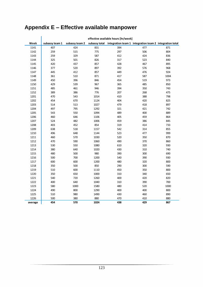
123

Appendix E – Effective available manpower

Week subassy team 1 subassy team 2 subassy total integration team 1 integration team 2 integration total

1141 407 424 831 394 477 871

1142 259 515 775 297 506 804

1143 259 329 587 412 424 836

1144 325 501 826 317 523 840

1145 420 437 857 428 467 895

1146 377 520 897 392 576 968

1147 445 412 857 449 476 924

1148 361 510 871 417 587 1004

1149 450 396 846 454 519 973

1150 429 539 967 365 485 850

1151 485 461 946 394 350 743

1152 389 386 776 207 268 475

1201 470 543 1014 410 388 798

1202 454 670 1124 404 420 825

1203 514 513 1027 479 418 897

1204 497 795 1292 321 421 742

1205 543 550 1094 489 400 889

1206 460 646 1106 405 459 864

1207 524 482 1006 459 386 845

1208 403 452 854 319 414 733

1209 638 518 1157 542 314 855

1210 496 648 1144 523 477 999

1211 460 570 1030 520 350 870

1212 470 590 1060 490 370 860

1213 530 550 1080 610 320 930

1214 380 640 1020 430 310 740

1215 480 500 980 390 300 690

1216 500 700 1200 540 390 930

1217 600 600 1200 480 320 800

1218 350 500 850 290 300 590

1219 510 600 1110 450 350 800

1220 350 650 1000 310 340 650

1221 540 720 1260 400 420 820

1222 400 640 1040 310 390 700

1223 580 1000 1580 480 520 1000

1224 490 800 1290 400 400 800

1225 510 980 1490 430 460 890

1226 500 380 880 470 410 880

average 454 570 1024 438 429 867

effective available hours [hr/week]

124

Appendix F – Disturbance management Disturbances are often occurring during production of the PM‟s. Typically, one time unit of production

results in two time units of disturbance resolution. The disturbances are subdivided into eight

categories.

• B1 – Material not available

• B2 – Material not usable (Quality issue)

• B3 – Workmanship issue

• B4 – Tooling issue

• B5 – Facility issue

• B6 – Material documentation / packaging is NOK

• B7 – Procedure issue

• B8 – Technical issue

Figure 13 gives an indication of the duration per disturbance category. Most of the disturbances are

logged as category B2. The subcategory „B2 – other‟ takes 4500 hours during the third and fourth

quarter of 2011.

Disturbance resolution

Figure 59 - Total disturbance duration in period 201126 - 201152

125

At the moment a disturbance occurs, the operator creates a Disturbance Notification; a DN. the

operator has 30 minutes to solve it with prescribed methods, so-called fish-bones. When he is not

able to solve the disturbance, first-line support is requested to support with the problem. The first-line

support is present in the workcenter. According to the disturbance category a material handler (MH),

a Technical OPerationS coordinator (TOPS) or a Means&Methods employee (MM) is requested. The

first-line support tries to solve the disturbance. When he won‟t succeed within a prescribed time, the

second-line support is requested by the first-line support. This second-line support has more

knowledge on product and procedures. Second-line support consists of Production Planning (PP),

Material Quality department (MQ) or Manufacturing Engineering (ME). But when second-line support

is unable to solve the disturbance either, third-line support is activated. The third-line support

consists of program management (PRO), supply chain engineering (SCE) or development &

engineering (D&E). This escalation process is shown in Figure 60.

Figure 60 - escalation flow

Figure 61 - 'German flag'

The severity of the disturbance is also categorized. Right from the beginning of the disturbance an

immediate escalation to higher level supports might be necessary. The operator decides on this with

126

the so-called „German Flag‟. This „German flag‟ shows a severity scale, criteria and escalation actions.

In this way, ASML is able to decrease the reaction time to the right department. Also in this way

safety issue prevention is integrally picked up by the disturbance system.

Disturbance containment

In the previous section, the process structure regarding disturbance resolution is explained. But to

prevent keep solving the same disturbances over and over again, also a system of disturbance

containment is necessary.

Containment of disturbances consists of a process control and a function control over the regular

„assemble‟ process. From the regular „assemble‟ process material with a disturbance flows to the

disturbance resolution process. There the disturbance will be handled. The disturbances and the

solutions are logged in the ERP system. These DN loggings are categorized and listed. On execution

level, these DNs are contained by the PCS (Problem, Cause and Solution) methodology. Process

control over the execution is used to improve on a small scale and in a relative short timespan

measure measure

comparecontrol

intervene

initiate evaluate

DN/MN lists

DN reports

SAPIR action

list

DRB/GL

TL

solution for

root cause

DN logging

analysis DNs

CIP

PIT

aspiration sheet

targets

ME

SAPIR action

progress

solve

assemblematerial

material with

disturbance

material with

solved disturbance

PM

Figure 62 - Control over the disturbance aspect

127

(weeks). The logged DNs are analyzed by the DRB (Disturbance Review Board). This Board proposes

a PIT (Performance Improvement Team) for a certain disturbance type. After agree of forming the

PIT, the PIT starts to improve on the disturbance type via the PCCSIM (Problem, Containment, Cause,

Solution, Implementation and Monitor) methodology.

The function control is used to implement solutions on a large scale and in a large timespan

(months). The logged DNs are listed and evaluated by ME. The analysis is used to make reports and

used for proposing an action list. This action list is executed by using the SAPIR (Scope, Action, Plan,

Implement, Results) methodology. The PIT takes care to implement the proposed actions. The

progress in the SAPIR lists is measured and discussed in the CIP (Continuous Improvement Process).

128

Appendix G - Disturbance duration In this appendix the disturbance times are determined.

Because the data of the disturbance times is measured from a real start time to a real end time, the

shift calendar is not taken into account. During night, there is no production, but it is measured in the

b-time data as disturbance time. These data is corrected for the current two shift model. The

disturbance time dataset do have values between the interval of 10 minutes disturbance duration and

one week disturbance duration. It is assumed that data with duration smaller than 10 minutes the

effect is negligible while the chance of being a wrong logging is high. Considering the way of working

within the factory it is impossible to make a DN, inform the first line support, diagnose the problem,

solve the problem and close the DN all within the time span of 10 minutes. Also, disturbances taking

more than one week to be closed are considered as extreme loggings. In the case there is a material

missing, the PM is removed from the workstation and stored during the disturbance time. When

stored but still noted as a disturbance, the PM doesn‟t have its influence on the production process.

Therefore it is assumed that these extreme loggings are invalid.

Furthermore it is important to notice differences between disturbance times of sub-assy orders and

integration orders. As explained, the production of the PM consists of the production of 5 subassy‟s

and the integration of these subassy‟s. So, in total there are six types of orders. The disturbance

notifications are separated to these six types. After that, the amount of occurrence of the duration of

the notifications is normalized to the total amount of disturbance notifications per order type. This is

done to be able to compare the distributions of the different types to each other. Due to the small

dataset of notifications of the hose assy orders, the crashrim orders and the chuck assy orders, this

data is not evaluated. In figure… the data of the shortstroke orders, the carrier base orders and the

integration orders is shown (period of week 1126 to 1152). It can be concluded that there is a strong

similarity in all three of the graphs. Therefore it is assumed that it is possible to use one distribution

extracted from the whole dataset of notifications for further calculations.

129

Figure 63 - Disturbance duration distribution of order types

The disturbance times do have a strongly lognormal distributed occurrence, as is shown in figure 63

of the order types and in figure 64 using the data of all order types as a whole.

Figure 64 - Disturbance duration distribution

130

To calculate the properties of this lognormal distribution (mu, sigma) the average and the standard

deviation needs to be measured. These parameters do have the following values:

E[X] = 5.50 hours

s.d.[X] = 9.44 hours

The variance Var[X] is the square root of the standard deviation s.d.[X]:

s. d. [X]2 = Var[X]

Var X = 9.442 = 89.19

With the equations below and by knowing the expected value and the variance the parameters μ

andσ can be obtained:

μ = ln E X −1

2∗ ln 1 +

𝑉𝑎𝑟[𝑋]

(𝐸 𝑋 )2

σ2 = ln 1 +𝑉𝑎𝑟[𝑋]

(𝐸 𝑋 )2

Using these equations gives the values for parameters μ andσ:

μ = 1.018

𝜎2 = 1.373

131

Appendix H - Initialization time of the model It is assumed that the average throughput time of a PM will not be larger than 20 days. The

consolidated yield loss is measured to be 32%. So the average regular build PM has a chance of 32%

to become a repair PM. As one can understand, it takes some time before the model runs with a

balanced output. With an inter arrival time of 11.33 hours, the moverate of new PM‟s is 84/11.33 =

7.44 PM‟s per week. On average, after the assumed throughput time of 20 days, the moverate will be

increased by a set of repair PM‟s of 7.44*0.32 = 2.38 repair PM‟s. After two times the throughput

time (40 days), 7.44 new and 2.38 repair PMs will be accompanied by 2.38*0.32 = 0.62 repair PM‟s.

This continues until a balanced moverate will be reached. As can be seen in figure .., after the fourth

generation of repair PM‟s, there‟s hardly any increase in average moverate anymore. The time needed

to reach the moverate of the fourth generation is equal to 20*5 = 100 days. Therefore a ramp-up

time of 100 days will be sufficient.

Figure 65 - Moverate ramp-up calculation

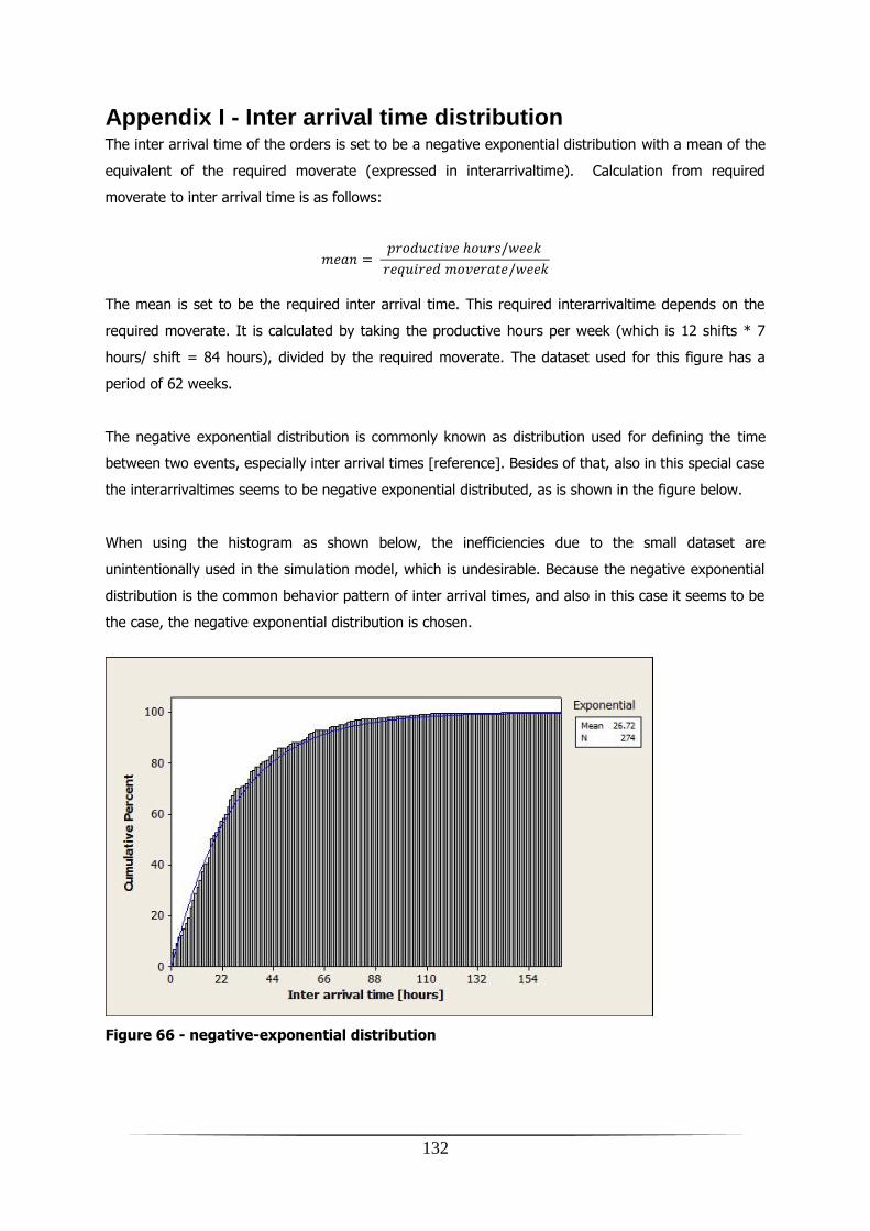
132

Appendix I - Inter arrival time distribution The inter arrival time of the orders is set to be a negative exponential distribution with a mean of the

equivalent of the required moverate (expressed in interarrivaltime). Calculation from required

moverate to inter arrival time is as follows:

𝑚𝑒𝑎𝑛 = 𝑝𝑟𝑜𝑑𝑢𝑐𝑡𝑖𝑣𝑒 𝑕𝑜𝑢𝑟𝑠/𝑤𝑒𝑒𝑘

𝑟𝑒𝑞𝑢𝑖𝑟𝑒𝑑 𝑚𝑜𝑣𝑒𝑟𝑎𝑡𝑒/𝑤𝑒𝑒𝑘

The mean is set to be the required inter arrival time. This required interarrivaltime depends on the

required moverate. It is calculated by taking the productive hours per week (which is 12 shifts * 7

hours/ shift = 84 hours), divided by the required moverate. The dataset used for this figure has a

period of 62 weeks.

The negative exponential distribution is commonly known as distribution used for defining the time

between two events, especially inter arrival times [reference]. Besides of that, also in this special case

the interarrivaltimes seems to be negative exponential distributed, as is shown in the figure below.

When using the histogram as shown below, the inefficiencies due to the small dataset are

unintentionally used in the simulation model, which is undesirable. Because the negative exponential

distribution is the common behavior pattern of inter arrival times, and also in this case it seems to be

the case, the negative exponential distribution is chosen.

Figure 66 - negative-exponential distribution

133

Appendix J – input of the simulation model

Table 28 - hose assy operations

Table 29 - carrier base operations

ID Workstation Task name A-Time [h] FailureChance [%] Avg. Failure Time [h] S.D. Failure Time [h] # Operators Materials

1 hose assy 01_A__ASSEMBLE HOSE ASSY LEX _ 6.50 14% 5.50 9.44 1

2 hose assy CHECKPOINTS CB-HA-CR 0.50 6% 5.50 9.44 1

3 hose assy 02_A__LEAKTESTING HOSE ASSY LEX/REX _ 3.50 7% 5.50 9.44 1

4 hose assy Configuration check 0.25 0% 5.50 9.44 1


9 carrier base 01_A__PREPARING THE CARRIER STRUCTURE _ 0.50 5% 5.50 9.44 1

10 carrier base 01_A__ASSEMBLE E-BOX [LEX] [MK3.2] _ 0.67 18% 5.50 9.44 1

11 carrier base Install Bottom PCA + LEVI Sensors (LEX) 1.00 8% 5.50 9.44 1

12 carrier base Install Accelero Sensors (LEX) 0.50 0% 5.50 9.44 1

13 carrier base Creation Deviation Notice - Conf. Man 0.17 0% 5.50 9.44 1

14 carrier base 01_A__MOUNT PE SET [LEX] [MK3.2] _ 0.33 0% 5.50 9.44 1

15 carrier base 01_A__MOUNT POWER CABLES [LEX] [MK3.2] _ 1.00 8% 5.50 9.44 1

16 carrier base CHECKPOINTS CB-HA-CR 0.17 6% 5.50 9.44 1

17 carrier base 02_A__PLACE HOSE ASSEMBLY LEX _ 2.00 12% 5.50 9.44 1


19 carrier base 02_A__MOUNT SLAB PCA [LEX] [MK3.2] _ 1.00 7% 5.50 9.44 1

20 carrier base 02_A__PLACE APE INTERFERENCE PLATE LEX _ 0.50 2% 5.50 9.44 1


22 carrier base Install Encoder Remote Box (LEX) 0.33 7% 5.50 9.44 1

23 carrier base Install E-Box Front Assy (LEX 0.75 7% 5.50 9.44 1

24 carrier base 03_A__PLACE E-BOX LEX/REX MK3.2 _ 1.00 6% 5.50 9.44 1


26 carrier base 03_A__PLACE CFC/PPVESSEL LEX/REX _ 0.50 1% 5.50 9.44 1

27 carrier base MOUNT SS2LOS BLOCKS LEX 0.50 5% 5.50 9.44 1


29 carrier base 03_A__CONNECTIVITY TEST _ 0.25 4% 5.50 9.44 1

30 carrier base 03_A__LEVI-Z MEASUREMENT _ 0.67 1% 5.50 9.44 1

31 carrier base 04_A__LEAKTEST LCW/RCW OF THE CARRIER _ 2.17 7% 5.50 9.44 1

32 carrier base 04_A__WI DUMMY ASSY LEX/REX _ 0.50 3% 5.50 9.44 1

134

Table 30 - crash rim operations

Table 31 - short stroke operations


58 crash rim 01_A__PLACE RX-LIMITER,PCA,BRACKETS LEX 2.00 35% 5.50 9.44 1

59 crash rim 01_A__PLACE Z-ENDSTOPS,HOSES,CLAMPS LEX 1.50 16% 5.50 9.44 1

60 crash rim 01_A__PLACE PURGING UNIT AND PPL LEX _ 1.25 6% 5.50 9.44 1

61 crash rim 01_A__EXECUTE PRESSURE TEST CR LEX 1.50 14% 5.50 9.44 1

62 crash rim 01_A__CHECKPOINTS CB-HA-CR _ 0.25 0% 5.50 9.44 1

63 crash rim Configuration check 0.00 0% 5.50 9.44 1


70 SS Configuration check 0.08 0% 5.50 9.44 1

71 SS 01_A__INSPECT AND PREPARE_ 0.75 20% 5.50 9.44 1

72 SS 01_A__Place LCW & RCW hoses LEX_ 1.50 9% 5.50 9.44 1

73 SS 01_A__CHECK WORKMANSHIP BY TOPS_ 0.25 2% 5.50 9.44 1

74 SS PRESURE TEST OF RCW AND LCW LEX/REX 1.67 17% 5.50 9.44 1

75 SS 01_A__MOUNT PE-WIRE-R-LID,..._ 1.67 11% 5.50 9.44 1

76 SS 02_A__HIGH CLEARENCE CHECK LEX/REX_ 1.17 0% 5.50 9.44 1


78 SS 02_A__MOUNT 3X DIFF.SENSOR_ 0.50 0% 5.50 9.44 1

79 SS 02_A__ROUTE POWER CABLES AND HOSES LEX_ 2.50 2% 5.50 9.44 1

80 SS 02_A__ROUTE NTC/PTC WIRES LEX/REX_ 2.00 2% 5.50 9.44 1

81 SS 03_A__MOUNT THE MANIFOLD BLOCKS_ 1.50 5% 5.50 9.44 1


83 SS 03_A__INTEGRATE E-PIN ASSY _ 1.50 16% 5.50 9.44 1

84 SS 03_A__CLEARENCE CHECK SHORT_ 0.50 9% 5.50 9.44 1

85 SS 03_A__FINALIZE SSM_ 0.50 0% 5.50 9.44 1


135

Table 32 - SSMQ operations

Table 33 - chuck assy operations

Table 34 - integrate short stroke operations (1)


129 ssmq SSMQ Instal SSA to SSMQ tool LEX/REX 2.00 10% 5.50 9.44 1

130 ssmq SSMQ Connect PM to PMQT 0.33 4% 5.50 9.44 1

131 ssmq SSMQ Checklist 0.08 0% 5.50 9.44 1

132 ssmq SSMQ SS Motor Temp. and Resistances 0.17 8% 5.50 9.44 1

133 ssmq SSMQ SS Cooling Circuits 0.17 4% 5.50 9.44 1

134 ssmq SSMQ SS 6 DOF Control Functionality 0.17 27% 5.50 9.44 1

135 ssmq SSMQ SS Diff Sensors 0.17 9% 5.50 9.44 1

136 ssmq SSMQ SS Diff Measurement System Cal 0.17 12% 5.50 9.44 1

137 ssmq SSMQ SS Mechanical Range 0.17 1% 5.50 9.44 1

138 ssmq SSMQ SS Endstop Location 0.25 6% 5.50 9.44 1

139 ssmq SSMQ SS Stiffness and Hysteresis 0.17 13% 5.50 9.44 1

140 ssmq SSMQ E Pins 0.17 14% 5.50 9.44 1

141 ssmq SSMQ SS Motor Constants 0.17 4% 5.50 9.44 1

142 ssmq SSMQ Finalize 0.17 1% 5.50 9.44 1

143 ssmq SSMQ DISMOUNT SSA FROM TOOL 0.67 2% 5.50 9.44 1

144 ssmq Configuration check 0.08 0% 5.50 9.44 1


145 chuck assy Unpack and inspect chuck 0.50 29% 5.50 9.44 1

146 chuck assy Perform leakage test 0.33 0% 5.50 9.44 1

147 chuck assy Mount bridgehead Y- & Y+ 1.50 7% 5.50 9.44 1

148 chuck assy GLUE BRIDGE BES HOSE 0.17 0% 5.50 9.44 1

149 chuck assy Fix PCA on chuck sensor brackets 0.75 0% 5.50 9.44 1

150 chuck assy Perform second conductivity test PCA 1.00 2% 5.50 9.44 1

151 chuck assy Mount the encoder heads 1.00 7% 5.50 9.44 1

152 chuck assy Adjust the encoder heads 0.33 0% 5.50 9.44 1

153 chuck assy Finalize chuck assembly 0.33 0% 5.50 9.44 1

154 chuck assy CHECKLIST 0.25 7% 5.50 9.44 1


155 int_SS Configuration check 0.00 0% 5.50 9.44 1 carrier base; crash rim; SS motor

156 int_SS SSM Integration (Calib. Shimming) 6.50 43% 5.50 9.44 1

157 int_SS Check List SSM (Mid Procedure) 0.50 3% 5.50 9.44 1

158 int_SS SSM Integration (Prod. Shimming) 6.50 44% 5.50 9.44 1

136

Table 35 - integrate longstroke operations

Table 36 - integrate short stroke operations

Table 37 - PMQT1 operations


159 int LOS 03_A__CHECKLIST_ 0.50 9% 5.50 9.44 1

160 int LOS 03_A__PLACE COOL PLATES MK3 LEX-REX_ 3.00 31% 5.50 9.44 1

161 int LOS 03_A__PLACE LOS MOTORS LEX - REX MK3_ 3.00 14% 5.50 9.44 1

162 int LOS 04_A__CHECKLIST_ 0.50 1% 5.50 9.44 1

163 int LOS PERFORM LEAK TEST SSM ASSY (REX & LEX) 0.00 2% 5.50 9.44 1


164 int_SS 04_A__LA2LOS ASSY ADJUSTMENT_ 3.50 26% 5.50 9.44 1

165 int_SS 04_A__MOUNT THE DIFF. SENSORS_ 0.75 6% 5.50 9.44 1

166 int_SS CHECK PM FOR CONTAMINATION 0.00 2% 5.50 9.44 1


167 PMQT PMQT Connect PM to PMQT Phase 1 0.33 5% 5.50 9.44 1

168 PMQT PMQT Checklist 0.08 0% 5.50 9.44 1

169 PMQT PMQT Queue 1 Phase 1 0.08 2% 5.50 9.44 1

170 PMQT PMQT LoS Forcers 0.17 3% 5.50 9.44 1

171 PMQT PMQT WT Vacuum (Dummy Restriction) 0.17 5% 5.50 9.44 1

172 PMQT PMQT SS Cooling Circuits 0.17 3% 5.50 9.44 1

173 PMQT PMQT SS 6 DOF Control Functionality 0.17 12% 5.50 9.44 1

174 PMQT PMQT SS Diff Sensors 0.17 11% 5.50 9.44 1

175 PMQT PMQT SS Diff Measurement System Cal 0.17 8% 5.50 9.44 1

176 PMQT PMQT SS Mechanical Range 0.17 0% 5.50 9.44 1

177 PMQT PMQT SS Endstop Location 0.25 1% 5.50 9.44 1

178 PMQT PMQT SS Stiffness and Hysteresis 0.17 4% 5.50 9.44 1

179 PMQT PMQT Pulse Limiter 0.17 0% 5.50 9.44 1

180 PMQT PMQT Check BES and WES 0.17 0% 5.50 9.44 1

181 PMQT PMQT SS Motor Constants 0.17 2% 5.50 9.44 1

182 PMQT PMQT E Pins 0.17 3% 5.50 9.44 1

183 PMQT PMQT LOS Acceleration Sensors 0.17 5% 5.50 9.44 1

184 PMQT PMQT SS Motor Temp. and Resistances 0.17 0% 5.50 9.44 1

185 PMQT PMQT LA_Y Diff Sensors 0.17 1% 5.50 9.44 1

186 PMQT PMQT LA_X Encoder 0.17 3% 5.50 9.44 1

187 PMQT PMQT Purge Hood Temperature Sensors 0.17 1% 5.50 9.44 1

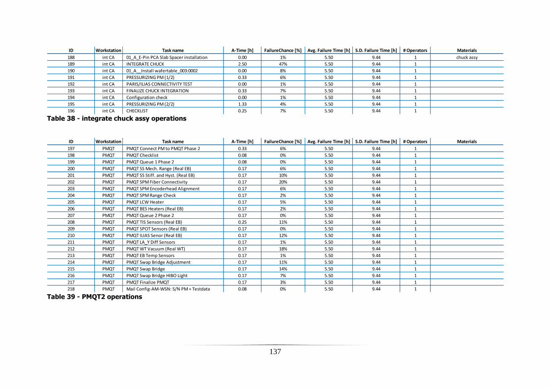
137

Table 38 - integrate chuck assy operations

Table 39 - PMQT2 operations


188 int CA 01_A_E-Pin PCA Slab Spacer installation 0.00 1% 5.50 9.44 1 chuck assy

189 int CA INTEGRATE CHUCK 2.50 47% 5.50 9.44 1

190 int CA 01_A__Install wafertable_003:0002 0.00 8% 5.50 9.44 1

191 int CA PRESSURIZING PM (1/2) 0.33 6% 5.50 9.44 1

192 int CA PARIS/ILIAS CONNECTIVITY TEST 0.00 1% 5.50 9.44 1

193 int CA FINALIZE CHUCK INTEGRATION 0.33 7% 5.50 9.44 1

194 int CA Configuration check 0.00 1% 5.50 9.44 1

195 int CA PRESSURIZING PM (2/2) 1.33 4% 5.50 9.44 1

196 int CA CHECKLIST 0.25 7% 5.50 9.44 1


197 PMQT PMQT Connect PM to PMQT Phase 2 0.33 6% 5.50 9.44 1

198 PMQT PMQT Checklist 0.08 0% 5.50 9.44 1


200 PMQT PMQT SS Mech. Range (Real EB) 0.17 6% 5.50 9.44 1

201 PMQT PMQT SS Stiff. and Hyst. (Real EB) 0.17 10% 5.50 9.44 1

202 PMQT PMQT SPM Fiber Connectivity 0.17 20% 5.50 9.44 1

203 PMQT PMQT SPM Encoderhead Alignment 0.17 6% 5.50 9.44 1

204 PMQT PMQT SPM Range Check 0.17 2% 5.50 9.44 1

205 PMQT PMQT LCW Heater 0.17 5% 5.50 9.44 1

206 PMQT PMQT BES Heaters (Real EB) 0.17 2% 5.50 9.44 1


208 PMQT PMQT TIS Sensors (Real EB) 0.25 11% 5.50 9.44 1

209 PMQT PMQT SPOT Sensors (Real EB) 0.17 0% 5.50 9.44 1

210 PMQT PMQT ILIAS Senor (Real EB) 0.17 12% 5.50 9.44 1

211 PMQT PMQT LA_Y Diff Sensors 0.17 1% 5.50 9.44 1

212 PMQT PMQT WT Vacuum (Real WT) 0.17 18% 5.50 9.44 1

213 PMQT PMQT EB Temp Sensors 0.17 1% 5.50 9.44 1

214 PMQT PMQT Swap Bridge Adjustment 0.17 11% 5.50 9.44 1

215 PMQT PMQT Swap Bridge 0.17 14% 5.50 9.44 1

216 PMQT PMQT Swap Bridge HIBO Light 0.17 7% 5.50 9.44 1

217 PMQT PMQT Finalize PMQT 0.17 3% 5.50 9.44 1

218 PMQT Mail Config-AM-WSN: S/N PM + Testdata 0.08 0% 5.50 9.44 1

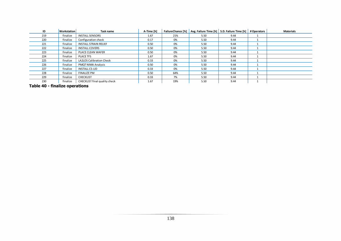
138

Table 40 - finalize operations


219 finalize INSTALL SENSORS 1.67 21% 5.50 9.44 1

220 finalize Configuration check 0.17 0% 5.50 9.44 1

221 finalize INSTALL STRAIN RELIEF 0.50 0% 5.50 9.44 1

222 finalize INSTALL COVERS 0.50 0% 5.50 9.44 1

223 finalize PLACE CLEAN WAFER 0.50 0% 5.50 9.44 1

224 finalize PLACE TFS 1.67 0% 5.50 9.44 1

225 finalize LA2LOS Calibration Check 0.33 0% 5.50 9.44 1

226 finalize PMQT NIMA Analysis 0.50 0% 5.50 9.44 1

227 finalize INSTALL CS-LID 0.33 0% 5.50 9.44 1

228 finalize FINALIZE PM 0.50 64% 5.50 9.44 1

229 finalize CHECKLIST 0.33 7% 5.50 9.44 1

230 finalize CHECKLIST final quality check 1.67 19% 5.50 9.44 1

139

Appendix K – Occupancy rates of workstations

Figure 67 - occupancy rates of workstations of scenario 1…4

Figure 68 - occupancy rates of workstations with increased yield

0.00

0.10

0.20

0.30

0.40

0.50

0.60

0.70

0.80

0.90

1.00

hose_assy cb ss ssmq cr ca int_ss int_los pmqt int_CA finalize repair_int

Occ

up

ancy

rat

e

Workstationgroup

Average of Scenario 1




140

Appendix L – output of the experiments

Table 41 - Scenario 1 (1)

experiment

start

moment

[days]

integration

operators

[#]

subassy

operators

[#]

repair

operators

[#]

output build

[PM/w]

output repair

[PM/w]

output quick

fix [PM/w]

output total

[PM/w]

avg LT build

[days]

avg. LT repair

[days]

avg. LT quick fix

[days]

avg.

buffersize

[# PM]

occ. rate int

operators [%]

occ. rate

subassy

operators [%]

occ. rate

repair

operators [%]

labor costs

per PM

[euro]

capital costs

LT per PM

[euro]

capital costs

BT per PM

[euro]

scrap costs

per PM

[euro]

total costs

per PM

[euro]

delivery

performance

[%]

Exp 01 18 10 12 - 7.33 2.30 1.16 10.79 17.63 14.68 6.73 1.9 94% 68% - 11516 4204 218 1956 17894 43%

Exp 02 18 11 12 - 7.43 2.37 1.17 10.96 14.66 11.68 6.53 2.9 87% 68% - 11876 3497 388 1969 17729 53%

Exp 03 18 12 12 - 7.47 2.38 1.20 11.05 13.59 10.61 6.36 3.5 80% 68% - 12359 3244 491 1986 18079 63%

Exp 04 18 13 12 - 7.48 2.36 1.20 11.03 13.24 10.18 6.15 3.7 74% 68% - 12821 3138 533 1970 18462 66%

Exp 05 18 14 12 - 7.49 2.39 1.19 11.06 13.24 10.23 6.16 3.8 68% 68% - 13362 3150 538 1978 19029 68%

Exp 06 18 15 12 - 7.49 2.39 1.17 11.04 13.25 10.15 6.09 3.6 64% 69% - 13870 3140 520 1966 19496 68%

Exp 07 19 10 12 - 7.37 2.31 1.17 10.85 17.63 14.51 6.83 2.2 95% 68% - 11514 4199 251 1954 17918 47%

Exp 08 19 11 12 - 7.43 2.35 1.18 10.97 14.66 11.60 6.47 3.8 87% 68% - 11923 3494 524 1966 17907 59%

Exp 09 19 12 12 - 7.46 2.38 1.19 11.03 13.67 10.68 6.27 4.3 80% 68% - 12362 3256 638 1980 18236 67%

Exp 10 19 13 12 - 7.53 2.38 1.19 11.09 13.34 10.26 6.19 4.8 74% 68% - 12869 3171 717 1964 18720 73%

Exp 11 19 14 12 - 7.53 2.40 1.19 11.11 13.24 10.15 6.11 4.7 68% 68% - 13392 3149 701 1974 19216 73%

Exp 12 19 15 12 - 7.50 2.38 1.20 11.08 13.21 10.13 6.12 4.7 64% 68% - 13893 3143 708 1978 19722 75%

Exp 13 20 10 12 - 7.31 2.32 1.17 10.80 17.69 14.76 7.02 2.8 94% 68% - 11483 4229 333 1973 18017 50%

Exp 14 20 11 12 - 7.42 2.35 1.18 10.94 14.71 11.77 6.46 4.3 86% 68% - 11875 3504 622 1963 17964 61%

Exp 15 20 12 12 - 7.45 2.39 1.19 11.02 13.58 10.69 6.29 5.0 80% 68% - 12344 3241 747 1983 18316 72%

Exp 16 20 13 12 - 7.45 2.37 1.18 11.00 13.30 10.38 6.17 5.3 74% 68% - 12831 3164 809 1971 18774 75%

Exp 17 20 14 12 - 7.45 2.38 1.18 11.01 13.30 10.28 6.26 5.4 68% 68% - 13352 3159 816 1977 19304 76%

Exp 18 20 15 12 - 7.45 2.38 1.19 11.01 13.28 10.32 6.27 5.3 64% 68% - 13854 3163 799 1984 19799 76%

Exp 19 21 10 12 - 7.31 2.31 1.18 10.80 17.79 14.84 6.77 3.6 94% 68% - 11441 4246 471 1973 18130 58%

Exp 20 21 11 12 - 7.46 2.34 1.18 10.98 14.86 12.02 6.64 5.1 86% 68% - 11865 3553 757 1954 18129 65%

Exp 21 21 12 12 - 7.46 2.39 1.17 11.02 13.61 10.70 6.33 6.2 80% 68% - 12335 3250 964 1978 18527 77%

Exp 22 21 13 12 - 7.53 2.36 1.18 11.07 13.32 10.32 6.07 6.5 73% 68% - 12815 3155 1013 1943 18926 81%

Exp 23 21 14 12 - 7.48 2.37 1.18 11.04 13.32 10.34 6.22 6.2 68% 68% - 13337 3172 964 1967 19440 81%

Exp 24 21 15 12 - 7.52 2.35 1.18 11.04 13.23 10.30 6.14 6.3 64% 68% - 13843 3145 986 1944 19919 82%

Exp 25 22 10 12 - 7.33 2.30 1.16 10.80 17.83 14.92 7.02 3.9 94% 68% - 11420 4259 515 1956 18150 59%

Exp 26 22 11 12 - 7.44 2.35 1.16 10.95 14.72 11.65 6.53 5.9 86% 68% - 11826 3497 891 1951 18165 71%

Exp 27 22 12 12 - 7.48 2.36 1.17 11.01 13.74 10.63 6.34 6.6 80% 69% - 12294 3261 1034 1957 18546 80%

Exp 28 22 13 12 - 7.47 2.41 1.17 11.05 13.42 10.50 6.28 7.1 74% 69% - 12805 3201 1120 1983 19108 84%

Exp 29 22 14 12 - 7.48 2.41 1.16 11.06 13.37 10.37 6.24 7.2 68% 69% - 13335 3182 1134 1975 19627 83%

Exp 30 22 15 12 - 7.51 2.42 1.18 11.10 13.22 10.31 6.05 6.9 64% 69% - 13803 3147 1089 1982 20021 84%

Exp 31 23 10 12 - 7.35 2.34 1.16 10.85 18.00 15.09 7.19 4.4 94% 68% - 11460 4311 606 1968 18345 62%

Exp 32 23 11 12 - 7.46 2.32 1.17 10.96 14.60 11.64 6.55 7.4 86% 68% - 11852 3475 1150 1937 18414 76%

Exp 33 23 12 12 - 7.53 2.36 1.17 11.07 13.60 10.65 6.37 7.8 79% 68% - 12322 3238 1237 1944 18741 85%

Exp 34 23 13 12 - 7.52 2.36 1.19 11.07 13.21 10.17 6.26 8.3 74% 68% - 12834 3138 1330 1955 19257 88%

Exp 35 23 14 12 - 7.49 2.38 1.17 11.05 13.13 10.24 6.15 8.5 68% 68% - 13345 3127 1364 1964 19800 88%

Exp 36 23 15 12 - 7.53 2.40 1.16 11.08 13.18 10.26 6.08 8.5 64% 69% - 13861 3133 1371 1953 20318 89%

Exp 37 24 10 12 - 7.33 2.32 1.15 10.81 17.89 15.05 7.03 5.1 94% 68% - 11416 4286 727 1963 18391 67%

Exp 38 24 11 12 - 7.37 2.35 1.21 10.93 14.72 11.95 6.76 7.7 86% 68% - 11853 3531 1203 1995 18583 78%

Exp 39 24 12 12 - 7.41 2.38 1.19 10.98 13.51 10.67 6.33 8.8 80% 68% - 12352 3230 1422 1989 18993 87%

Exp 40 24 13 12 - 7.45 2.37 1.17 10.99 13.17 10.23 6.21 9.2 73% 68% - 12821 3128 1497 1968 19414 89%

Exp 41 24 14 12 - 7.42 2.39 1.18 10.98 13.09 10.14 6.10 9.2 68% 68% - 13335 3110 1505 1992 19942 91%

Exp 42 24 15 12 - 7.42 2.37 1.16 10.96 13.14 10.22 6.18 9.4 64% 68% - 13875 3129 1538 1975 20516 92%

Exp 43 25 10 12 - 7.33 2.30 1.16 10.78 17.95 15.03 7.08 6.0 94% 68% - 11347 4291 884 1953 18475 71%

Exp 44 25 11 12 - 7.40 2.38 1.18 10.95 14.76 12.05 6.69 8.7 87% 68% - 11760 3549 1386 1988 18683 79%

Exp 45 25 12 12 - 7.44 2.40 1.17 11.00 13.67 10.81 6.42 9.7 80% 68% - 12256 3267 1572 1985 19080 87%

141


experiment

start

moment

[days]

integration

operators

[#]

subassy

operators

[#]

repair

operators

[#]

output build

[PM/w]

output repair

[PM/w]

output quick

fix [PM/w]

output total

[PM/w]

avg LT build

[days]

avg. LT repair

[days]

avg. LT quick fix

[days]

avg.

buffersize

[# PM]

occ. rate int

operators [%]

occ. rate

subassy

operators [%]

occ. rate

repair

operators [%]

labor costs

per PM

[euro]

capital costs

LT per PM

[euro]

capital costs

BT per PM

[euro]

scrap costs

per PM

[euro]

total costs

per PM

[euro]

delivery

performance

[%]

Exp 46 25 13 12 - 7.46 2.37 1.17 11.00 13.12 10.22 6.13 10.7 73% 68% - 12769 3121 1753 1964 19607 92%

Exp 47 25 14 12 - 7.49 2.37 1.17 11.04 13.15 10.23 6.16 10.4 68% 68% - 13251 3126 1711 1960 20047 93%

Exp 48 25 15 12 - 7.45 2.38 1.18 11.01 13.14 10.14 6.21 10.4 64% 68% - 13801 3128 1725 1975 20628 93%

Exp 49 26 10 12 - 7.30 2.33 1.15 10.80 18.14 15.41 6.99 6.4 94% 68% - 11354 4352 949 1976 18631 72%

Exp 50 26 11 12 - 7.39 2.38 1.21 10.97 14.85 11.90 6.87 9.6 87% 68% - 11782 3560 1536 2005 18883 81%

Exp 51 26 12 12 - 7.46 2.39 1.18 11.03 13.54 10.69 6.45 10.9 80% 68% - 12269 3236 1799 1982 19286 91%

Exp 52 26 13 12 - 7.49 2.39 1.19 11.06 13.24 10.58 6.48 11.4 74% 68% - 12778 3178 1869 1977 19802 93%

Exp 53 26 14 12 - 7.47 2.39 1.17 11.01 13.18 10.33 6.16 11.3 68% 68% - 13278 3140 1870 1968 20256 94%

Exp 54 26 15 12 - 7.46 2.38 1.17 11.02 13.30 10.42 6.36 11.4 64% 68% - 13799 3171 1876 1972 20818 94%

Exp 55 27 10 12 - 7.38 2.32 1.17 10.87 17.93 15.23 7.13 7.3 94% 68% - 11334 4306 1117 1955 18712 75%

Exp 56 27 11 12 - 7.44 2.36 1.16 10.97 14.68 11.83 6.79 10.6 86% 68% - 11766 3515 1722 1962 18964 85%

Exp 57 27 12 12 - 7.45 2.37 1.16 10.99 13.60 10.60 6.49 11.9 79% 68% - 12257 3240 1990 1962 19449 94%

Exp 58 27 13 12 - 7.47 2.41 1.17 11.04 13.25 10.35 6.32 12.2 74% 69% - 12771 3162 2039 1981 19954 95%

Exp 59 27 14 12 - 7.52 2.38 1.18 11.08 13.20 10.20 6.33 12.4 68% 68% - 13266 3143 2067 1959 20434 95%

Exp 60 27 15 12 - 7.50 2.37 1.17 11.04 13.08 10.11 6.30 12.7 64% 68% - 13790 3112 2117 1953 20972 96%

Exp 61 28 10 12 - 7.34 2.32 1.14 10.80 18.20 15.29 7.13 8.2 94% 68% - 11406 4361 1271 1953 18991 77%

Exp 62 28 11 12 - 7.37 2.35 1.16 10.89 14.58 11.67 6.76 11.8 86% 68% - 11837 3486 1937 1975 19236 88%

Exp 63 28 12 12 - 7.48 2.37 1.17 11.02 13.46 10.45 6.29 13.0 79% 68% - 12313 3198 2179 1961 19650 95%

Exp 64 28 13 12 - 7.46 2.37 1.17 11.01 13.19 10.26 6.13 13.1 73% 68% - 12853 3139 2196 1964 20152 96%

Exp 65 28 14 12 - 7.44 2.35 1.18 10.96 13.09 10.14 6.11 13.7 68% 68% - 13349 3106 2288 1961 20704 97%

Exp 66 28 15 12 - 7.44 2.35 1.17 10.96 13.13 10.11 6.30 13.6 63% 68% - 13882 3116 2269 1959 21226 97%

Exp 67 29 10 12 - 7.33 2.35 1.17 10.86 18.21 15.46 7.34 8.6 95% 68% - 11356 4389 1365 1984 19095 78%

Exp 68 29 11 12 - 7.42 2.35 1.17 10.93 14.72 11.74 6.86 12.4 87% 68% - 11840 3529 2066 1963 19398 87%

Exp 69 29 12 12 - 7.44 2.35 1.20 10.99 13.54 10.58 6.46 14.0 79% 68% - 12354 3230 2340 1980 19903 95%

Exp 70 29 13 12 - 7.45 2.36 1.18 10.99 13.16 10.19 6.17 14.6 73% 68% - 12854 3128 2447 1967 20396 97%

Exp 71 29 14 12 - 7.46 2.38 1.20 11.04 13.20 10.17 6.24 14.4 68% 68% - 13344 3137 2418 1984 20883 97%

Exp 72 29 15 12 - 7.46 2.39 1.19 11.03 13.22 10.14 6.34 14.4 64% 68% - 13881 3149 2413 1983 21426 96%

Exp 73 30 10 12 - 7.27 2.32 1.15 10.75 18.21 15.37 7.43 9.7 94% 68% - 11409 4379 1548 1976 19312 81%

Exp 74 30 11 12 - 7.39 2.32 1.17 10.89 14.64 11.73 6.79 13.6 86% 68% - 11939 3501 2281 1958 19679 89%

Exp 75 30 12 12 - 7.42 2.33 1.18 10.93 13.47 10.59 6.29 15.3 79% 68% - 12438 3208 2578 1964 20188 97%

Exp 76 30 13 12 - 7.40 2.37 1.18 10.94 13.17 10.13 6.27 15.9 73% 68% - 12981 3137 2692 1985 20794 98%

Exp 77 30 14 12 - 7.43 2.36 1.21 11.00 13.12 10.14 6.15 15.6 68% 68% - 13470 3126 2621 1987 21203 98%

Exp 78 30 15 12 - 7.43 2.36 1.21 11.00 13.09 10.08 6.14 15.8 64% 68% - 13990 3113 2662 1984 21749 98%

Exp 79 31 10 12 - 7.35 2.33 1.15 10.83 18.30 15.61 7.38 10.6 94% 68% - 11440 4414 1707 1956 19517 83%

Exp 80 31 11 12 - 7.42 2.37 1.19 10.97 14.63 11.91 6.84 14.6 86% 68% - 11938 3524 2442 1982 19886 91%

Exp 81 31 12 12 - 7.42 2.38 1.19 10.99 13.42 10.46 6.31 16.6 79% 68% - 12441 3198 2798 1987 20424 96%

Exp 82 31 13 12 - 7.43 2.37 1.19 10.98 13.30 10.26 6.14 16.6 74% 68% - 12947 3164 2791 1980 20881 98%

Exp 83 31 14 12 - 7.45 2.38 1.18 11.01 13.14 10.20 6.19 16.6 68% 68% - 13461 3137 2811 1980 21389 98%

Exp 84 31 15 12 - 7.48 2.39 1.18 11.05 13.22 10.15 6.06 16.4 64% 68% - 13963 3143 2766 1976 21847 98%

Exp 85 32 10 12 - 7.28 2.32 1.18 10.78 18.13 15.49 7.39 11.5 94% 68% - 11393 4366 1873 1990 19622 84%

Exp 86 32 11 12 - 7.36 2.36 1.19 10.90 14.69 11.90 6.90 15.7 86% 68% - 11916 3533 2657 1994 20100 93%

Exp 87 32 12 12 - 7.42 2.36 1.20 10.98 13.44 10.47 6.35 17.4 79% 68% - 12417 3207 2946 1988 20558 98%

Exp 88 32 13 12 - 7.42 2.37 1.20 11.00 13.30 10.45 6.40 17.6 73% 68% - 12920 3177 2977 1991 21066 99%

Exp 89 32 14 12 - 7.37 2.40 1.18 10.96 13.22 10.14 6.24 17.9 68% 68% - 13454 3145 3026 2008 21633 99%

Exp 90 32 15 12 - 7.38 2.36 1.17 10.92 13.17 10.11 6.09 18.1 64% 68% - 13978 3122 3056 1984 22138 99%

142


experiment

start

moment

[days]

integration

operators

[#]

subassy

operators

[#]

repair

operators

[#]

output build

[PM/w]

output repair

[PM/w]

output quick

fix [PM/w]

output total

[PM/w]

avg LT build

[days]

avg. LT repair

[days]

avg. LT quick fix

[days]

avg.

buffersize

[# PM]

occ. rate int

operators [%]

occ. rate

subassy

operators [%]

occ. rate

repair

operators [%]

labor costs

per PM

[euro]

capital costs

LT per PM

[euro]

capital costs

BT per PM

[euro]

scrap costs

per PM

[euro]

total costs

per PM

[euro]

delivery

performance

[%]

Exp 01 18 10 12 - 7.31 2.31 1.18 10.79 17.89 14.77 5.12 2.0 95% 68% - 11542 4218 212 1976 17947 44%

Exp 02 18 11 12 - 7.44 2.37 1.18 10.98 14.50 11.30 4.85 3.4 87% 68% - 11884 3404 465 1973 17725 55%

Exp 03 18 12 12 - 7.52 2.40 1.18 11.10 12.96 9.82 4.72 4.2 80% 68% - 12310 3038 592 1975 17914 68%

Exp 04 18 13 12 - 7.53 2.41 1.21 11.14 12.34 9.17 4.62 4.7 74% 69% - 12783 2884 696 1990 18353 75%

Exp 05 18 14 12 - 7.53 2.42 1.19 11.14 12.13 9.04 4.55 4.9 69% 68% - 13310 2839 741 1985 18876 78%

Exp 06 18 15 12 - 7.54 2.40 1.20 11.14 12.12 9.08 4.51 4.7 64% 68% - 13815 2836 712 1974 19336 78%

Exp 07 19 10 12 - 7.32 2.32 1.17 10.81 18.05 14.99 5.09 2.3 95% 68% - 11542 4254 257 1972 18024 48%

Exp 08 19 11 12 - 7.48 2.35 1.19 11.01 14.46 11.43 4.87 4.1 87% 68% - 11897 3403 580 1959 17839 58%

Exp 09 19 12 12 - 7.52 2.40 1.17 11.09 13.02 10.07 4.68 5.0 80% 69% - 12339 3059 741 1966 18104 71%

Exp 10 19 13 12 - 7.56 2.41 1.19 11.16 12.30 9.35 4.62 5.5 74% 69% - 12809 2887 826 1971 18494 79%

Exp 11 19 14 12 - 7.54 2.40 1.20 11.14 12.11 9.04 4.56 5.8 69% 68% - 13349 2836 887 1978 19049 81%

Exp 12 19 15 12 - 7.53 2.43 1.19 11.15 12.09 8.99 4.47 5.8 64% 68% - 13841 2827 890 1988 19546 83%

Exp 13 20 10 12 - 7.28 2.31 1.17 10.76 18.02 15.01 5.11 2.8 95% 68% - 11499 4248 334 1978 18060 53%

Exp 14 20 11 12 - 7.42 2.37 1.19 10.96 14.54 11.59 5.01 4.9 87% 68% - 11868 3433 708 1986 17995 63%

Exp 15 20 12 12 - 7.47 2.41 1.19 11.07 13.00 9.89 4.81 6.0 80% 68% - 12335 3052 918 1993 18298 78%

Exp 16 20 13 12 - 7.46 2.41 1.20 11.08 12.36 9.30 4.59 6.6 74% 68% - 12816 2898 1024 2007 18745 84%

Exp 17 20 14 12 - 7.46 2.44 1.17 11.06 12.18 9.11 4.50 6.7 69% 69% - 13335 2852 1053 2003 19243 86%

Exp 18 20 15 12 - 7.48 2.43 1.21 11.12 12.12 9.05 4.58 6.7 64% 68% - 13845 2840 1051 2012 19748 85%

Exp 19 21 10 12 - 7.32 2.30 1.18 10.80 18.17 15.05 5.25 3.3 95% 68% - 11510 4282 414 1967 18173 56%

Exp 20 21 11 12 - 7.40 2.35 1.18 10.93 14.54 11.41 4.94 5.4 87% 68% - 11859 3419 810 1976 18063 68%

Exp 21 21 12 12 - 7.49 2.41 1.17 11.07 12.94 10.05 4.74 6.7 80% 69% - 12293 3048 1047 1978 18365 79%

Exp 22 21 13 12 - 7.57 2.37 1.17 11.12 12.33 9.16 4.53 7.3 74% 68% - 12772 2871 1166 1939 18748 86%

Exp 23 21 14 12 - 7.57 2.41 1.18 11.16 12.19 9.07 4.54 7.4 69% 68% - 13298 2848 1178 1962 19287 87%

Exp 24 21 15 12 - 7.57 2.39 1.18 11.13 12.12 9.01 4.52 7.4 64% 68% - 13778 2828 1179 1950 19734 89%

Exp 25 22 10 12 - 7.29 2.28 1.17 10.74 18.18 15.27 5.34 4.1 95% 68% - 11480 4299 533 1959 18272 61%

Exp 26 22 11 12 - 7.46 2.33 1.17 10.96 14.46 11.23 4.91 6.3 87% 68% - 11823 3385 965 1943 18117 71%

Exp 27 22 12 12 - 7.54 2.36 1.19 11.10 12.96 9.91 4.75 7.6 80% 69% - 12292 3042 1206 1953 18493 83%

Exp 28 22 13 12 - 7.56 2.41 1.19 11.17 12.33 9.29 4.57 8.1 74% 69% - 12774 2888 1300 1971 18932 89%

Exp 29 22 14 12 - 7.56 2.40 1.19 11.15 12.14 9.05 4.56 8.4 69% 69% - 13284 2836 1358 1963 19441 91%

Exp 30 22 15 12 - 7.59 2.38 1.20 11.17 12.10 9.08 4.68 8.5 64% 68% - 13806 2834 1370 1955 19965 91%

Exp 31 23 10 12 - 7.31 2.28 1.17 10.75 18.34 15.16 5.28 4.4 95% 68% - 11486 4316 595 1951 18348 63%

Exp 32 23 11 12 - 7.40 2.35 1.17 10.92 14.49 11.58 4.93 7.2 87% 68% - 11860 3413 1117 1970 18360 74%

Exp 33 23 12 12 - 7.46 2.39 1.19 11.04 12.92 10.00 4.73 8.6 80% 68% - 12316 3041 1375 1984 18716 83%

Exp 34 23 13 12 - 7.53 2.37 1.20 11.10 12.29 9.24 4.60 9.4 74% 68% - 12803 2871 1523 1962 19159 92%

Exp 35 23 14 12 - 7.52 2.39 1.21 11.14 12.13 9.07 4.58 9.4 69% 68% - 13325 2841 1542 1983 19690 93%

Exp 36 23 15 12 - 7.51 2.38 1.20 11.09 12.04 8.96 4.48 9.9 64% 68% - 13857 2812 1618 1973 20260 94%

Exp 37 24 10 12 - 7.28 2.31 1.15 10.73 18.57 15.65 5.28 5.1 95% 68% - 11463 4397 709 1963 18533 64%

Exp 38 24 11 12 - 7.38 2.36 1.21 10.96 14.59 11.71 5.00 8.3 87% 68% - 11866 3452 1299 2006 18622 74%

Exp 39 24 12 12 - 7.45 2.41 1.19 11.06 12.94 10.02 4.72 9.7 80% 69% - 12324 3051 1566 1999 18939 88%

Exp 40 24 13 12 - 7.46 2.38 1.18 11.04 12.31 9.38 4.55 10.5 74% 68% - 12833 2884 1716 1978 19411 93%

Exp 41 24 14 12 - 7.47 2.41 1.20 11.08 12.13 9.19 4.55 10.5 69% 68% - 13345 2846 1724 1998 19913 94%

Exp 42 24 15 12 - 7.47 2.40 1.19 11.05 12.06 9.02 4.59 10.9 64% 69% - 13868 2823 1791 1987 20469 95%

Exp 43 25 10 12 - 7.27 2.29 1.19 10.74 18.37 15.45 5.20 5.9 95% 68% - 11413 4343 867 1976 18599 69%

Exp 44 25 11 12 - 7.42 2.36 1.18 10.97 14.54 11.64 4.97 9.0 87% 68% - 11785 3431 1440 1979 18635 79%

Exp 45 25 12 12 - 7.48 2.38 1.19 11.05 12.83 9.89 4.73 10.8 80% 68% - 12241 3013 1770 1971 18995 91%

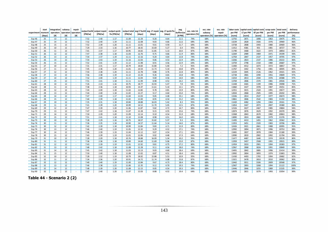
143


experiment

start

moment

[days]

integration

operators

[#]

subassy

operators

[#]

repair

operators

[#]

output build

[PM/w]

output repair

[PM/w]

output quick

fix [PM/w]

output total

[PM/w]

avg LT build

[days]

avg. LT repair

[days]

avg. LT quick fix

[days]

avg.

buffersize

[# PM]

occ. rate int

operators [%]

occ. rate

subassy

operators [%]

occ. rate

repair

operators [%]

labor costs

per PM

[euro]

capital costs

LT per PM

[euro]

capital costs

BT per PM

[euro]

scrap costs

per PM

[euro]

total costs

per PM

[euro]

delivery

performance

[%]

Exp 46 25 13 12 - 7.52 2.40 1.17 11.09 12.29 9.20 4.64 11.5 74% 68% - 12742 2871 1898 1963 19475 95%

Exp 47 25 14 12 - 7.52 2.40 1.19 11.11 12.08 9.03 4.66 11.6 69% 68% - 13239 2828 1926 1976 19969 96%

Exp 48 25 15 12 - 7.52 2.39 1.20 11.11 12.01 9.01 4.59 11.7 64% 68% - 13738 2808 1943 1980 20469 96%

Exp 49 26 10 12 - 7.29 2.33 1.16 10.77 18.42 15.69 5.27 6.4 95% 68% - 11412 4381 953 1981 18727 73%

Exp 50 26 11 12 - 7.41 2.37 1.17 10.95 14.65 11.85 5.13 10.0 87% 68% - 11790 3468 1622 1973 18854 81%

Exp 51 26 12 12 - 7.47 2.38 1.18 11.03 12.76 9.75 4.66 11.9 80% 68% - 12269 2989 1969 1971 19199 93%

Exp 52 26 13 12 - 7.54 2.37 1.19 11.11 12.16 9.20 4.64 12.8 74% 68% - 12764 2847 2137 1957 19705 97%

Exp 53 26 14 12 - 7.54 2.43 1.19 11.16 12.03 9.06 4.53 12.9 69% 69% - 13266 2823 2147 1986 20222 96%

Exp 54 26 15 12 - 7.52 2.41 1.19 11.12 11.98 8.91 4.56 12.9 64% 68% - 13759 2798 2150 1980 20687 97%

Exp 55 27 10 12 - 7.31 2.31 1.17 10.79 18.60 15.80 5.40 7.2 95% 68% - 11400 4412 1073 1972 18857 73%

Exp 56 27 11 12 - 7.45 2.36 1.20 11.01 14.54 11.73 5.10 10.8 87% 68% - 11767 3442 1756 1981 18945 85%

Exp 57 27 12 12 - 7.54 2.38 1.20 11.11 12.78 9.88 4.76 12.8 80% 68% - 12229 3005 2126 1962 19321 92%

Exp 58 27 13 12 - 7.56 2.38 1.19 11.12 12.24 9.26 4.65 13.8 74% 68% - 12738 2865 2290 1955 19849 97%

Exp 59 27 14 12 - 7.52 2.40 1.19 11.11 12.04 9.00 4.56 14.0 68% 68% - 13254 2813 2344 1976 20388 97%

Exp 60 27 15 12 - 7.51 2.41 1.18 11.11 11.99 8.98 4.52 14.2 64% 68% - 13769 2806 2370 1981 20926 98%

Exp 61 28 10 12 - 7.26 2.33 1.16 10.75 18.77 15.93 5.47 7.8 95% 68% - 11448 4465 1199 1986 19098 75%

Exp 62 28 11 12 - 7.38 2.36 1.18 10.93 14.47 11.61 5.10 12.1 87% 68% - 11860 3427 1978 1987 19251 85%

Exp 63 28 12 12 - 7.44 2.40 1.18 11.02 12.82 9.78 4.81 13.9 80% 69% - 12351 3015 2320 1991 19677 94%

Exp 64 28 13 12 - 7.44 2.40 1.18 11.02 12.27 9.17 4.60 15.0 74% 68% - 12834 2868 2505 1995 20202 98%

Exp 65 28 14 12 - 7.47 2.40 1.17 11.04 12.03 9.05 4.48 15.1 68% 69% - 13346 2814 2537 1977 20673 98%

Exp 66 28 15 12 - 7.44 2.39 1.18 11.02 12.00 8.95 4.54 15.2 64% 68% - 13861 2806 2542 1983 21192 98%

Exp 67 29 10 12 - 7.35 2.31 1.18 10.84 18.88 16.03 5.42 8.3 95% 68% - 11420 4482 1294 1964 19161 75%

Exp 68 29 11 12 - 7.41 2.39 1.20 10.99 14.52 11.70 5.05 12.5 87% 68% - 11854 3447 2073 2007 19380 86%

Exp 69 29 12 12 - 7.47 2.39 1.20 11.06 12.87 9.82 4.72 14.7 80% 68% - 12326 3027 2467 1985 19804 94%

Exp 70 29 13 12 - 7.47 2.42 1.18 11.07 12.28 9.15 4.55 15.6 74% 68% - 12874 2876 2629 1992 20370 98%

Exp 71 29 14 12 - 7.50 2.39 1.20 11.09 12.14 9.10 4.54 15.9 68% 68% - 13368 2843 2670 1982 20863 98%

Exp 72 29 15 12 - 7.51 2.41 1.18 11.10 12.08 8.98 4.51 16.0 64% 68% - 13890 2824 2682 1979 21376 98%

Exp 73 30 10 12 - 7.28 2.29 1.16 10.75 18.57 15.82 5.37 9.3 95% 68% - 11495 4413 1491 1962 19362 81%

Exp 74 30 11 12 - 7.36 2.35 1.18 10.90 14.57 11.64 5.14 14.0 87% 68% - 11953 3451 2320 1983 19706 88%

Exp 75 30 12 12 - 7.42 2.39 1.18 10.99 12.84 9.83 4.71 15.9 80% 68% - 12426 3021 2661 1988 20095 95%

Exp 76 30 13 12 - 7.46 2.40 1.19 11.05 12.32 9.29 4.52 17.1 74% 68% - 12992 2894 2871 1996 20753 98%

Exp 77 30 14 12 - 7.46 2.39 1.19 11.04 12.12 9.07 4.54 17.1 69% 68% - 13481 2837 2878 1984 21180 99%

Exp 78 30 15 12 - 7.43 2.39 1.19 11.01 12.06 9.02 4.48 17.3 64% 68% - 13990 2819 2902 1992 21704 99%

Exp 79 31 10 12 - 7.28 2.29 1.18 10.76 18.88 16.09 5.34 10.2 95% 68% - 11477 4487 1640 1974 19578 80%

Exp 80 31 11 12 - 7.36 2.36 1.18 10.89 14.60 11.69 5.06 15.0 87% 68% - 11959 3457 2508 1991 19915 89%

Exp 81 31 12 12 - 7.43 2.39 1.19 11.01 12.92 9.81 4.75 17.2 80% 68% - 12454 3033 2901 1994 20383 97%

Exp 82 31 13 12 - 7.48 2.42 1.18 11.08 12.28 9.11 4.56 18.0 74% 68% - 12967 2868 3024 1991 20849 99%

Exp 83 31 14 12 - 7.45 2.42 1.18 11.03 12.13 9.03 4.60 18.4 69% 68% - 13491 2842 3085 1996 21414 99%

Exp 84 31 15 12 - 7.50 2.40 1.18 11.08 12.02 8.87 4.51 18.4 64% 68% - 13992 2804 3093 1974 21863 99%

Exp 85 32 10 12 - 7.28 2.32 1.19 10.79 18.92 15.88 5.53 10.9 95% 68% - 11430 4493 1765 1994 19682 82%

Exp 86 32 11 12 - 7.34 2.36 1.20 10.91 14.72 11.74 5.08 15.8 87% 68% - 11921 3478 2653 2010 20062 90%

Exp 87 32 12 12 - 7.40 2.40 1.19 11.00 12.84 9.67 4.73 18.4 80% 68% - 12442 3011 3106 2009 20568 97%

Exp 88 32 13 12 - 7.46 2.38 1.22 11.06 12.35 9.12 4.70 19.3 74% 68% - 12967 2893 3268 1994 21122 100%

Exp 89 32 14 12 - 7.48 2.39 1.20 11.08 12.15 9.05 4.54 19.3 69% 68% - 13446 2846 3255 1989 21535 99%

Exp 90 32 15 12 - 7.47 2.40 1.20 11.07 12.03 8.88 4.52 19.4 64% 68% - 13970 2811 3279 1993 22054 99%

144


experiment

start

moment

[days]

integration

operators

[#]

subassy

operators

[#]

repair

operators

[#]

output build

[PM/w]

output repair

[PM/w]

output quick

fix [PM/w]

output total

[PM/w]

avg LT build

[days]

avg. LT repair

[days]

avg. LT quick fix

[days]

avg.

buffersize

[# PM]

occ. rate int

operators [%]

occ. rate

subassy

operators [%]

occ. rate

repair

operators [%]

labor costs

per PM

[euro]

capital costs

LT per PM

[euro]

capital costs

BT per PM

[euro]

scrap costs

per PM

[euro]

total costs

per PM

[euro]

delivery

performance

[%]

Exp 01 18 7 12 3 6.87 2.27 1.11 10.25 32.50 11.88 3.90 0.2 100% 69% 66% 12476 6691 22 2036 21225 14%

Exp 02 18 8 12 3 7.36 2.37 1.15 10.87 16.80 11.31 4.36 2.2 91% 69% 70% 12143 3818 284 1977 18222 43%

Exp 03 18 9 12 3 7.55 2.41 1.20 11.15 13.45 11.24 4.71 3.4 82% 70% 71% 12330 3214 477 1975 17996 64%

Exp 04 18 10 12 3 7.55 2.43 1.19 11.16 12.76 10.99 4.84 4.0 73% 70% 72% 12829 3084 579 1982 18473 69%

Exp 05 18 11 12 3 7.56 2.41 1.21 11.18 12.42 11.10 5.01 4.2 67% 70% 72% 13344 3029 610 1981 18965 71%

Exp 06 18 12 12 3 7.57 2.43 1.18 11.17 12.44 11.05 5.14 4.1 61% 70% 72% 13852 3035 601 1975 19463 74%

Exp 07 19 7 12 3 6.85 2.26 1.11 10.22 34.55 11.66 3.81 0.2 100% 69% 65% 12506 7045 36 2033 21619 16%

Exp 08 19 8 12 3 7.33 2.37 1.17 10.87 16.93 11.23 4.45 3.1 91% 70% 70% 12158 3842 432 1996 18428 47%

Exp 09 19 9 12 3 7.54 2.43 1.17 11.14 13.50 11.05 4.98 4.3 82% 70% 72% 12357 3223 635 1978 18193 68%

Exp 10 19 10 12 3 7.60 2.41 1.19 11.19 12.69 11.33 5.29 4.9 74% 70% 72% 12851 3103 738 1959 18651 74%

Exp 11 19 11 12 3 7.55 2.40 1.17 11.11 12.56 10.84 4.88 5.0 67% 70% 71% 13385 3034 759 1960 19138 79%

Exp 12 19 12 12 3 7.54 2.42 1.18 11.14 12.46 11.13 5.23 5.0 61% 70% 71% 13932 3052 753 1978 19715 76%

Exp 13 20 7 12 3 6.85 2.27 1.11 10.23 34.01 11.81 3.98 0.3 100% 69% 66% 12506 6965 37 2045 21553 16%

Exp 14 20 8 12 3 7.33 2.38 1.17 10.89 16.59 11.57 4.84 3.6 91% 70% 70% 12157 3814 504 2006 18481 53%

Exp 15 20 9 12 3 7.55 2.39 1.18 11.12 13.53 11.49 4.78 5.2 82% 70% 71% 12331 3242 789 1954 18317 73%

Exp 16 20 10 12 3 7.55 2.41 1.19 11.15 12.64 11.13 5.23 5.7 74% 70% 71% 12829 3073 883 1975 18760 80%

Exp 17 20 11 12 3 7.54 2.39 1.18 11.13 12.50 11.05 5.06 6.2 67% 70% 71% 13344 3036 957 1962 19298 83%

Exp 18 20 12 12 3 7.54 2.41 1.17 11.13 12.51 11.31 5.26 5.9 61% 70% 72% 13857 3067 904 1966 19794 79%

Exp 19 21 7 12 3 6.85 2.26 1.10 10.22 34.39 11.72 3.88 0.3 100% 69% 66% 12480 7023 44 2028 21575 18%

Exp 20 21 8 12 3 7.32 2.37 1.17 10.86 16.83 11.34 4.59 4.3 91% 70% 70% 12115 3831 650 2002 18597 55%

Exp 21 21 9 12 3 7.50 2.43 1.17 11.11 13.33 11.75 5.06 5.9 82% 70% 72% 12307 3236 908 1989 18440 77%

Exp 22 21 10 12 3 7.50 2.42 1.18 11.10 12.66 11.52 5.29 6.5 74% 70% 72% 12803 3113 1018 1983 18917 82%

Exp 23 21 11 12 3 7.50 2.42 1.19 11.11 12.52 11.19 5.46 6.6 67% 70% 72% 13294 3062 1042 1994 19393 85%

Exp 24 21 12 12 3 7.49 2.39 1.19 11.08 12.46 11.14 5.44 6.6 61% 70% 71% 13823 3043 1045 1980 19892 86%

Exp 25 22 7 12 3 6.88 2.25 1.13 10.27 33.48 12.15 4.07 0.5 100% 69% 66% 12469 6890 65 2035 21459 20%

Exp 26 22 8 12 3 7.27 2.36 1.18 10.81 16.78 11.53 4.71 5.0 91% 70% 70% 12165 3842 760 2012 18779 60%

Exp 27 22 9 12 3 7.54 2.42 1.18 11.13 13.44 11.43 5.28 6.9 82% 70% 72% 12310 3240 1089 1975 18615 79%

Exp 28 22 10 12 3 7.54 2.45 1.15 11.14 12.65 11.22 5.22 7.6 74% 70% 72% 12791 3083 1209 1976 19059 87%

Exp 29 22 11 12 3 7.56 2.39 1.19 11.14 12.45 11.34 5.09 7.5 67% 70% 71% 13308 3044 1197 1959 19508 87%

Exp 30 22 12 12 3 7.53 2.39 1.19 11.13 12.42 11.43 5.43 7.7 61% 70% 72% 13843 3060 1232 1968 20103 86%

Exp 31 23 7 12 3 6.88 2.25 1.11 10.24 33.83 11.88 3.89 0.4 100% 69% 66% 12482 6928 58 2024 21491 20%

Exp 32 23 8 12 3 7.31 2.42 1.17 10.89 16.59 12.03 4.69 5.6 91% 70% 71% 12146 3853 884 2034 18917 62%

Exp 33 23 9 12 3 7.58 2.45 1.17 11.20 13.42 11.72 5.12 8.0 82% 70% 72% 12317 3250 1272 1978 18816 84%

Exp 34 23 10 12 3 7.58 2.42 1.19 11.20 12.63 11.35 5.11 8.4 74% 70% 72% 12801 3078 1343 1969 19192 87%

Exp 35 23 11 12 3 7.55 2.41 1.19 11.15 12.51 11.11 5.32 8.6 67% 70% 71% 13318 3047 1393 1975 19733 89%

Exp 36 23 12 12 3 7.58 2.39 1.20 11.17 12.41 11.23 5.38 9.1 61% 70% 71% 13856 3045 1467 1963 20331 91%

Exp 37 24 7 12 3 6.84 2.25 1.11 10.21 34.86 11.68 3.75 0.5 100% 69% 65% 12506 7100 62 2035 21702 22%

Exp 38 24 8 12 3 7.31 2.40 1.20 10.92 16.75 11.97 5.03 6.4 91% 70% 71% 12118 3886 1022 2039 19064 65%

Exp 39 24 9 12 3 7.52 2.39 1.20 11.11 13.48 11.61 4.95 8.8 82% 70% 71% 12310 3243 1414 1977 18944 87%

Exp 40 24 10 12 3 7.53 2.41 1.19 11.14 12.62 11.47 5.28 9.7 74% 70% 71% 12819 3090 1576 1976 19461 90%

Exp 41 24 11 12 3 7.56 2.42 1.19 11.17 12.41 11.48 5.16 9.8 67% 70% 72% 13360 3049 1600 1978 19987 91%

Exp 42 24 12 12 3 7.54 2.40 1.19 11.12 12.43 11.61 5.03 9.7 61% 70% 71% 13853 3057 1573 1972 20454 92%

Exp 43 25 7 12 3 6.81 2.28 1.13 10.23 34.60 11.82 3.96 0.6 100% 69% 67% 12453 7077 79 2073 21683 24%

Exp 44 25 8 12 3 7.24 2.41 1.16 10.81 16.80 12.11 4.80 7.5 91% 70% 70% 12072 3897 1207 2042 19217 69%

Exp 45 25 9 12 3 7.51 2.45 1.17 11.12 13.52 11.58 5.04 9.8 82% 70% 71% 12268 3261 1604 1995 19128 91%

145


experiment

start

moment

[days]

integration

operators

[#]

subassy

operators

[#]

repair

operators

[#]

output build

[PM/w]

output repair

[PM/w]

output quick

fix [PM/w]

output total

[PM/w]

avg LT build

[days]

avg. LT repair

[days]

avg. LT quick fix

[days]

avg.

buffersize

[# PM]

occ. rate int

operators [%]

occ. rate

subassy

operators [%]

occ. rate

repair

operators [%]

labor costs

per PM

[euro]

capital costs

LT per PM

[euro]

capital costs

BT per PM

[euro]

scrap costs

per PM

[euro]

total costs

per PM

[euro]

delivery

performance

[%]

Exp 46 25 10 12 3 7.57 2.43 1.18 11.18 12.68 11.70 5.31 10.5 74% 70% 71% 12748 3119 1707 1974 19548 94%

Exp 47 25 11 12 3 7.56 2.40 1.18 11.15 12.49 11.55 5.34 10.8 67% 70% 71% 13234 3072 1761 1964 20031 93%

Exp 48 25 12 12 3 7.54 2.41 1.18 11.13 12.45 11.17 5.44 10.9 61% 70% 70% 13739 3039 1795 1967 20539 94%

Exp 49 26 7 12 3 6.84 2.27 1.14 10.25 33.30 12.01 4.00 0.8 100% 69% 67% 12431 6852 88 2058 21429 28%

Exp 50 26 8 12 3 7.29 2.37 1.21 10.88 16.45 12.17 5.37 8.3 91% 70% 71% 12037 3845 1369 2033 19284 72%

Exp 51 26 9 12 3 7.50 2.42 1.17 11.10 13.35 11.50 5.43 11.1 82% 70% 71% 12287 3231 1822 1980 19321 91%

Exp 52 26 10 12 3 7.52 2.44 1.16 11.13 12.65 11.52 5.36 11.5 74% 70% 71% 12753 3107 1899 1977 19735 95%

Exp 53 26 11 12 3 7.56 2.41 1.16 11.13 12.47 11.28 5.40 12.0 67% 70% 71% 13272 3052 1977 1954 20254 95%

Exp 54 26 12 12 3 7.58 2.46 1.16 11.20 12.41 11.83 5.62 11.8 61% 70% 72% 13784 3095 1931 1981 20791 94%

Exp 55 27 7 12 3 6.79 2.26 1.13 10.18 33.69 11.73 3.81 1.0 100% 69% 66% 12438 6892 112 2063 21505 31%

Exp 56 27 8 12 3 7.34 2.40 1.18 10.91 16.50 12.32 4.92 9.1 91% 70% 70% 12021 3847 1504 2016 19387 76%

Exp 57 27 9 12 3 7.54 2.39 1.19 11.12 13.42 11.74 5.30 12.3 82% 70% 71% 12270 3245 2022 1964 19501 95%

Exp 58 27 10 12 3 7.52 2.42 1.17 11.11 12.67 11.64 5.59 12.7 74% 70% 71% 12772 3122 2113 1978 19986 96%

Exp 59 27 11 12 3 7.60 2.43 1.18 11.20 12.54 11.46 5.30 12.9 67% 70% 71% 13275 3081 2123 1966 20444 96%

Exp 60 27 12 12 3 7.54 2.42 1.18 11.13 12.45 11.36 5.10 12.9 61% 70% 71% 13773 3055 2125 1975 20929 95%

Exp 61 28 7 12 3 6.85 2.29 1.11 10.25 34.09 11.96 3.97 1.1 100% 69% 66% 12438 6990 129 2056 21612 30%

Exp 62 28 8 12 3 7.33 2.38 1.18 10.90 16.58 12.24 4.95 10.2 91% 70% 70% 12064 3860 1709 2010 19643 76%

Exp 63 28 9 12 3 7.52 2.43 1.19 11.13 13.30 12.07 5.29 12.9 82% 70% 72% 12333 3256 2136 1990 19714 95%

Exp 64 28 10 12 3 7.53 2.39 1.19 11.10 12.61 11.37 5.18 13.9 74% 70% 70% 12823 3077 2301 1968 20169 97%

Exp 65 28 11 12 3 7.58 2.45 1.19 11.21 12.45 11.39 5.32 14.2 67% 70% 72% 13364 3062 2358 1986 20769 97%

Exp 66 28 12 12 3 7.55 2.42 1.19 11.16 12.36 11.32 5.57 14.4 61% 70% 71% 13906 3048 2388 1980 21322 97%

Exp 67 29 7 12 3 6.82 2.28 1.15 10.25 33.69 11.96 4.00 1.3 100% 69% 67% 12433 6923 138 2080 21574 33%

Exp 68 29 8 12 3 7.34 2.41 1.19 10.94 16.74 12.51 5.05 10.6 91% 70% 71% 12043 3917 1777 2031 19767 77%

Exp 69 29 9 12 3 7.58 2.43 1.17 11.17 13.34 12.26 5.76 13.9 82% 70% 72% 12375 3292 2312 1967 19946 95%

Exp 70 29 10 12 3 7.58 2.42 1.19 11.18 12.70 11.35 5.38 14.7 74% 70% 71% 12815 3102 2441 1971 20329 97%

Exp 71 29 11 12 3 7.59 2.41 1.20 11.20 12.42 11.55 5.32 14.8 67% 70% 72% 13343 3064 2462 1964 20834 98%

Exp 72 29 12 12 3 7.56 2.41 1.19 11.16 12.38 11.31 5.15 15.2 61% 70% 71% 13874 3035 2530 1977 21415 98%

Exp 73 30 7 12 3 6.85 2.28 1.16 10.29 33.86 12.08 3.95 1.4 100% 69% 67% 12393 6955 151 2080 21579 37%

Exp 74 30 8 12 3 7.33 2.41 1.16 10.90 16.54 12.57 5.16 12.0 91% 70% 71% 12097 3887 2024 2016 20023 80%

Exp 75 30 9 12 3 7.58 2.40 1.19 11.17 13.35 11.73 5.11 15.3 82% 70% 71% 12460 3239 2547 1957 20203 95%

Exp 76 30 10 12 3 7.58 2.37 1.17 11.12 12.64 11.44 5.25 16.1 73% 70% 71% 12944 3088 2688 1934 20655 98%

Exp 77 30 11 12 3 7.56 2.36 1.19 11.12 12.45 11.24 5.40 16.5 67% 70% 71% 13462 3048 2749 1947 21205 99%

Exp 78 30 12 12 3 7.59 2.38 1.20 11.17 12.38 11.16 5.48 16.3 61% 70% 71% 13962 3037 2718 1958 21675 99%

Exp 79 31 7 12 3 6.82 2.29 1.12 10.24 33.68 12.03 3.84 1.8 100% 69% 67% 12430 6918 202 2066 21615 43%

Exp 80 31 8 12 3 7.34 2.39 1.17 10.91 16.82 12.24 5.07 12.8 91% 70% 70% 12118 3917 2168 2010 20213 80%

Exp 81 31 9 12 3 7.54 2.42 1.17 11.13 13.41 12.13 5.30 15.9 82% 70% 71% 12430 3281 2651 1969 20331 95%

Exp 82 31 10 12 3 7.56 2.40 1.18 11.14 12.76 11.50 5.60 17.2 74% 70% 71% 12944 3124 2867 1959 20894 99%

Exp 83 31 11 12 3 7.59 2.39 1.19 11.17 12.50 11.75 5.62 17.2 67% 70% 71% 13458 3099 2873 1952 21382 98%

Exp 84 31 12 12 3 7.59 2.39 1.18 11.17 12.45 11.64 5.40 17.2 61% 70% 71% 13976 3073 2876 1950 21874 98%

Exp 85 32 7 12 3 6.78 2.28 1.13 10.20 34.27 12.08 3.90 1.9 100% 69% 67% 12418 7036 226 2081 21760 44%

Exp 86 32 8 12 3 7.25 2.42 1.19 10.86 16.77 12.40 5.30 13.6 91% 70% 71% 12069 3927 2312 2064 20372 83%

Exp 87 32 9 12 3 7.45 2.37 1.19 11.01 13.49 11.89 5.08 17.4 82% 70% 71% 12453 3268 2914 1976 20611 96%

Exp 88 32 10 12 3 7.55 2.36 1.17 11.09 12.65 11.48 5.25 18.3 73% 70% 71% 12911 3088 3056 1941 20996 99%

Exp 89 32 11 12 3 7.53 2.38 1.20 11.10 12.51 11.58 5.33 18.3 67% 70% 71% 13448 3074 3059 1967 21549 99%

Exp 90 32 12 12 3 7.56 2.41 1.17 11.15 12.52 11.51 5.66 18.3 61% 70% 71% 13977 3095 3060 1963 22095 99%

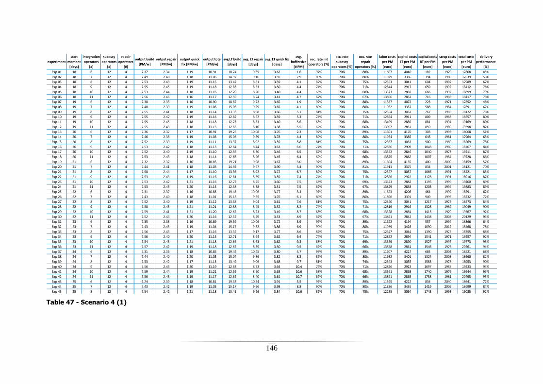
146


experiment

start

moment

[days]

integration

operators

[#]

subassy

operators

[#]

repair

operators

[#]

output build

[PM/w]

output repair

[PM/w]

output quick

fix [PM/w]

output total

[PM/w]

avg LT build

[days]

avg. LT repair

[days]

avg. LT quick fix

[days]

avg.

buffersize

[# PM]

occ. rate int

operators [%]

occ. rate

subassy

operators [%]

occ. rate

repair

operators [%]

labor costs

per PM

[euro]

capital costs

LT per PM

[euro]

capital costs

BT per PM

[euro]

scrap costs

per PM

[euro]

total costs

per PM

[euro]

delivery

performance

[%]

Exp 01 18 6 12 4 7.37 2.34 1.19 10.91 18.74 9.65 3.62 1.6 97% 70% 88% 11607 4040 182 1979 17808 45%

Exp 02 18 7 12 4 7.49 2.40 1.18 11.06 14.97 9.16 3.59 2.9 89% 70% 80% 11929 3336 394 1980 17639 56%

Exp 03 18 8 12 4 7.53 2.43 1.19 11.15 13.42 8.81 3.59 4.1 82% 70% 75% 12353 3041 604 1992 17989 67%

Exp 04 18 9 12 4 7.55 2.45 1.19 11.18 12.83 8.53 3.50 4.4 74% 70% 71% 12844 2917 659 1992 18412 76%

Exp 05 18 10 12 4 7.53 2.44 1.18 11.16 12.70 8.20 3.40 4.4 68% 70% 68% 13373 2869 666 1992 18899 79%

Exp 06 18 11 12 4 7.56 2.46 1.16 11.17 12.59 8.24 3.41 4.7 62% 70% 67% 13866 2852 716 1983 19417 78%

Exp 07 19 6 12 4 7.38 2.35 1.16 10.90 18.87 9.72 3.65 1.9 97% 70% 88% 11587 4072 223 1971 17852 48%

Exp 08 19 7 12 4 7.48 2.39 1.19 11.06 15.03 9.29 3.65 4.1 89% 70% 80% 11962 3357 588 1984 17891 62%

Exp 09 19 8 12 4 7.55 2.41 1.18 11.14 13.33 8.98 3.66 5.1 81% 70% 75% 12354 3032 767 1969 18122 76%

Exp 10 19 9 12 4 7.55 2.42 1.19 11.16 12.82 8.52 3.59 5.3 74% 70% 71% 12854 2911 809 1983 18557 80%

Exp 11 19 10 12 4 7.55 2.45 1.18 11.18 12.73 8.33 3.40 5.6 68% 70% 68% 13409 2885 881 1994 19169 80%

Exp 12 19 11 12 4 7.55 2.43 1.18 11.15 12.65 8.10 3.38 5.5 62% 70% 66% 13907 2851 859 1980 19598 82%

Exp 13 20 6 12 4 7.36 2.37 1.17 10.91 19.25 10.08 3.76 2.3 97% 70% 89% 11601 4170 303 1993 18068 51%

Exp 14 20 7 12 4 7.46 2.38 1.19 11.03 15.06 9.59 3.78 4.4 89% 70% 80% 11954 3385 645 1981 17964 65%

Exp 15 20 8 12 4 7.52 2.39 1.19 11.11 13.37 8.92 3.59 5.8 81% 70% 75% 12367 3033 900 1969 18269 78%

Exp 16 20 9 12 4 7.53 2.42 1.18 11.13 12.84 8.44 3.63 6.6 74% 70% 71% 12836 2909 1043 1980 18767 84%

Exp 17 20 10 12 4 7.52 2.40 1.19 11.10 12.56 8.30 3.46 6.5 67% 70% 68% 13352 2846 1040 1973 19211 87%

Exp 18 20 11 12 4 7.53 2.43 1.18 11.14 12.66 8.26 3.45 6.4 62% 70% 66% 13875 2862 1007 1984 19728 86%

Exp 19 21 6 12 4 7.32 2.37 1.16 10.85 19.21 9.98 3.67 3.0 97% 70% 89% 11604 4155 400 2000 18159 57%

Exp 20 21 7 12 4 7.44 2.41 1.18 11.03 14.94 9.67 3.90 5.4 90% 70% 81% 11911 3375 834 2001 18121 70%

Exp 21 21 8 12 4 7.50 2.44 1.17 11.10 13.36 8.92 3.72 6.7 82% 70% 75% 12327 3037 1066 1991 18421 83%

Exp 22 21 9 12 4 7.53 2.43 1.19 11.16 12.81 8.69 3.59 7.4 74% 70% 71% 12826 2922 1178 1991 18916 87%

Exp 23 21 10 12 4 7.53 2.42 1.21 11.16 12.72 8.25 3.60 7.5 68% 70% 69% 13323 2882 1195 1999 19400 89%

Exp 24 21 11 12 4 7.53 2.43 1.20 11.15 12.58 8.38 3.51 7.5 62% 70% 67% 13829 2858 1203 1994 19883 89%

Exp 25 22 6 12 4 7.31 2.37 1.16 10.85 19.45 10.06 3.77 3.3 97% 70% 89% 11623 4206 464 1999 18291 62%

Exp 26 22 7 12 4 7.43 2.40 1.18 11.01 15.13 9.55 3.76 6.1 89% 70% 80% 11896 3391 949 1996 18232 72%

Exp 27 22 8 12 4 7.52 2.40 1.19 11.12 13.38 9.04 3.61 7.6 81% 70% 75% 12340 3041 1217 1975 18573 84%

Exp 28 22 9 12 4 7.58 2.43 1.21 11.21 12.88 8.45 3.52 8.2 74% 70% 71% 12816 2916 1328 1989 19049 90%

Exp 29 22 10 12 4 7.59 2.41 1.21 11.20 12.62 8.23 3.49 8.7 68% 70% 68% 13328 2854 1415 1970 19567 92%

Exp 30 22 11 12 4 7.52 2.44 1.20 11.16 12.52 8.29 3.53 8.9 62% 70% 67% 13841 2842 1438 2008 20129 93%

Exp 31 23 6 12 4 7.35 2.38 1.16 10.89 19.39 10.06 3.72 3.9 97% 70% 89% 11622 4194 557 1994 18366 64%

Exp 32 23 7 12 4 7.43 2.43 1.19 11.04 15.17 9.82 3.86 6.9 90% 70% 80% 11939 3426 1090 2012 18468 78%

Exp 33 23 8 12 4 7.56 2.43 1.17 11.16 13.32 9.17 3.77 8.6 82% 70% 75% 12347 3044 1390 1975 18755 88%

Exp 34 23 9 12 4 7.56 2.40 1.20 11.15 12.71 8.64 3.62 9.4 74% 70% 71% 12852 2894 1541 1971 19257 92%

Exp 35 23 10 12 4 7.54 2.43 1.21 11.18 12.66 8.63 3.62 9.3 68% 70% 69% 13359 2890 1527 1997 19773 93%

Exp 36 23 11 12 4 7.57 2.42 1.19 11.18 12.62 8.39 3.50 9.5 62% 70% 66% 13878 2861 1546 1976 20261 94%

Exp 37 24 6 12 4 7.31 2.36 1.18 10.85 19.44 10.45 3.80 4.7 97% 70% 89% 11607 4227 684 2003 18521 68%

Exp 38 24 7 12 4 7.44 2.40 1.20 11.05 15.04 9.86 3.82 8.3 89% 70% 80% 11932 3401 1324 2003 18660 82%

Exp 39 24 8 12 4 7.53 2.42 1.17 11.13 13.49 9.06 3.68 9.7 81% 70% 74% 12343 3055 1583 1973 18953 90%

Exp 40 24 9 12 4 7.56 2.43 1.20 11.19 12.83 8.73 3.64 10.4 74% 70% 71% 12826 2923 1697 1987 19433 94%

Exp 41 24 10 12 4 7.59 2.44 1.19 11.21 12.59 8.50 3.63 10.6 68% 70% 68% 13361 2868 1740 1976 19944 95%

Exp 42 24 11 12 4 7.56 2.43 1.19 11.17 12.62 8.40 3.61 10.7 62% 70% 66% 13891 2865 1758 1981 20495 95%

Exp 43 25 6 12 4 7.24 2.39 1.18 10.81 19.33 10.54 3.91 5.5 97% 70% 89% 11545 4222 834 2040 18641 72%

Exp 44 25 7 12 4 7.43 2.42 1.19 11.03 15.17 9.96 3.98 8.8 90% 70% 80% 11836 3435 1419 2009 18699 84%

Exp 45 25 8 12 4 7.54 2.42 1.21 11.18 13.41 9.26 3.84 10.6 82% 70% 75% 12235 3064 1743 1993 19035 92%

147


experiment

start

moment

[days]

integration

operators

[#]

subassy

operators

[#]

repair

operators

[#]

output build

[PM/w]

output repair

[PM/w]

output quick

fix [PM/w]

output total

[PM/w]

avg LT build

[days]

avg. LT repair

[days]

avg. LT quick fix

[days]

avg.

buffersize

[# PM]

occ. rate int

operators [%]

occ. rate

subassy

operators [%]

occ. rate

repair

operators [%]

labor costs

per PM

[euro]

capital costs

LT per PM

[euro]

capital costs

BT per PM

[euro]

scrap costs

per PM

[euro]

total costs

per PM

[euro]

delivery

performance

[%]

Exp 46 25 9 12 4 7.52 2.43 1.18 11.13 12.89 8.66 3.64 11.2 74% 70% 71% 12743 2934 1844 1991 19511 94%

Exp 47 25 10 12 4 7.50 2.41 1.19 11.09 12.70 8.40 3.54 11.5 68% 70% 68% 13243 2873 1893 1986 19995 96%

Exp 48 25 11 12 4 7.54 2.39 1.20 11.13 12.66 8.29 3.52 11.9 62% 70% 66% 13769 2856 1976 1968 20570 97%

Exp 49 26 6 12 4 7.28 2.41 1.19 10.88 19.76 10.41 3.97 6.1 97% 70% 89% 11566 4301 930 2047 18844 73%

Exp 50 26 7 12 4 7.40 2.43 1.17 11.00 15.27 9.72 3.81 9.7 89% 70% 80% 11879 3431 1581 2013 18904 84%

Exp 51 26 8 12 4 7.50 2.45 1.19 11.14 13.46 9.17 3.70 11.5 82% 70% 75% 12287 3072 1896 2010 19264 92%

Exp 52 26 9 12 4 7.59 2.43 1.18 11.20 12.83 8.53 3.56 12.5 74% 70% 71% 12764 2908 2077 1971 19720 97%

Exp 53 26 10 12 4 7.56 2.41 1.18 11.16 12.66 8.49 3.50 12.6 68% 70% 68% 13286 2871 2090 1965 20212 97%

Exp 54 26 11 12 4 7.56 2.43 1.21 11.20 12.63 8.52 3.58 12.6 62% 70% 67% 13794 2873 2099 1988 20753 97%

Exp 55 27 6 12 4 7.26 2.39 1.18 10.83 19.62 10.69 3.96 7.0 97% 70% 89% 11580 4290 1106 2032 19008 79%

Exp 56 27 7 12 4 7.42 2.43 1.19 11.03 15.30 9.90 3.92 10.9 89% 70% 80% 11870 3447 1797 2014 19127 85%

Exp 57 27 8 12 4 7.56 2.42 1.21 11.19 13.51 9.23 3.83 12.6 81% 70% 75% 12254 3080 2091 1988 19413 94%

Exp 58 27 9 12 4 7.58 2.46 1.18 11.21 12.96 8.65 3.72 13.2 74% 70% 71% 12752 2950 2189 1985 19875 96%

Exp 59 27 10 12 4 7.58 2.44 1.19 11.21 12.61 8.62 3.47 13.8 68% 70% 68% 13264 2868 2299 1981 20413 98%

Exp 60 27 11 12 4 7.58 2.44 1.21 11.23 12.58 8.49 3.63 13.8 62% 70% 66% 13776 2867 2287 1990 20920 98%

Exp 61 28 6 12 4 7.28 2.41 1.19 10.87 19.80 10.76 3.95 7.5 97% 70% 89% 11553 4323 1189 2045 19110 78%

Exp 62 28 7 12 4 7.47 2.41 1.20 11.07 15.16 9.91 3.78 12.2 89% 70% 80% 11928 3421 2014 1998 19362 91%

Exp 63 28 8 12 4 7.59 2.44 1.18 11.21 13.47 9.15 3.81 13.8 81% 70% 74% 12355 3070 2298 1975 19697 95%

Exp 64 28 9 12 4 7.55 2.45 1.20 11.19 12.83 8.66 3.70 14.7 74% 70% 71% 12834 2922 2448 1999 20203 98%

Exp 65 28 10 12 4 7.56 2.45 1.18 11.19 12.68 8.68 3.67 14.6 68% 70% 68% 13363 2895 2443 1988 20690 98%

Exp 66 28 11 12 4 7.63 2.44 1.17 11.24 12.59 8.51 3.59 15.0 62% 70% 66% 13886 2863 2506 1962 21217 98%

Exp 67 29 6 12 4 7.28 2.37 1.18 10.83 19.88 10.64 4.12 8.4 97% 69% 89% 11551 4327 1362 2016 19256 84%

Exp 68 29 7 12 4 7.46 2.44 1.19 11.09 15.20 10.06 3.98 12.9 90% 70% 80% 11920 3456 2155 2013 19543 89%

Exp 69 29 8 12 4 7.58 2.42 1.19 11.18 13.49 9.20 3.72 14.8 81% 70% 75% 12340 3075 2457 1970 19842 95%

Exp 70 29 9 12 4 7.56 2.44 1.19 11.20 12.86 8.87 3.62 15.7 74% 70% 71% 12877 2940 2619 1987 20423 98%

Exp 71 29 10 12 4 7.59 2.43 1.18 11.20 12.55 8.70 3.55 15.9 68% 70% 68% 13368 2871 2656 1974 20868 98%

Exp 72 29 11 12 4 7.58 2.46 1.18 11.22 12.65 8.42 3.63 15.7 62% 70% 66% 13873 2874 2622 1989 21358 98%

Exp 73 30 6 12 4 7.27 2.41 1.15 10.84 19.43 10.60 4.00 9.5 97% 70% 89% 11636 4254 1572 2028 19491 86%

Exp 74 30 7 12 4 7.46 2.39 1.19 11.05 15.09 10.16 3.95 14.0 89% 70% 80% 12002 3434 2337 1985 19758 90%

Exp 75 30 8 12 4 7.55 2.45 1.19 11.19 13.50 9.36 3.83 16.0 82% 70% 75% 12452 3092 2669 1996 20210 96%

Exp 76 30 9 12 4 7.58 2.40 1.20 11.18 12.91 8.74 3.68 16.6 74% 70% 71% 12966 2938 2775 1968 20647 99%

Exp 77 30 10 12 4 7.55 2.41 1.21 11.18 12.68 8.58 3.56 17.1 68% 70% 68% 13472 2885 2865 1986 21207 99%

Exp 78 30 11 12 4 7.55 2.40 1.19 11.14 12.60 8.41 3.45 17.1 62% 70% 66% 13994 2857 2859 1970 21679 99%

Exp 79 31 6 12 4 7.29 2.41 1.16 10.86 19.84 11.03 4.17 10.0 97% 70% 89% 11617 4357 1646 2026 19646 85%

Exp 80 31 7 12 4 7.43 2.40 1.17 10.98 15.28 9.94 4.00 15.1 89% 70% 80% 12021 3453 2545 1988 20006 92%

Exp 81 31 8 12 4 7.53 2.42 1.20 11.14 13.40 9.29 3.89 17.0 81% 70% 75% 12445 3071 2855 1987 20358 97%

Exp 82 31 9 12 4 7.53 2.41 1.19 11.12 12.90 8.99 3.68 17.5 74% 70% 71% 12929 2954 2930 1977 20790 98%

Exp 83 31 10 12 4 7.58 2.40 1.21 11.18 12.65 8.60 3.54 18.2 68% 70% 68% 13486 2879 3059 1966 21389 99%

Exp 84 31 11 12 4 7.55 2.41 1.17 11.12 12.56 8.61 3.54 18.3 62% 70% 66% 14012 2865 3072 1960 21908 99%

Exp 85 32 6 12 4 7.23 2.40 1.19 10.83 19.88 11.06 4.09 10.9 97% 70% 89% 11589 4371 1817 2056 19833 88%

Exp 86 32 7 12 4 7.37 2.41 1.20 10.97 15.17 10.28 4.10 15.8 89% 70% 80% 11979 3465 2662 2024 20129 93%

Exp 87 32 8 12 4 7.48 2.43 1.21 11.11 13.65 9.50 3.93 17.7 82% 70% 75% 12417 3132 2962 2014 20525 97%

Exp 88 32 9 12 4 7.52 2.40 1.19 11.11 12.87 8.88 3.73 18.9 74% 70% 71% 12930 2942 3163 1974 21009 99%

Exp 89 32 10 12 4 7.53 2.39 1.18 11.11 12.72 8.60 3.52 19.2 68% 70% 68% 13449 2895 3221 1961 21527 99%

Exp 90 32 11 12 4 7.55 2.40 1.18 11.13 12.65 8.49 3.55 19.2 62% 70% 66% 13960 2870 3209 1961 22000 99%

148

Table 49 - Scenario 1, yield 88% (1)

experiment

start

moment

[days]

integration

operators

[#]

subassy

operators

[#]

repair

operators

[#]

output build

[PM/w]

output repair

[PM/w]

output quick

fix [PM/w]

output total

[PM/w]

avg LT build

[days]

avg. LT repair

[days]

avg. LT quick fix

[days]

avg.

buffersize

[# PM]

occ. rate int

operators [%]

occ. rate

subassy

operators [%]

occ. rate

repair

operators [%]

labor costs

per PM

[euro]

capital costs

LT per PM

[euro]

capital costs

BT per PM

[euro]

scrap costs

per PM

[euro]

total costs

per PM

[euro]

delivery

performance

[%]

Exp 01 18 8 12 - 7.20 0.72 0.35 8.27 20.68 17.87 7.90 2.5 94% 65% - 10199 3993 379 615 15186 55%

Exp 02 18 9 12 - 7.29 0.74 0.35 8.38 14.21 11.62 6.33 4.8 84% 66% - 10591 2777 804 619 14791 76%

Exp 03 18 10 12 - 7.32 0.75 0.34 8.41 12.09 9.25 5.66 6.0 76% 66% - 11104 2371 1038 616 15130 90%

Exp 04 18 11 12 - 7.33 0.76 0.34 8.43 11.57 8.83 5.38 6.3 69% 66% - 11622 2276 1086 622 15607 94%

Exp 05 18 12 12 - 7.35 0.76 0.33 8.44 11.43 8.84 5.32 6.6 63% 66% - 12166 2250 1136 616 16167 94%

Exp 06 18 13 12 - 7.33 0.76 0.34 8.43 11.33 8.81 5.21 6.6 58% 66% - 12678 2233 1130 620 16662 95%

Exp 07 19 8 12 - 7.21 0.74 0.33 8.27 20.15 17.08 7.81 3.1 94% 65% - 10189 3894 483 615 15181 64%

Exp 08 19 9 12 - 7.31 0.75 0.33 8.40 13.93 11.21 6.15 5.7 84% 66% - 10598 2722 974 615 14908 83%

Exp 09 19 10 12 - 7.34 0.74 0.34 8.42 12.13 9.45 5.57 6.8 76% 65% - 11107 2377 1179 611 15274 91%

Exp 10 19 11 12 - 7.32 0.75 0.34 8.41 11.54 8.92 5.35 7.3 69% 65% - 11641 2270 1262 615 15788 95%

Exp 11 19 12 12 - 7.31 0.75 0.34 8.40 11.38 8.88 5.25 7.6 63% 66% - 12173 2241 1310 616 16340 96%

Exp 12 19 13 12 - 7.32 0.75 0.34 8.41 11.35 8.84 5.25 7.6 58% 66% - 12693 2235 1303 619 16851 96%

Exp 13 20 8 12 - 7.21 0.72 0.34 8.26 20.29 17.30 8.05 3.7 94% 65% - 10202 3917 595 608 15322 67%

Exp 14 20 9 12 - 7.29 0.75 0.33 8.38 14.11 11.47 6.19 6.5 84% 66% - 10604 2752 1109 614 15078 84%

Exp 15 20 10 12 - 7.33 0.76 0.34 8.44 12.28 9.44 5.69 7.7 76% 65% - 11127 2408 1324 622 15480 93%

Exp 16 20 11 12 - 7.33 0.76 0.33 8.42 11.65 8.99 5.40 8.2 69% 66% - 11649 2291 1408 619 15966 96%

Exp 17 20 12 12 - 7.34 0.75 0.34 8.44 11.45 8.61 5.39 8.3 63% 66% - 12170 2251 1440 616 16477 97%

Exp 18 20 13 12 - 7.34 0.76 0.34 8.44 11.41 8.48 5.39 8.3 58% 66% - 12695 2243 1438 620 16995 98%

Exp 19 21 8 12 - 7.23 0.73 0.34 8.30 20.22 17.04 7.70 4.4 94% 65% - 10182 3893 708 610 15393 71%

Exp 20 21 9 12 - 7.29 0.76 0.34 8.40 14.10 11.48 6.30 7.4 84% 66% - 10609 2759 1265 624 15257 86%

Exp 21 21 10 12 - 7.32 0.75 0.34 8.41 12.13 9.58 5.64 8.8 76% 65% - 11104 2378 1529 616 15627 96%

Exp 22 21 11 12 - 7.31 0.75 0.34 8.40 11.61 9.07 5.29 9.4 69% 66% - 11647 2283 1631 616 16178 97%

Exp 23 21 12 12 - 7.34 0.76 0.34 8.44 11.44 8.81 5.34 9.5 63% 66% - 12162 2249 1645 618 16673 98%

Exp 24 21 13 12 - 7.34 0.76 0.34 8.45 11.41 8.74 5.29 9.5 58% 66% - 12691 2242 1645 622 17199 99%

Exp 25 22 8 12 - 7.24 0.72 0.34 8.30 20.39 17.41 8.03 5.0 94% 65% - 10216 3928 827 606 15577 73%

Exp 26 22 9 12 - 7.29 0.75 0.35 8.39 14.14 11.35 6.27 8.2 84% 65% - 10606 2755 1413 621 15396 89%

Exp 27 22 10 12 - 7.34 0.75 0.35 8.44 12.18 9.67 5.62 9.8 76% 66% - 11112 2391 1697 619 15818 97%

Exp 28 22 11 12 - 7.36 0.75 0.35 8.46 11.61 9.07 5.43 10.4 69% 66% - 11643 2283 1797 618 16341 98%

Exp 29 22 12 12 - 7.37 0.75 0.34 8.47 11.43 8.80 5.33 10.7 63% 66% - 12177 2247 1840 614 16878 99%

Exp 30 22 13 12 - 7.35 0.76 0.34 8.45 11.41 8.72 5.22 10.6 58% 66% - 12710 2242 1835 616 17403 99%

Exp 31 23 8 12 - 7.23 0.71 0.34 8.28 20.18 17.04 8.06 5.7 94% 65% - 10175 3887 937 601 15600 74%

Exp 32 23 9 12 - 7.28 0.74 0.34 8.36 14.10 11.58 6.32 9.3 84% 66% - 10599 2753 1614 618 15584 90%

Exp 33 23 10 12 - 7.29 0.75 0.34 8.38 12.15 9.65 5.70 10.8 76% 65% - 11125 2389 1869 619 16002 97%

Exp 34 23 11 12 - 7.30 0.74 0.34 8.39 11.60 8.95 5.50 11.4 69% 65% - 11646 2276 1977 616 16514 99%

Exp 35 23 12 12 - 7.30 0.75 0.34 8.39 11.40 8.89 5.34 11.7 63% 65% - 12191 2243 2023 616 17073 99%

Exp 36 23 13 12 - 7.31 0.75 0.35 8.40 11.35 8.86 5.23 11.7 58% 65% - 12716 2234 2026 620 17596 99%

Exp 37 24 8 12 - 7.22 0.72 0.35 8.29 20.48 17.78 8.05 6.2 94% 65% - 10196 3952 1037 612 15797 76%

Exp 38 24 9 12 - 7.31 0.74 0.34 8.39 14.02 11.27 6.44 10.1 84% 65% - 10596 2734 1748 612 15690 92%

Exp 39 24 10 12 - 7.28 0.75 0.35 8.37 12.16 9.80 5.70 11.7 76% 65% - 11120 2389 2029 624 16162 97%

Exp 40 24 11 12 - 7.32 0.76 0.34 8.42 11.55 9.02 5.44 12.3 69% 66% - 11648 2271 2135 623 16676 99%

Exp 41 24 12 12 - 7.31 0.75 0.35 8.41 11.37 8.82 5.30 12.5 63% 65% - 12177 2235 2169 620 17201 99%

Exp 42 24 13 12 - 7.31 0.75 0.35 8.41 11.31 8.81 5.32 12.6 58% 65% - 12713 2227 2187 624 17750 99%

Exp 43 25 8 12 - 7.23 0.73 0.34 8.30 20.39 17.55 8.04 7.3 94% 65% - 10195 3932 1235 612 15975 79%

Exp 44 25 9 12 - 7.29 0.74 0.35 8.38 14.02 11.48 6.35 11.2 84% 66% - 10607 2740 1938 620 15905 93%

Exp 45 25 10 12 - 7.32 0.75 0.35 8.42 12.17 9.46 5.72 12.9 76% 66% - 11125 2384 2238 624 16372 99%

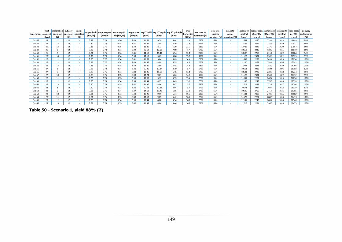
149

Table 50 - Scenario 1, yield 88% (2)

experiment

start

moment

[days]

integration

operators

[#]

subassy

operators

[#]

repair

operators

[#]

output build

[PM/w]

output repair

[PM/w]

output quick

fix [PM/w]

output total

[PM/w]

avg LT build

[days]

avg. LT repair

[days]

avg. LT quick fix

[days]

avg.

buffersize

[# PM]

occ. rate int

operators [%]

occ. rate

subassy

operators [%]

occ. rate

repair

operators [%]

labor costs

per PM

[euro]

capital costs

LT per PM

[euro]

capital costs

BT per PM

[euro]

scrap costs

per PM

[euro]

total costs

per PM

[euro]

delivery

performance

[%]

Exp 46 25 11 12 - 7.33 0.74 0.36 8.43 11.65 9.20 5.44 13.4 69% 65% - 11657 2290 2324 618 16889 99%

Exp 47 25 12 12 - 7.32 0.74 0.35 8.41 11.46 8.85 5.36 13.6 63% 65% - 12186 2252 2355 619 17411 99%

Exp 48 25 13 12 - 7.33 0.75 0.35 8.43 11.40 8.71 5.39 13.7 58% 65% - 12725 2242 2371 620 17957 99%

Exp 49 26 8 12 - 7.23 0.73 0.34 8.29 20.52 17.55 7.90 7.7 94% 65% - 10158 3945 1306 611 16019 80%

Exp 50 26 9 12 - 7.31 0.76 0.34 8.41 14.13 11.44 6.54 12.1 84% 65% - 10597 2756 2110 622 16084 94%

Exp 51 26 10 12 - 7.29 0.76 0.34 8.38 12.18 9.69 5.80 13.8 76% 65% - 11120 2392 2392 622 16525 99%

Exp 52 26 11 12 - 7.30 0.77 0.34 8.41 11.63 9.04 5.69 14.4 69% 66% - 11649 2283 2493 629 17054 100%

Exp 53 26 12 12 - 7.32 0.77 0.34 8.43 11.45 8.88 5.35 14.6 63% 66% - 12180 2252 2524 626 17582 100%

Exp 54 26 13 12 - 7.33 0.77 0.35 8.44 11.40 8.90 5.45 14.6 58% 66% - 12704 2243 2531 629 18107 100%

Exp 55 27 8 12 - 7.23 0.72 0.34 8.30 20.36 17.24 8.10 8.7 94% 66% - 10163 3919 1500 606 16188 82%

Exp 56 27 9 12 - 7.29 0.75 0.34 8.38 13.96 11.56 6.46 13.1 84% 65% - 10601 2725 2281 618 16224 95%

Exp 57 27 10 12 - 7.28 0.75 0.35 8.38 12.24 9.61 5.84 14.8 76% 65% - 11127 2394 2569 622 16712 99%

Exp 58 27 11 12 - 7.30 0.75 0.35 8.39 11.63 9.12 5.55 15.4 69% 65% - 11661 2282 2674 619 17236 100%

Exp 59 27 12 12 - 7.30 0.75 0.34 8.39 11.44 8.97 5.49 15.6 63% 66% - 12186 2248 2707 618 17759 100%

Exp 60 27 13 12 - 7.30 0.74 0.35 8.40 11.36 8.96 5.47 15.7 58% 65% - 12719 2233 2725 617 18294 100%

Exp 61 28 8 12 - 7.20 0.73 0.33 8.26 20.51 17.28 8.04 9.3 94% 66% - 10173 3947 1607 612 16339 83%

Exp 62 28 9 12 - 7.28 0.75 0.34 8.37 14.12 11.48 6.55 13.8 84% 66% - 10600 2755 2414 616 16385 96%

Exp 63 28 10 12 - 7.31 0.75 0.34 8.40 12.28 9.59 5.74 15.7 76% 66% - 11134 2402 2731 615 16882 99%

Exp 64 28 11 12 - 7.31 0.75 0.33 8.40 11.67 9.09 5.42 16.4 69% 65% - 11670 2287 2842 614 17413 100%

Exp 65 28 12 12 - 7.30 0.74 0.34 8.39 11.44 8.88 5.34 16.7 63% 66% - 12181 2245 2899 616 17940 100%

Exp 66 28 13 12 - 7.31 0.74 0.35 8.40 11.37 8.86 5.46 16.8 58% 66% - 12715 2234 2907 618 18473 100%

150

Table 51 - Scenario 1, yield 100%

experiment

start

moment

[days]

integration

operators

[#]

subassy

operators

[#]

repair

operators

[#]

output build

[PM/w]

output repair

[PM/w]

output quick

fix [PM/w]

output total

[PM/w]

avg LT build

[days]

avg. LT repair

[days]

avg. LT quick fix

[days]

avg.

buffersize

[# PM]

occ. rate int

operators [%]

occ. rate

subassy

operators [%]

occ. rate

repair

operators [%]

labor costs

per PM

[euro]

capital costs

LT per PM

[euro]

capital costs

BT per PM

[euro]

scrap costs

per PM

[euro]

total costs

per PM

[euro]

delivery

performance

[%]

Exp 01 14 7 12 - 7.29 0.00 0.00 7.29 22.71 0.00 0.00 0.7 96% 64% - 10126 4105 124 0 14355 28%

Exp 02 14 8 12 - 7.53 0.00 0.00 7.53 13.93 0.00 0.00 2.0 86% 64% - 10274 2518 334 0 13126 56%

Exp 03 14 9 12 - 7.57 0.00 0.00 7.57 11.62 0.00 0.00 3.2 76% 64% - 10775 2100 528 0 13403 83%

Exp 04 14 10 12 - 7.59 0.00 0.00 7.59 10.95 0.00 0.00 3.7 68% 64% - 11291 1978 625 0 13894 92%

Exp 05 15 7 12 - 7.26 0.00 0.00 7.26 22.07 0.00 0.00 1.2 96% 64% - 10058 3990 206 0 14254 44%

Exp 06 15 8 12 - 7.47 0.00 0.00 7.47 13.91 0.00 0.00 2.6 86% 64% - 10245 2515 448 0 13207 64%

Exp 07 15 9 12 - 7.54 0.00 0.00 7.54 11.60 0.00 0.00 3.8 76% 64% - 10737 2097 646 0 13480 89%

Exp 08 15 10 12 - 7.54 0.00 0.00 7.54 10.94 0.00 0.00 4.4 68% 64% - 11247 1977 743 0 13967 97%

Exp 09 16 7 12 - 7.26 0.00 0.00 7.26 22.07 0.00 0.00 1.6 96% 64% - 10062 3990 275 0 14327 47%

Exp 10 16 8 12 - 7.45 0.00 0.00 7.45 13.91 0.00 0.00 3.5 86% 64% - 10300 2515 582 0 13397 71%

Exp 11 16 9 12 - 7.50 0.00 0.00 7.50 11.61 0.00 0.00 5.3 76% 64% - 10812 2099 886 0 13797 93%

Exp 12 16 10 12 - 7.49 0.00 0.00 7.49 10.95 0.00 0.00 5.9 68% 64% - 11327 1979 992 0 14298 98%

Exp 13 17 7 12 - 7.32 0.00 0.00 7.32 22.03 0.00 0.00 2.0 96% 64% - 10011 3983 343 0 14338 50%

Exp 14 17 8 12 - 7.52 0.00 0.00 7.52 13.91 0.00 0.00 4.4 86% 64% - 10249 2514 737 0 13500 76%

Exp 15 17 9 12 - 7.58 0.00 0.00 7.58 11.62 0.00 0.00 5.9 76% 64% - 10739 2099 993 0 13831 96%

Exp 16 17 10 12 - 7.58 0.00 0.00 7.58 10.95 0.00 0.00 6.6 68% 64% - 11248 1980 1100 0 14328 99%

Exp 17 18 7 12 - 7.26 0.00 0.00 7.26 22.00 0.00 0.00 2.4 96% 64% - 9986 3978 423 0 14387 52%

Exp 18 18 8 12 - 7.46 0.00 0.00 7.46 13.89 0.00 0.00 5.3 86% 64% - 10246 2511 894 0 13651 81%

Exp 19 18 9 12 - 7.53 0.00 0.00 7.53 11.61 0.00 0.00 7.2 76% 64% - 10743 2098 1201 0 14042 98%

Exp 20 18 10 12 - 7.55 0.00 0.00 7.55 10.95 0.00 0.00 7.9 68% 64% - 11254 1978 1317 0 14549 100%

Exp 21 19 7 12 - 7.27 0.00 0.00 7.27 22.00 0.00 0.00 2.9 96% 64% - 9987 3978 498 0 14463 54%

Exp 22 19 8 12 - 7.44 0.00 0.00 7.44 13.89 0.00 0.00 6.1 86% 64% - 10267 2511 1024 0 13801 84%

Exp 23 19 9 12 - 7.53 0.00 0.00 7.53 11.61 0.00 0.00 8.0 76% 64% - 10765 2098 1345 0 14208 98%

Exp 24 19 10 12 - 7.55 0.00 0.00 7.55 10.95 0.00 0.00 8.7 68% 64% - 11277 1978 1462 0 14717 100%

Exp 25 20 7 12 - 7.23 0.00 0.00 7.23 21.95 0.00 0.00 3.4 96% 64% - 9936 3967 594 0 14498 56%

Exp 26 20 8 12 - 7.43 0.00 0.00 7.43 13.86 0.00 0.00 7.0 86% 64% - 10264 2506 1191 0 13961 86%

Exp 27 20 9 12 - 7.50 0.00 0.00 7.50 11.60 0.00 0.00 9.2 76% 64% - 10769 2096 1542 0 14407 99%

Exp 28 20 10 12 - 7.54 0.00 0.00 7.54 10.94 0.00 0.00 9.9 68% 64% - 11282 1977 1658 0 14918 100%

Exp 29 21 7 12 - 7.31 0.00 0.00 7.31 21.90 0.00 0.00 3.9 96% 64% - 9889 3958 685 0 14532 59%

Exp 30 21 8 12 - 7.48 0.00 0.00 7.48 13.84 0.00 0.00 8.0 86% 64% - 10238 2501 1365 0 14104 88%

Exp 31 21 9 12 - 7.55 0.00 0.00 7.55 11.59 0.00 0.00 10.2 76% 64% - 10742 2094 1722 0 14558 99%

Exp 32 21 10 12 - 7.60 0.00 0.00 7.60 10.93 0.00 0.00 11.0 68% 64% - 11253 1976 1839 0 15068 100%

Exp 33 22 7 12 - 7.28 0.00 0.00 7.28 21.87 0.00 0.00 4.5 96% 64% - 9868 3953 782 0 14603 62%

Exp 34 22 8 12 - 7.46 0.00 0.00 7.46 13.82 0.00 0.00 9.0 86% 64% - 10233 2499 1523 0 14254 90%

Exp 35 22 9 12 - 7.54 0.00 0.00 7.54 11.58 0.00 0.00 11.2 76% 64% - 10737 2093 1888 0 14719 100%

Exp 36 22 10 12 - 7.58 0.00 0.00 7.58 10.97 0.00 0.00 11.9 68% 64% - 11250 1983 2000 0 15233 100%

151

Appendix M – confidence analysis

Table 52 - Confidence intervals scenario 1 (1)

Experiment

Total costs

per PM

[euro]

Lower

interval

bound

Upper

interval

bound

Confidence

Interval

Deviation

[± x %]

Delivery

performance

[%]

Lower

interval

bound

Upper

interval

bound

Confidence

Interval

Deviation

[± x %]

Exp 01 17894 17585 18202 617 1.72% 0.432 0.412 0.452 0.040 4.60%

Exp 02 17729 17508 17950 442 1.25% 0.525 0.491 0.560 0.070 6.62%

Exp 03 18079 17963 18194 231 0.64% 0.633 0.618 0.649 0.031 2.46%

Exp 04 18462 18375 18548 173 0.47% 0.658 0.634 0.682 0.047 3.58%

Exp 05 19029 18971 19086 115 0.30% 0.682 0.668 0.697 0.029 2.13%

Exp 06 19496 19428 19564 136 0.35% 0.677 0.658 0.697 0.038 2.81%

Exp 07 17918 17684 18151 466 1.30% 0.470 0.449 0.492 0.043 4.57%

Exp 08 17907 17683 18131 449 1.25% 0.594 0.550 0.637 0.087 7.34%

Exp 09 18236 18117 18354 238 0.65% 0.674 0.646 0.702 0.056 4.19%

Exp 10 18720 18631 18808 178 0.47% 0.732 0.709 0.754 0.045 3.07%

Exp 11 19216 19127 19304 177 0.46% 0.731 0.708 0.754 0.046 3.17%

Exp 12 19722 19625 19819 194 0.49% 0.753 0.743 0.762 0.019 1.26%

Exp 13 18017 17746 18288 542 1.50% 0.505 0.489 0.521 0.032 3.19%

Exp 14 17964 17784 18145 361 1.00% 0.610 0.566 0.655 0.089 7.27%

Exp 15 18316 18231 18401 170 0.46% 0.719 0.693 0.745 0.052 3.61%

Exp 16 18774 18682 18867 185 0.49% 0.748 0.722 0.774 0.051 3.43%

Exp 17 19304 19230 19378 148 0.38% 0.757 0.739 0.775 0.036 2.36%

Exp 18 19799 19713 19886 173 0.44% 0.755 0.742 0.768 0.026 1.74%

Exp 19 18130 17852 18409 557 1.54% 0.575 0.555 0.596 0.041 3.59%

Exp 20 18129 17923 18335 411 1.13% 0.649 0.600 0.699 0.099 7.64%

Exp 21 18527 18444 18611 167 0.45% 0.770 0.739 0.801 0.062 4.03%

Exp 22 18926 18825 19027 202 0.53% 0.810 0.792 0.827 0.035 2.14%

Exp 23 19440 19362 19518 156 0.40% 0.813 0.800 0.826 0.026 1.60%

Exp 24 19919 19827 20011 184 0.46% 0.818 0.811 0.826 0.015 0.94%

Exp 25 18150 17925 18376 451 1.24% 0.590 0.569 0.611 0.041 3.49%

Exp 26 18165 18019 18311 292 0.80% 0.708 0.666 0.750 0.084 5.93%

Exp 27 18546 18458 18635 177 0.48% 0.795 0.771 0.820 0.048 3.05%

Exp 28 19108 19025 19191 167 0.44% 0.838 0.820 0.855 0.035 2.10%

Exp 29 19627 19528 19725 197 0.50% 0.826 0.808 0.843 0.035 2.12%

Exp 30 20021 19950 20092 141 0.35% 0.841 0.831 0.850 0.019 1.12%

Exp 31 18345 18132 18557 424 1.16% 0.617 0.592 0.641 0.049 4.00%

Exp 32 18414 18252 18576 324 0.88% 0.764 0.719 0.809 0.090 5.90%

Exp 33 18741 18675 18807 132 0.35% 0.847 0.831 0.863 0.032 1.87%

Exp 34 19257 19190 19325 135 0.35% 0.876 0.867 0.885 0.018 1.05%

Exp 35 19800 19734 19866 131 0.33% 0.882 0.871 0.894 0.022 1.26%

Exp 36 20318 20241 20395 155 0.38% 0.892 0.888 0.896 0.008 0.47%

Exp 37 18391 18196 18587 391 1.06% 0.671 0.647 0.694 0.046 3.44%

Exp 38 18583 18453 18712 259 0.70% 0.781 0.736 0.827 0.091 5.84%

Exp 39 18993 18902 19084 182 0.48% 0.872 0.852 0.893 0.041 2.33%

Exp 40 19414 19336 19491 155 0.40% 0.892 0.877 0.906 0.029 1.62%

Exp 41 19942 19871 20014 143 0.36% 0.911 0.905 0.917 0.012 0.68%

Exp 42 20516 20435 20596 160 0.39% 0.915 0.910 0.920 0.010 0.52%

Exp 43 18475 18267 18682 414 1.12% 0.714 0.686 0.742 0.056 3.89%

Exp 44 18683 18525 18841 315 0.84% 0.793 0.743 0.842 0.099 6.26%

Exp 45 19080 19003 19157 155 0.41% 0.870 0.846 0.894 0.048 2.77%

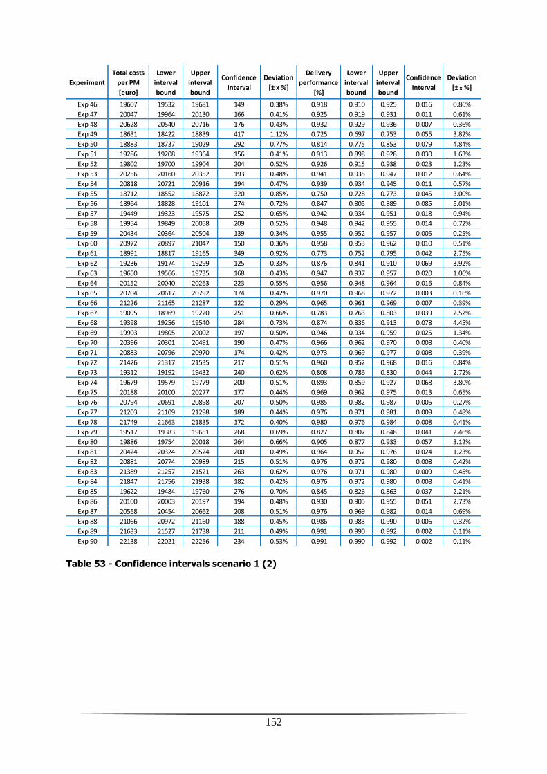
152


Experiment

Total costs

per PM

[euro]

Lower

interval

bound

Upper

interval

bound

Confidence

Interval

Deviation

[± x %]

Delivery

performance

[%]

Lower

interval

bound

Upper

interval

bound

Confidence

Interval

Deviation

[± x %]

Exp 46 19607 19532 19681 149 0.38% 0.918 0.910 0.925 0.016 0.86%

Exp 47 20047 19964 20130 166 0.41% 0.925 0.919 0.931 0.011 0.61%

Exp 48 20628 20540 20716 176 0.43% 0.932 0.929 0.936 0.007 0.36%

Exp 49 18631 18422 18839 417 1.12% 0.725 0.697 0.753 0.055 3.82%

Exp 50 18883 18737 19029 292 0.77% 0.814 0.775 0.853 0.079 4.84%

Exp 51 19286 19208 19364 156 0.41% 0.913 0.898 0.928 0.030 1.63%

Exp 52 19802 19700 19904 204 0.52% 0.926 0.915 0.938 0.023 1.23%

Exp 53 20256 20160 20352 193 0.48% 0.941 0.935 0.947 0.012 0.64%

Exp 54 20818 20721 20916 194 0.47% 0.939 0.934 0.945 0.011 0.57%

Exp 55 18712 18552 18872 320 0.85% 0.750 0.728 0.773 0.045 3.00%

Exp 56 18964 18828 19101 274 0.72% 0.847 0.805 0.889 0.085 5.01%

Exp 57 19449 19323 19575 252 0.65% 0.942 0.934 0.951 0.018 0.94%

Exp 58 19954 19849 20058 209 0.52% 0.948 0.942 0.955 0.014 0.72%

Exp 59 20434 20364 20504 139 0.34% 0.955 0.952 0.957 0.005 0.25%

Exp 60 20972 20897 21047 150 0.36% 0.958 0.953 0.962 0.010 0.51%

Exp 61 18991 18817 19165 349 0.92% 0.773 0.752 0.795 0.042 2.75%

Exp 62 19236 19174 19299 125 0.33% 0.876 0.841 0.910 0.069 3.92%

Exp 63 19650 19566 19735 168 0.43% 0.947 0.937 0.957 0.020 1.06%

Exp 64 20152 20040 20263 223 0.55% 0.956 0.948 0.964 0.016 0.84%

Exp 65 20704 20617 20792 174 0.42% 0.970 0.968 0.972 0.003 0.16%

Exp 66 21226 21165 21287 122 0.29% 0.965 0.961 0.969 0.007 0.39%

Exp 67 19095 18969 19220 251 0.66% 0.783 0.763 0.803 0.039 2.52%

Exp 68 19398 19256 19540 284 0.73% 0.874 0.836 0.913 0.078 4.45%

Exp 69 19903 19805 20002 197 0.50% 0.946 0.934 0.959 0.025 1.34%

Exp 70 20396 20301 20491 190 0.47% 0.966 0.962 0.970 0.008 0.40%

Exp 71 20883 20796 20970 174 0.42% 0.973 0.969 0.977 0.008 0.39%

Exp 72 21426 21317 21535 217 0.51% 0.960 0.952 0.968 0.016 0.84%

Exp 73 19312 19192 19432 240 0.62% 0.808 0.786 0.830 0.044 2.72%

Exp 74 19679 19579 19779 200 0.51% 0.893 0.859 0.927 0.068 3.80%

Exp 75 20188 20100 20277 177 0.44% 0.969 0.962 0.975 0.013 0.65%

Exp 76 20794 20691 20898 207 0.50% 0.985 0.982 0.987 0.005 0.27%

Exp 77 21203 21109 21298 189 0.44% 0.976 0.971 0.981 0.009 0.48%

Exp 78 21749 21663 21835 172 0.40% 0.980 0.976 0.984 0.008 0.41%

Exp 79 19517 19383 19651 268 0.69% 0.827 0.807 0.848 0.041 2.46%

Exp 80 19886 19754 20018 264 0.66% 0.905 0.877 0.933 0.057 3.12%

Exp 81 20424 20324 20524 200 0.49% 0.964 0.952 0.976 0.024 1.23%

Exp 82 20881 20774 20989 215 0.51% 0.976 0.972 0.980 0.008 0.42%

Exp 83 21389 21257 21521 263 0.62% 0.976 0.971 0.980 0.009 0.45%

Exp 84 21847 21756 21938 182 0.42% 0.976 0.972 0.980 0.008 0.41%

Exp 85 19622 19484 19760 276 0.70% 0.845 0.826 0.863 0.037 2.21%

Exp 86 20100 20003 20197 194 0.48% 0.930 0.905 0.955 0.051 2.73%

Exp 87 20558 20454 20662 208 0.51% 0.976 0.969 0.982 0.014 0.69%

Exp 88 21066 20972 21160 188 0.45% 0.986 0.983 0.990 0.006 0.32%

Exp 89 21633 21527 21738 211 0.49% 0.991 0.990 0.992 0.002 0.11%

Exp 90 22138 22021 22256 234 0.53% 0.991 0.990 0.992 0.002 0.11%

153


Experiment

Total costs

per PM

[euro]

Lower

interval

bound

Upper

interval

bound

Confidence

Interval

Deviation

[± x %]

Delivery

performance

[%]

Lower

interval

bound

Upper

interval

bound

Confidence

Interval

Deviation

[± x %]

Exp 01 17947 17624 18270 645 1.80% 0.439 0.408 0.471 0.063 7.17%

Exp 02 17725 17472 17979 507 1.43% 0.546 0.499 0.592 0.094 8.58%

Exp 03 17914 17794 18034 240 0.67% 0.677 0.641 0.712 0.071 5.24%

Exp 04 18353 18290 18416 126 0.34% 0.748 0.732 0.765 0.033 2.22%

Exp 05 18876 18799 18953 154 0.41% 0.777 0.764 0.789 0.025 1.58%

Exp 06 19336 19251 19422 171 0.44% 0.779 0.769 0.789 0.020 1.30%

Exp 07 18024 17710 18339 629 1.75% 0.481 0.447 0.516 0.068 7.09%

Exp 08 17839 17615 18063 448 1.26% 0.582 0.533 0.631 0.098 8.44%

Exp 09 18104 17957 18252 295 0.81% 0.709 0.672 0.747 0.075 5.30%

Exp 10 18494 18443 18544 102 0.27% 0.789 0.771 0.807 0.037 2.31%

Exp 11 19049 18988 19111 124 0.33% 0.811 0.795 0.827 0.031 1.94%

Exp 12 19546 19475 19617 143 0.36% 0.827 0.819 0.836 0.017 1.03%

Exp 13 18060 17747 18373 625 1.73% 0.530 0.494 0.567 0.074 6.94%

Exp 14 17995 17774 18216 441 1.23% 0.630 0.582 0.678 0.096 7.63%

Exp 15 18298 18178 18418 240 0.66% 0.779 0.755 0.803 0.047 3.05%

Exp 16 18745 18645 18844 200 0.53% 0.842 0.831 0.854 0.023 1.34%

Exp 17 19243 19159 19327 168 0.44% 0.861 0.853 0.868 0.015 0.90%

Exp 18 19748 19668 19828 159 0.40% 0.852 0.844 0.860 0.017 0.98%

Exp 19 18173 17879 18468 589 1.62% 0.561 0.528 0.594 0.066 5.86%

Exp 20 18063 17828 18298 470 1.30% 0.679 0.628 0.730 0.101 7.46%

Exp 21 18365 18267 18464 197 0.54% 0.789 0.750 0.827 0.077 4.88%

Exp 22 18748 18680 18816 136 0.36% 0.858 0.843 0.872 0.028 1.66%

Exp 23 19287 19224 19349 124 0.32% 0.874 0.862 0.885 0.024 1.35%

Exp 24 19734 19670 19799 129 0.33% 0.886 0.880 0.892 0.013 0.72%

Exp 25 18272 18032 18511 479 1.31% 0.611 0.573 0.649 0.075 6.15%

Exp 26 18117 17932 18302 370 1.02% 0.708 0.657 0.759 0.102 7.22%

Exp 27 18493 18403 18582 180 0.49% 0.835 0.806 0.863 0.057 3.40%

Exp 28 18932 18867 18997 129 0.34% 0.894 0.883 0.905 0.022 1.21%

Exp 29 19441 19384 19498 114 0.29% 0.913 0.907 0.920 0.013 0.71%

Exp 30 19965 19894 20036 141 0.35% 0.911 0.907 0.914 0.007 0.38%

Exp 31 18348 18050 18646 596 1.62% 0.634 0.600 0.668 0.068 5.38%

Exp 32 18360 18157 18564 407 1.11% 0.739 0.690 0.788 0.099 6.67%

Exp 33 18716 18624 18808 184 0.49% 0.834 0.796 0.873 0.077 4.61%

Exp 34 19159 19095 19223 127 0.33% 0.920 0.912 0.928 0.016 0.90%

Exp 35 19690 19626 19755 129 0.33% 0.928 0.924 0.933 0.009 0.49%

Exp 36 20260 20203 20317 114 0.28% 0.940 0.936 0.943 0.007 0.36%

Exp 37 18533 18293 18773 480 1.30% 0.643 0.612 0.675 0.064 4.95%

Exp 38 18622 18448 18796 348 0.93% 0.744 0.691 0.797 0.106 7.12%

Exp 39 18939 18861 19017 156 0.41% 0.876 0.851 0.902 0.051 2.89%

Exp 40 19411 19320 19502 182 0.47% 0.933 0.924 0.941 0.017 0.92%

Exp 41 19913 19835 19991 157 0.39% 0.942 0.938 0.946 0.008 0.44%

Exp 42 20469 20366 20571 206 0.50% 0.954 0.949 0.958 0.009 0.48%

Exp 43 18599 18345 18854 509 1.37% 0.694 0.659 0.730 0.071 5.10%

Exp 44 18635 18445 18824 379 1.02% 0.790 0.739 0.841 0.103 6.51%

Exp 45 18995 18897 19093 196 0.52% 0.913 0.896 0.930 0.034 1.86%

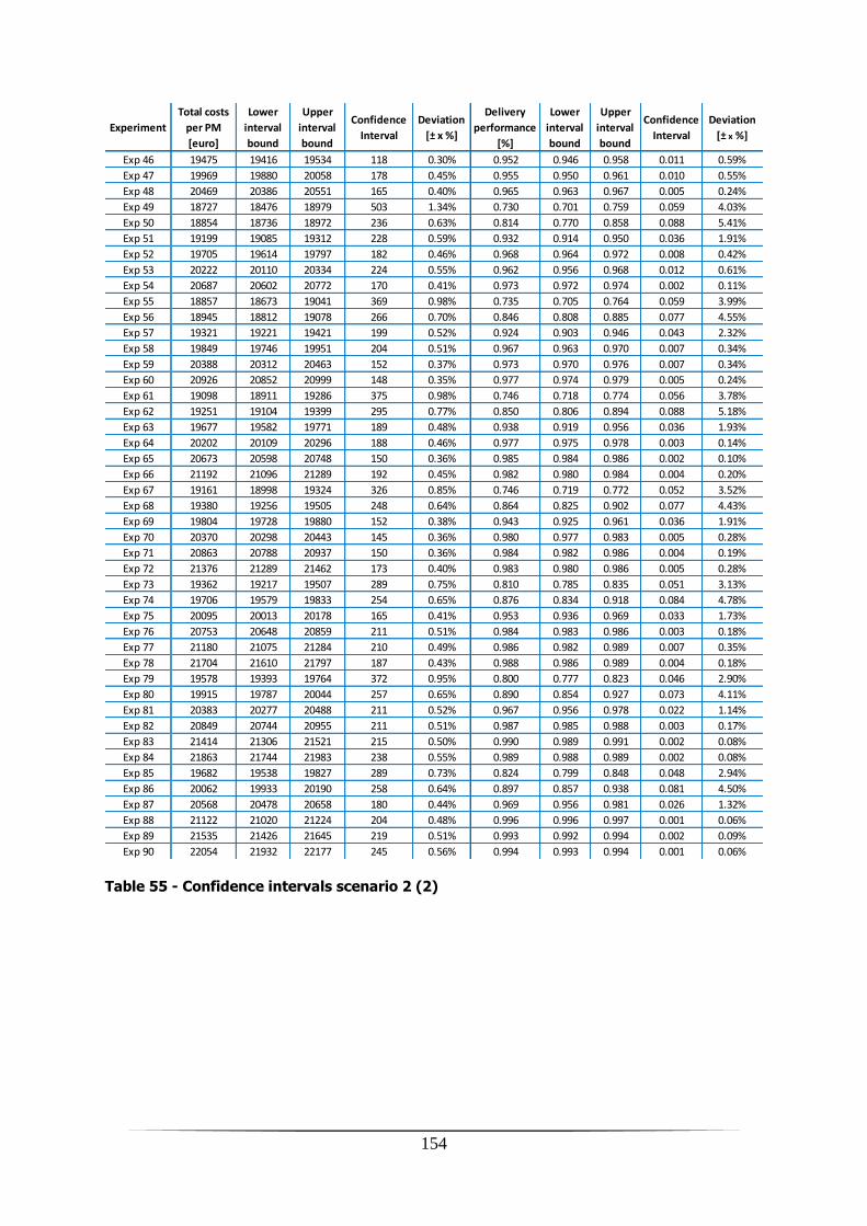
154


Experiment

Total costs

per PM

[euro]

Lower

interval

bound

Upper

interval

bound

Confidence

Interval

Deviation

[± x %]

Delivery

performance

[%]

Lower

interval

bound

Upper

interval

bound

Confidence

Interval

Deviation

[± x %]

Exp 46 19475 19416 19534 118 0.30% 0.952 0.946 0.958 0.011 0.59%

Exp 47 19969 19880 20058 178 0.45% 0.955 0.950 0.961 0.010 0.55%

Exp 48 20469 20386 20551 165 0.40% 0.965 0.963 0.967 0.005 0.24%

Exp 49 18727 18476 18979 503 1.34% 0.730 0.701 0.759 0.059 4.03%

Exp 50 18854 18736 18972 236 0.63% 0.814 0.770 0.858 0.088 5.41%

Exp 51 19199 19085 19312 228 0.59% 0.932 0.914 0.950 0.036 1.91%

Exp 52 19705 19614 19797 182 0.46% 0.968 0.964 0.972 0.008 0.42%

Exp 53 20222 20110 20334 224 0.55% 0.962 0.956 0.968 0.012 0.61%

Exp 54 20687 20602 20772 170 0.41% 0.973 0.972 0.974 0.002 0.11%

Exp 55 18857 18673 19041 369 0.98% 0.735 0.705 0.764 0.059 3.99%

Exp 56 18945 18812 19078 266 0.70% 0.846 0.808 0.885 0.077 4.55%

Exp 57 19321 19221 19421 199 0.52% 0.924 0.903 0.946 0.043 2.32%

Exp 58 19849 19746 19951 204 0.51% 0.967 0.963 0.970 0.007 0.34%

Exp 59 20388 20312 20463 152 0.37% 0.973 0.970 0.976 0.007 0.34%

Exp 60 20926 20852 20999 148 0.35% 0.977 0.974 0.979 0.005 0.24%

Exp 61 19098 18911 19286 375 0.98% 0.746 0.718 0.774 0.056 3.78%

Exp 62 19251 19104 19399 295 0.77% 0.850 0.806 0.894 0.088 5.18%

Exp 63 19677 19582 19771 189 0.48% 0.938 0.919 0.956 0.036 1.93%

Exp 64 20202 20109 20296 188 0.46% 0.977 0.975 0.978 0.003 0.14%

Exp 65 20673 20598 20748 150 0.36% 0.985 0.984 0.986 0.002 0.10%

Exp 66 21192 21096 21289 192 0.45% 0.982 0.980 0.984 0.004 0.20%

Exp 67 19161 18998 19324 326 0.85% 0.746 0.719 0.772 0.052 3.52%

Exp 68 19380 19256 19505 248 0.64% 0.864 0.825 0.902 0.077 4.43%

Exp 69 19804 19728 19880 152 0.38% 0.943 0.925 0.961 0.036 1.91%

Exp 70 20370 20298 20443 145 0.36% 0.980 0.977 0.983 0.005 0.28%

Exp 71 20863 20788 20937 150 0.36% 0.984 0.982 0.986 0.004 0.19%

Exp 72 21376 21289 21462 173 0.40% 0.983 0.980 0.986 0.005 0.28%

Exp 73 19362 19217 19507 289 0.75% 0.810 0.785 0.835 0.051 3.13%

Exp 74 19706 19579 19833 254 0.65% 0.876 0.834 0.918 0.084 4.78%

Exp 75 20095 20013 20178 165 0.41% 0.953 0.936 0.969 0.033 1.73%

Exp 76 20753 20648 20859 211 0.51% 0.984 0.983 0.986 0.003 0.18%

Exp 77 21180 21075 21284 210 0.49% 0.986 0.982 0.989 0.007 0.35%

Exp 78 21704 21610 21797 187 0.43% 0.988 0.986 0.989 0.004 0.18%

Exp 79 19578 19393 19764 372 0.95% 0.800 0.777 0.823 0.046 2.90%

Exp 80 19915 19787 20044 257 0.65% 0.890 0.854 0.927 0.073 4.11%

Exp 81 20383 20277 20488 211 0.52% 0.967 0.956 0.978 0.022 1.14%

Exp 82 20849 20744 20955 211 0.51% 0.987 0.985 0.988 0.003 0.17%

Exp 83 21414 21306 21521 215 0.50% 0.990 0.989 0.991 0.002 0.08%

Exp 84 21863 21744 21983 238 0.55% 0.989 0.988 0.989 0.002 0.08%

Exp 85 19682 19538 19827 289 0.73% 0.824 0.799 0.848 0.048 2.94%

Exp 86 20062 19933 20190 258 0.64% 0.897 0.857 0.938 0.081 4.50%

Exp 87 20568 20478 20658 180 0.44% 0.969 0.956 0.981 0.026 1.32%

Exp 88 21122 21020 21224 204 0.48% 0.996 0.996 0.997 0.001 0.06%

Exp 89 21535 21426 21645 219 0.51% 0.993 0.992 0.994 0.002 0.09%

Exp 90 22054 21932 22177 245 0.56% 0.994 0.993 0.994 0.001 0.06%

155


Experiment

Total costs

per PM

[euro]

Lower

interval

bound

Upper

interval

bound

Confidence

Interval

Deviation

[± x %]

Delivery

performance

[%]

Lower

interval

bound

Upper

interval

bound

Confidence

Interval

Deviation

[± x %]

Exp 01 21225 20597 21853 1256 2.96% 0.143 0.077 0.210 0.133 46.33%

Exp 02 18222 17683 18761 1078 2.96% 0.427 0.373 0.482 0.110 12.84%

Exp 03 17996 17838 18154 316 0.88% 0.641 0.619 0.663 0.044 3.42%

Exp 04 18473 18380 18567 187 0.51% 0.689 0.663 0.714 0.050 3.64%

Exp 05 18965 18849 19081 232 0.61% 0.714 0.697 0.730 0.033 2.33%

Exp 06 19463 19372 19553 181 0.46% 0.744 0.736 0.751 0.015 1.01%

Exp 07 21619 20982 22257 1275 2.95% 0.161 0.082 0.239 0.157 48.82%

Exp 08 18428 17884 18971 1087 2.95% 0.473 0.414 0.532 0.118 12.50%

Exp 09 18193 18079 18307 228 0.63% 0.685 0.652 0.718 0.066 4.83%

Exp 10 18651 18544 18759 215 0.58% 0.742 0.726 0.757 0.030 2.05%

Exp 11 19138 19026 19250 224 0.58% 0.787 0.773 0.800 0.027 1.71%

Exp 12 19715 19616 19814 198 0.50% 0.762 0.750 0.775 0.025 1.67%

Exp 13 21553 20850 22255 1404 3.26% 0.164 0.091 0.237 0.146 44.57%

Exp 14 18481 18021 18941 920 2.49% 0.529 0.466 0.592 0.126 11.94%

Exp 15 18317 18199 18434 234 0.64% 0.733 0.703 0.763 0.060 4.09%

Exp 16 18760 18681 18840 159 0.42% 0.804 0.790 0.819 0.028 1.76%

Exp 17 19298 19197 19399 203 0.53% 0.826 0.818 0.834 0.016 0.95%

Exp 18 19794 19685 19904 218 0.55% 0.794 0.774 0.815 0.041 2.59%

Exp 19 21575 20856 22294 1438 3.33% 0.182 0.104 0.259 0.155 42.57%

Exp 20 18597 18066 19129 1064 2.86% 0.549 0.479 0.618 0.139 12.62%

Exp 21 18440 18327 18552 225 0.61% 0.772 0.747 0.798 0.051 3.28%

Exp 22 18917 18810 19024 214 0.57% 0.823 0.804 0.842 0.037 2.28%

Exp 23 19393 19314 19472 158 0.41% 0.850 0.841 0.859 0.018 1.07%

Exp 24 19892 19816 19968 152 0.38% 0.858 0.853 0.863 0.010 0.56%

Exp 25 21459 20874 22044 1171 2.73% 0.203 0.117 0.290 0.173 42.47%

Exp 26 18779 18345 19214 870 2.32% 0.602 0.528 0.676 0.147 12.24%

Exp 27 18615 18473 18757 284 0.76% 0.794 0.757 0.831 0.074 4.65%

Exp 28 19059 18988 19130 141 0.37% 0.870 0.851 0.889 0.038 2.21%

Exp 29 19508 19447 19570 124 0.32% 0.865 0.854 0.876 0.022 1.27%

Exp 30 20103 20007 20199 193 0.48% 0.864 0.853 0.875 0.022 1.29%

Exp 31 21491 20838 22144 1306 3.04% 0.200 0.119 0.281 0.162 40.42%

Exp 32 18917 18441 19392 951 2.51% 0.623 0.546 0.701 0.156 12.48%

Exp 33 18816 18689 18943 254 0.67% 0.843 0.819 0.867 0.049 2.89%

Exp 34 19192 19145 19238 92 0.24% 0.873 0.854 0.893 0.039 2.23%

Exp 35 19733 19656 19810 154 0.39% 0.894 0.885 0.903 0.018 1.02%

Exp 36 20331 20199 20463 264 0.65% 0.908 0.900 0.916 0.016 0.87%

Exp 37 21702 21121 22283 1163 2.68% 0.224 0.135 0.313 0.177 39.55%

Exp 38 19064 18558 19570 1013 2.66% 0.650 0.568 0.731 0.163 12.52%

Exp 39 18944 18840 19047 207 0.55% 0.870 0.843 0.896 0.053 3.05%

Exp 40 19461 19353 19568 215 0.55% 0.903 0.888 0.919 0.031 1.71%

Exp 41 19987 19875 20099 224 0.56% 0.915 0.906 0.923 0.017 0.94%

Exp 42 20454 20352 20557 205 0.50% 0.918 0.912 0.925 0.013 0.73%

Exp 43 21683 21063 22303 1240 2.86% 0.244 0.159 0.328 0.169 34.74%

Exp 44 19217 18725 19709 984 2.56% 0.692 0.609 0.775 0.166 11.96%

Exp 45 19128 19014 19242 227 0.59% 0.906 0.889 0.923 0.035 1.91%

156


Experiment

Total costs

per PM

[euro]

Lower

interval

bound

Upper

interval

bound

Confidence

Interval

Deviation

[± x %]

Delivery

performance

[%]

Lower

interval

bound

Upper

interval

bound

Confidence

Interval

Deviation

[± x %]

Exp 46 19548 19425 19671 246 0.63% 0.936 0.931 0.941 0.010 0.54%

Exp 47 20031 19926 20136 211 0.53% 0.934 0.926 0.941 0.015 0.79%

Exp 48 20539 20407 20672 265 0.64% 0.935 0.930 0.940 0.011 0.56%

Exp 49 21429 20885 21973 1088 2.54% 0.282 0.195 0.369 0.175 31.01%

Exp 50 19284 18888 19679 791 2.05% 0.722 0.640 0.804 0.164 11.39%

Exp 51 19321 19206 19436 230 0.59% 0.909 0.887 0.931 0.045 2.45%

Exp 52 19735 19641 19829 188 0.48% 0.950 0.943 0.956 0.012 0.66%

Exp 53 20254 20158 20350 192 0.47% 0.950 0.944 0.957 0.013 0.67%

Exp 54 20791 20668 20914 246 0.59% 0.943 0.940 0.947 0.007 0.39%

Exp 55 21505 20905 22106 1201 2.79% 0.313 0.229 0.397 0.168 26.91%

Exp 56 19387 19037 19737 700 1.80% 0.757 0.676 0.838 0.163 10.76%

Exp 57 19501 19388 19613 225 0.58% 0.948 0.938 0.957 0.019 1.00%

Exp 58 19986 19881 20090 208 0.52% 0.958 0.952 0.964 0.012 0.63%

Exp 59 20444 20357 20531 174 0.43% 0.956 0.949 0.962 0.014 0.72%

Exp 60 20929 20816 21042 225 0.54% 0.946 0.936 0.956 0.020 1.07%

Exp 61 21612 21110 22115 1005 2.33% 0.303 0.213 0.394 0.182 29.90%

Exp 62 19643 19257 20029 772 1.96% 0.763 0.681 0.846 0.165 10.84%

Exp 63 19714 19599 19829 231 0.59% 0.953 0.943 0.962 0.019 0.99%

Exp 64 20169 20070 20268 199 0.49% 0.966 0.960 0.972 0.012 0.63%

Exp 65 20769 20629 20910 281 0.68% 0.966 0.959 0.972 0.013 0.69%

Exp 66 21322 21185 21459 274 0.64% 0.974 0.971 0.977 0.005 0.27%

Exp 67 21574 21115 22033 919 2.13% 0.332 0.248 0.416 0.168 25.23%

Exp 68 19767 19382 20151 769 1.94% 0.770 0.686 0.854 0.167 10.87%

Exp 69 19946 19837 20055 218 0.55% 0.949 0.932 0.965 0.032 1.71%

Exp 70 20329 20209 20450 242 0.59% 0.966 0.960 0.972 0.013 0.65%

Exp 71 20834 20753 20915 162 0.39% 0.982 0.980 0.984 0.004 0.19%

Exp 72 21415 21316 21514 198 0.46% 0.980 0.977 0.983 0.006 0.29%

Exp 73 21579 21083 22075 993 2.30% 0.367 0.288 0.447 0.159 21.58%

Exp 74 20023 19720 20327 607 1.52% 0.805 0.726 0.883 0.156 9.72%

Exp 75 20203 20114 20291 177 0.44% 0.955 0.938 0.972 0.034 1.77%

Exp 76 20655 20557 20753 196 0.48% 0.979 0.972 0.986 0.014 0.73%

Exp 77 21205 21109 21301 192 0.45% 0.987 0.984 0.989 0.005 0.25%

Exp 78 21675 21548 21802 254 0.59% 0.985 0.984 0.987 0.003 0.15%

Exp 79 21615 21148 22082 934 2.16% 0.426 0.349 0.502 0.154 18.04%

Exp 80 20213 19826 20601 775 1.92% 0.803 0.717 0.890 0.173 10.78%

Exp 81 20331 20243 20418 175 0.43% 0.954 0.938 0.970 0.032 1.69%

Exp 82 20894 20803 20985 181 0.43% 0.987 0.986 0.988 0.003 0.13%

Exp 83 21382 21256 21507 251 0.59% 0.982 0.978 0.986 0.008 0.40%

Exp 84 21874 21766 21982 216 0.49% 0.985 0.983 0.987 0.004 0.21%

Exp 85 21760 21278 22243 965 2.22% 0.437 0.361 0.512 0.152 17.35%

Exp 86 20372 20061 20683 622 1.53% 0.832 0.755 0.909 0.154 9.24%

Exp 87 20611 20519 20703 183 0.44% 0.959 0.942 0.977 0.035 1.83%

Exp 88 20996 20892 21101 208 0.50% 0.986 0.983 0.988 0.005 0.27%

Exp 89 21549 21453 21645 193 0.45% 0.986 0.984 0.988 0.004 0.20%

Exp 90 22095 21969 22221 252 0.57% 0.990 0.989 0.992 0.004 0.18%

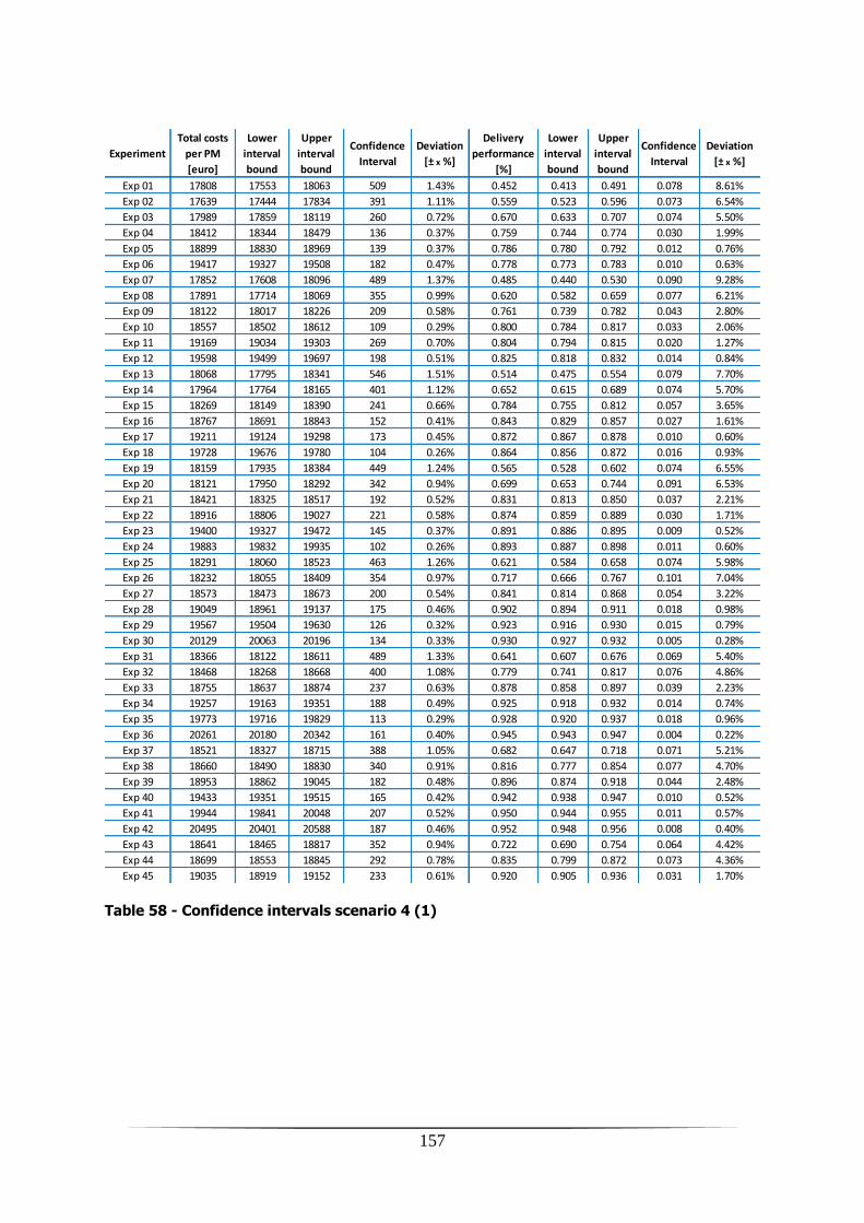
157


Experiment

Total costs

per PM

[euro]

Lower

interval

bound

Upper

interval

bound

Confidence

Interval

Deviation

[± x %]

Delivery

performance

[%]

Lower

interval

bound

Upper

interval

bound

Confidence

Interval

Deviation

[± x %]

Exp 01 17808 17553 18063 509 1.43% 0.452 0.413 0.491 0.078 8.61%

Exp 02 17639 17444 17834 391 1.11% 0.559 0.523 0.596 0.073 6.54%

Exp 03 17989 17859 18119 260 0.72% 0.670 0.633 0.707 0.074 5.50%

Exp 04 18412 18344 18479 136 0.37% 0.759 0.744 0.774 0.030 1.99%

Exp 05 18899 18830 18969 139 0.37% 0.786 0.780 0.792 0.012 0.76%

Exp 06 19417 19327 19508 182 0.47% 0.778 0.773 0.783 0.010 0.63%

Exp 07 17852 17608 18096 489 1.37% 0.485 0.440 0.530 0.090 9.28%

Exp 08 17891 17714 18069 355 0.99% 0.620 0.582 0.659 0.077 6.21%

Exp 09 18122 18017 18226 209 0.58% 0.761 0.739 0.782 0.043 2.80%

Exp 10 18557 18502 18612 109 0.29% 0.800 0.784 0.817 0.033 2.06%

Exp 11 19169 19034 19303 269 0.70% 0.804 0.794 0.815 0.020 1.27%

Exp 12 19598 19499 19697 198 0.51% 0.825 0.818 0.832 0.014 0.84%

Exp 13 18068 17795 18341 546 1.51% 0.514 0.475 0.554 0.079 7.70%

Exp 14 17964 17764 18165 401 1.12% 0.652 0.615 0.689 0.074 5.70%

Exp 15 18269 18149 18390 241 0.66% 0.784 0.755 0.812 0.057 3.65%

Exp 16 18767 18691 18843 152 0.41% 0.843 0.829 0.857 0.027 1.61%

Exp 17 19211 19124 19298 173 0.45% 0.872 0.867 0.878 0.010 0.60%

Exp 18 19728 19676 19780 104 0.26% 0.864 0.856 0.872 0.016 0.93%

Exp 19 18159 17935 18384 449 1.24% 0.565 0.528 0.602 0.074 6.55%

Exp 20 18121 17950 18292 342 0.94% 0.699 0.653 0.744 0.091 6.53%

Exp 21 18421 18325 18517 192 0.52% 0.831 0.813 0.850 0.037 2.21%

Exp 22 18916 18806 19027 221 0.58% 0.874 0.859 0.889 0.030 1.71%

Exp 23 19400 19327 19472 145 0.37% 0.891 0.886 0.895 0.009 0.52%

Exp 24 19883 19832 19935 102 0.26% 0.893 0.887 0.898 0.011 0.60%

Exp 25 18291 18060 18523 463 1.26% 0.621 0.584 0.658 0.074 5.98%

Exp 26 18232 18055 18409 354 0.97% 0.717 0.666 0.767 0.101 7.04%

Exp 27 18573 18473 18673 200 0.54% 0.841 0.814 0.868 0.054 3.22%

Exp 28 19049 18961 19137 175 0.46% 0.902 0.894 0.911 0.018 0.98%

Exp 29 19567 19504 19630 126 0.32% 0.923 0.916 0.930 0.015 0.79%

Exp 30 20129 20063 20196 134 0.33% 0.930 0.927 0.932 0.005 0.28%

Exp 31 18366 18122 18611 489 1.33% 0.641 0.607 0.676 0.069 5.40%

Exp 32 18468 18268 18668 400 1.08% 0.779 0.741 0.817 0.076 4.86%

Exp 33 18755 18637 18874 237 0.63% 0.878 0.858 0.897 0.039 2.23%

Exp 34 19257 19163 19351 188 0.49% 0.925 0.918 0.932 0.014 0.74%

Exp 35 19773 19716 19829 113 0.29% 0.928 0.920 0.937 0.018 0.96%

Exp 36 20261 20180 20342 161 0.40% 0.945 0.943 0.947 0.004 0.22%

Exp 37 18521 18327 18715 388 1.05% 0.682 0.647 0.718 0.071 5.21%

Exp 38 18660 18490 18830 340 0.91% 0.816 0.777 0.854 0.077 4.70%

Exp 39 18953 18862 19045 182 0.48% 0.896 0.874 0.918 0.044 2.48%

Exp 40 19433 19351 19515 165 0.42% 0.942 0.938 0.947 0.010 0.52%

Exp 41 19944 19841 20048 207 0.52% 0.950 0.944 0.955 0.011 0.57%

Exp 42 20495 20401 20588 187 0.46% 0.952 0.948 0.956 0.008 0.40%

Exp 43 18641 18465 18817 352 0.94% 0.722 0.690 0.754 0.064 4.42%

Exp 44 18699 18553 18845 292 0.78% 0.835 0.799 0.872 0.073 4.36%

Exp 45 19035 18919 19152 233 0.61% 0.920 0.905 0.936 0.031 1.70%

158


Experiment

Total costs

per PM

[euro]

Lower

interval

bound

Upper

interval

bound

Confidence

Interval

Deviation

[± x %]

Delivery

performance

[%]

Lower

interval

bound

Upper

interval

bound

Confidence

Interval

Deviation

[± x %]

Exp 46 19511 19419 19603 184 0.47% 0.942 0.929 0.954 0.026 1.37%

Exp 47 19995 19909 20081 172 0.43% 0.964 0.962 0.965 0.003 0.17%

Exp 48 20570 20490 20650 160 0.39% 0.966 0.965 0.967 0.002 0.12%

Exp 49 18844 18662 19027 365 0.97% 0.732 0.705 0.760 0.056 3.80%

Exp 50 18904 18720 19089 369 0.98% 0.840 0.799 0.880 0.080 4.78%

Exp 51 19264 19168 19360 192 0.50% 0.924 0.904 0.944 0.040 2.17%

Exp 52 19720 19638 19802 164 0.42% 0.966 0.962 0.971 0.008 0.43%

Exp 53 20212 20132 20293 161 0.40% 0.971 0.969 0.974 0.005 0.28%

Exp 54 20753 20688 20819 130 0.31% 0.974 0.972 0.976 0.004 0.23%

Exp 55 19008 18815 19200 385 1.01% 0.791 0.765 0.816 0.051 3.20%

Exp 56 19127 18964 19289 325 0.85% 0.853 0.811 0.894 0.083 4.86%

Exp 57 19413 19316 19509 192 0.50% 0.937 0.918 0.955 0.037 1.97%

Exp 58 19875 19794 19957 164 0.41% 0.965 0.958 0.972 0.014 0.74%

Exp 59 20413 20320 20505 185 0.45% 0.980 0.979 0.982 0.002 0.13%

Exp 60 20920 20823 21016 193 0.46% 0.976 0.974 0.979 0.005 0.28%

Exp 61 19110 18956 19265 309 0.81% 0.778 0.755 0.802 0.047 3.01%

Exp 62 19362 19225 19499 273 0.71% 0.909 0.886 0.932 0.046 2.52%

Exp 63 19697 19574 19821 247 0.63% 0.952 0.935 0.968 0.033 1.73%

Exp 64 20203 20085 20321 236 0.59% 0.977 0.973 0.982 0.009 0.45%

Exp 65 20690 20593 20787 194 0.47% 0.983 0.982 0.984 0.003 0.13%

Exp 66 21217 21127 21306 179 0.42% 0.984 0.983 0.985 0.002 0.10%

Exp 67 19256 19079 19432 352 0.91% 0.835 0.814 0.857 0.043 2.59%

Exp 68 19543 19413 19674 261 0.67% 0.889 0.853 0.926 0.074 4.14%

Exp 69 19842 19744 19940 197 0.50% 0.953 0.937 0.969 0.033 1.71%

Exp 70 20423 20346 20500 154 0.38% 0.980 0.975 0.984 0.009 0.45%

Exp 71 20868 20790 20946 155 0.37% 0.985 0.984 0.986 0.002 0.11%

Exp 72 21358 21277 21439 162 0.38% 0.984 0.983 0.985 0.002 0.11%

Exp 73 19491 19365 19616 250 0.64% 0.856 0.838 0.873 0.034 2.01%

Exp 74 19758 19635 19882 247 0.62% 0.903 0.867 0.938 0.071 3.92%

Exp 75 20210 20136 20283 147 0.36% 0.958 0.942 0.974 0.032 1.65%

Exp 76 20647 20559 20735 176 0.43% 0.986 0.982 0.990 0.008 0.39%

Exp 77 21207 21089 21325 236 0.56% 0.991 0.990 0.992 0.002 0.08%

Exp 78 21679 21572 21787 215 0.50% 0.992 0.992 0.993 0.002 0.08%

Exp 79 19646 19501 19790 289 0.74% 0.853 0.839 0.868 0.029 1.70%

Exp 80 20006 19882 20131 249 0.62% 0.915 0.882 0.949 0.067 3.66%

Exp 81 20358 20257 20459 202 0.50% 0.967 0.953 0.981 0.028 1.42%

Exp 82 20790 20681 20898 217 0.52% 0.984 0.979 0.989 0.010 0.53%

Exp 83 21389 21299 21480 181 0.42% 0.995 0.993 0.996 0.003 0.14%

Exp 84 21908 21810 22006 196 0.45% 0.994 0.993 0.995 0.002 0.10%

Exp 85 19833 19687 19979 292 0.74% 0.879 0.863 0.894 0.031 1.77%

Exp 86 20129 20004 20254 250 0.62% 0.931 0.905 0.957 0.052 2.77%

Exp 87 20525 20412 20638 226 0.55% 0.969 0.957 0.981 0.024 1.22%

Exp 88 21009 20909 21110 202 0.48% 0.991 0.990 0.993 0.003 0.15%

Exp 89 21527 21429 21624 196 0.45% 0.991 0.990 0.993 0.003 0.15%

Exp 90 22000 21902 22097 196 0.44% 0.993 0.992 0.995 0.002 0.11%

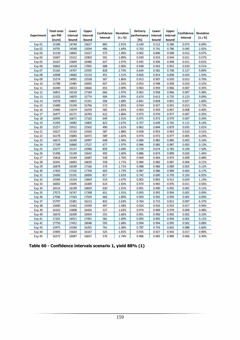
159

Table 60 - Confidence intervals scenario 1, yield 88% (1)

Experiment

Total costs

per PM

[euro]

Lower

interval

bound

Upper

interval

bound

Confidence

Interval

Deviation

[± x %]

Delivery

performance

[%]

Lower

interval

bound

Upper

interval

bound

Confidence

Interval

Deviation

[± x %]

Exp 01 15186 14744 15627 883 2.91% 0.549 0.512 0.586 0.073 6.69%

Exp 02 14791 14548 15034 486 1.64% 0.763 0.741 0.786 0.045 2.92%

Exp 03 15130 14842 15417 575 1.90% 0.902 0.896 0.908 0.012 0.67%

Exp 04 15607 15312 15903 591 1.89% 0.939 0.933 0.944 0.011 0.57%

Exp 05 16167 15849 16486 637 1.97% 0.942 0.936 0.948 0.011 0.61%

Exp 06 16662 16318 17005 688 2.06% 0.948 0.943 0.953 0.010 0.51%

Exp 07 15181 14767 15595 828 2.73% 0.644 0.581 0.708 0.127 9.89%

Exp 08 14908 14682 15133 451 1.51% 0.826 0.814 0.838 0.024 1.43%

Exp 09 15274 14991 15558 567 1.86% 0.913 0.907 0.920 0.013 0.70%

Exp 10 15788 15485 16092 607 1.92% 0.953 0.948 0.958 0.010 0.52%

Exp 11 16340 16013 16666 653 2.00% 0.963 0.959 0.966 0.007 0.35%

Exp 12 16851 16518 17184 666 1.97% 0.962 0.958 0.966 0.007 0.38%

Exp 13 15322 14870 15774 904 2.95% 0.674 0.613 0.735 0.123 9.09%

Exp 14 15078 14825 15331 506 1.68% 0.841 0.828 0.855 0.027 1.60%

Exp 15 15480 15194 15766 572 1.85% 0.934 0.927 0.941 0.013 0.72%

Exp 16 15966 15674 16259 585 1.83% 0.963 0.959 0.967 0.008 0.40%

Exp 17 16477 16171 16783 612 1.86% 0.973 0.970 0.977 0.007 0.35%

Exp 18 16995 16671 17320 649 1.91% 0.975 0.972 0.979 0.007 0.34%

Exp 19 15393 14982 15805 823 2.67% 0.707 0.649 0.765 0.115 8.14%

Exp 20 15257 15012 15502 490 1.61% 0.862 0.844 0.879 0.035 2.01%

Exp 21 15627 15333 15920 587 1.88% 0.958 0.953 0.963 0.010 0.51%

Exp 22 16178 15883 16472 589 1.82% 0.974 0.972 0.977 0.005 0.24%

Exp 23 16673 16349 16997 648 1.94% 0.984 0.982 0.985 0.003 0.16%

Exp 24 17199 16860 17537 677 1.97% 0.986 0.985 0.987 0.003 0.13%

Exp 25 15577 15157 15996 839 2.69% 0.729 0.674 0.783 0.109 7.50%

Exp 26 15396 15149 15642 493 1.60% 0.886 0.874 0.899 0.026 1.44%

Exp 27 15818 15549 16087 538 1.70% 0.969 0.964 0.974 0.009 0.48%

Exp 28 16341 16063 16620 558 1.71% 0.984 0.982 0.987 0.004 0.21%

Exp 29 16878 16590 17166 576 1.71% 0.988 0.986 0.989 0.002 0.12%

Exp 30 17403 17102 17704 603 1.73% 0.987 0.986 0.989 0.003 0.17%

Exp 31 15600 15191 16009 817 2.62% 0.742 0.690 0.793 0.103 6.92%

Exp 32 15584 15324 15843 519 1.67% 0.902 0.892 0.912 0.020 1.13%

Exp 33 16002 15695 16309 614 1.92% 0.970 0.965 0.976 0.011 0.56%

Exp 34 16514 16199 16829 630 1.91% 0.991 0.990 0.992 0.002 0.11%

Exp 35 17073 16747 17398 651 1.91% 0.993 0.992 0.994 0.002 0.09%

Exp 36 17596 17263 17929 666 1.89% 0.993 0.992 0.994 0.002 0.09%

Exp 37 15797 15381 16213 832 2.63% 0.764 0.715 0.812 0.097 6.37%

Exp 38 15690 15442 15939 497 1.58% 0.924 0.916 0.933 0.017 0.94%

Exp 39 16162 15898 16426 527 1.63% 0.974 0.969 0.978 0.009 0.48%

Exp 40 16676 16399 16954 555 1.66% 0.991 0.990 0.992 0.002 0.10%

Exp 41 17201 16911 17491 581 1.69% 0.993 0.992 0.994 0.002 0.11%

Exp 42 17750 17452 18048 595 1.68% 0.994 0.994 0.995 0.002 0.08%

Exp 43 15975 15594 16355 761 2.38% 0.787 0.743 0.832 0.088 5.60%

Exp 44 15905 15643 16167 525 1.65% 0.935 0.927 0.943 0.017 0.90%

Exp 45 16372 16087 16657 570 1.74% 0.986 0.983 0.989 0.006 0.30%

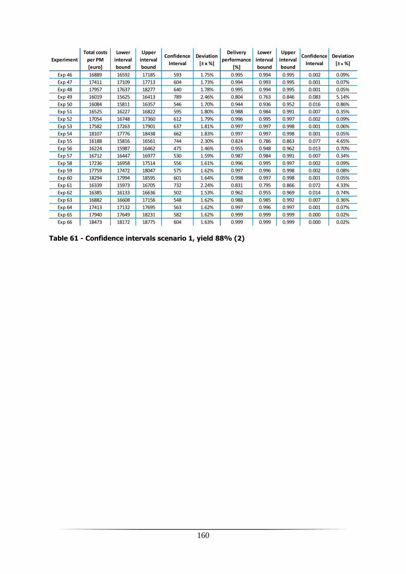
160

Table 61 - Confidence intervals scenario 1, yield 88% (2)

Experiment

Total costs

per PM

[euro]

Lower

interval

bound

Upper

interval

bound

Confidence

Interval

Deviation

[± x %]

Delivery

performance

[%]

Lower

interval

bound

Upper

interval

bound

Confidence

Interval

Deviation

[± x %]

Exp 46 16889 16592 17185 593 1.75% 0.995 0.994 0.995 0.002 0.09%

Exp 47 17411 17109 17713 604 1.73% 0.994 0.993 0.995 0.001 0.07%

Exp 48 17957 17637 18277 640 1.78% 0.995 0.994 0.995 0.001 0.05%

Exp 49 16019 15625 16413 789 2.46% 0.804 0.763 0.846 0.083 5.14%

Exp 50 16084 15811 16357 546 1.70% 0.944 0.936 0.952 0.016 0.86%

Exp 51 16525 16227 16822 595 1.80% 0.988 0.984 0.991 0.007 0.35%

Exp 52 17054 16748 17360 612 1.79% 0.996 0.995 0.997 0.002 0.09%

Exp 53 17582 17263 17901 637 1.81% 0.997 0.997 0.998 0.001 0.06%

Exp 54 18107 17776 18438 662 1.83% 0.997 0.997 0.998 0.001 0.05%

Exp 55 16188 15816 16561 744 2.30% 0.824 0.786 0.863 0.077 4.65%

Exp 56 16224 15987 16462 475 1.46% 0.955 0.948 0.962 0.013 0.70%

Exp 57 16712 16447 16977 530 1.59% 0.987 0.984 0.991 0.007 0.34%

Exp 58 17236 16958 17514 556 1.61% 0.996 0.995 0.997 0.002 0.09%

Exp 59 17759 17472 18047 575 1.62% 0.997 0.996 0.998 0.002 0.08%

Exp 60 18294 17994 18595 601 1.64% 0.998 0.997 0.998 0.001 0.05%

Exp 61 16339 15973 16705 732 2.24% 0.831 0.795 0.866 0.072 4.33%

Exp 62 16385 16133 16636 502 1.53% 0.962 0.955 0.969 0.014 0.74%

Exp 63 16882 16608 17156 548 1.62% 0.988 0.985 0.992 0.007 0.36%

Exp 64 17413 17132 17695 563 1.62% 0.997 0.996 0.997 0.001 0.07%

Exp 65 17940 17649 18231 582 1.62% 0.999 0.999 0.999 0.000 0.02%

Exp 66 18473 18172 18775 604 1.63% 0.999 0.999 0.999 0.000 0.02%

161

Table 62 - Scenario 1, yield 100%

Experiment

Total costs

per PM

[euro]

Lower

interval

bound

Upper

interval

bound

Confidence

Interval

Deviation

[± x %]

Delivery

performance

[%]

Lower

interval

bound

Upper

interval

bound

Confidence

Interval

Deviation

[± x %]

Exp 01 14355 14326 14384 58 0.20% 0.279 0.277 0.281 0.004 0.65%

Exp 02 13126 12934 13318 384 1.46% 0.556 0.519 0.593 0.074 6.69%

Exp 03 13403 13371 13435 64 0.24% 0.830 0.807 0.854 0.047 2.86%

Exp 04 13894 13862 13925 63 0.23% 0.922 0.917 0.927 0.010 0.54%

Exp 05 14254 14051 14457 405 1.42% 0.442 0.374 0.510 0.136 15.39%

Exp 06 13207 13026 13389 362 1.37% 0.640 0.600 0.680 0.080 6.23%

Exp 07 13480 13465 13496 31 0.11% 0.891 0.870 0.913 0.044 2.45%

Exp 08 13967 13965 13969 5 0.02% 0.967 0.964 0.970 0.005 0.27%

Exp 09 14327 14155 14499 344 1.20% 0.469 0.402 0.535 0.134 14.25%

Exp 10 13397 13229 13565 336 1.25% 0.708 0.664 0.752 0.088 6.22%

Exp 11 13797 13768 13827 59 0.21% 0.934 0.918 0.950 0.032 1.72%

Exp 12 14298 14271 14325 54 0.19% 0.984 0.982 0.987 0.005 0.24%

Exp 13 14338 14164 14511 346 1.21% 0.495 0.431 0.559 0.128 12.91%

Exp 14 13500 13341 13658 316 1.17% 0.764 0.717 0.810 0.093 6.12%

Exp 15 13831 13811 13851 40 0.14% 0.961 0.950 0.973 0.023 1.20%

Exp 16 14328 14315 14342 27 0.09% 0.993 0.991 0.994 0.003 0.16%

Exp 17 14387 14228 14545 317 1.10% 0.519 0.458 0.580 0.122 11.79%

Exp 18 13651 13500 13801 301 1.10% 0.806 0.757 0.856 0.099 6.13%

Exp 19 14042 13994 14090 97 0.34% 0.977 0.967 0.987 0.020 1.00%

Exp 20 14549 14500 14599 98 0.34% 0.998 0.998 0.999 0.001 0.04%

Exp 21 14463 14318 14608 290 1.00% 0.539 0.480 0.598 0.118 10.93%

Exp 22 13801 13664 13938 273 0.99% 0.835 0.785 0.885 0.100 5.99%

Exp 23 14208 14195 14221 27 0.09% 0.982 0.975 0.990 0.015 0.78%

Exp 24 14717 14704 14731 27 0.09% 0.999 0.999 1.000 0.000 0.02%

Exp 25 14498 14370 14626 256 0.88% 0.564 0.509 0.619 0.110 9.75%

Exp 26 13961 13840 14083 243 0.87% 0.863 0.814 0.912 0.098 5.65%

Exp 27 14407 14382 14431 49 0.17% 0.988 0.982 0.994 0.012 0.59%

Exp 28 14918 14893 14942 50 0.17% 1.000

Exp 29 14532 14430 14634 204 0.70% 0.590 0.539 0.642 0.103 8.74%

Exp 30 14104 13996 14213 218 0.77% 0.883 0.835 0.931 0.095 5.39%

Exp 31 14558 14533 14583 50 0.17% 0.993 0.990 0.997 0.007 0.35%

Exp 32 15068 15043 15092 49 0.16% 1.000

Exp 33 14603 14513 14693 180 0.62% 0.621 0.573 0.669 0.096 7.69%

Exp 34 14254 14157 14352 195 0.68% 0.902 0.857 0.946 0.089 4.96%

Exp 35 14719 14705 14733 28 0.10% 0.997 0.995 0.999 0.003 0.16%

Exp 36 15233 15209 15257 48 0.16% 0.993 0.992 0.994 0.002 0.09%

Documents

FACULTY OF MECHANICAL, MARITIME AND MATERIALS Delft