Factors Influencing Emerging Market Central Banks’ Decision to Intervene in Foreign

Exchange Markets

Matthew Malloy

WP/13/70

© 2013 International Monetary Fund WP/13/70

IMF Working Paper

Office of the Executive Director for the United States (OEDUA)

Factors Influencing Emerging Market Central Banks’ Decision to Intervene in Foreign Exchange Markets

Prepared by Matthew Malloy1

Authorized for distribution by Meg Lundsager

March 15, 2013

Abstract Using panel data for 15 economies from 2001-12, I identify determinants of central bank foreign exchange intervention in emerging markets (“EMs”) with flexible to moderately managed exchange rates. Similar to other studies, I find that central banks tend to “lean against the wind,” buying/selling more foreign exchange in response to greater short-run and medium-run appreciation/depreciation pressures. The panel structure provides a framework to test whether other macroeconomic variables influence the different rates of reserve accumulation between economies. In testing other variables, I find evidence of both precautionary and external competitiveness motives for reserve accumulation. JEL Classification Numbers: F31 Keywords: foreign exchange intervention, international reserves Author’s E-Mail Address: mmalloy@imf.org

1 I would like to thank Trevor Reeve for his guidance throughout the process of conducting this study. I would also like to thank Shaghil Ahmed, Steve Phillips, Jonathan Ostry, Luis Catao, Rex Ghosh, James Roaf, Charalambos Tsangarides, Joe Gagnon, Bill Lindquist, and Jay Shambaugh for their useful comments.

2 The opinions expressed in this paper are the author’s only and do not necessarily represent those of the U.S. Treasury Department, Office of the U.S. Executive Director at the IMF, or the International Monetary Fund, and should not be reported as such.

This Working Paper should not be reported as representing the views of the IMF.2 The views expressed in this Working Paper are those of the author(s) and do not necessarily represent those of the IMF or IMF policy. Working Papers describe research in progress by the author(s) and are published to elicit comments and to further debate.

2

Contents I. Introduction ........................................................................................................................... 3 II. Data ...................................................................................................................................... 5 III. Estimation Technique ......................................................................................................... 9 IV. Results and Interpretation ................................................................................................... 9

A. Baseline Model ................................................................................................................ 9 B. What Drives Differences in Rates of Reserve Accumulation? ...................................... 12 C. Changing Motivations? .................................................................................................. 14 D. Other Determinants? ...................................................................................................... 15

V. Robustneess Checks ........................................................................................................... 16

A. Intervention Data Quality............................................................................................... 16B. Controls for INT and Δe Simultaneity Bias ................................................................... 17

VI. Conclusion ........................................................................................................................ 17 Figures 1. Growth of Foreign Exchange Reserves ................................................................................ 5 Tables - Regression Output 1. Determinants of FX Intervention ........................................................................................ 19 2. Time Subperiods ................................................................................................................. 20 3. Other Reserve Adequacy Metrics ....................................................................................... 21 4. Interactions between Independent Variables ...................................................................... 22 5. FX Intervention Data Robustness Tests .............................................................................. 23 6. Controls betweeen INT and ∆e Simultaneity Bias ............................................................. 24 Appendices 1. Notes on Foreign Exchange Intervention Data Utilized in Model ..................................... 25 References ............................................................................................................................... 27

3

I. INTRODUCTION

The purpose of this paper is to identify determinants of foreign exchange intervention in emerging markets (“EMs”) over the last decade. This study focuses on EMs that have sufficiently flexible exchange rate regimes, for which the decision to intervene is not required for maintenance of the exchange rate regime (such as with a fixed exchange rate, basket peg, crawling peg, etc.). Thus, for these EM central banks, a decision to purchase or sell foreign exchange, and how much, is a choice, and thus may be influenced by a number of factors. This paper does not attempt to answer whether FX intervention is effective in influencing the exchange rate. For a thorough discussion on this topic see Ostry 2011. There are three main determinants for intervention cited in the literature and by practitioners:

1) Smoothing short-run fluctuations of the exchange rate, particularly in cases when the exchange rate is overshooting or assessed by authorities to be misaligned.

2) Accumulation of foreign exchange reserves for precautionary purposes.

3) Accumulation of foreign exchange reserves for competitiveness reasons.

The determinants are likely not mutually exclusive, as there may be more than one reason to intervene at a given point in time. For example, a central bank may choose to opportunistically purchase reserves for precautionary purposes during periods of appreciation to both smooth exchange rate volatility and add to reserves. Similarly, a central bank may buy foreign exchange reserves for precautionary purposes and for competitiveness reasons, since purchasing reserves could have this dual effect. Regarding the first determinant, there is considerable empirical evidence from the literature that central banks tend to purchase (sell) foreign exchange to stem short-run appreciation (depreciation) pressures, i.e. “lean against the wind.” These exchange rate pressures are either modeled as a deviation from trend or a monthly/daily change. Much of the literature focuses on advanced economies, including Australia (Kim and Sheen 2002), Japan (Kim and Sheen 2005, Frenkel et al. 2004, and Germany and the U.S. (Almekinders and Eijffinger 1996). Also some recent studies have focused on emerging markets, including Turkey (Ozlu and Prokhorov 2007) and Georgia (Aslanidi 2007). All of these studies find evidence that central banks lean against the wind. The limitation of these approaches is that they mainly account for the intervention response to short-run, fast-moving variables and utilize single-country equations, and thus do not account for why the rate of reserve accumulation differs between EMs.

Regarding the second and third determinants, much of the literature focuses on identifying why EMs have different stock levels of foreign exchange reserves. Most recently, Ghosh et al. (2012) develop a panel OLS model using annual data from 1980-2010, categorizing independent variables into three main areas: vulnerability to current account shocks, vulnerability to capital account shocks, and mercantilist motivations, to explain the stock level of foreign exchange reserves. They find that variables in all three areas are significant

4

determinants of the stock level of reserves, though motivations seem to shift over time. Ghosh to some degree builds off of Obstfeld (2007) and Bastoure (2009), which includes many of the same current account and capital account independent variables as Ghosh, but do not include any variables for mercantilist motives. For a thorough discussion on this topic see Ghosh (2012).

The limitation of this approach is that the stock of reserves reflects past behavior, and thus non-contemporaneous determinants may not fully account for why a central bank has accumulated reserves previously. For example, a country such as Japan, while holding a large stock of reserves, accumulated the majority of them over eight years ago. Thus, present day indicators of Japan’s openness, exchange rate level, asset price volatility, etc., may not account accurately for its reserve stock.

In this study, in order to mitigate the limitations of both approaches, I develop a model that is a hybrid of two above approaches – one that includes both short-run exchange rate pressures as well as broader macroeconomic variables to account for the rate of foreign exchange accumulation within and between economies. I try to answer the question: why is an EM intervening in foreign exchange markets now, and why is it intervening differently from other EMs?

Using a similar approach, Adler and Tovar (2012) introduce some slower moving variables into their estimates of single country central bank foreign exchange intervention reaction functions, including: a measure of exchange rate misalignment (based on an average of the three IMF CGER methodologies) and reserve adequacy ratios (reserves-to short-term debt and reserves-to-M2). They find that that the exchange rate misalignment variable has a positive coefficient (i.e. more overvaluation leads to an increase in net FX purchases) and is statistically significant in six out of ten EMs modeled. They generally did not find the reserve adequacy ratios to be statistically significant.

Utilizing aspects of Adler and Tovar (2012), I take their approach in a different direction – by using a panel structure and introducing additional slower moving macroeconomic variables. Much of literature on intervention determinants stresses the need to evaluate determinants on a country-by-country basis, to take into account individual central bank preferences and tendencies. While single country equations may be more tailored for an individual country, a panel structure can also be useful, by providing information on why behavior may be different across EMs. Since the general direction of EM central bank reserves has been upward, it is particularly relevant to include variables in a panel structure that may account for why rates of accumulation are different – while also maintaining faster-moving variables in the equation as controls.

5

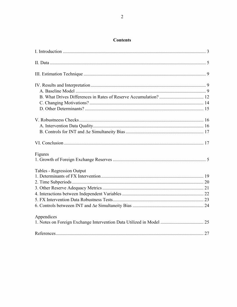
To attempt to understand the determinants of foreign exchange intervention for these EMs, I use a panel least squares model with AR1 residuals and heteroskedasticity corrected (robust) standard errors (White). I include monthly data for 15 EM cross-sections3. All EMs in the panel have flexible or moderately managed exchange rates. In addition to modeling short-run exchange rate pressures, I include broader macroeconomic variables, such as: the real effective exchange rate relative to a medium-term trend, the export sector as a share of GDP, reserve adequacy metrics, and year-over-year CPI inflation change, in my baseline specification. In additional specifications, I conduct a set of interactions between the independent variables, to identify possible joint effects, as well as introduce additional independent variables as tests.

II. DATA

Selection of EMs Used in Sample The most important condition for EMs used in the sample is that their exchange rate was sufficiently flexible in the entire observation period, such that a central bank’s decision to intervene is independent of the degree of pressure on the exchange rate. In other words, the exchange rate regime does not require the central bank to buy/sell foreign exchange reserves to maintain a certain level of the exchange rate, such as with a peg, a crawling peg, or even a highly managed float. A second condition was that intervention data was available or could be estimated on a monthly basis.4

3 Brazil, Colombia, Indonesia, India, Israel, Korea, Mexico, Peru, Philippines, Poland, Russia, South Africa, Taiwan, Thailand, and Turkey

4 The only EM not selected for this reason was Chile, as it was not clear how much foreign exchange was contributed to their sovereign wealth funds on a monthly basis, particularly at the early part of the time series.

Figure 1. Growth of foreign exchange reserves in EMs over the last decade. Foreign exchange reserves as a percentage of GDP of the fifteen EMs in the study have increased significantly since 2001, but the rates of accumulation have been quite different.

Sources: Haver, central bank websites

10%

14%

18%

22%

26%

Jan

-01

Jan

-03

Jan

-05

Jan

-07

Jan

-09

Jan

-11

FX Reserves as % of GDP: 15 EMs in the Study

0%

2%

4%

6%

8%

Taiw

an

Thai

lan

d

Ru

ssia

Ph

ilip

pin

es

Per

u

Isra

el

Ind

ia

Ko

rea

Bra

zil

Po

lan

d

Ind

on

esia

Sou

th A

fric

a

Turk

ey

Co

lom

bia

Mex

ico

Average Annual Increase in Foreign Exchange Reserves (% of GDP): 2001-2011

6

All EMs that met the above criteria and that were above $150 billion in nominal GDP in 2011 were included in the sample. Dependent Variable For the purposes of this study, total monthly intervention is a sum of the net change of the central banks’ position in the spot market )( SInt and the net change of its position in the

forward market )( FInt , divided by a interpolated monthly GDP series (derived from a quarterly, seasonally adjusted GDP series in U.S. dollars)

GDP

IntIntInt FS

Intervention is expressed in U.S. dollars. One of the limitations is that spot foreign exchange intervention data is not available for some EMs. The following indicates what intervention data is used for each EM5:

Published Intervention Data: Brazil, Colombia, India, Israel, Mexico, Peru, Russia (after 2007), and Turkey.

Monthly Change in Reserves with Valuation Changes Stripped Out by Central Bank: Korea, Philippines, Poland, Taiwan (after October 2003), and Thailand.

Monthly Change in Reserves with Valuation Changes Stripped Out by Author with Known Annual Currency Composition of Reserves: Russia (before 2008) and South Africa. In these countries, the central bank has published currency composition of reserves, and I use this data to strip out exchange rate valuation changes. Other valuation changes, such as mark to market changes are not adjusted.6

Monthly Change in Reserves with Valuation Changes Stripped Out by Author with Unknown Annual Currency Composition of Reserves: Indonesia and Taiwan (before November 2003). For these economies, I strip out exchange rate valuation changes based on the average currency composition of reserves in EMs.7

Fourteen EMs (all except Taiwan) publish their monthly interventions in foreign exchange forward markets in their publicly available reserve template submission to the IMF. 5 For more information on the foreign exchange intervention data utilized please see Appendix I.

6 Generally, valuation changes associated with foreign exchange rate changes have the largest impact on the a month-to-month basis. Market valuation and other valuation changes do not tend to impact reserves as much.

7 Based on the IMF’s Currency Composition of Foreign Exchange Reserves (COFER) data.

7

The mean of

 for all EMs in the sample is 2.4 percent of monthly GDP and the median is 1.2 percent.  In the full d. Independent Variables – Short-run exchange rate pressures Short-run exchange rate pressures in the model are measured by the change in nominal U.S. dollar bilateral exchange rate compared to the previous month (“Δe”). Using Δe as an explanatory variable likely introduces an endogeneity problem. Intervention responds to Δe, but Δe is also affected by intervention. To control for this likely simultaneity bias between and Δe in my baseline specification, I use the one-month lag of Δe on the right-hand side of the equation8. While using the lagged Δe eliminates the simultaneity bias, there is potential that it introduces an omitted variable bias in the equation, since it likely that central banks intervene in foreign exchange markets in response to exchange rate pressures in the current month (and not just in the previous month). As a proxy for Δe, I use the monthly change in the VIX9. The VIX is correlated with broad market risk sentiment and capital flows to emerging markets, which tend to be the most volatile determinant of monthly exchange rate movements in these markets. The VIX does not capture well economy-specific determinants of monthly exchange rate changes however. As such, I provide an alternate specification without the VIX variable as a robustness check. As the main purpose of the paper is not to estimate a coefficient for Δe – but instead to estimate the impacts of the slower moving macroeconomic variables on INT (while controlling for Δe) – the above solution to the simultaneity bias problem is sufficient. Using a two-stage least squares model with instrumental variables would allow for an estimate of Δe, but identifying good instruments is difficult. As a robustness check, I estimate the equation using a TSLS model, using the change in the VIX and Δe for other economies in the model as instruments. I find that there was little difference between the coefficients on the slower moving macroeconomic variables in the baseline model and TSLS. Independent Variable – REER relative to 5-year average

8 The bias to the coefficient on Δe is likely upward. An increase in Δe is estimated to result in an increase in

. But, an increase in INT likely also results in a decrease in Δe. Because the actual amount of exchange rate change is decreased by intervention, the model interprets this lower of amount of exchange rate change as the amount that is associated with the change in INT. However, the amount of total exchange rate pressure necessary to result in the change in INT is in fact larger, which means that absent the simultaneity bias, the coefficient on Δe would be lower.

9 The monthly change in the VIX is calculated:

8

To model a central banks’ response to medium-term real exchange rate pressures I use the percent change between the current value of the real effective exchange rate10 and its rolling five-year average as a independent variable (“RER”):

))(ln()ln( 60... ttt REERavgREERRER

In order to eliminate any simultaneity bias with INT or collinearity with Δe(-1), I use a two-month lag of RER. Independent Variable – Exports as a share of GDP To determine whether a larger export sector impacts a central bank’s decision to intervene in foreign exchange markets – I use monthly goods exports as a share of GDP as a regressor (“ " .  It was expected that   would be positively associated with  because a central bank may want to hold more precautionary reserves with a larger external trade sector and may also be more concerned about the impact of appreciation on competiveness. Utilizing the panel structure of the model, this variable is included primarily to explain the different rates of foreign exchange intervention between EMs. Independent Variable – Reserve Adequacy Dummies To test whether reserve adequacy impacts a central bank’s decision to intervene, I construct two reserve adequacy dummies based upon the IMF reserve adequacy metric11. The IMF metric is the desired level of reserves constructed as function of possible liability drains during a crisis. Identified drains are estimated as possible annual percentage losses of: short-term debt, other portfolio liabilities, export income, and M2. By dividing the actual level of reserves by the metric we can quantify the level of reserve adequacy. The IMF determines that EMs with reserves that are 100-150% of the metric have an adequate level. In the first dummy variable (RAD1), if in a given month12 reserves are above 150% of the metric than that month is given a 1, otherwise a 0. In the second variable (RAD2), if reserves are below 100% of the metric than that month is given a 1. 10 BIS, CPI-based real effective exchange rate

11 The IMF reserve adequacy metric methodology is described in a 2011 IMF paper “Assessing Reserve Adequacy.” The metric is constructed in the following method for countries with floating exchange rates – Metric = 30% of External Short-term Debt + 10% of Other External Liabilities + 5% of M2 + 5% of exports. Exports are in annual terms.

12 The reserve adequacy metric is constructing using annual data. To create monthly data, I interpolate the annual data linearly.

9

Independent Variable – Inflation The rate of inflation (“π”) is measured as the year-on-year rate of change of the monthly CPI. It was expected that π would have a negative association with . Higher/lower π could make a central bank more reluctant to buy/sell foreign exchange, as they may want the exchange rate to help smooth the inflation trend. Higher/lower π could also translate to higher/lower sterilization costs13. There may also be some countervailing effects in which π has a positive association with

.  Higher π  and the associated higher nominal interest rates  could attract carry trade capital inflowfor commodity producers.

III. ESTIMATION TECHNIQUE

I use a panel least squares model with AR1 residuals and heteroskedasticity corrected standard errors (White); 15 EM cross-sections; and monthly data from 2001 to 201214. There are no cross-section or time-fixed effects applied. I use a dummy variable for the global financial crisis period, which in the model is from May 2008 to December 2008. As such, the baseline equation is:

1 2 3 4 5 5 6 7( 1) 1 2 (1)INT c vix e RER ExG RAD RAD crisisdum AR

IV. RESULTS AND INTERPRETATION

A. Baseline Model

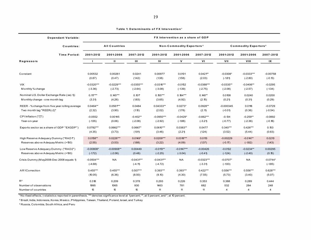
Table 1 indicates the output from the model for the full sample as well as output from sub-periods (2001-2006 and 2007-2012) and different EM groups (commodity and non-commodity exporters). Except for the VIX and EXGDP (exports to GDP), none of the independent variables in the baseline specification are statistically significant for the sub-group of commodity exporters in the dataset. VIX

13 This effect may be mitigated to the degree that EM central bank’s sterilization tools have an interest rate below the policy rate.

14 The sample period ends in February 2012.

10

A 10% m-o-m increase in the VIX (eg. 20 to 22) is associated with a 0.32% of GDP decrease in INT. The coefficients are similar and statistically significant for both non-commodity and commodity producers. If the VIX is indeed picking up non-country specific exchange rate pressures associated with global risk sentiment – then we can assume that the VIX is proxying reasonably well for the current month exchange rate change, given that the coefficient has the expected sign and is statistically significant. For example, as global investor sentiment becomes more risk averse, the VIX increases, capital tends to flow out of most EMs putting pressure on exchange rates to depreciate. Thus, the VIX is expected to have a negative coefficient if proxying well for short-run exchange rate changes. Short-run Exchange Rate Pressure A 1% m-o-m appreciation of Δe(-1) is associated with a 0.16% of GDP increase in INT for non-commodity producers. The coefficient on Δe(-1) is fairly stable across time periods, however is not statistically significant for commodity producers. I tested whether there is an asymmetric response when Δe(-1) is positive compared to when it is negative, but found no evidence of this. This does not imply that intervention is balanced between purchases and sales, as is indicated by the descriptive statistics of INT, just that the positive inclination of INT is driven by other variables in the equation. These output confirms results in previous studies that central banks tend to buy and sell foreign exchange to lean against the wind of short-term exchange rate movements. REER For non-commodity producers, a real effective exchange rate (with a two month lag, RER(-2)) that is 10% more appreciated than its five-year rolling average is associated with a 0.43% of GDP increase in INT compared to a level that is equal to its 5-year rolling average. For commodity producers the coefficient on RER(-2) is not statistically significant. Similar to Δe(-1), I tested whether there is an asymmetric response when RER(-2) is positive (appreciated) compared to when it is negative (depreciated), but found no evidence of this. The positive and statistically significant coefficient on the REER variable for non-commodity exporters may suggest that central banks have an eye on competitiveness when they make their decision to intervene. For example, an EM whose REER(-2) is 20% above its 5-year average is expected to increase its net FX purchases by 1.75 percentage points of GDP per month more than an EM whose REER is 20% below its five-year average, holding other factors constant. The positive coefficients on the short-run and medium-run exchange rate variables could also be interpreted as central banks opportunistically buying foreign exchange reserves for precautionary reasons while appreciation pressures are stronger. This is more likely for the

11

short-run exchange rate variables since the REER variable is at a two-month lag, and an appreciation of the REER relative to its medium-term average (lagged by two months) is not necessarily consistent with appreciation pressures in the very short-run. Inflation For non-commodity exporters, a 1% increase in year-on-year CPI inflation is associated with a 0.1% of GDP decrease in INT for the full sample, but the coefficient increases sharply to 0.7% of GDP in the 2007-2012 time period15. The coefficient on CPI is not statistically significant for commodity exporters. The negative and statistically significant coefficient on the 12-month CPI inflation change, suggests that intervention decisions may be influenced by the price level. An EM with 12% y-o-y inflation is expected to decrease its net FX purchases by 1.0% percentage points of GDP per month compared to an EM with 2% y-o-y inflation. The rationale for this, as previously noted, is that an EM with higher inflation may prefer to allow more appreciation (less depreciation) by reducing its net foreign exchange purchases, which could help reduce inflation. Exports as a percentage of GDP A 10% increase in exports as a share of GDP (“EXGDP”) is associated with 0.78% of GDP increase in INT. Thus, a country such as Korea, which has an export/GDP ratio of 53% is estimated to purchase on average 1.6% of GDP more in foreign exchange reserves per month compared to Mexico, which has an export/GDP ratio of 32%. EXGDP is statistically significant for both commodity and non-commodity exporters. One might conclude from this result that an EM with a larger export sector relative to other EMs’ export sectors may determine that they need a higher level of precautionary reserves to absorb external shocks, and thus purchase more foreign exchange on a monthly basis. One might also consider that an EM with a larger export sector would have greater motivation to intervene for external competitiveness reasons. I examine these two motivations in greater detail below. Reserves Adequacy Dummies The dummy variable for periods when EMs have high reserve adequacy (“RAD1”) has a positive coefficient and is statistically significant for non-commodity exporters, but not for commodity exporters. Months in which central banks have a high reserve adequacy level (over 150% of the IMF reserve metric) are associated with an increase of 1.6% of GDP in net foreign exchange purchases per month.

15 Part of this sharp increase may be due to an anomalous period during the global financial crisis (second half of 2008) when y-o-y inflation remained quite high following the commodity boom, but depreciation pressure intensified strongly.

12

Conversely, the dummy variable for periods when EMs have low reserve adequacy (“RAD2”) has a negative coefficient, and also is only statistically significant for non-commodity exporters. Months in which central banks have a low reserve adequacy level (below 100% of the IMF reserve metric) are associated with a decrease of 0.6% of GDP in net foreign exchange purchases per month. The positive coefficient on the high reserve adequacy dummy variable (RAD1) suggests that in periods when EMs have more than adequate reserves, as measured by the IMF reserve adequacy metric, they still tend to buy more foreign exchange reserves, on net, than their peers. Additionally, the negative coefficient on the low reserve adequacy dummy variable (RAD2), suggests that EMs which have inadequate levels of foreign exchange reserves do not try or are not able to “catch up” to the suggested adequacy level. If precautionary demand for reserves, as defined by the IMF reserve adequacy metric, were a main consideration in the intervention decision, one would expect the signs on these coefficients to be reversed, such that EMs calibrate their foreign exchange reserve purchases/sales to target the mid-range of the IMF metric. B. What Drives Differences in Rates of Reserve Accumulation?

We now augment the model to gather further information to answer the question as to what are the main factors that cause the different rates of reserve accumulation over time. The exchange rate variables in the model have a mean of roughly zero, and thus explain very little of the difference in rates of accumulation between EMs. We have seen that EMs with persistently high inflation tend to purchase fewer reserves than their peers with lower inflation – however, this does not account for much of difference in rates of reserve accumulation. To further test whether reserve adequacy is a main driver of intervention, in separate specifications (Table 3), I test four additional measures of reserve adequacy – reserves/GDP; reserves/GDP relative to the EM average; reserves/imports; and the IMF reserve adequacy metric. In these specifications, I drop EXGDP (exports to GDP) and the reserve adequacy dummies from the equation to avoid multicollinearty concerns. I lag all four measures by one month to control for any endogeneity. The results in Table 3 indicate that all four measures have a positive coefficient and are statistically significant, consistent with baseline result. These model results suggest the EMs with high relative levels of foreign exchange reserves tend to continue to accumulate reserves at a faster rate than their peers even when taking into account relative levels of traditional reserve adequacy determinants (trade sector size, M2, and external liabilities). The reserve adequacy dummies explain a moderate amount of difference in reserve accumulation between economies in the model, but not in the direction one would expect based on a precautionary motive. EXGDP (exports to GDP) is the most important independent variable in the equation for explaining the different rates of reserve accumulation. For example, according to output in

13

the baseline specification, an EM with an exports to GDP level of 60% is expected on average to purchase 4% of GDP more of net foreign exchange than an EM with an export ratio of 10%. Over time, assuming similar rates of nominal GDP growth, this much higher rate of accumulation would likely lead to persistently higher level of reserves. To understand better whether EXGDP has a positive coefficient as a result of precautionary or mercantilist demand for foreign exchange reserves, I interacted it with the other independent variables in the equation.

EXGDP interacted with the dummy variable for high reserve adequacy has a statistically significant positive coefficient, suggesting that EMs with higher reserve levels are more sensitive to their export level as it relates to intervention. If precautionary demand was the main reason why EXGDP (non-interacted) had a positive coefficient, one would expect the coefficient on this interaction to be negative, as EMs with already high levels of reserve adequacy should be less sensitive to EXGDP in their intervention decision.

I also found that EXGDP interacted with Δe(-1) had a statistically significant positive coefficient, indicating that EMs with higher EXGDP are more sensitive to short-run exchange rate movements.

I did not find that that EXGDP interacted with the REER to have a statistically significant coefficient.

The above results suggest that EXGDP’s positive coefficient is related to non-precautionary demand for reserves. However, other considerations suggest the positive coefficient on EXGDP may be explained better by precautionary demand. In general, EXGDP is highly correlated with other reserve adequacy metrics such as M2/GDP and short-term debt to GDP. One rationale for this is that EMs that are more open and have more financial sector development hold more foreign exchange reserves for precautionary purposes to mitigate their higher potential exposure to balance of payment pressures. Replacing EXGDP with other reserve adequacy metrics, M2/GDP or short-term debt to GDP (STDG) in equation (see table 3) results in these new independent variables having positive coefficients that are statistically significant, though still not as robust an indicator as EXGDP. It is hard to argue that having a higher relative level of M2/GDP or STDG increases external competitiveness concerns for EMs. On the one hand, it’s possible that M2/GDP and STDG could be proxying for EXGDP given their high correlations. But its also possible that the positive coefficient on EXGDP is related to building reserves for precautionary purposes, and the positive coefficient on the interaction between EXGDP and RAD1 (high reserve adequacy dummy) may be simply due to the fact that many EMs have a different views from the IMF reserve adequacy metric on what their precautionary level of reserves should be. Additionally, the coefficient on EXGDP may be driven in part by the higher “replacement rate” of reserve accumulation that is required for a central bank with a higher exports to GDP

14

level to target a level of reserve in relation to the level of exports (assuming such a target exists). On balance, I suspect the positive association between EXGDP and net foreign exchange purchases is indicative of both precautionary and competitiveness motives. While some ambiguity remains, these tests together provide some evidence that the competitiveness motive is a determinant for foreign exchange rate intervention, alongside short-run smoothing and precautionary motives. In particular, the higher rate of reserve accumulation in EMs that already have higher reserve adequacy is not well explained by the precautionary motive. The positive and statistically significant coefficients on the REER and EXGDP variables provide additional pieces of supporting evidence that the competiveness motive may impact the foreign exchange intervention decision. Regarding the positive coefficient on reserve adequacy metrics, it may be that a few EMs that have accumulated reserves at a faster rate and hold more reserves have skewed the association between intervention and reserve adequacy, such that it appears in the data that reserve adequacy is not a main determinant. For EMs with lower relative levels of reserve adequacy their primary motivation for the accumulation of reserves may be for precautionary purposes, but the actions of some central banks that are accumulating reserves at a much faster rate obscure this motivation in the model. It is also quite possible that EMs have very different views on what is an adequate level of reserves for their specific circumstances. If common reserve adequacy metrics do not explain well the precautionary demand for reserve accumulation among EMs, than the positive, statistically significant coefficients on the reserve metric independent variables could be proxying for unexplained precautionary factors. In other words, EMs with high observed reserve adequacy measures may systematically have larger but unmeasured precautionary needs. Further, the unmeasured elements may not be common across economies. Finally, as mentioned in the introduction, the reasons for different rates of reserve accumulation between EMs need not be mutually exclusive. Some EMs may accumulate reserves for precautionary reasons, but also welcome the potential competitiveness gains that this policy could provide. This could result in a bias of EMs accumulating reserves towards (or above) the upper limits of their own precautionary need estimates. C. Changing Motivations?

The results between the 2001-06 and 2007-12 periods exhibit some important differences, particularly for non-commodity exporters. The positive coefficients on the REER and CPI variables are much larger in 2007-12 relative to 2001-06, suggesting increased sensitivity of foreign exchange intervention to these variables for non-commodity exporters. The positive coefficients on the reserve adequacy dummies steadily lose statistical significance over the ten-year data set. Table 2 disaggregates the data even further – into four time periods. In the 2001-06 period, there were greater differences of economic stability among EMs. A handful of EMs were stable economically and accumulating reserves rapidly above standard reserve adequacy metrics, while a significant group of EMs were either experiencing a

15

financial crisis or recovering from one. In this post-Asian crisis environment, many EMs may have accumulated reserves at whatever rate they could, both for precautionary reasons and for competitiveness reasons. This could explain the positive coefficient on the high reserve adequacy dummy in this period, as a handful of EMs could accumulate very rapidly, while a number of other EMs could not accumulate at all, despite having inadequate reserves. The “accumulate whenever possible” mentality may also explain the lower economic significance of the REER and inflation coefficients in this period. In the 2007-2012 period, there were more EMs on an even footing in terms of macroeconomic stability and reserve adequacy. The average level of the IMF reserve adequacy metric for the EMs in the sample rises from 122% in the 2001-06 period to 168% in the 2007-12 period (100-150 is the suggested adequacy range). The high reserve adequacy dummy may lose significance in this period because the majority of EMs in this period are now above the 150% threshold16. In the 2007-12 period, EM central banks may have become more sophisticated in their intervention strategies – intervening more/less forcefully when the REER appreciated/depreciated from its medium-term average, and more/less forcefully when inflation was low/high to help smooth the inflation trend. D. Other Determinants?

Below is a list of other independent variables that I considered incorporating in the model, but were not included in the final specification:

I completed a full set of interactions between the independent variables in the equation. The interactions - (EXGDP*RAD1) and (EXGDP* Δe(-1)) – I have already mentioned earlier in the paper. I also found that the interaction – (Δe and RAD1) had statistically significant positive coefficient, suggesting that EMs with higher reserve adequacy are more sensitive to short-run exchange rate movements. (To limit multicollinearty with the inclusion of multiple interaction terms, I took the following approach: in a separate equation regressed the interacted term on its components (A*B = c +βA + βB + u) and then took the residual series from this equation and included it in my main intervention equation.)

I tested whether CDS, as a proxy for country risk was significant in the equation. It did have a statistically significant negative coefficient, but was also highly correlated with a number of other variables in the equation, in particular, inflation – so, its was difficult to isolate its effect. The negative association between CDS and net foreign exchange purchases may be because EMs that are at high risk have difficulty accumulating reserves. The negative coefficient on CDS may also be proxying for the higher cost of holding reserves as financing costs rise.

16 The reserve adequacy metric (non-dummy version) if placed separately in the equation (sans EXGDP and reserve adequacy dummies) remains positive and statistically significant in this period.

16

Manufacturing exports as a share of GDP (MANEX) was a less robust indicator than just total exports to GDP (though both are significant at a 99 percent level). Commodity exports to GDP had roughly the same coefficient as MANEX, but were not statistically significant.

I constructed a variable of manufacturing exports to the United States as percentage of GDP (MEUS), with the hypothesis that this could reduce the amount of foreign exchange purchases by central banks (while controlling for EXGDP). The correlation between MEUS and EXGDP is fairly low (0.14). I did find that the coefficient on MEUS was negative and statistically significant when added to the main specification of my equation. However, MEUS lost all statistical significance once Mexico was taken out of the data set.

Monthly changes of the NEER or REER with a one month lag were not as robust independent variables as the monthly changes of the nominal bilateral exchange rate with the U.S. dollar (Δe). I also tried a deviation of the nominal bilateral exchange rate from a very short-run trend (using an HP filter), but this was also not as robust as Δe.

I created dummy variables for periods six month prior to a presidential election and the 2-year period after a financial crisis. Neither variable was statistically significant.

I found that central banks’ policy rates behaved in a similar way to the inflation variables in the equation, given the two series’ strong correlation. However, I found that the policy rate was a less robust determinant compared to inflation.

Per capita GDP and total population were both statistically insignificant when included in the equation.

There was no evidence of a seasonal pattern for foreign exchange intervention in the full data set once all the main independent variables were included in the equation.

V. ROBUSTNESS CHECKS

A. Intervention Data Quality

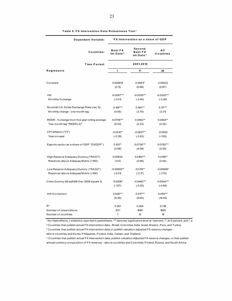
There is likely some degree of error introduced into the model resulting from measurement of the dependent variable – foreign exchange intervention divided by GDP. As noted in the data section, for four out of the fifteen EMs, I have estimated intervention by stripping out exchange rate valuation changes from monthly changes in the stock of foreign exchange reserves. Table 5 provides output from the model using different sets of EMs according to the quality of their foreign exchange intervention data. In column 1, I include only EMs that publish

17

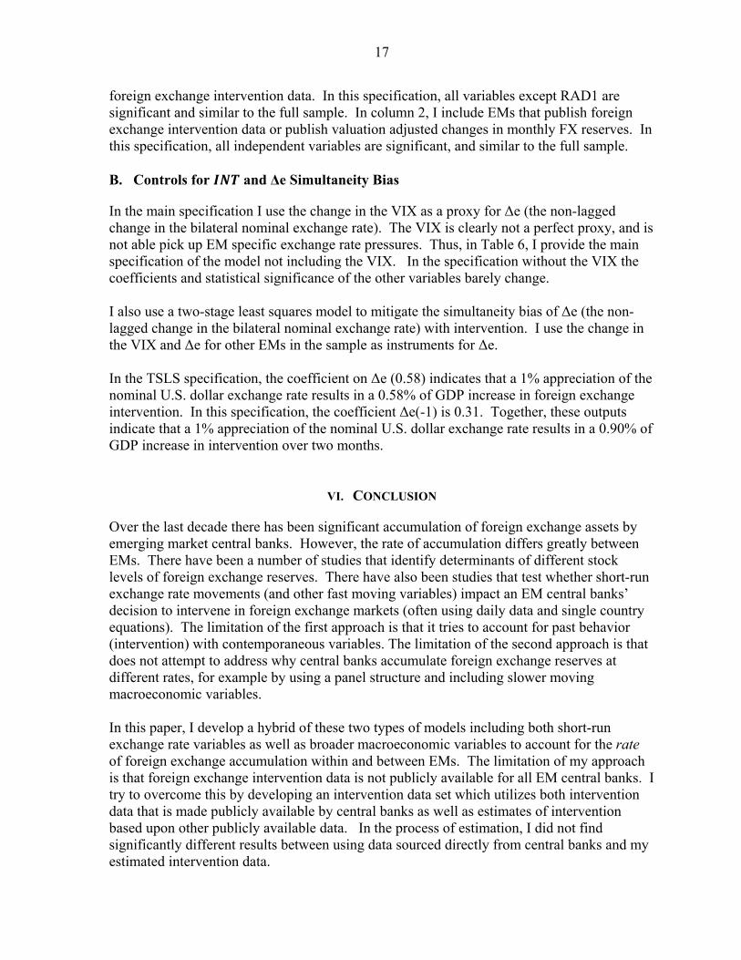
foreign exchange intervention data. In this specification, all variables except RAD1 are significant and similar to the full sample. In column 2, I include EMs that publish foreign exchange intervention data or publish valuation adjusted changes in monthly FX reserves. In this specification, all independent variables are significant, and similar to the full sample. B. Controls for and Δe Simultaneity Bias

In the main specification I use the change in the VIX as a proxy for Δe (the non-lagged change in the bilateral nominal exchange rate). The VIX is clearly not a perfect proxy, and is not able pick up EM specific exchange rate pressures. Thus, in Table 6, I provide the main specification of the model not including the VIX. In the specification without the VIX the coefficients and statistical significance of the other variables barely change. I also use a two-stage least squares model to mitigate the simultaneity bias of Δe (the non-lagged change in the bilateral nominal exchange rate) with intervention. I use the change in the VIX and Δe for other EMs in the sample as instruments for Δe. In the TSLS specification, the coefficient on Δe (0.58) indicates that a 1% appreciation of the nominal U.S. dollar exchange rate results in a 0.58% of GDP increase in foreign exchange intervention. In this specification, the coefficient Δe(-1) is 0.31. Together, these outputs indicate that a 1% appreciation of the nominal U.S. dollar exchange rate results in a 0.90% of GDP increase in intervention over two months.

VI. CONCLUSION

Over the last decade there has been significant accumulation of foreign exchange assets by emerging market central banks. However, the rate of accumulation differs greatly between EMs. There have been a number of studies that identify determinants of different stock levels of foreign exchange reserves. There have also been studies that test whether short-run exchange rate movements (and other fast moving variables) impact an EM central banks’ decision to intervene in foreign exchange markets (often using daily data and single country equations). The limitation of the first approach is that it tries to account for past behavior (intervention) with contemporaneous variables. The limitation of the second approach is that does not attempt to address why central banks accumulate foreign exchange reserves at different rates, for example by using a panel structure and including slower moving macroeconomic variables. In this paper, I develop a hybrid of these two types of models including both short-run exchange rate variables as well as broader macroeconomic variables to account for the rate of foreign exchange accumulation within and between EMs. The limitation of my approach is that foreign exchange intervention data is not publicly available for all EM central banks. I try to overcome this by developing an intervention data set which utilizes both intervention data that is made publicly available by central banks as well as estimates of intervention based upon other publicly available data. In the process of estimation, I did not find significantly different results between using data sourced directly from central banks and my estimated intervention data.

18

The model output provides some evidence that the competitiveness motive is a determinant for foreign exchange rate intervention, alongside short-run smoothing and precautionary motives. In particular, the higher rate of reserve accumulation among EMs that already have higher reserve adequacy is not well explained by the precautionary motive. The positive and statistically significant coefficients on the REER and EXGDP variables provide additional pieces of supporting evidence that the competiveness motive may impact the foreign exchange intervention decision. An area not well explored in this paper is how the type and quality of the monetary policy framework impacts the decision to intervene in foreign exchange markets. As many EM central banks move towards more sophisticated monetary frameworks with better tools to deal with the monetary impact of capital flows, they may be less inclined to use foreign exchange intervention or hold high levels of reserves. These differences in approaches/ability of EM central banks in dealing with exchange rate pressure cycles are difficult to quantify, but could be interesting area for further research in understanding the different rates of reserve accumulation between economies. It might also be interesting to test the role of capital controls on foreign exchange intervention decisions.

19

D ependant Variable:

C o untries:

T ime P erio d: 2001-2012 2001-2006 2007-2012 2001-2012 2001-2006 2007-2012 2001-2012 2001-2006 2007-2012

R egresso rs I II III IV V VI VII VIII IX

Constant 0.00532 0.00261 0.0241 0.00977 0.0101 0.0421** -0.0308* -0.0333*** -0.00758

(0.87) (0.47) (1.42) (1.38) (1.58) (2.03) (-1.81) (-2.80) (-0.13)

VIX -0.0320*** -0.0229*** -0.0355*** -0.0316*** -0.0152 -0.0388*** -0.0335** -0.0406** -0.0295

M onthly % change (-3.36) (-2.73) (-2.64) (-3.08) (-1.39) (-2.75) (-2.08) (-2.57) (-1.34)

Nominal U.S. Dollar Exchange Rate (∆e(-1)) 0.117*** 0.145*** 0.101* 0.155*** 0.184*** 0.148** 0.0108 0.0240 0.0200

M onthly change - one month lag (3.31) (4.26) (1.83) (3.65) (4.92) (2.15) (0.21) (0.31) (0.29)

REER - % change from five year ro lling average 0.0464** 0.0561*** 0.0484 0.04333** 0.0273* 0.0928** -0.000345 0.0118 -0.0729

Two month lag "REER(-2)" (2.32) (3.90) (1.10) (2.02) (1.78) (2.11) (-0.01) (0.36) (-0.54)

CPI Inflation ("∏") -0.0552 0.00145 -0.402** -0.0950*** -0.0429* -0.662*** -0.134 -0.259** -0.0892

Year-on-year (-1.55) (0.06) (-2.08) (-2.92) (-1.88) (-3.21) (-0.77) (-2.36) (-0.18)

Exports sector as a share of GDP "EXGDP") 0.0782*** 0.0662*** 0.0667* 0.0610*** 0.0383** 0.0477 0.340*** 0.426*** 0.153

(4.35) (3.73) (1.91) (3.46) (2.21) (1.24) (3.52) (5.44) (0.63)

High Reserve Adequacy Dummy ("RAD1") 0.0158** 0.0226*** 0.0149* 0.0209*** 0.0318*** 0.0113 -0.00229 -0.0147* 0.0210

Reserves above Adequay M etric (>150) (2.55) (3.53) (1.88) (3.22) (4.09) (1.37) (-0.17) (-1.82) (1.43)

Low Reserve Adequacy Dummy ("RAD2") -0.00808* -0.00908** 0.00449 -0.0113** -0.0147*** -0.00426 -0.0132 -0.0234** 0.00295

Reserves above Adequay M etric (<100) (-1.72) (-2.06) (0.48) (-2.25) (-3.04) (-0.41) (-1.24) (-2.40) (0.15)

Crisis Dummy (M ay2008-Dec 2008 equals 1) -0.0504*** NA -0.0431*** -0.0431*** NA -0.0323*** -0.0707* NA -0.0744*

(-4.68) (-4.11) (-4.72) (-3.31) (-1.93) (-1.85)

AR1 Correction 0.455*** 0.455*** 0.507*** 0.393*** 0.393*** 0.422*** 0.556*** 0.556*** 0.628***

(10.05) (6.36) (8.50) (9.10) (4.30) (7.55) (5.73) (3.40) (5.07)

R² 0.318 0.209 0.378 0.293 0.226 0.353 0.388 0.289 0.444

Number o f observations 1995 1065 930 1463 781 682 532 284 248

Number o f countries 15 15 15 11 11 11 4 4 4

T able 1: D eterminants o f F X Intervent io n ¹

¹ No-fixed effects, t-statistics reported in parenthesis. *** denotes signficance level at 1 percent; **, at 5 percent, and *, at 10 percent.

² Brazil, India, Indonesia, Korea, M exico, Philippines, Taiwan, Thailand, Po land, Israel, and Turkey

³ Russia, Colombia, South Africa, and Peru

A ll C o untries N o n-C o mmo dity Expo rters ²

F X Intervent io n as a share o f GD P

C o mmo dity Expo rters³

20

D ependant Variable:

C o untries:

T ime P erio d: 2001-2003 2004-2006 2007-2009 2010-2012 2001-2003 2004-2006 2007-2009 2010-2012 01-07+10-12

R egresso rs I II III IV V VI VII VIII IX

VIX -0.0149 -0.0357** -0.0369* -0.0361*** -0.00852 -0.0247 -0.0360* -0.0430*** -0.0315***

M onthly % change (-1.60) (-2.24) (-1.90) (-2.98) (-0.69) (-1.27) (-1.71) (-3.07) (-3.08)

Nominal U.S. Dollar Exchange Rate (∆e(-1)) 0.0740** 0.296*** 0.0684 0.168** 0.101*** 0.403*** 0.123 0.203** 0.199***

M onthly change - one month lag (2.05) (4.02) (0.92) (2.37) (3.38) (4.21) (1.22) (2.45) (4.99)

REER - % change from five year ro lling average 0.0132 0.109*** 0.0273 0.0936* 0.00571 0.0573** 0.0797 0.116* 0.0513***

Two month lag "REER(-2)" (0.97) (4.60) (0.48) (1.79) (0.37) (1.97) (1.42) (1.85) (2.77)

CPI Inflation ("∏") -0.00789 0.106 -0.398 -0.424*** -0.0379* -0.0458 -0.697** -0.483** -0.0567**

Year-on-year (-0.34) (0.83) (-1.48) (-3.04) (-1.78) (-0.32) (-2.29) (-2.64) (-2.41)

Exports sector as a share of GDP "EXGDP") 0.0832*** 0.0605** 0.0775 0.0667* 0.0407 0.0355 0.0459 0.0629* 0.0493***

(3.03) (2.50) (1.36) (1.90) (1.57) (1.35) (0.72) (1.71) (3.68)

High Reserve Adequacy Dummy ("RAD1") 0.0293*** 0.0223*** 0.0166 0.00962 0.0461*** 0.0197** 0.0167 0.00463 0.0216***

Reserves above Adequay M etric (>150) (2.90) (2.84) (1.24) (1.46) (3.88) (2.11) (1.09) (0.59) (3.36)

Low Reserve Adequacy Dummy ("RAD2") -0.00531 -0.00996 -0.000322 0.00271 -0.0127* -0.0164** -0.00704 0.00126 -0.0119***

Reserves above Adequay M etric (<100) (-0.77) (-1.41) (-0.03) (0.35) (-1.72) (-1.96) (-0.51) (0.13) (-2.79)

R² 0.258 0.187 0.431 0.221 0.309 0.176 0.417 0.214 0.216

Number of observations 525 540 540 390 385 396 396 286 1199

Number of countries 15 15 15 15 11 11 11 11 11

¹ No-fixed effects; constant, Crisis Dummy, and AR1 correction variables are include in regression, but not shown to save space, t-statistics reported in parenthesis. *** denotes

signficance level at 1 percent; **, at 5 percent, and *, at 10 percent

² Brazil, India, Indonesia, Korea, M exico, Philippines, Taiwan, Thailand, Po land, Israel, and Turkey

A ll C o untries N o n-C o mmo dity Expo rters ²

T able 2: T ime Subperio ds ¹

F X Intervent io n as a share o f GD P

21

D ependant Variable:

C o untries:

T ime P erio d:

R egresso rs I II III IV V VI

VIX -0.0326*** -0.0318*** -0.0321*** -0.0323*** -0.0317*** -0.0316***

M onthly % change (-3.44) (-3.40) (-3.41) (-3.39) (-3.35) (-3.09)

Nominal U.S. Dollar Exchange Rate (∆e(-1)) 0.121*** 0.114*** 0.113*** 0.115*** 0.115*** 0.124***

M onthly change - one month lag (3.44) (3.29) (3.23) (3.29) (3.26) (3.26)

REER - % change from five year ro lling average 0.0549*** 0.0341* 0.0309 0.0385* 0.0465** 0.0357

Two month lag "REER(-2)" (2.80) (1.78) (1.63) (1.92) (2.48) (1.46)

CPI Inflation ("∏") -0.0792** -0.138*** -0.131*** -0.104*** -0.051314 -0.103***

Year-on-year (-2.40) (-3.92) (-3.72) (-3.01) (-1.54) (-2.90)

FX Reserves / GDP 0.0771***

one-month lag (4.38)

(Reserves/GDP) / EM Average 0.0173***

one-month lag (3.00)

FX Reserves / Imports 0.00158***

one-month lag (2.98)

FX Reserves / Reserve Adequacy M etric 0.0118**

one-month lag (2.14)

M 2/GDP 0.0199***

(3.43)

Short-term Debt to GDP² 0.144***

(3.00)

R² 0.306 0.3 0.302 0.300 0.311 0.319

Number o f observations 1995 1995 1995 1995 1995 1760

Number o f countries 15 15 15 15 15 15

¹ No-fixed effects; constant, VIX, Crisis Dummy, and AR1 correction variables are included in the regression, but not shown

to save space, t-statistics reported in parenthesis. *** denotes signficance level at 1 percent; **, at 5 percent, and *, at 10 percent

² STD/GDP data not available for a few countries in the early part o f the time-series, observations are reduced from 1995 to 1760

A ll C o untries

2001-2012

F X Intervent io n as a share o f GD P

T able 3: Other R eserve A dequacy M etrics ¹

22

D ependant Variable:

C o untries:

T ime P erio d: 2001-2012 01-07+10-12 2001-2012 01-07+10-12

R egresso rs I II III IV

VIX -0.0333*** -0.0361*** -0.0343*** -0.0362***

M onthly % change (-3.58) (-4.38) (-3.49) (-3.64)

Nominal U.S. Dollar Exchange Rate (∆e(-1)) 0.123*** 0.193*** 0.178*** 0.231***

M onthly change - one month lag (3.23) (4.26) (3.78) (4.54)

Interaction : ∆e(-1) * EXGDP 0.451 0.715* 0.352 0.729**

(1.28) (1.93) (1.01) (2.00)

Interaction : ∆e(-1) * RAD1 0.295** 0.327** 0.438** 0.387**

(2.67) (2.30) (2.62) (2.11)

REER - % change from five year ro lling average 0.0470** 0.0726*** 0.0402* 0.0503***

Two month lag "REER(-2)" (2.39) (4.54) (1.93) (2.80)

CPI Inflation ("∏") -0.0651* -0.0231 -0.114*** -0.0739***

Year-on-year (-1.89) (-0.98) (-3.61) (-3.14)

Exports sector as a share of GDP "EXGDP") 0.0719*** 0.0626*** 0.0528*** 0.0439***

(4.15) (4.54) (3.08) (3.25)

Interaction : EXGDP * RAD1 0.0717** 0.0416* 0.0809*** 0.0487*

(2.26) (1.62) (2.72) (1.91)

High Reserve Adequacy Dummy ("RAD1") 0.0150** 0.0174*** 0.0175*** 0.0188***

Reserves above Adequay M etric (>150) (2.55) (3.31) (2.93) (3.19)

Low Reserve Adequacy Dummy ("RAD2") -0.00920** -0.00783** -0.0139*** -0.0136***

Reserves above Adequay M etric (<100) (-1.99) (-2.09) (-2.81) (-3.23)

Crisis Dummy (M ay2008-Dec 2008 equals 1) -0.0487*** NA -0.0416*** NA

(-4.41) (-4.40)

R² 0.319 0.231 0.305 0.229

Number o f observations 1995 1635 1463 1199

Number o f countries 15 15 11 11

and *, at 10 percent.

T able 4: Interact io ns between Independent Variables¹

F X Intervent io n as a share o f GD P

A ll C o untriesN o n-C o mmo dity

Expo rters ²

¹ No-fixed effects, t-statistics reported in parenthesis. *** denotes signficance level at 1 percent; **, at 5 percent,

² Brazil, India, Indonesia, Korea, M exico, Philippines, Taiwan, Thailand, Poland, Israel, and Turkey

23

D ependant Variable:

C o untries:B est F X Int D ata ²

Seco nd B est F X Int D ata ³

A ll C o untries

T ime P erio d:

R egresso rs I II III

Constant 0.000814 0.00617 0.00532

(0.11) (0.98) (0.87)

VIX -0.0287*** -0.0335*** -0.0320***

M onthly % change (-3.01) (-3.40) (-3.36)

Nominal U.S. Dollar Exchange Rate (∆e(-1)) 0.106*** 0.140*** 0.117***

M onthly change - one month lag (4.06) (3.78) (3.31)

REER - % change from five year ro lling average 0.0706*** 0.0462** 0.0464**

Two month lag "REER(-2)" (5.03) (2.33) (2.32)

CPI Inflation ("∏") -0.0512** -0.0837** -0.0552

Year-on-year (-2.28) (-2.63) (-1.55)

Exports sector as a share o f GDP "EXGDP") 0.103** 0.0736*** 0.0782***

(2.46) (4.09) (4.35)

High Reserve Adequacy Dummy ("RAD1") 0.00834 0.0184*** 0.0158**

Reserves above Adequay M etric (>150) (1.41) (3.08) (2.55)

Low Reserve Adequacy Dummy ("RAD2") -0.00905** -0.0113** -0.00808*

Reserves above Adequay M etric (<100) (-2.01) (-2.17) (-1.72)

Crisis Dummy (M ay2008-Dec 2008 equals 1) -0.0206* -0.0462*** -0.0504***

(-1.57) (-5.25) (-4.68)

AR1 Correction 0.526*** 0.417*** 0.455***

(9.39) (9.65) (10.05)

R² 0.381 0.309 0.318

Number of observations 931 1596 1995

Number of countries 7 12 15

¹ No-fixed effects, t-statistics reported in parenthesis. *** denotes signficance level at 1 percent; **, at 5 percent, and *, a

² Countries that publish actual FX intervention data - Brazil, Co lombia, India, Israel, M exico, Peru, and Turkey

³ Countries that publish actual FX intervention data or publish valuation adjusted FX reserve changes -

above countries and Korea, Philippines, Poland, India, Taiwan, and Thailand.

⁴ Countries that publish actual FX intervention data, publish valuation adjusted FX reserve changes, or that publish

annual currency composition o f FX reserves - above countries and Colombia, Po land, Russia, and South Africa

T able 5: F X Intervent io n D ata R o bustness T est ¹

2001-2012

F X Intervent io n as a share o f GD P

24

D ependant Variable:

C o untries:

T ime P erio d:

M o del: LS - VIXLS - no

VIXT SLS

R egresso rs I II III

Constant 0.00532 0.00630. 0.00159

(0.87) (1.04) (0.26)

VIX -0.0320*** NA NA

M onthly % change (-3.36)

Nominal U.S. Dollar Exchange Rate (∆e) NA NA 0.584***

M onthly change (8.01)

Nominal U.S. Dollar Exchange Rate (∆e(-1)) 0.117*** 0.111*** 0.315***

M onthly change - one month lag (3.31) (3.01) (6.07)

REER - % change from five year ro lling average 0.0464** 0.0402** 0.0714***

Two month lag "REER(-2)" (2.32) (1.93) (3.60)

CPI Inflation ("∏") -0.0552 -0.0581 -0.0241

Year-on-year (-1.55) (-1.63) (-0.64)

Exports sector as a share o f GDP "EXGDP") 0.0782*** 0.0767*** 0.0820***

(4.35) (4.33) (4.89)

High Reserve Adequacy Dummy ("RAD1") 0.0158** 0.0159*** 0.0142**

Reserves above Adequay M etric (>150) (2.55) (2.57) (2.42)

Low Reserve Adequacy Dummy ("RAD2") -0.00808* -0.00859* -0.00545

Reserves above Adequay M etric (<100) (-1.72) (-1.80) (-1.17)

Crisis Dummy (M ay2008-Dec 2008 equals 1) -0.0504*** -0.0534*** -0.0445***

(-4.68) (-4.12) (-4.72)

AR1 Correction 0.455*** 0.453*** 0.427***

(10.05) (9.93) (9.86)

R² 0.318 0.306 0.291

Number o f observations 1995 1995 1995

Number o f countries 15 15 15

¹ No-fixed effects, t-statistics reported in parenthesis. *** denotes signficance level at 1 percent; **,

at 5 percent, and *, at 10 percent.

² ∆e instrumented with change in the VIX and ∆e of o ther EM s in the sample

A ll C o untries

2001-2012

F X Intervent io n as a share o f GD P

T able 6: C o ntro ls fo r Simultaneity B ias (betweetn ∆e and IN T )¹

25

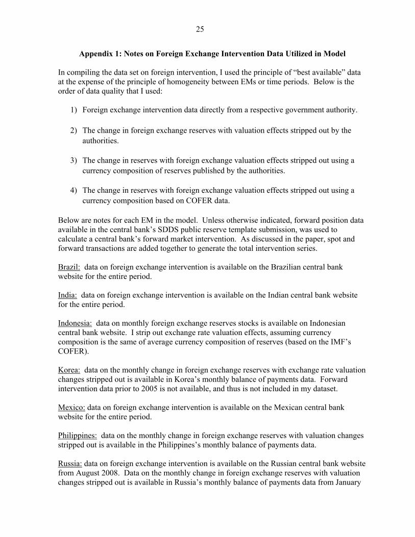
Appendix 1: Notes on Foreign Exchange Intervention Data Utilized in Model In compiling the data set on foreign intervention, I used the principle of “best available” data at the expense of the principle of homogeneity between EMs or time periods. Below is the order of data quality that I used:

1) Foreign exchange intervention data directly from a respective government authority.

2) The change in foreign exchange reserves with valuation effects stripped out by the authorities.

3) The change in reserves with foreign exchange valuation effects stripped out using a currency composition of reserves published by the authorities.

4) The change in reserves with foreign exchange valuation effects stripped out using a currency composition based on COFER data.

Below are notes for each EM in the model. Unless otherwise indicated, forward position data available in the central bank’s SDDS public reserve template submission, was used to calculate a central bank’s forward market intervention. As discussed in the paper, spot and forward transactions are added together to generate the total intervention series. Brazil: data on foreign exchange intervention is available on the Brazilian central bank website for the entire period. India: data on foreign exchange intervention is available on the Indian central bank website for the entire period. Indonesia: data on monthly foreign exchange reserves stocks is available on Indonesian central bank website. I strip out exchange rate valuation effects, assuming currency composition is the same of average currency composition of reserves (based on the IMF’s COFER). Korea: data on the monthly change in foreign exchange reserves with exchange rate valuation changes stripped out is available in Korea’s monthly balance of payments data. Forward intervention data prior to 2005 is not available, and thus is not included in my dataset. Mexico: data on foreign exchange intervention is available on the Mexican central bank website for the entire period. Philippines: data on the monthly change in foreign exchange reserves with valuation changes stripped out is available in the Philippines’s monthly balance of payments data. Russia: data on foreign exchange intervention is available on the Russian central bank website from August 2008. Data on the monthly change in foreign exchange reserves with valuation changes stripped out is available in Russia’s monthly balance of payments data from January

26

2007 to July 2008. Prior to January 2007, I use data on monthly foreign exchange reserves stocks, and strip out exchange rate valuation changes based on the currency composition of reserves listed in the Russian central bank’s annual reports. Taiwan: data on the change of foreign exchange reserves with valuation changes stripped out is available on the central bank website until November 2003. Prior to this, I use data on monthly foreign exchange reserves stocks, and strip out exchange rate valuation changes based on the average currency composition of reserves (based on the IMF’s COFER). Taiwan does not submit a reserve template to the IMF, and thus I do not include any possible forward transactions that Taiwan’s central bank may conduct as part of my estimate of foreign exchange intervention. Thailand: data on the monthly change in foreign exchange reserves with exchange rate valuation changes stripped out is available in Korea’s monthly balance of payments data. Poland: data on the monthly change in foreign exchange reserves with exchange rate valuation changes stripped out is available in Poland’s monthly balance of payments data. Israel: data on foreign exchange intervention is available on the Israeli central bank website for the entire period. Turkey: data on foreign exchange intervention is available on the Turkish central bank website for the entire period. South Africa: data on monthly foreign exchange reserves stocks is available on the South African central bank website. I strip out exchange rate valuation changes based on the currency composition of reserves listed in the South African central bank’s annual reports. Colombia: data on foreign exchange intervention is available on the Colombian central bank website for the entire period. Peru: data on foreign exchange intervention is available on the Peruvian central bank website for the entire period.

27

References

Almekinders, Geert J. & Eijffinger, Sylvester C. W., 1996. "A friction model of daily Bundesbank and Federal Reserve intervention," Journal of Banking & Finance, Elsevier, vol. 20(8), pages 1365-1380, September. Bastourre, Diego, Jorge Carrera, and Javier Ibarlucia, 2009, “What is Driving Reserves Accumulation,” Review of International Economics, Vol. 17, pp. 861–77. Frenkel, Michael; Perdzioch, Christian; Stadtmann, Georg “Japanese and US Interventions in the Yen/US Dollar Market: Estimating the Monetary Authorities’ Reaction Functions” Quarterly Review of Economics and Finance, Vol. 45 (2005), pp. 680-698. Ghosh, Atish; Ostry, Jonathan; and Tsangarides, Charalambos. “Shifting motives: explaining the buildup in official reserves in emerging markets since the 1980s,” 2012, IMF Working Papers 12/34, International Monetary Fund Gustavo Adler & Camilo E Tovar Mora. "Foreign Exchange Intervention: A Shield Against Appreciation Winds?," 2011, IMF Working Papers 11/165, International Monetary Fund. IMF Staff Paper. “Assessing Reserve Adequacy” (2011) Kim, Suk-Joong & Sheen, Jeffrey, 2002. "The determinants of foreign exchange intervention by central banks: evidence from Australia," Journal of International Money and Finance, Elsevier, vol. 21(5), pages 619-649, October. Kim, Suk-Joong & Sheen, Jeffrey, 2004. "Central Bank Interventions in the Yen-Dollar Spot Market," Working Papers 4, University of Sydney, School of Economics. Loiseau-Aslanidi, Olga. 2011. “Determinants and Effectiveness of Foreign Exchange Market Intervention in Georgia,” Emerging Markets Finance and Trade, Volume 47, Number 4, July-August 2011, 75-95 Obstfeld, Maurice, Jay C. Shambaugh, and Alan M. Taylor. 2008. “Financial Stability, the Trilemma, and International Reserves.” NBER Working Paper no. 14217. Ostry, Jonathan; Ghosh, Atish; Chamon, Marcos; “Two Targets, Two Instruments: Monetary and Exchange Rate Policies in Emerging Market Economies,” IMF Staff Discussion Note, SDN 12/01 Ozlu, P and A. Prokhorov (2008). "Modeling Central Bank Intervention as a Threshold Regression: Evidence from Turkey," Journal of Economic and Social Research, 10, 1-23.