Embed Size (px)
Citation preview
Presentation of FreeFem++F. Hecht,
Laboratoire Jacques-Louis LionsUniversite Pierre et Marie Curie
Paris, France
with O. Pironneau, A. Le Hyaric
http://www.freefem.org mailto:[email protected]
LJLL, Paris, Dec. 2015. F. Hecht et al. 7th FreeFem++ days 2015 1 / 185
Outline
1 Introduction
2 Tools
3 Academic Examples
4 Numerics Tools
5 Schwarz method with overlap
6 Exercices
7 No Linear Problem
8 Technical Remark on freefem++
LJLL, Paris, Dec. 2015. F. Hecht et al. 7th FreeFem++ days 2015 2 / 185
Outline
1 Introduction
2 Tools
3 Academic Examples
4 Numerics Tools
5 Schwarz method with overlap
6 Exercices
7 No Linear Problem
8 Technical Remark on freefem++
LJLL, Paris, Dec. 2015. F. Hecht et al. 7th FreeFem++ days 2015 3 / 185
Introduction
FreeFem++ is a software to solve numerically partial differential equations (PDE) inIR2) and in IR3) with finite elements methods. We used a user language to set andcontrol the problem. The FreeFem++ language allows for a quick specification oflinear PDE’s, with the variational formulation of a linear steady state problem and theuser can write they own script to solve no linear problem and time depend problem.You can solve coupled problem or problem with moving domain or eigenvalue problem,do mesh adaptation , compute error indicator, etc ...
By the way, FreeFem++ is build to play with abstract linear, bilinear form on FiniteElement Space and interpolation operator.
FreeFem++ is a freeware and this run on Mac, Unix and Window architecture, inparallel with MPI.To try of cell phonehttps://www.ljll.math.upmc.fr/lehyaric/ffjs/15.8/ffjs.htm
LJLL, Paris, Dec. 2015. F. Hecht et al. 7th FreeFem++ days 2015 4 / 185
Outline
1 IntroductionHistoryThe main characteristicsThe Changes form 12/09 to 06/11Last ChangesBasementWeak form
LJLL, Paris, Dec. 2015. F. Hecht et al. 7th FreeFem++ days 2015 5 / 185
History
1987 MacFem/PCFem the old ones (O. Pironneau in Pascal) no free.
1992 FreeFem rewrite in C++ (P1,P0 one mesh ) O. Pironneau, D. Bernardi, F.Hecht , C. Prudhomme (mesh adaptation , bamg).
1996 FreeFem+ rewrite in C++ (P1,P0 more mesh) O. Pironneau, D. Bernardi, F.Hecht (algebra of fucntion).
1998 FreeFem++ rewrite with an other finite element kernel and an new language ;F. Hecht, O. Pironneau, K.Ohtsuka.
1999 FreeFem 3d (S. Del Pino) , a fist 3d version base on fictitious domaine method.
2008 FreeFem++ v3 use a new finite element kernel multidimensionnels: 1d,2d,3d...
2014 FreefEM++ v3.34 parallel version
LJLL, Paris, Dec. 2015. F. Hecht et al. 7th FreeFem++ days 2015 6 / 185
For who, for what!
For what
1 R&D
2 Academic Research ,
3 Teaching of FEM, PDE, Weak form and variational form
4 Algorithmes prototyping
5 Numerical experimentation
6 Scientific computing and Parallel computing
For who: the researcher, engineer, professor, student...
The mailing list mailto:[email protected] with 410 memberswith a flux of 5-20 messages per day.
More than 2000 true Users ( more than 1000 download / month)
LJLL, Paris, Dec. 2015. F. Hecht et al. 7th FreeFem++ days 2015 7 / 185
Outline
1 IntroductionHistoryThe main characteristicsThe Changes form 12/09 to 06/11Last ChangesBasementWeak form
LJLL, Paris, Dec. 2015. F. Hecht et al. 7th FreeFem++ days 2015 8 / 185
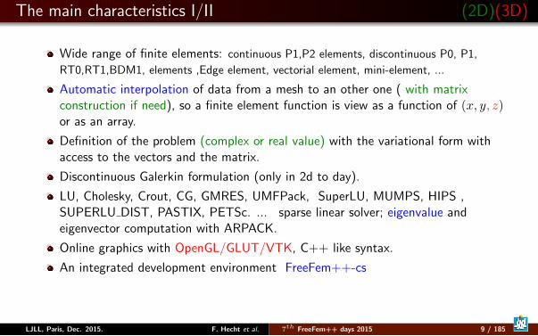
The main characteristics I/II (2D)(3D)
Wide range of finite elements: continuous P1,P2 elements, discontinuous P0, P1,
RT0,RT1,BDM1, elements ,Edge element, vectorial element, mini-element, ...
Automatic interpolation of data from a mesh to an other one ( with matrixconstruction if need), so a finite element function is view as a function of (x, y, z)or as an array.
Definition of the problem (complex or real value) with the variational form withaccess to the vectors and the matrix.
Discontinuous Galerkin formulation (only in 2d to day).
LU, Cholesky, Crout, CG, GMRES, UMFPack, SuperLU, MUMPS, HIPS ,SUPERLU DIST, PASTIX, PETSc. ... sparse linear solver; eigenvalue andeigenvector computation with ARPACK.
Online graphics with OpenGL/GLUT/VTK, C++ like syntax.
An integrated development environment FreeFem++-cs
LJLL, Paris, Dec. 2015. F. Hecht et al. 7th FreeFem++ days 2015 9 / 185

The main characteristics II/II (2D)(3D)
Analytic description of boundaries, with specification by the user of theintersection of boundaries in 2d.
Automatic mesh generator, based on the Delaunay-Voronoı algorithm. (2d,3d(tetgen) )
load and save Mesh, solution
Mesh adaptation based on metric, possibly anisotropic (only in 2d), with optionalautomatic computation of the metric from the Hessian of a solution. (2d,3d).
Link with other soft: parview, gmsh , vtk, medit, gnuplot
Dynamic linking to add plugin.
Full MPI interface
Nonlinear Optimisation tools: CG, Ipopt, NLOpt, stochastic
Wide range of examples: Navier-Stokes 3d, elasticity 3d, fluid structure, eigenvalue problem,
Schwarz’ domain decomposition algorithm, residual error indicator ...
LJLL, Paris, Dec. 2015. F. Hecht et al. 7th FreeFem++ days 2015 10 / 185
How to use
on Unix build a ”yours.edp” file with your favorite editor : emacs, vi, nedit, etc.EnterFreeFem++ yours.edp or FreeFem++ must be in a directoryof your PATH shell variable.
on Window, MacOs X build a ”yours.edp” file with your favorite text editor (raw text,not word text) : emacs, winedit, wordpad, bbedit, fraise ... and click onthe icon of the application FreeFem++ and load you file via de open filedialog box or drag and drop the icon of your built file on the applicationFreeFem++ icon.
LJLL, Paris, Dec. 2015. F. Hecht et al. 7th FreeFem++ days 2015 11 / 185
Outline
1 IntroductionHistoryThe main characteristicsThe Changes form 12/09 to 06/11Last ChangesBasementWeak form
LJLL, Paris, Dec. 2015. F. Hecht et al. 7th FreeFem++ days 2015 12 / 185
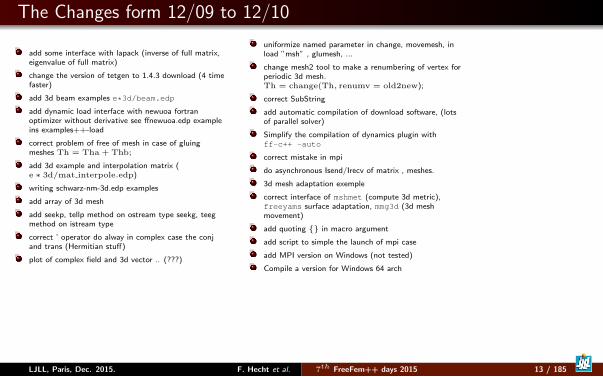
The Changes form 12/09 to 12/10
add some interface with lapack (inverse of full matrix,eigenvalue of full matrix)
change the version of tetgen to 1.4.3 download (4 timefaster)
add 3d beam examples e*3d/beam.edp
add dynamic load interface with newuoa fortranoptimizer without derivative see ffnewuoa.edp exampleins examples++-load
correct problem of free of mesh in case of gluingmeshes Th = Tha + Thb;
add 3d example and interpolation matrix (e ∗ 3d/mat interpole.edp)
writing schwarz-nm-3d.edp examples
add array of 3d mesh
add seekp, tellp method on ostream type seekg, teegmethod on istream type
correct ’ operator do alway in complex case the conjand trans (Hermitian stuff)
plot of complex field and 3d vector .. (???)
uniformize named parameter in change, movemesh, inload ”msh” , glumesh, ...
change mesh2 tool to make a renumbering of vertex forperiodic 3d mesh.Th = change(Th, renumv = old2new);
correct SubString
add automatic compilation of download software, (lotsof parallel solver)
Simplify the compilation of dynamics plugin withff-c++ -auto
correct mistake in mpi
do asynchronous Isend/Irecv of matrix , meshes.
3d mesh adaptation exemple
correct interface of mshmet (compute 3d metric),freeyams surface adaptation, mmg3d (3d meshmovement)
add quoting in macro argument
add script to simple the launch of mpi case
add MPI version on Windows (not tested)
Compile a version for Windows 64 arch
LJLL, Paris, Dec. 2015. F. Hecht et al. 7th FreeFem++ days 2015 13 / 185
Outline
1 IntroductionHistoryThe main characteristicsThe Changes form 12/09 to 06/11Last ChangesBasementWeak form
LJLL, Paris, Dec. 2015. F. Hecht et al. 7th FreeFem++ days 2015 14 / 185
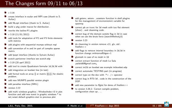
The Changes form 09/11 to 06/13
v 3.16
cmaes interface in scalar and MPI case (thank to S.Auliac)
add NLopt interface (thank to S. Auliac)
build a pkg under macos for distribution .
rewrite the isoline-P1 plugins
v 3.18 (11/01/2012)
add tools for adaptation of P2 and P3 finite elementswith metrics
add plugins with sequential mumps without mpi
add conversion of re and im part of complex sparsematrix
add Ipopt interface (thanks to Sylvain Auliac)
scotch partionner interface see scotch.edp
v 3.19 (20 april 2012)
add tool to create Quadrature formular 1d,2d,3d with
add integration on levelset line (in test)
add formal tools on array [] or matrix [[],[],] for elasiticproblem.
add new MUMPS parallel version plugin
add paradiso interface (MKL)
version 3.22
add multi windows graphics ; WindowIndex=0 in plotfunction and add new event in graphic windows * toset/unset default graphics stat to previous plot
add getenv, setenv , unsetenv function in shell pluginsfor the management of environnemnt variable foropenmp.
correct pb un trunc for 3d mesh with too flat element(sliver) , and cleanning code .
correct bug of the domain outsite flag in 3d in casewhen we use the brute force (searchMethod¿0)
version 3.23
do cleanning in version remove x11, glx, std :freefem++
add flags to remove internal boundary in 2d,3d infunction change rmInternalEdges=1
glumesh in case of no mesh in 2d
correct extract function of mesh Lo Sala¡[email protected]¿
correct int2d on levelset see example intlevelset.edp
correct automake TESTING part (in progress)
correct typo on the doc with .*= ./= operator
correct bug in RT0 3d , code in the construction of theDOF.
add new parameter to ffglut for demo of freefem++
to version 3.26-2. Correct compile problem,configuration clean up , ...
LJLL, Paris, Dec. 2015. F. Hecht et al. 7th FreeFem++ days 2015 15 / 185
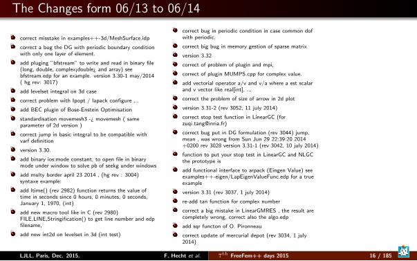
The Changes form 06/13 to 06/14
correct misstake in examples++-3d/MeshSurface.idp
correct a bug the DG with periodic boundary conditionwith only one layer of element.
add pluging ”bfstream” to write and read in binary file(long, double, complex¡double¿ and array) seebfstream.edp for an example. version 3.30-1 may/2014( hg rev: 3017)
add levelset integral on 3d case
correct problem with Ipopt / lapack configure ...
add BEC plugin of Bose-Enstein Optimisation
standardisation movemesh3 -¿ movemesh ( sameparameter of 2d version )
correct jump in basic integral to be compatible withvarf definition
version 3.30.
add binary ios:mode constant, to open file in binarymode under window to solve pb of seekg under windows
add multy border april 23 2014 , (hg rev : 3004)syntaxe example:
add ltime() (rev 2982) function returns the value oftime in seconds since 0 hours, 0 minutes, 0 seconds,January 1, 1970, (int)
add new macro tool like in C (rev 2980)FILE,LINE,Stringification() to get line number and edpfilename,
add new int2d on levelset in 3d (int test)
correct bug in periodic condition in case common dofwith periodic.
correct big bug in memory gestion of sparse matrix
version 3.32
correct of problem of plugin and mpi,
correct of plugin MUMPS.cpp for complex value.
add vectorial operator a/v and v/a where a est scalarand v vector like real[int], ...
correct the problem of size of arrow in 2d plot
version 3.31-2 (rev 3052, 11 july 2014)
correct stop test function in LinearGC ([email protected])
correct bug put in DG formulation (rev 3044) jump,mean , was wrong from Sun Jun 29 22:39:20 2014+0200 rev 3028 version 3.31-1 (rev 3042, 10 july 2014)
function to put your stop test in LinearGC and NLGCthe prototype is
add functional interface to arpack (Eingen Value) seeexamples++-eigen/LapEigenValueFunc.edp for a trueexample
version 3.31 (rev 3037, 1 july 2014)
re-add tan function for complex number
correct a big mistake in LinearGMRES , the result arecompletely wrong, correct also the algo.edp
add sqr functon of O. Pironneau
correct update of mercurial depot (rev 3034, 1 july2014)
LJLL, Paris, Dec. 2015. F. Hecht et al. 7th FreeFem++ days 2015 16 / 185
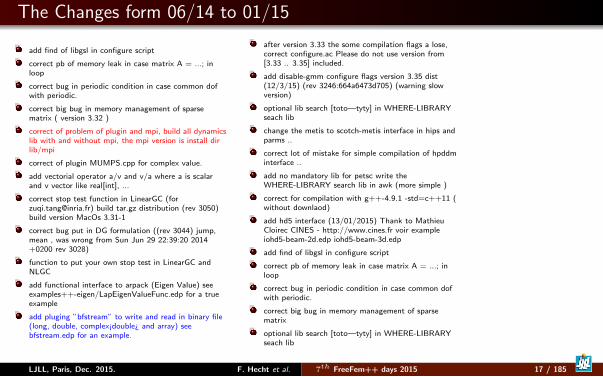
The Changes form 06/14 to 01/15
add find of libgsl in configure script
correct pb of memory leak in case matrix A = ...; inloop
correct bug in periodic condition in case common dofwith periodic.
correct big bug in memory management of sparsematrix ( version 3.32 )
correct of problem of plugin and mpi, build all dynamicslib with and without mpi, the mpi version is install dirlib/mpi
correct of plugin MUMPS.cpp for complex value.
add vectorial operator a/v and v/a where a is scalarand v vector like real[int], ...
correct stop test function in LinearGC ([email protected]) build tar.gz distribution (rev 3050)build version MacOs 3.31-1
correct bug put in DG formulation ((rev 3044) jump,mean , was wrong from Sun Jun 29 22:39:20 2014+0200 rev 3028)
function to put your own stop test in LinearGC andNLGC
add functional interface to arpack (Eigen Value) seeexamples++-eigen/LapEigenValueFunc.edp for a trueexample
add pluging ”bfstream” to write and read in binary file(long, double, complex¡double¿ and array) seebfstream.edp for an example.
after version 3.33 the some compilation flags a lose,correct configure.ac Please do not use version from[3.33 .. 3.35] included.
add disable-gmm configure flags version 3.35 dist(12/3/15) (rev 3246:664a6473d705) (warning slowversion)
optional lib search [toto—tyty] in WHERE-LIBRARYseach lib
change the metis to scotch-metis interface in hips andparms ..
correct lot of mistake for simple compilation of hpddminterface ..
add no mandatory lib for petsc write theWHERE-LIBRARY search lib in awk (more simple )
correct for compilation with g++-4.9.1 -std=c++11 (without downlaod)
add hd5 interface (13/01/2015) Thank to MathieuCloirec CINES - http://www.cines.fr voir exampleiohd5-beam-2d.edp iohd5-beam-3d.edp
add find of libgsl in configure script
correct pb of memory leak in case matrix A = ...; inloop
correct bug in periodic condition in case common dofwith periodic.
correct big bug in memory management of sparsematrix
optional lib search [toto—tyty] in WHERE-LIBRARYseach lib
LJLL, Paris, Dec. 2015. F. Hecht et al. 7th FreeFem++ days 2015 17 / 185
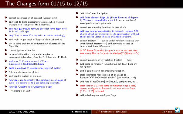
The Changes form 01/15 to 12/15
correct optimisation of convect (version 3.42 )
add tool do build quadrature formule when we splittriangle in 3 triangle for HCT element.
add new quadrature formula 3d exact form degre 6 to14 in qf11to25.cpp
map&key to know if a key exist in a map int[string], ....
add tools to get mesh of fespace Vh in 2d and 3d
try to solve problem of compatibility of petsc lib andff++ lib
correct hpddm examples
move of all hpddm code and examples inexamples++-hpddm ( Own by P. Jolivet and F. Hecht)
add new C1 Finite element HCT seeexamples++-load/bilabHCT.edp
build a windows 64 version under msys64 system
Add use ArrowSize= of size
add hppdm explain in the doc.
function cube to simplify the construction of mesh ofcube (like square in 2d ) see cube.edp example.
function ClosePoint in ClosePoint plugin
+= example of varf
add splitComm for hpddm
add finite element Edge13d (Finite Element of degrees1) Thanks to [email protected] and exemples ofwave guide in waveguide.edp
correct renumbering function in case of rhs
add new type of optimisation in integral, (version 3.3825june 2015) optimized=2 =¿ do optimisation withoutcheck can be usefull in case of random problem.
correct freefem++ launch under windows (remove waitwhen launch freefem++) and add wait in case oflaunch with launchff++.exe
in DG linear form with jump or mean in test fonctionwas wrong like varf a(u,v)=intalledges(Th)(jump(v)*u);
correct problem of try/catch in freefem++ func
add tools to remove/ renumbering dof (now build in)for hpddm
add a parameter in renumbering function.
clean examples-mpi, remove of all usage toRemoveDOF, bb2d bb3d, findDiff (see version 3.36)
add read of real[int,int], int[int,int], complex[int,int] ..
after version 3.33 the some compilation flags a lose,correct configure.ac Please do not use version from[3.33 .. 3.35] included.
add –disable-gmm configure flags
LJLL, Paris, Dec. 2015. F. Hecht et al. 7th FreeFem++ days 2015 18 / 185
Outline
1 IntroductionHistoryThe main characteristicsThe Changes form 12/09 to 06/11Last ChangesBasementWeak form
LJLL, Paris, Dec. 2015. F. Hecht et al. 7th FreeFem++ days 2015 19 / 185
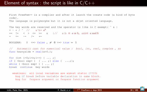
Element of syntax : the script is like in C/C++
First FreeFem++ is a complier and after it launch the create code (a kind of bytecode).The language is polymorphe but it is not a objet oriented language.
The key words are reserved and the operator is like in C exempt: ˆ & |+ - * / ˆ // aˆb= ab
== != < > <= >= & |// a|b ≡ a or b, a&b≡ a and b= += -= /= *=
BOOLEAN: 0 <=> false , 6= 0 <=> true = 1
// Automatic cast for numerical value : bool, int, reel, complex , sofunc heavyside = real(x>0.);
for (int i=0;i<n;i++) ... ;if ( <bool exp> ) ... ; else ...;;while ( <bool exp> ) ... ;break continue key words
weakless: all local variables are almost static (????)bug if break before variable declaration in same block.bug for fespace argument or fespace function argument
LJLL, Paris, Dec. 2015. F. Hecht et al. 7th FreeFem++ days 2015 20 / 185
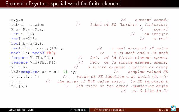
Element of syntax: special word for finite element
x,y,z // current coord.label, region // label of BC (border) , (interior)N.x, N.y, N.z, // normalint i = 0; // an integerreal a=2.5; // a reelbool b=(a<3.);real[int] array(10) ; // a real array of 10 valuemesh Th; mesh3 Th3; // a 2d mesh and a 3d meshfespace Vh(Th,P2); // Def. of 2d finite element space;fespace Vh3(Th3,P1); // Def. of 3d finite element space;Vh u=x; // a finite element function or arrayVh3<complex> uc = x+ 1i *y; // complex valued FEu(.5,.6,.7); // value of FE function u at point (.5, .6, .7)u[]; // the array of DoF value assoc. to FE function uu[][5]; // 6th value of the array (numbering begin
// at 0 like in C)
LJLL, Paris, Dec. 2015. F. Hecht et al. 7th FreeFem++ days 2015 21 / 185
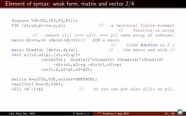
Element of syntax: weak form, matrix and vector 2/4
fespace V3h(Th,[P2,P2,P1]);V3h [u1,u2,p]=[x,y,z]; // a vectorial finite element
// function or array// remark u1[] <==> u2[] <==> p[] same array of unknown.
macro div(u,v) (dx(u)+dy(v))// EOM a macro// (like #define in C )
macro Grad(u) [dx(u),dy(u)] // the macro end with //varf a([u1,u2,p],[v1,v2,q])=
int2d(Th)( Grad(u1)’*Grad(v1) +Grad(u2)’*Grad(v2)-div(u1,u2)*q -div(v1,v2)*p)
+on(1,2,u1=g1,u2=g2);
matrix A=a(V3h,V3h,solver=UMFPACK);real[int] b=a(0,V3h);u2[] =Aˆ-1*b; // or you can put also u1[]= or p[].
LJLL, Paris, Dec. 2015. F. Hecht et al. 7th FreeFem++ days 2015 22 / 185
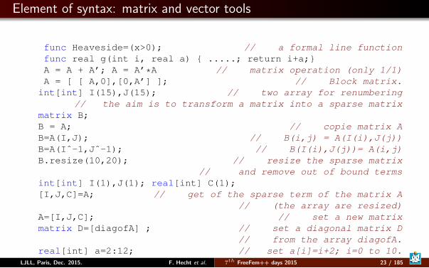
Element of syntax: matrix and vector tools
func Heaveside=(x>0); // a formal line functionfunc real g(int i, real a) .....; return i+a;A = A + A’; A = A’*A // matrix operation (only 1/1)A = [ [ A,0],[0,A’] ]; // Block matrix.int[int] I(15),J(15); // two array for renumbering
// the aim is to transform a matrix into a sparse matrixmatrix B;B = A; // copie matrix AB=A(I,J); // B(i,j) = A(I(i),J(j))B=A(Iˆ-1,Jˆ-1); // B(I(i),J(j))= A(i,j)B.resize(10,20); // resize the sparse matrix
// and remove out of bound termsint[int] I(1),J(1); real[int] C(1);[I,J,C]=A; // get of the sparse term of the matrix A
// (the array are resized)A=[I,J,C]; // set a new matrixmatrix D=[diagofA] ; // set a diagonal matrix D
// from the array diagofA.real[int] a=2:12; // set a[i]=i+2; i=0 to 10.
LJLL, Paris, Dec. 2015. F. Hecht et al. 7th FreeFem++ days 2015 23 / 185
Element of syntax formal computation on array
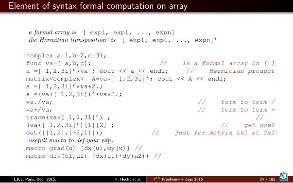
a formal array is [ exp1, exp1, ..., expn]the Hermitian transposition is [ exp1, exp1, ..., expn]’
complex a=1,b=2,c=3i;func va=[ a,b,c]; // is a formal array in [ ]a =[ 1,2,3i]’*va ; cout << a << endl; // Hermitian productmatrix<complex> A=va*[ 1,2,3i]’; cout << A << endl;a =[ 1,2,3i]’*va*2.;a =(va+[ 1,2,3i])’*va*2.;va./va; // term to term /va*/va; // term to term *trace(va*[ 1,2,3i]’) ; //(va*[ 1,2,3i]’)[1][2] ; // get coefdet([[1,2],[-2,1]]); // just for matrix 1x1 et 2x2usefull macro to def your edp.macro grad(u) [dx(u),dy(u)] //macro div(u1,u2) (dx(u1)+dy(u2)) //
LJLL, Paris, Dec. 2015. F. Hecht et al. 7th FreeFem++ days 2015 24 / 185
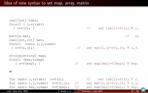
Idea of new syntax to set map, array, matrix
real[int] tab1;forall ( i,v;tab1)
v=f(i); // set tab[i]=f(i); ∀ i.
matrix mat; // orreal[int,int] mat;forall (auto i,j,v;mat) v=f(i,j); // set mat(i,j)=f(i,j); ∀ i,j.
string[string] map;forall (key,v;map)
v=f(key); // set map[key]=f(key); ∀ key.
or
for (auto i,v;tab1) v=f(i); // set tab[i]=f(i); ∀ i.for (auto i,j,v;mat) v=f(i,j); // set mat(i,j)=f(i,j); ∀ i,j.for (auto key,v;map) v=f(key); // set map[key]=f(key); ∀ key.
LJLL, Paris, Dec. 2015. F. Hecht et al. 7th FreeFem++ days 2015 25 / 185
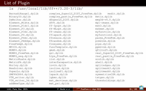
List of Pluginls /usr/local/lib/ff++/3.20-3/lib/
BernadiRaugel.dylib complex_SuperLU_DIST_FreeFem.dylib medit.dylibBinaryIO.dylib complex_pastix_FreeFem.dylib metis.dylibDxWriter.dylib dSuperLU_DIST.dylib mmg3d-v4.0.dylibElement_Mixte.dylib dfft.dylib mpi-cmaes.dylibElement_P1dc1.dylib ff-Ipopt.dylib msh3.dylibElement_P3.dylib ff-NLopt.dylib mshmet.dylibElement_P3dc.dylib ff-cmaes.dylib myfunction.dylibElement_P4.dylib fflapack.dylib myfunction2.dylibElement_P4dc.dylib ffnewuoa.dylib parms_FreeFem.dylibElement_PkEdge.dylib ffrandom.dylib pcm2rnm.dylibFreeFemQA.dylib freeyams.dylib pipe.dylibMPICG.dylib funcTemplate.dylib ppm2rnm.dylibMUMPS.dylib gmsh.dylib qf11to25.dylibMUMPS_FreeFem.dylib gsl.dylib real_SuperLU_DIST_FreeFem.dylibMUMPS_seq.dylib hips_FreeFem.dylib real_pastix_FreeFem.dylibMetricKuate.dylib ilut.dylib scotch.dylibMetricPk.dylib interfacepastix.dylib shell.dylibMorley.dylib iovtk.dylib splitedges.dylibNewSolver.dylib isoline.dylib splitmesh3.dylibSuperLu.dylib isolineP1.dylib splitmesh6.dylibUMFPACK64.dylib lapack.dylib symmetrizeCSR.dylibVTK_writer.dylib lgbmo.dylib tetgen.dylibVTK_writer_3d.dylib mat_dervieux.dylib thresholdings.dylibaddNewType.dylib mat_psi.dylib
LJLL, Paris, Dec. 2015. F. Hecht et al. 7th FreeFem++ days 2015 26 / 185
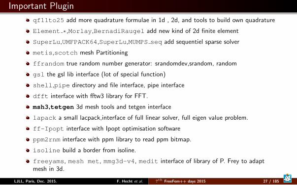
Important Plugin
qf11to25 add more quadrature formulae in 1d , 2d, and tools to build own quadrature
Element *,Morlay,BernadiRaugel add new kind of 2d finite element
SuperLu,UMFPACK64,SuperLu,MUMPS seq add sequentiel sparse solver
metis,scotch mesh Partitioning
ffrandom true random number generator: srandomdev,srandom, random
gsl the gsl lib interface (lot of special function)
shell,pipe directory and file interface, pipe interface
dfft interface with fftw3 library for FFT.
msh3,tetgen 3d mesh tools and tetgen interface
lapack a small lacpack,interface of full linear solver, full eigen value problem.
ff-Ipopt interface with Ipopt optimisation software
ppm2rnm interface with ppm library to read ppm bitmap.
isoline build a border from isoline.
freeyams, mesh met, mmg3d-v4, medit interface of library of P. Frey to adaptmesh in 3d.
LJLL, Paris, Dec. 2015. F. Hecht et al. 7th FreeFem++ days 2015 27 / 185
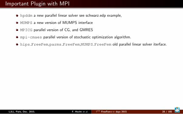
Important Plugin with MPI
hpddm a new parallel linear solver see schwarz.edp example,
MUMPS a new version of MUMPS interface
MPICG parallel version of CG, and GMRES
mpi-cmaes parallel version of stochastic optimization algorithm.
hips FreeFem,parms FreeFem,MUMPS FreeFem old parallel linear solver iterface.
LJLL, Paris, Dec. 2015. F. Hecht et al. 7th FreeFem++ days 2015 28 / 185
Outline
1 IntroductionHistoryThe main characteristicsThe Changes form 12/09 to 06/11Last ChangesBasementWeak form
LJLL, Paris, Dec. 2015. F. Hecht et al. 7th FreeFem++ days 2015 29 / 185
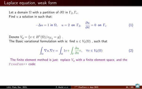
Laplace equation, weak form
Let a domain Ω with a partition of ∂Ω in Γ2,Γe.Find u a solution in such that:
−∆u = 1 in Ω, u = 2 on Γ2,∂u
∂~n= 0 on Γe (1)
Denote Vg = v ∈ H1(Ω)/v|Γ2= g .
The Basic variational formulation with is: find u ∈ V2(Ω) , such that∫Ω∇u.∇v =
∫Ω
1v+
∫Γ
∂u
∂nv, ∀v ∈ V0(Ω) (2)
The finite element method is just: replace Vg with a finite element space, and theFreeFem++ code:
LJLL, Paris, Dec. 2015. F. Hecht et al. 7th FreeFem++ days 2015 30 / 185
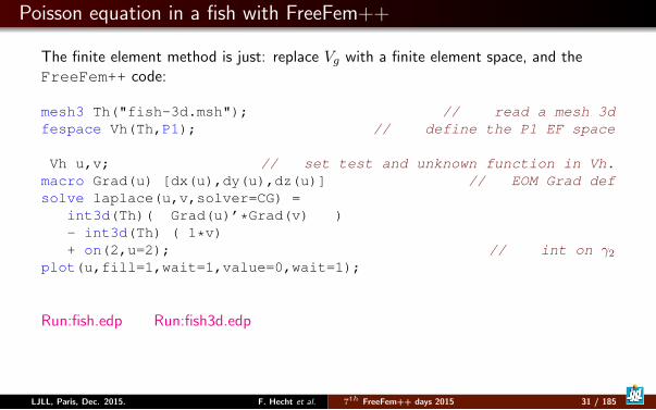
Poisson equation in a fish with FreeFem++
The finite element method is just: replace Vg with a finite element space, and theFreeFem++ code:
mesh3 Th("fish-3d.msh"); // read a mesh 3dfespace Vh(Th,P1); // define the P1 EF space
Vh u,v; // set test and unknown function in Vh.macro Grad(u) [dx(u),dy(u),dz(u)] // EOM Grad defsolve laplace(u,v,solver=CG) =
int3d(Th)( Grad(u)’*Grad(v) )- int3d(Th) ( 1*v)+ on(2,u=2); // int on γ2
plot(u,fill=1,wait=1,value=0,wait=1);
Run:fish.edp Run:fish3d.edp
LJLL, Paris, Dec. 2015. F. Hecht et al. 7th FreeFem++ days 2015 31 / 185
Important remark:on geometrical item label and region
All boundary (internal or nor) was define through a label number and this numberis define in the mesh data structure. The support of this label number is a edge in2d and a face in 3d and so FreeFem++ never use label on vertices.
To defined integration you can use the region (resp. label) number if you computeintegrate in domain (resp. boundary). They are no way to compute 1d integral in3d domain.
Today they are no Finite Element defined on surface.
You can put list of label or region in integer array (int[int]).
LJLL, Paris, Dec. 2015. F. Hecht et al. 7th FreeFem++ days 2015 32 / 185
Outline
1 Introduction
2 Tools
3 Academic Examples
4 Numerics Tools
5 Schwarz method with overlap
6 Exercices
7 No Linear Problem
8 Technical Remark on freefem++
LJLL, Paris, Dec. 2015. F. Hecht et al. 7th FreeFem++ days 2015 33 / 185
Outline
2 ToolsRemarks on weak form and boundary conditionsMesh generationBuild mesh from image3d meshMesh toolsAnisotropic Mesh adaptation
LJLL, Paris, Dec. 2015. F. Hecht et al. 7th FreeFem++ days 2015 34 / 185
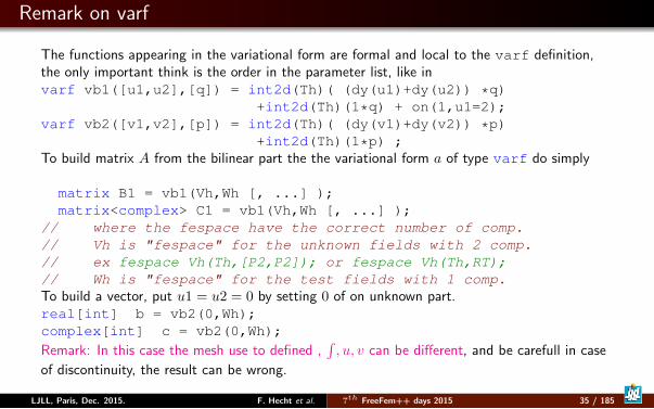
Remark on varf
The functions appearing in the variational form are formal and local to the varf definition,the only important think is the order in the parameter list, like invarf vb1([u1,u2],[q]) = int2d(Th)( (dy(u1)+dy(u2)) *q)
+int2d(Th)(1*q) + on(1,u1=2);varf vb2([v1,v2],[p]) = int2d(Th)( (dy(v1)+dy(v2)) *p)
+int2d(Th)(1*p) ;To build matrix A from the bilinear part the the variational form a of type varf do simply
matrix B1 = vb1(Vh,Wh [, ...] );matrix<complex> C1 = vb1(Vh,Wh [, ...] );
// where the fespace have the correct number of comp.// Vh is "fespace" for the unknown fields with 2 comp.// ex fespace Vh(Th,[P2,P2]); or fespace Vh(Th,RT);// Wh is "fespace" for the test fields with 1 comp.To build a vector, put u1 = u2 = 0 by setting 0 of on unknown part.real[int] b = vb2(0,Wh);complex[int] c = vb2(0,Wh);
Remark: In this case the mesh use to defined ,∫, u, v can be different, and be carefull in case
of discontinuity, the result can be wrong.
LJLL, Paris, Dec. 2015. F. Hecht et al. 7th FreeFem++ days 2015 35 / 185
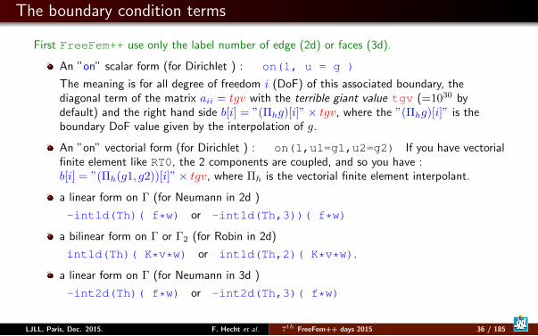
The boundary condition terms
First FreeFem++ use only the label number of edge (2d) or faces (3d).
An ”on” scalar form (for Dirichlet ) : on(1, u = g )
The meaning is for all degree of freedom i (DoF) of this associated boundary, thediagonal term of the matrix aii = tgv with the terrible giant value tgv (=1030 bydefault) and the right hand side b[i] = ”(Πhg)[i]”× tgv, where the ”(Πhg)[i]” is theboundary DoF value given by the interpolation of g.
An ”on” vectorial form (for Dirichlet ) : on(1,u1=g1,u2=g2) If you have vectorialfinite element like RT0, the 2 components are coupled, and so you have :b[i] = ”(Πh(g1, g2))[i]”× tgv, where Πh is the vectorial finite element interpolant.
a linear form on Γ (for Neumann in 2d )
-int1d(Th)( f*w) or -int1d(Th,3))( f*w)
a bilinear form on Γ or Γ2 (for Robin in 2d)
int1d(Th)( K*v*w) or int1d(Th,2)( K*v*w).
a linear form on Γ (for Neumann in 3d )
-int2d(Th)( f*w) or -int2d(Th,3)( f*w)
LJLL, Paris, Dec. 2015. F. Hecht et al. 7th FreeFem++ days 2015 36 / 185
Outline
2 ToolsRemarks on weak form and boundary conditionsMesh generationBuild mesh from image3d meshMesh toolsAnisotropic Mesh adaptation
LJLL, Paris, Dec. 2015. F. Hecht et al. 7th FreeFem++ days 2015 37 / 185
Build Mesh 2d
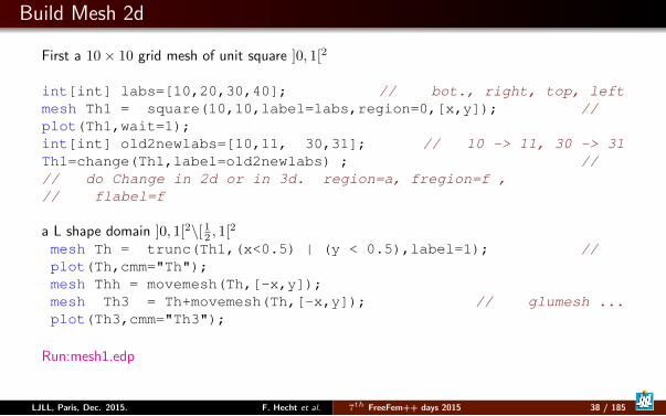
First a 10× 10 grid mesh of unit square ]0, 1[2
int[int] labs=[10,20,30,40]; // bot., right, top, leftmesh Th1 = square(10,10,label=labs,region=0,[x,y]); //plot(Th1,wait=1);int[int] old2newlabs=[10,11, 30,31]; // 10 -> 11, 30 -> 31Th1=change(Th1,label=old2newlabs) ; //// do Change in 2d or in 3d. region=a, fregion=f ,// flabel=f
a L shape domain ]0, 1[2\[ 12 , 1[2
mesh Th = trunc(Th1,(x<0.5) | (y < 0.5),label=1); //plot(Th,cmm="Th");mesh Thh = movemesh(Th,[-x,y]);mesh Th3 = Th+movemesh(Th,[-x,y]); // glumesh ...plot(Th3,cmm="Th3");
Run:mesh1.edp
LJLL, Paris, Dec. 2015. F. Hecht et al. 7th FreeFem++ days 2015 38 / 185
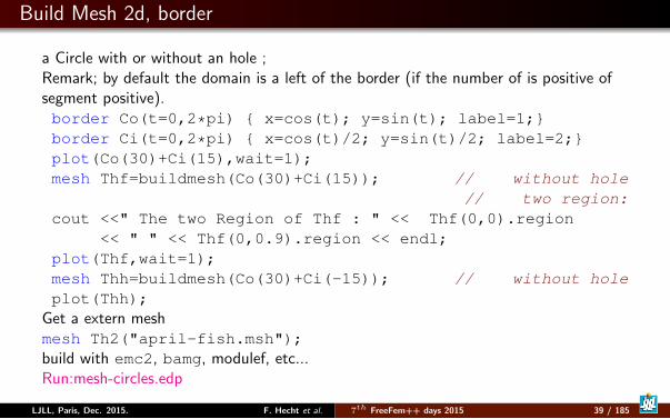
Build Mesh 2d, border
a Circle with or without an hole ;Remark; by default the domain is a left of the border (if the number of is positive ofsegment positive).border Co(t=0,2*pi) x=cos(t); y=sin(t); label=1;border Ci(t=0,2*pi) x=cos(t)/2; y=sin(t)/2; label=2;plot(Co(30)+Ci(15),wait=1);mesh Thf=buildmesh(Co(30)+Ci(15)); // without hole
// two region:cout <<" The two Region of Thf : " << Thf(0,0).region
<< " " << Thf(0,0.9).region << endl;plot(Thf,wait=1);mesh Thh=buildmesh(Co(30)+Ci(-15)); // without holeplot(Thh);
Get a extern meshmesh Th2("april-fish.msh");build with emc2, bamg, modulef, etc...Run:mesh-circles.edp
LJLL, Paris, Dec. 2015. F. Hecht et al. 7th FreeFem++ days 2015 39 / 185
Build Mesh 2d, more complicate with implicit loop
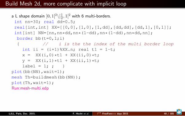
a L shape domain ]0, 1[2\[12 , 1[2 with 6 multi-borders.
int nn=30; real dd=0.5;real[int,int] XX=[[0,0],[1,0],[1,dd],[dd,dd],[dd,1],[0,1]];int[int] NN=[nn,nn*dd,nn*(1-dd),nn*(1-dd),nn*dd,nn];border bb(t=0,1;i) // i is the the index of the multi border loop
int ii = (i+1)%XX.n; real t1 = 1-t;x = XX(i,0)*t1 + XX(ii,0)*t;y = XX(i,1)*t1 + XX(ii,1)*t;label = 1; ;
plot(bb(NN),wait=1);mesh Th=buildmesh(bb(NN));plot(Th,wait=1);Run:mesh-multi.edp
LJLL, Paris, Dec. 2015. F. Hecht et al. 7th FreeFem++ days 2015 40 / 185
Outline
2 ToolsRemarks on weak form and boundary conditionsMesh generationBuild mesh from image3d meshMesh toolsAnisotropic Mesh adaptation
LJLL, Paris, Dec. 2015. F. Hecht et al. 7th FreeFem++ days 2015 41 / 185
Build mesh from image 1/2
load "ppm2rnm" load "isoline" load "shell"string lac="lac-oxford", lacjpg =lac+".jpg", lacpgm =lac+".pgm";if(stat(lacpgm)<0) exec("convert "+lacjpg+" "+lacpgm);real[int,int] Curves(3,1); int[int] be(1); int nc;
real[int,int] ff1(lacpgm); // read imageint nx = ff1.n, ny=ff1.m; // grey value in 0 to 1 (dark)mesh Th=square(nx-1,ny-1,[(nx-1)*(x),(ny-1)*(1-y)]);fespace Vh(Th,P1); Vh f1; f1[]=ff1; // array to fe function.real iso =0.3; // try some value to get correct isoreal[int] viso=[iso];nc=isoline(Th,f1,iso=iso,close=0,Curves,beginend=be,
smoothing=.1,ratio=0.5);for(int i=0; i<min(3,nc);++i) int i1=be(2*i),i2=be(2*i+1)-1;
plot(f1,viso=viso,[Curves(0,i1:i2),Curves(1,i1:i2)],wait=1,cmm=i);
LJLL, Paris, Dec. 2015. F. Hecht et al. 7th FreeFem++ days 2015 42 / 185
Build mesh from image 2/2
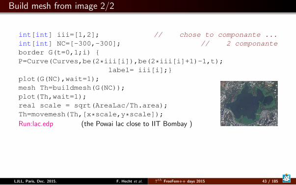
int[int] iii=[1,2]; // chose to componante ...int[int] NC=[-300,-300]; // 2 componanteborder G(t=0,1;i) P=Curve(Curves,be(2*iii[i]),be(2*iii[i]+1)-1,t);
label= iii[i];plot(G(NC),wait=1);mesh Th=buildmesh(G(NC));plot(Th,wait=1);real scale = sqrt(AreaLac/Th.area);Th=movemesh(Th,[x*scale,y*scale]);
Run:lac.edp (the Powai lac close to IIT Bombay )
LJLL, Paris, Dec. 2015. F. Hecht et al. 7th FreeFem++ days 2015 43 / 185
Outline
2 ToolsRemarks on weak form and boundary conditionsMesh generationBuild mesh from image3d meshMesh toolsAnisotropic Mesh adaptation
LJLL, Paris, Dec. 2015. F. Hecht et al. 7th FreeFem++ days 2015 44 / 185
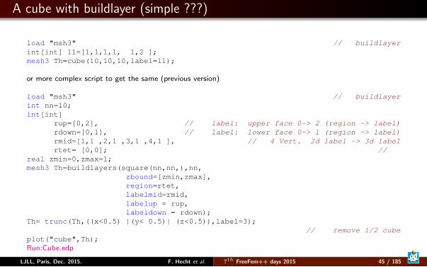
A cube with buildlayer (simple ???)
load "msh3" // buildlayerint[int] ll=[1,1,1,1, 1,2 ];mesh3 Th=cube(10,10,10,label=ll);
or more complex script to get the same (previous version)
load "msh3" // buildlayerint nn=10;int[int]
rup=[0,2], // label: upper face 0-> 2 (region -> label)rdown=[0,1], // label: lower face 0-> 1 (region -> label)rmid=[1,1 ,2,1 ,3,1 ,4,1 ], // 4 Vert. 2d label -> 3d labelrtet= [0,0]; //
real zmin=0,zmax=1;mesh3 Th=buildlayers(square(nn,nn,),nn,
zbound=[zmin,zmax],region=rtet,labelmid=rmid,labelup = rup,labeldown = rdown);
Th= trunc(Th,((x<0.5) |(y< 0.5)| (z<0.5)),label=3);// remove 1/2 cube
plot("cube",Th);Run:Cube.edp
LJLL, Paris, Dec. 2015. F. Hecht et al. 7th FreeFem++ days 2015 45 / 185
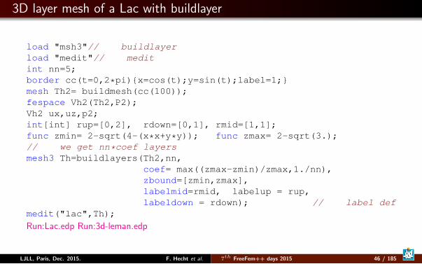
3D layer mesh of a Lac with buildlayer
load "msh3"// buildlayerload "medit"// meditint nn=5;border cc(t=0,2*pi)x=cos(t);y=sin(t);label=1;mesh Th2= buildmesh(cc(100));fespace Vh2(Th2,P2);Vh2 ux,uz,p2;int[int] rup=[0,2], rdown=[0,1], rmid=[1,1];func zmin= 2-sqrt(4-(x*x+y*y)); func zmax= 2-sqrt(3.);// we get nn*coef layersmesh3 Th=buildlayers(Th2,nn,
coef= max((zmax-zmin)/zmax,1./nn),zbound=[zmin,zmax],labelmid=rmid, labelup = rup,labeldown = rdown); // label def
medit("lac",Th);
Run:Lac.edp Run:3d-leman.edp
LJLL, Paris, Dec. 2015. F. Hecht et al. 7th FreeFem++ days 2015 46 / 185
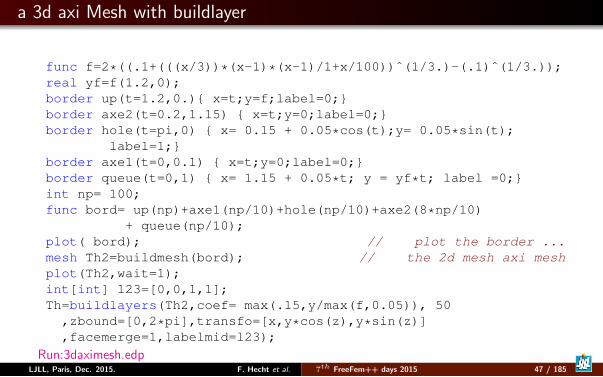
a 3d axi Mesh with buildlayer
func f=2*((.1+(((x/3))*(x-1)*(x-1)/1+x/100))ˆ(1/3.)-(.1)ˆ(1/3.));real yf=f(1.2,0);border up(t=1.2,0.) x=t;y=f;label=0;border axe2(t=0.2,1.15) x=t;y=0;label=0;border hole(t=pi,0) x= 0.15 + 0.05*cos(t);y= 0.05*sin(t);
label=1;border axe1(t=0,0.1) x=t;y=0;label=0;border queue(t=0,1) x= 1.15 + 0.05*t; y = yf*t; label =0;int np= 100;func bord= up(np)+axe1(np/10)+hole(np/10)+axe2(8*np/10)
+ queue(np/10);plot( bord); // plot the border ...mesh Th2=buildmesh(bord); // the 2d mesh axi meshplot(Th2,wait=1);int[int] l23=[0,0,1,1];Th=buildlayers(Th2,coef= max(.15,y/max(f,0.05)), 50
,zbound=[0,2*pi],transfo=[x,y*cos(z),y*sin(z)],facemerge=1,labelmid=l23);
Run:3daximesh.edpLJLL, Paris, Dec. 2015. F. Hecht et al. 7th FreeFem++ days 2015 47 / 185
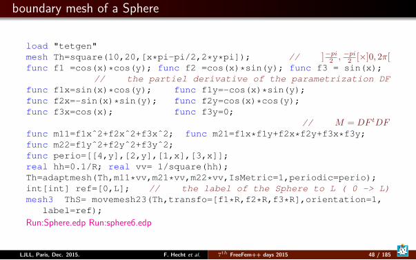
boundary mesh of a Sphere
load "tetgen"mesh Th=square(10,20,[x*pi-pi/2,2*y*pi]); // ]−pi2 , −pi2 [×]0, 2π[func f1 =cos(x)*cos(y); func f2 =cos(x)*sin(y); func f3 = sin(x);
// the partiel derivative of the parametrization DFfunc f1x=sin(x)*cos(y); func f1y=-cos(x)*sin(y);func f2x=-sin(x)*sin(y); func f2y=cos(x)*cos(y);func f3x=cos(x); func f3y=0;
// M = DF tDFfunc m11=f1xˆ2+f2xˆ2+f3xˆ2; func m21=f1x*f1y+f2x*f2y+f3x*f3y;func m22=f1yˆ2+f2yˆ2+f3yˆ2;func perio=[[4,y],[2,y],[1,x],[3,x]];real hh=0.1/R; real vv= 1/square(hh);Th=adaptmesh(Th,m11*vv,m21*vv,m22*vv,IsMetric=1,periodic=perio);int[int] ref=[0,L]; // the label of the Sphere to L ( 0 -> L)mesh3 ThS= movemesh23(Th,transfo=[f1*R,f2*R,f3*R],orientation=1,
label=ref);
Run:Sphere.edp Run:sphere6.edp
LJLL, Paris, Dec. 2015. F. Hecht et al. 7th FreeFem++ days 2015 48 / 185
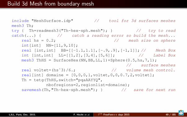
Build 3d Mesh from boundary mesh
include "MeshSurface.idp" // tool for 3d surfaces meshesmesh3 Th;try Th=readmesh3("Th-hex-sph.mesh"); // try to readcatch(...) // catch a reading error so build the mesh...
real hs = 0.2; // mesh size on sphereint[int] NN=[11,9,10];real [int,int] BB=[[-1.1,1.1],[-.9,.9],[-1,1]]; // Mesh Boxint [int,int] LL=[[1,2],[3,4],[5,6]]; // Label Boxmesh3 ThHS = SurfaceHex(NN,BB,LL,1)+Sphere(0.5,hs,7,1);
// surface meshesreal voltet=(hsˆ3)/6.; // volume mesh control.real[int] domaine = [0,0,0,1,voltet,0,0,0.7,2,voltet];Th = tetg(ThHS,switch="pqaAAYYQ",
nbofregions=2,regionlist=domaine);savemesh(Th,"Th-hex-sph.mesh"); // save for next run
LJLL, Paris, Dec. 2015. F. Hecht et al. 7th FreeFem++ days 2015 49 / 185
Outline
2 ToolsRemarks on weak form and boundary conditionsMesh generationBuild mesh from image3d meshMesh toolsAnisotropic Mesh adaptation
LJLL, Paris, Dec. 2015. F. Hecht et al. 7th FreeFem++ days 2015 50 / 185
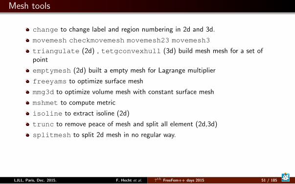
Mesh tools
change to change label and region numbering in 2d and 3d.
movemesh checkmovemesh movemesh23 movemesh3
triangulate (2d) , tetgconvexhull (3d) build mesh mesh for a set ofpoint
emptymesh (2d) built a empty mesh for Lagrange multiplier
freeyams to optimize surface mesh
mmg3d to optimize volume mesh with constant surface mesh
mshmet to compute metric
isoline to extract isoline (2d)
trunc to remove peace of mesh and split all element (2d,3d)
splitmesh to split 2d mesh in no regular way.
LJLL, Paris, Dec. 2015. F. Hecht et al. 7th FreeFem++ days 2015 51 / 185
Outline
2 ToolsRemarks on weak form and boundary conditionsMesh generationBuild mesh from image3d meshMesh toolsAnisotropic Mesh adaptation
LJLL, Paris, Dec. 2015. F. Hecht et al. 7th FreeFem++ days 2015 52 / 185
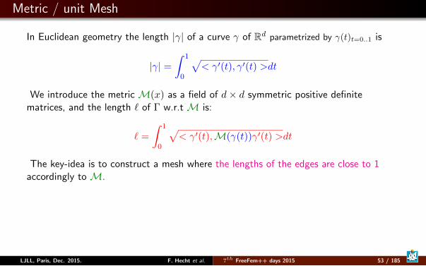
Metric / unit Mesh
In Euclidean geometry the length |γ| of a curve γ of Rd parametrized by γ(t)t=0..1 is
|γ| =∫ 1
0
√< γ′(t), γ′(t) >dt
We introduce the metric M(x) as a field of d× d symmetric positive definitematrices, and the length ` of Γ w.r.t M is:
` =
∫ 1
0
√< γ′(t),M(γ(t))γ′(t) >dt
The key-idea is to construct a mesh where the lengths of the edges are close to 1accordingly to M.
LJLL, Paris, Dec. 2015. F. Hecht et al. 7th FreeFem++ days 2015 53 / 185
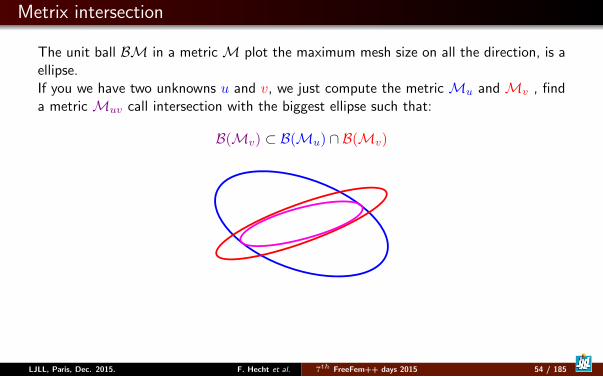
Metrix intersection
The unit ball BM in a metric M plot the maximum mesh size on all the direction, is aellipse.If you we have two unknowns u and v, we just compute the metric Mu and Mv , finda metric Muv call intersection with the biggest ellipse such that:
B(Mv) ⊂ B(Mu) ∩ B(Mv)
LJLL, Paris, Dec. 2015. F. Hecht et al. 7th FreeFem++ days 2015 54 / 185
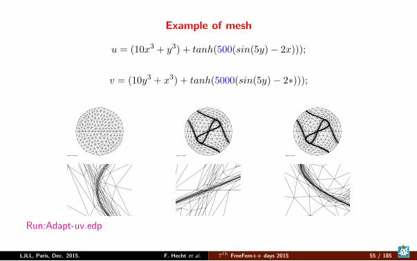
Example of mesh
u = (10x3 + y3) + tanh(500(sin(5y)− 2x)));
v = (10y3 + x3) + tanh(5000(sin(5y)− 2∗)));
Enter ? for help Enter ? for help Enter ? for help
Run:Adapt-uv.edp
LJLL, Paris, Dec. 2015. F. Hecht et al. 7th FreeFem++ days 2015 55 / 185
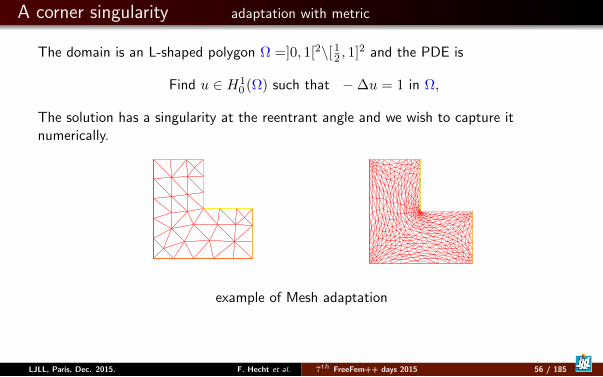
A corner singularity adaptation with metric
The domain is an L-shaped polygon Ω =]0, 1[2\[12 , 1]2 and the PDE is
Find u ∈ H10 (Ω) such that −∆u = 1 in Ω,
The solution has a singularity at the reentrant angle and we wish to capture itnumerically.
example of Mesh adaptation
LJLL, Paris, Dec. 2015. F. Hecht et al. 7th FreeFem++ days 2015 56 / 185
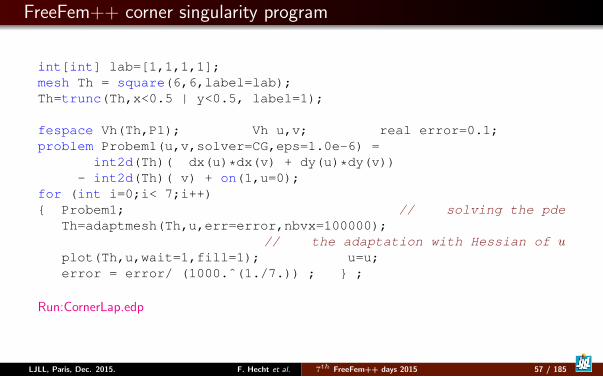
FreeFem++ corner singularity program
int[int] lab=[1,1,1,1];mesh Th = square(6,6,label=lab);Th=trunc(Th,x<0.5 | y<0.5, label=1);
fespace Vh(Th,P1); Vh u,v; real error=0.1;problem Probem1(u,v,solver=CG,eps=1.0e-6) =
int2d(Th)( dx(u)*dx(v) + dy(u)*dy(v))- int2d(Th)( v) + on(1,u=0);
for (int i=0;i< 7;i++) Probem1; // solving the pde
Th=adaptmesh(Th,u,err=error,nbvx=100000);// the adaptation with Hessian of u
plot(Th,u,wait=1,fill=1); u=u;error = error/ (1000.ˆ(1./7.)) ; ;
Run:CornerLap.edp
LJLL, Paris, Dec. 2015. F. Hecht et al. 7th FreeFem++ days 2015 57 / 185
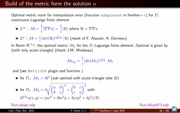
Build of the metric form the solution u
Optimal metric norm for interpolation error (function adaptmesh in freefem++) for P1
continuous Lagrange finite element
L∞ : M =1
ε|∇∇u| = 1
ε|H| where H = ∇∇u
Lp : M = 1ε |det(H)|
12p+2 |H| (result of F. Alauzet, A. Dervieux)
In Norm W 1,p, the optimal metric M` for the P` Lagrange finite element, Optimal is given by(with only acute triangle) (thank J-M. Mirebeau)
M`,p =1
ε(detM`)
1`p+2 M`
and (see MetricPk plugin and function )
for P1: M1 = H2 (sub optimal with acute triangle take H)
for P2: M2 = 3
√(a bb c
)2
+
(b cc a
)2
with
D(3)u(x, y) = (ax3 + 3bx2y + 3cxy2 + dy3)/3!,
Run:adapt.edp Run:AdaptP3.edp
LJLL, Paris, Dec. 2015. F. Hecht et al. 7th FreeFem++ days 2015 58 / 185
Outline
1 Introduction
2 Tools
3 Academic Examples
4 Numerics Tools
5 Schwarz method with overlap
6 Exercices
7 No Linear Problem
8 Technical Remark on freefem++
LJLL, Paris, Dec. 2015. F. Hecht et al. 7th FreeFem++ days 2015 59 / 185

Outline
3 Academic ExamplesLaplace/Poisson3d Poisson equation with mesh adaptationLinear elasticty equationStokes equationOptimize Time depend schema
LJLL, Paris, Dec. 2015. F. Hecht et al. 7th FreeFem++ days 2015 60 / 185
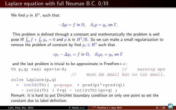
Laplace equation with full Neuman B.C. 0/III
We find p in H1, such that:
−∆p = f in Ω, ∂np = gn on Γ.
This problem is defined through a constant and mathematically the problem is wellpose iff
∫Ω f +
∫Γ gn = 0 and p is in H1/R. So we can make a small regularization to
remove the problem of constant by find pε ∈ H1 such that
εpε −∆pε = f in Ω, ∂npε = gn on Γ
and the last problem is trivial to be approximate in FreeFem++:Vh p,q; real eps=1e-8; // warning eps
// must be small but no too small.solve Laplace(p,q)= int2d(Th)( p*q*eps + grad(p)’*grad(q))
- int2d(Th) ( f*q) - int1d(Th)(gn*q) ;Remark: it is hard to put Dirichlet boundary condition on only one point so set theconstant due to label definition.
LJLL, Paris, Dec. 2015. F. Hecht et al. 7th FreeFem++ days 2015 61 / 185
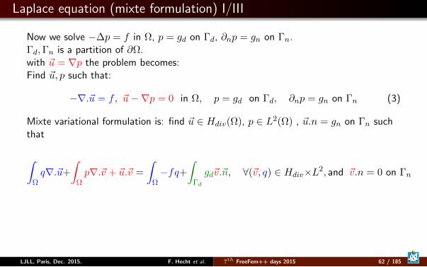
Laplace equation (mixte formulation) I/III
Now we solve −∆p = f in Ω, p = gd on Γd, ∂np = gn on Γn.Γd,Γn is a partition of ∂Ω.with ~u = ∇p the problem becomes:Find ~u, p such that:
−∇.~u = f, ~u−∇p = 0 in Ω, p = gd on Γd, ∂np = gn on Γn (3)
Mixte variational formulation is: find ~u ∈ Hdiv(Ω), p ∈ L2(Ω) , ~u.n = gn on Γn suchthat
∫Ωq∇.~u+
∫Ωp∇.~v + ~u.~v =
∫Ω−fq+
∫Γd
gd~v.~n, ∀(~v, q) ∈ Hdiv×L2, and ~v.n = 0 on Γn
LJLL, Paris, Dec. 2015. F. Hecht et al. 7th FreeFem++ days 2015 62 / 185
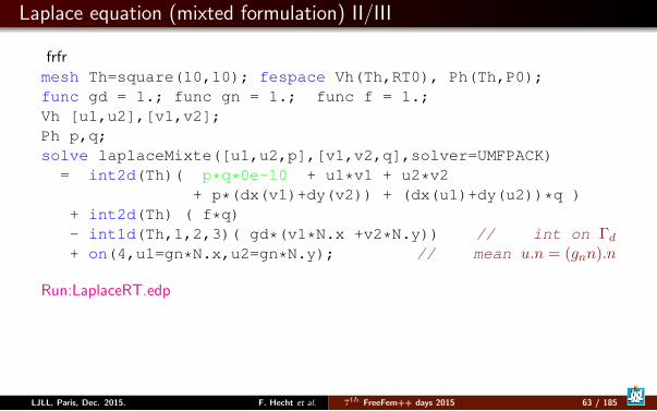
Laplace equation (mixted formulation) II/III
frfrmesh Th=square(10,10); fespace Vh(Th,RT0), Ph(Th,P0);func gd = 1.; func gn = 1.; func f = 1.;Vh [u1,u2],[v1,v2];Ph p,q;solve laplaceMixte([u1,u2,p],[v1,v2,q],solver=UMFPACK)= int2d(Th)( p*q*0e-10 + u1*v1 + u2*v2
+ p*(dx(v1)+dy(v2)) + (dx(u1)+dy(u2))*q )+ int2d(Th) ( f*q)- int1d(Th,1,2,3)( gd*(v1*N.x +v2*N.y)) // int on Γd+ on(4,u1=gn*N.x,u2=gn*N.y); // mean u.n = (gnn).n
Run:LaplaceRT.edp
LJLL, Paris, Dec. 2015. F. Hecht et al. 7th FreeFem++ days 2015 63 / 185
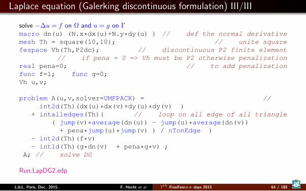
Laplace equation (Galerking discontinuous formulation) III/III
solve −∆u = f on Ω and u = g on Γmacro dn(u) (N.x*dx(u)+N.y*dy(u) ) // def the normal derivativemesh Th = square(10,10); // unite squarefespace Vh(Th,P2dc); // discontinuous P2 finite element
// if pena = 0 => Vh must be P2 otherwise penalizationreal pena=0; // to add penalizationfunc f=1; func g=0;Vh u,v;
problem A(u,v,solver=UMFPACK) = //int2d(Th)(dx(u)*dx(v)+dy(u)*dy(v) )
+ intalledges(Th)( // loop on all edge of all triangle( jump(v)*average(dn(u)) - jump(u)*average(dn(v))
+ pena*jump(u)*jump(v) ) / nTonEdge )- int2d(Th)(f*v)- int1d(Th)(g*dn(v) + pena*g*v) ;
A; // solve DG
Run:LapDG2.edp
LJLL, Paris, Dec. 2015. F. Hecht et al. 7th FreeFem++ days 2015 64 / 185
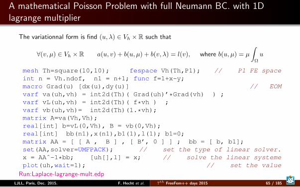
A mathematical Poisson Problem with full Neumann BC. with 1Dlagrange multiplier
The variationnal form is find (u, λ) ∈ Vh × R such that
∀(v, µ) ∈ Vh × R a(u, v) + b(u, µ) + b(v, λ) = l(v), where b(u, µ) = µ
∫Ω
u
mesh Th=square(10,10); fespace Vh(Th,P1); // P1 FE spaceint n = Vh.ndof, n1 = n+1; func f=1+x-y;macro Grad(u) [dx(u),dy(u)] // EOMvarf va(uh,vh) = int2d(Th)( Grad(uh)’*Grad(vh) ) ;varf vL(uh,vh) = int2d(Th)( f*vh ) ;varf vb(uh,vh)= int2d(Th)(1.*vh);matrix A=va(Vh,Vh);real[int] b=vL(0,Vh), B = vb(0,Vh);real[int] bb(n1),x(n1),b1(1),l(1); b1=0;matrix AA = [ [ A , B ] , [ B’, 0 ] ] ; bb = [ b, b1];set(AA,solver=UMFPACK); // set the type of linear solver.x = AAˆ-1*bb; [uh[],l] = x; // solve the linear systemeplot(uh,wait=1); // set the value
Run:Laplace-lagrange-mult.edp
LJLL, Paris, Dec. 2015. F. Hecht et al. 7th FreeFem++ days 2015 65 / 185

Outline
3 Academic ExamplesLaplace/Poisson3d Poisson equation with mesh adaptationLinear elasticty equationStokes equationOptimize Time depend schema
LJLL, Paris, Dec. 2015. F. Hecht et al. 7th FreeFem++ days 2015 66 / 185
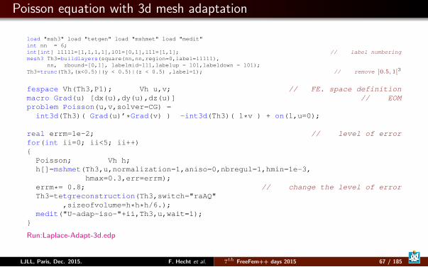
Poisson equation with 3d mesh adaptation
load "msh3" load "tetgen" load "mshmet" load "medit"int nn = 6;int[int] l1111=[1,1,1,1],l01=[0,1],l11=[1,1]; // label numberingmesh3 Th3=buildlayers(square(nn,nn,region=0,label=l1111),
nn, zbound=[0,1], labelmid=l11,labelup = l01,labeldown = l01);Th3=trunc(Th3,(x<0.5)|(y < 0.5)|(z < 0.5) ,label=1); // remove ]0.5, 1[3
fespace Vh(Th3,P1); Vh u,v; // FE. space definitionmacro Grad(u) [dx(u),dy(u),dz(u)] // EOMproblem Poisson(u,v,solver=CG) =
int3d(Th3)( Grad(u)’*Grad(v) ) -int3d(Th3)( 1*v ) + on(1,u=0);
real errm=1e-2; // level of errorfor(int ii=0; ii<5; ii++)
Poisson; Vh h;h[]=mshmet(Th3,u,normalization=1,aniso=0,nbregul=1,hmin=1e-3,
hmax=0.3,err=errm);errm*= 0.8; // change the level of errorTh3=tetgreconstruction(Th3,switch="raAQ"
,sizeofvolume=h*h*h/6.);medit("U-adap-iso-"+ii,Th3,u,wait=1);
Run:Laplace-Adapt-3d.edp
LJLL, Paris, Dec. 2015. F. Hecht et al. 7th FreeFem++ days 2015 67 / 185

Outline
3 Academic ExamplesLaplace/Poisson3d Poisson equation with mesh adaptationLinear elasticty equationStokes equationOptimize Time depend schema
LJLL, Paris, Dec. 2015. F. Hecht et al. 7th FreeFem++ days 2015 68 / 185
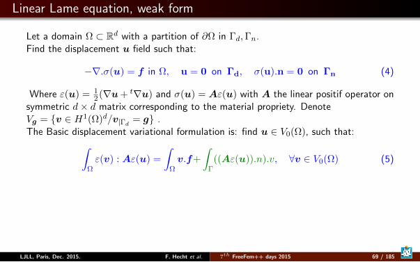
Linear Lame equation, weak form
Let a domain Ω ⊂ Rd with a partition of ∂Ω in Γd,Γn.Find the displacement u field such that:
−∇.σ(u) = f in Ω, u = 0 on Γd, σ(u).n = 0 on Γn (4)
Where ε(u) = 12(∇u+ t∇u) and σ(u) = Aε(u) with A the linear positif operator on
symmetric d× d matrix corresponding to the material propriety. DenoteVg = v ∈ H1(Ω)d/v|Γd
= g .The Basic displacement variational formulation is: find u ∈ V0(Ω), such that:∫
Ωε(v) : Aε(u) =
∫Ωv.f+
∫Γ((Aε(u)).n).v, ∀v ∈ V0(Ω) (5)
LJLL, Paris, Dec. 2015. F. Hecht et al. 7th FreeFem++ days 2015 69 / 185
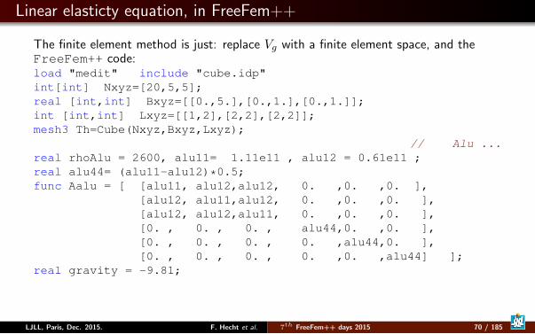
Linear elasticty equation, in FreeFem++
The finite element method is just: replace Vg with a finite element space, and theFreeFem++ code:load "medit" include "cube.idp"int[int] Nxyz=[20,5,5];real [int,int] Bxyz=[[0.,5.],[0.,1.],[0.,1.]];int [int,int] Lxyz=[[1,2],[2,2],[2,2]];mesh3 Th=Cube(Nxyz,Bxyz,Lxyz);
// Alu ...real rhoAlu = 2600, alu11= 1.11e11 , alu12 = 0.61e11 ;real alu44= (alu11-alu12)*0.5;func Aalu = [ [alu11, alu12,alu12, 0. ,0. ,0. ],
[alu12, alu11,alu12, 0. ,0. ,0. ],[alu12, alu12,alu11, 0. ,0. ,0. ],[0. , 0. , 0. , alu44,0. ,0. ],[0. , 0. , 0. , 0. ,alu44,0. ],[0. , 0. , 0. , 0. ,0. ,alu44] ];
real gravity = -9.81;
LJLL, Paris, Dec. 2015. F. Hecht et al. 7th FreeFem++ days 2015 70 / 185
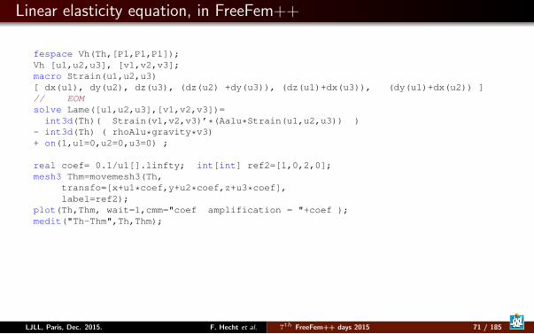
Linear elasticity equation, in FreeFem++
fespace Vh(Th,[P1,P1,P1]);Vh [u1,u2,u3], [v1,v2,v3];macro Strain(u1,u2,u3)[ dx(u1), dy(u2), dz(u3), (dz(u2) +dy(u3)), (dz(u1)+dx(u3)), (dy(u1)+dx(u2)) ]// EOMsolve Lame([u1,u2,u3],[v1,v2,v3])=
int3d(Th)( Strain(v1,v2,v3)’*(Aalu*Strain(u1,u2,u3)) )- int3d(Th) ( rhoAlu*gravity*v3)+ on(1,u1=0,u2=0,u3=0) ;
real coef= 0.1/u1[].linfty; int[int] ref2=[1,0,2,0];mesh3 Thm=movemesh3(Th,
transfo=[x+u1*coef,y+u2*coef,z+u3*coef],label=ref2);
plot(Th,Thm, wait=1,cmm="coef amplification = "+coef );medit("Th-Thm",Th,Thm);
LJLL, Paris, Dec. 2015. F. Hecht et al. 7th FreeFem++ days 2015 71 / 185
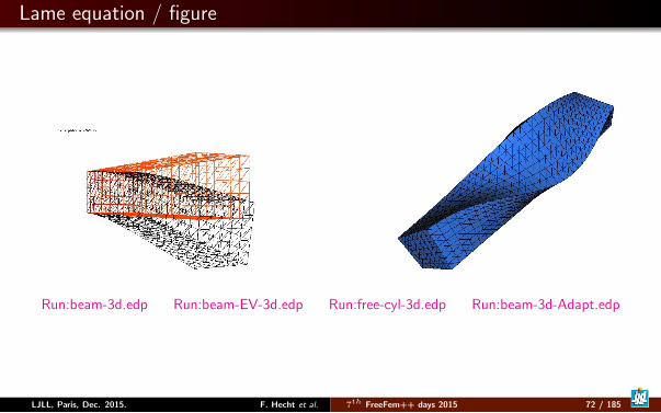
Lame equation / figure
Run:beam-3d.edp Run:beam-EV-3d.edp Run:free-cyl-3d.edp Run:beam-3d-Adapt.edp
LJLL, Paris, Dec. 2015. F. Hecht et al. 7th FreeFem++ days 2015 72 / 185
Outline
3 Academic ExamplesLaplace/Poisson3d Poisson equation with mesh adaptationLinear elasticty equationStokes equationOptimize Time depend schema
LJLL, Paris, Dec. 2015. F. Hecht et al. 7th FreeFem++ days 2015 73 / 185
Stokes equation
The Stokes equation is find a velocity field u = (u1, .., ud) and the pressure p ondomain Ω of Rd, such that
−∆u +∇p = 0 in Ω∇ · u = 0 in Ω
u = uΓ on Γ
where uΓ is a given velocity on boundary Γ.The classical variational formulation is: Find u ∈ H1(Ω)d with u|Γ = uΓ, andp ∈ L2(Ω)/R such that
∀v ∈ H10 (Ω)d, ∀q ∈ L2(Ω)/R,
∫Ω∇u : ∇v − p∇.v − q∇.u = 0
or now find p ∈ L2(Ω) such than (with ε = 10−10)
∀v ∈ H10 (Ω)d, ∀q ∈ L2(Ω),
∫Ω∇u : ∇v − p∇.v − q∇.u+ εpq = 0
LJLL, Paris, Dec. 2015. F. Hecht et al. 7th FreeFem++ days 2015 74 / 185
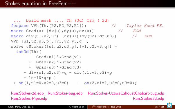
Stokes equation in FreeFem++
... build mesh .... Th (3d) T2d ( 2d)fespace VVh(Th,[P2,P2,P2,P1]); // Taylor Hood FE.macro Grad(u) [dx(u),dy(u),dz(u)] // EOMmacro div(u1,u2,u3) (dx(u1)+dy(u2)+dz(u3)) // EOMVVh [u1,u2,u3,p],[v1,v2,v3,q] ;solve vStokes([u1,u2,u3,p],[v1,v2,v3,q]) =int3d(Th)(
Grad(u1)’*Grad(v1)+ Grad(u2)’*Grad(v2)+ Grad(u3)’*Grad(v3)
- div(u1,u2,u3)*q - div(v1,v2,v3)*p- 1e-10*q*p )
+ on(1,u1=0,u2=0,u3=0) + on(2,u1=1,u2=0,u3=0);
Run:Stokes-2d.edp Run:Stokes-bug.edp Run:Stokes-UzawaCahouetChabart-bug.edpRun:Stokes-Pipe.edp Run:Stokes3d.edp
LJLL, Paris, Dec. 2015. F. Hecht et al. 7th FreeFem++ days 2015 75 / 185
Outline
3 Academic ExamplesLaplace/Poisson3d Poisson equation with mesh adaptationLinear elasticty equationStokes equationOptimize Time depend schema
LJLL, Paris, Dec. 2015. F. Hecht et al. 7th FreeFem++ days 2015 76 / 185
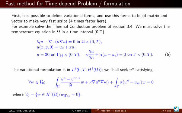
Fast method for Time depend Problem / formulation
First, it is possible to define variational forms, and use this forms to build matrix andvector to make very fast script (4 times faster here).For example solve the Thermal Conduction problem of section 3.4. We must solve thetemperature equation in Ω in a time interval (0,T).
∂tu−∇ · (κ∇u) = 0 in Ω× (0, T ),u(x, y, 0) = u0 + xu1
u = 30 on Γ24 × (0, T ), κ∂u
∂n+ α(u− ue) = 0 on Γ× (0, T ). (6)
The variational formulation is in L2(0, T ;H1(Ω)); we shall seek un satisfying
∀w ∈ V0;
∫Ω
un − un−1
δtw + κ∇un∇w) +
∫Γα(un − uue)w = 0
where V0 = w ∈ H1(Ω)/w|Γ24= 0.
LJLL, Paris, Dec. 2015. F. Hecht et al. 7th FreeFem++ days 2015 77 / 185
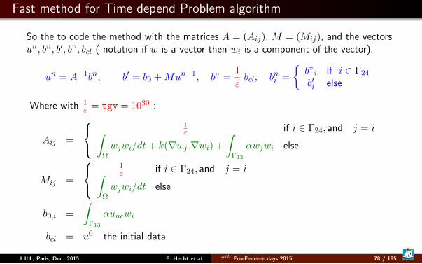
Fast method for Time depend Problem algorithm
So the to code the method with the matrices A = (Aij), M = (Mij), and the vectorsun, bn, b′, b”, bcl ( notation if w is a vector then wi is a component of the vector).
un = A−1bn, b′ = b0 +Mun−1, b” =1
εbcl, bni =
b”i if i ∈ Γ24
b′i else
Where with 1ε = tgv = 1030 :
Aij =
1ε if i ∈ Γ24, and j = i∫
Ωwjwi/dt+ k(∇wj .∇wi) +
∫Γ13
αwjwi else
Mij =
1ε if i ∈ Γ24, and j = i∫
Ωwjwi/dt else
b0,i =
∫Γ13
αuuewi
bcl = u0 the initial data
LJLL, Paris, Dec. 2015. F. Hecht et al. 7th FreeFem++ days 2015 78 / 185
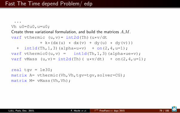
Fast The Time depend Problem/ edp
...Vh u0=fu0,u=u0;Create three variational formulation, and build the matrices A,M .varf vthermic (u,v)= int2d(Th)(u*v/dt
+ k*(dx(u) * dx(v) + dy(u) * dy(v)))+ int1d(Th,1,3)(alpha*u*v) + on(2,4,u=1);
varf vthermic0(u,v) = int1d(Th,1,3)(alpha*ue*v);varf vMass (u,v)= int2d(Th)( u*v/dt) + on(2,4,u=1);
real tgv = 1e30;matrix A= vthermic(Vh,Vh,tgv=tgv,solver=CG);matrix M= vMass(Vh,Vh);
LJLL, Paris, Dec. 2015. F. Hecht et al. 7th FreeFem++ days 2015 79 / 185
Fast The Time depend Problem/ edp
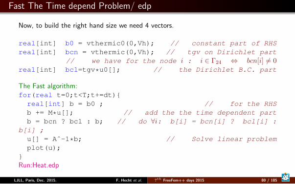
Now, to build the right hand size we need 4 vectors.
real[int] b0 = vthermic0(0,Vh); // constant part of RHSreal[int] bcn = vthermic(0,Vh); // tgv on Dirichlet part
// we have for the node i : i ∈ Γ24 ⇔ bcn[i] 6= 0real[int] bcl=tgv*u0[]; // the Dirichlet B.C. part
The Fast algorithm:for(real t=0;t<T;t+=dt)real[int] b = b0 ; // for the RHSb += M*u[]; // add the the time dependent partb = bcn ? bcl : b; // do ∀i: b[i] = bcn[i] ? bcl[i] :
b[i] ;u[] = Aˆ-1*b; // Solve linear problemplot(u);
Run:Heat.edp
LJLL, Paris, Dec. 2015. F. Hecht et al. 7th FreeFem++ days 2015 80 / 185
Outline
1 Introduction
2 Tools
3 Academic Examples
4 Numerics Tools
5 Schwarz method with overlap
6 Exercices
7 No Linear Problem
8 Technical Remark on freefem++
LJLL, Paris, Dec. 2015. F. Hecht et al. 7th FreeFem++ days 2015 81 / 185
Outline
4 Numerics ToolsConnectivityInput/OutputTricksEigenvalueOptimization ToolsMPI/Parallel
LJLL, Paris, Dec. 2015. F. Hecht et al. 7th FreeFem++ days 2015 82 / 185
Get Connectivity
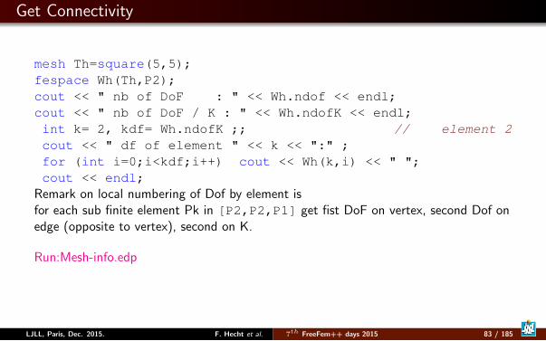
mesh Th=square(5,5);fespace Wh(Th,P2);cout << " nb of DoF : " << Wh.ndof << endl;cout << " nb of DoF / K : " << Wh.ndofK << endl;int k= 2, kdf= Wh.ndofK ;; // element 2cout << " df of element " << k << ":" ;for (int i=0;i<kdf;i++) cout << Wh(k,i) << " ";cout << endl;
Remark on local numbering of Dof by element isfor each sub finite element Pk in [P2,P2,P1] get fist DoF on vertex, second Dof onedge (opposite to vertex), second on K.
Run:Mesh-info.edp
LJLL, Paris, Dec. 2015. F. Hecht et al. 7th FreeFem++ days 2015 83 / 185
Outline
4 Numerics ToolsConnectivityInput/OutputTricksEigenvalueOptimization ToolsMPI/Parallel
LJLL, Paris, Dec. 2015. F. Hecht et al. 7th FreeFem++ days 2015 84 / 185
Save/Restore
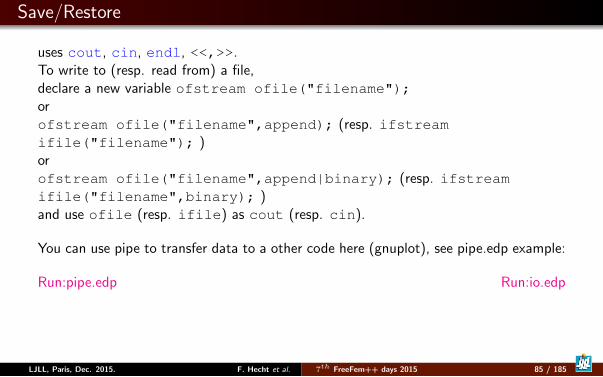
uses cout, cin, endl, <<,>>.To write to (resp. read from) a file,declare a new variable ofstream ofile("filename");orofstream ofile("filename",append); (resp. ifstreamifile("filename"); )orofstream ofile("filename",append|binary); (resp. ifstreamifile("filename",binary); )and use ofile (resp. ifile) as cout (resp. cin).
You can use pipe to transfer data to a other code here (gnuplot), see pipe.edp example:
Run:pipe.edp Run:io.edp
LJLL, Paris, Dec. 2015. F. Hecht et al. 7th FreeFem++ days 2015 85 / 185

Outline
4 Numerics ToolsConnectivityInput/OutputTricksEigenvalueOptimization ToolsMPI/Parallel
LJLL, Paris, Dec. 2015. F. Hecht et al. 7th FreeFem++ days 2015 86 / 185
Freefem++ Tricks
What is simple to do with freefem++ :
Evaluate variational form with Boundary condition or not.
Do interpolation
Do linear algebra
Solve sparse problem.
LJLL, Paris, Dec. 2015. F. Hecht et al. 7th FreeFem++ days 2015 87 / 185
Freefem++ Trick: extract Dof list of border
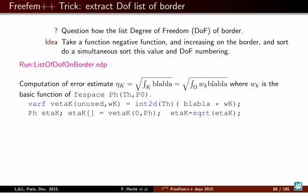
? Question how the list Degree of Freedom (DoF) of border.
Idea Take a function negative function, and increasing on the border, and sortdo a simultaneous sort this value and DoF numbering.
Run:ListOfDofOnBorder.edp
Computation of error estimate ηK =√∫
K blabla =√∫
Ωwkblabla where wk is the
basic function of fespace Ph(Th,P0).varf vetaK(unused,wK) = int2d(Th)( blabla * wK);Ph etaK; etaK[] = vetaK(0,Ph); etaK=sqrt(etaK);
LJLL, Paris, Dec. 2015. F. Hecht et al. 7th FreeFem++ days 2015 88 / 185
Freefem++ Tricks
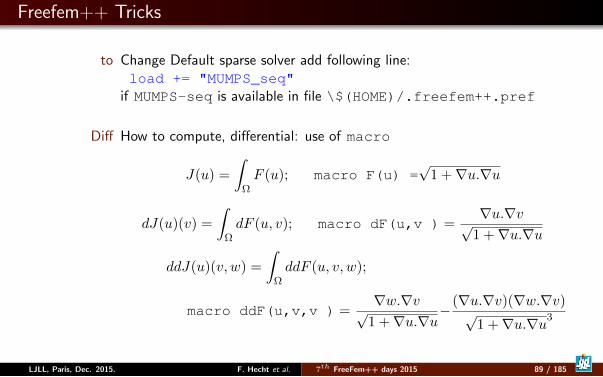
to Change Default sparse solver add following line:load += "MUMPS_seq"
if MUMPS-seq is available in file \$(HOME)/.freefem++.pref
Diff How to compute, differential: use of macro
J(u) =
∫ΩF (u); macro F(u) =
√1 +∇u.∇u
dJ(u)(v) =
∫ΩdF (u, v); macro dF(u,v ) =
∇u.∇v√1 +∇u.∇u
ddJ(u)(v, w) =
∫ΩddF (u, v, w);
macro ddF(u,v,v ) =∇w.∇v√
1 +∇u.∇u−(∇u.∇v)(∇w.∇v)√
1 +∇u.∇u3
LJLL, Paris, Dec. 2015. F. Hecht et al. 7th FreeFem++ days 2015 89 / 185
Outline
4 Numerics ToolsConnectivityInput/OutputTricksEigenvalueOptimization ToolsMPI/Parallel
LJLL, Paris, Dec. 2015. F. Hecht et al. 7th FreeFem++ days 2015 90 / 185
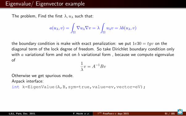
Eigenvalue/ Eigenvector example
The problem, Find the first λ, uλ such that:
a(uλ, v) =
∫Ω∇uλ∇v = λ
∫Ωuλv = λb(uλ, v)
the boundary condition is make with exact penalization: we put 1e30 = tgv on thediagonal term of the lock degree of freedom. So take Dirichlet boundary condition onlywith a variational form and not on b variational form , because we compute eigenvalueof
1
λv = A−1Bv
Otherwise we get spurious mode.Arpack interface:int k=EigenValue(A,B,sym=true,value=ev,vector=eV);
LJLL, Paris, Dec. 2015. F. Hecht et al. 7th FreeFem++ days 2015 91 / 185
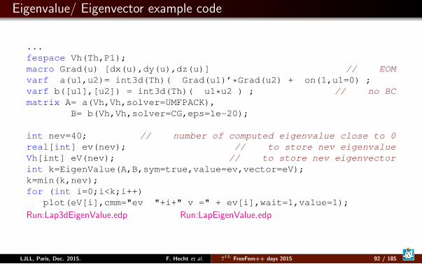
Eigenvalue/ Eigenvector example code
...fespace Vh(Th,P1);macro Grad(u) [dx(u),dy(u),dz(u)] // EOMvarf a(u1,u2)= int3d(Th)( Grad(u1)’*Grad(u2) + on(1,u1=0) ;varf b([u1],[u2]) = int3d(Th)( u1*u2 ) ; // no BCmatrix A= a(Vh,Vh,solver=UMFPACK),
B= b(Vh,Vh,solver=CG,eps=1e-20);
int nev=40; // number of computed eigenvalue close to 0real[int] ev(nev); // to store nev eigenvalueVh[int] eV(nev); // to store nev eigenvectorint k=EigenValue(A,B,sym=true,value=ev,vector=eV);k=min(k,nev);for (int i=0;i<k;i++)
plot(eV[i],cmm="ev "+i+" v =" + ev[i],wait=1,value=1);
Run:Lap3dEigenValue.edp Run:LapEigenValue.edp
LJLL, Paris, Dec. 2015. F. Hecht et al. 7th FreeFem++ days 2015 92 / 185
Outline
4 Numerics ToolsConnectivityInput/OutputTricksEigenvalueOptimization ToolsMPI/Parallel
LJLL, Paris, Dec. 2015. F. Hecht et al. 7th FreeFem++ days 2015 93 / 185
Ipopt optimizer
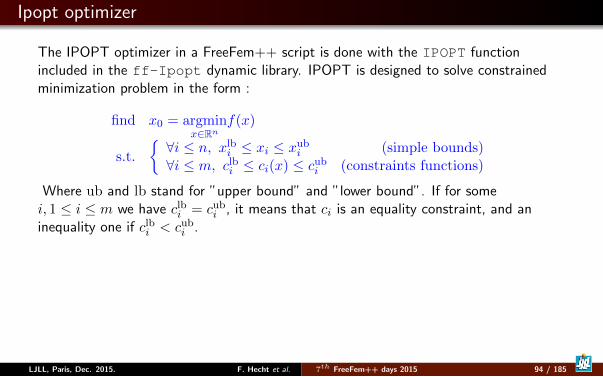
The IPOPT optimizer in a FreeFem++ script is done with the IPOPT functionincluded in the ff-Ipopt dynamic library. IPOPT is designed to solve constrainedminimization problem in the form :
find x0 = argminx∈Rn
f(x)
s.t.
∀i ≤ n, xlb
i ≤ xi ≤ xubi (simple bounds)
∀i ≤ m, clbi ≤ ci(x) ≤ cub
i (constraints functions)
Where ub and lb stand for ”upper bound” and ”lower bound”. If for somei, 1 ≤ i ≤ m we have clb
i = cubi , it means that ci is an equality constraint, and an
inequality one if clbi < cub
i .
LJLL, Paris, Dec. 2015. F. Hecht et al. 7th FreeFem++ days 2015 94 / 185
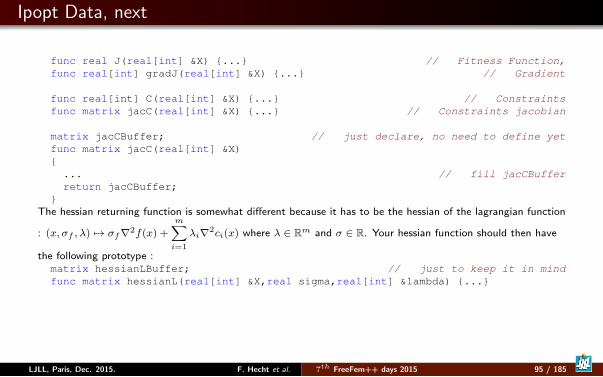
Ipopt Data, next
func real J(real[int] &X) ... // Fitness Function,func real[int] gradJ(real[int] &X) ... // Gradient
func real[int] C(real[int] &X) ... // Constraintsfunc matrix jacC(real[int] &X) ... // Constraints jacobian
matrix jacCBuffer; // just declare, no need to define yetfunc matrix jacC(real[int] &X)... // fill jacCBufferreturn jacCBuffer;
The hessian returning function is somewhat different because it has to be the hessian of the lagrangian function
: (x, σf , λ) 7→ σf∇2f(x) +m∑i=1
λi∇2ci(x) where λ ∈ Rm and σ ∈ R. Your hessian function should then have
the following prototype :matrix hessianLBuffer; // just to keep it in mindfunc matrix hessianL(real[int] &X,real sigma,real[int] &lambda) ...
LJLL, Paris, Dec. 2015. F. Hecht et al. 7th FreeFem++ days 2015 95 / 185
Ipopt Call
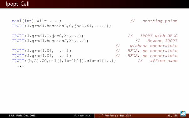
real[int] Xi = ... ; // starting pointIPOPT(J,gradJ,hessianL,C,jacC,Xi, ... );
IPOPT(J,gradJ,C,jacC,Xi,...); // IPOPT with BFGSIPOPT(J,gradJ,hessianJ,Xi,...); // Newton IPOPT
// without constraintsIPOPT(J,gradJ,Xi, ... ); // BFGS, no constraintsIPOPT(J,gradJ,Xi, ... ); // BFGS, no constraintsIPOPT([b,A],CC,ui1[],lb=lb1[],clb=cl[]..); // affine case
...
LJLL, Paris, Dec. 2015. F. Hecht et al. 7th FreeFem++ days 2015 96 / 185
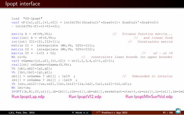
Ipopt interface
load "ff-Ipopt"varf vP([u1,u2],[v1,v2]) = int2d(Th)(Grad(u1)’*Grad(v1)+ Grad(u2)’*Grad(v2))- int2d(Th)(f1*v1+f2*v2);
matrix A = vP(Vh,Vh); // Fitness function matrix...real[int] b = vP(0,Vh); // and linear formint[int] II1=[0],II2=[1]; // Constraints matrixmatrix C1 = interpolate (Wh,Vh, U2Vc=II1);matrix C2 = interpolate (Wh,Vh, U2Vc=II2);matrix CC = -1*C1 + C2; // u2 - u1 >0Wh cl=0; // constraints lower bounds (no upper bounds)varf vGamma([u1,u2],[v1,v2]) = on(1,2,3,4,u1=1,u2=1);real[int] onGamma=vGamma(0,Vh);Vh [ub1,ub2]=[g1,g2];Vh [lb1,lb2]=[g1,g2];ub1[] = onGamma ? ub1[] : 1e19 ; // Unbounded in interiorlb1[] = onGamma ? lb1[] : -1e19 ;Vh [uzi,uzi2]=[uz,uz2],[lzi,lzi2]=[lz,lz2],[ui1,ui2]=[u1,u2];;Wh lmi=lm;IPOPT([b,A],CC,ui1[],lb=lb1[],clb=cl[],ub=ub1[],warmstart=iter>1,uz=uzi[],lz=lzi[],lm=lmi[]);
Run:IpoptLap.edp Run:IpoptVI2.edp Run:IpoptMinSurfVol.edp
LJLL, Paris, Dec. 2015. F. Hecht et al. 7th FreeFem++ days 2015 97 / 185
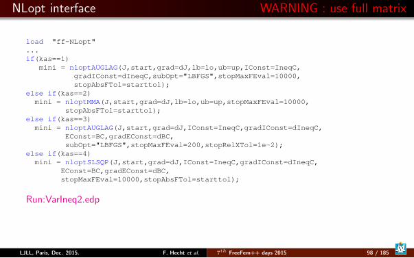
NLopt interface WARNING : use full matrix
load "ff-NLopt"...if(kas==1)
mini = nloptAUGLAG(J,start,grad=dJ,lb=lo,ub=up,IConst=IneqC,gradIConst=dIneqC,subOpt="LBFGS",stopMaxFEval=10000,stopAbsFTol=starttol);
else if(kas==2)mini = nloptMMA(J,start,grad=dJ,lb=lo,ub=up,stopMaxFEval=10000,
stopAbsFTol=starttol);else if(kas==3)
mini = nloptAUGLAG(J,start,grad=dJ,IConst=IneqC,gradIConst=dIneqC,EConst=BC,gradEConst=dBC,subOpt="LBFGS",stopMaxFEval=200,stopRelXTol=1e-2);
else if(kas==4)mini = nloptSLSQP(J,start,grad=dJ,IConst=IneqC,gradIConst=dIneqC,
EConst=BC,gradEConst=dBC,stopMaxFEval=10000,stopAbsFTol=starttol);
Run:VarIneq2.edp
LJLL, Paris, Dec. 2015. F. Hecht et al. 7th FreeFem++ days 2015 98 / 185
Stochastic interface
This algorithm works with a normal multivariate distribution in the parameters spaceand try to adapt its covariance matrix using the information provides by the successivefunction evaluations. Syntaxe: cmaes(J,u[],..) ( )From http://www.lri.fr/˜hansen/javadoc/fr/inria/optimization/cmaes/package-summary.html
LJLL, Paris, Dec. 2015. F. Hecht et al. 7th FreeFem++ days 2015 99 / 185
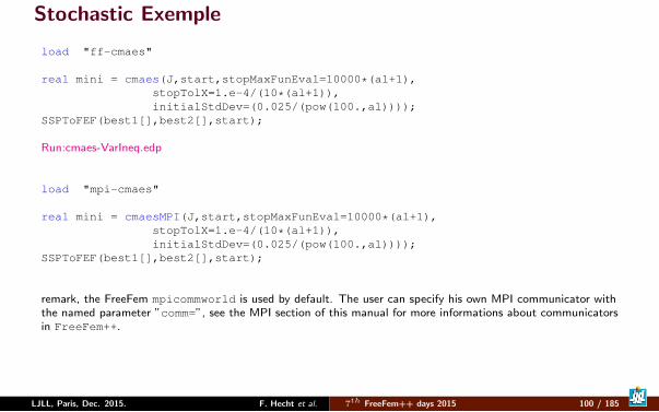
Stochastic Exemple
load "ff-cmaes"
real mini = cmaes(J,start,stopMaxFunEval=10000*(al+1),stopTolX=1.e-4/(10*(al+1)),initialStdDev=(0.025/(pow(100.,al))));
SSPToFEF(best1[],best2[],start);
Run:cmaes-VarIneq.edp
load "mpi-cmaes"
real mini = cmaesMPI(J,start,stopMaxFunEval=10000*(al+1),stopTolX=1.e-4/(10*(al+1)),initialStdDev=(0.025/(pow(100.,al))));
SSPToFEF(best1[],best2[],start);
remark, the FreeFem mpicommworld is used by default. The user can specify his own MPI communicator withthe named parameter ”comm=”, see the MPI section of this manual for more informations about communicatorsin FreeFem++.
LJLL, Paris, Dec. 2015. F. Hecht et al. 7th FreeFem++ days 2015 100 / 185
Outline
4 Numerics ToolsConnectivityInput/OutputTricksEigenvalueOptimization ToolsMPI/Parallel
LJLL, Paris, Dec. 2015. F. Hecht et al. 7th FreeFem++ days 2015 101 / 185
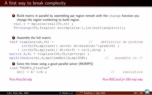
A first way to break complexity
1 Build matrix in parallel by assembling par region remark with the change function youchange the region numbering to build region.
real c = mpisize/real(Th.nt) ;Th=change(Th,fregion= min(mpisize-1,int(nuTriangle*c)));
2 Assemble the full matrixvarf vlaplace(uh,vh) = // definition de problem
int3d(Th,mpirank)( uh*vh+ dt*Grad(uh)’*grad(vh) )+ int3d(Th,mpirank)( dt*vh*f) + on(1,uh=g) ;
matrix A,Ai = vlaplace(Vh,Vh,tgv=ttgv) ;mpiAllReduce(Ai,A,mpiCommWorld,mpiSUM); // assemble in //
3 Solve the linear using a good parallel solver (MUMPS)load "MUMPS_FreeFem"
uh[] = Aˆ-1*b ; // resolution
Run:Heat3d.edp Run:NSCaraCyl-100-mpi.edp
LJLL, Paris, Dec. 2015. F. Hecht et al. 7th FreeFem++ days 2015 102 / 185
Outline
1 Introduction
2 Tools
3 Academic Examples
4 Numerics Tools
5 Schwarz method with overlap
6 Exercices
7 No Linear Problem
8 Technical Remark on freefem++
LJLL, Paris, Dec. 2015. F. Hecht et al. 7th FreeFem++ days 2015 103 / 185
Outline
5 Schwarz method with overlapPoisson equation with Schwarz methodTransfer Partparallel GMRESA simple Coarse grid solverNumerical experiment
LJLL, Paris, Dec. 2015. F. Hecht et al. 7th FreeFem++ days 2015 104 / 185
Poisson equation with Schwarz method
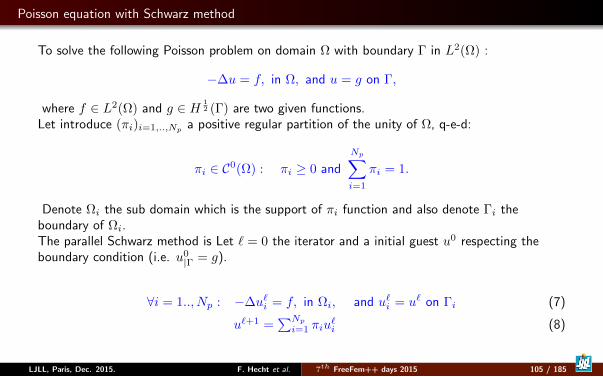
To solve the following Poisson problem on domain Ω with boundary Γ in L2(Ω) :
−∆u = f, in Ω, and u = g on Γ,
where f ∈ L2(Ω) and g ∈ H 12 (Γ) are two given functions.
Let introduce (πi)i=1,..,Np a positive regular partition of the unity of Ω, q-e-d:
πi ∈ C0(Ω) : πi ≥ 0 and
Np∑i=1
πi = 1.
Denote Ωi the sub domain which is the support of πi function and also denote Γi theboundary of Ωi.The parallel Schwarz method is Let ` = 0 the iterator and a initial guest u0 respecting theboundary condition (i.e. u0
|Γ = g).
∀i = 1.., Np : −∆u`i = f, in Ωi, and u`i = u` on Γi (7)
u`+1 =∑Np
i=1 πiu`i (8)
LJLL, Paris, Dec. 2015. F. Hecht et al. 7th FreeFem++ days 2015 105 / 185
Some Remark
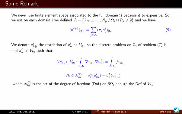
We never use finite element space associated to the full domain Ω because it to expensive. Sowe use on each domain i we defined Ji = j ∈ 1, . . . , Np / Ωi ∩ Ωj 6= ∅ and we have
(u`+1)|Ωi=∑j∈Ji
(πju`j)|Ωi
(9)
We denote u`h|i the restriction of u`h on Vhi, so the discrete problem on Ωi of problem (7) is
find u`hi ∈ Vhi such that:
∀vhi ∈ V0i :
∫Ωi
∇vhi.∇u`hi =
∫Ωi
fvhi,
∀k ∈ NΓi
hi : σki (u`hi) = σki (u`h|i)
where NΓi
hi is the set of the degree of freedom (Dof) on ∂Ωi and σki the Dof of Vhi.
LJLL, Paris, Dec. 2015. F. Hecht et al. 7th FreeFem++ days 2015 106 / 185
Outline
5 Schwarz method with overlapPoisson equation with Schwarz methodTransfer Partparallel GMRESA simple Coarse grid solverNumerical experiment
LJLL, Paris, Dec. 2015. F. Hecht et al. 7th FreeFem++ days 2015 107 / 185
Transfer Part equation(5)
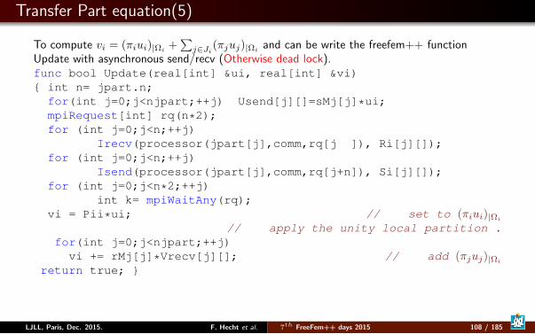
To compute vi = (πiui)|Ωi+∑j∈Ji(πjuj)|Ωi
and can be write the freefem++ functionUpdate with asynchronous send/recv (Otherwise dead lock).func bool Update(real[int] &ui, real[int] &vi) int n= jpart.n;
for(int j=0;j<njpart;++j) Usend[j][]=sMj[j]*ui;mpiRequest[int] rq(n*2);for (int j=0;j<n;++j)
Irecv(processor(jpart[j],comm,rq[j ]), Ri[j][]);for (int j=0;j<n;++j)
Isend(processor(jpart[j],comm,rq[j+n]), Si[j][]);for (int j=0;j<n*2;++j)
int k= mpiWaitAny(rq);vi = Pii*ui; // set to (πiui)|Ωi
// apply the unity local partition .for(int j=0;j<njpart;++j)
vi += rMj[j]*Vrecv[j][]; // add (πjuj)|Ωi
return true;
LJLL, Paris, Dec. 2015. F. Hecht et al. 7th FreeFem++ days 2015 108 / 185
Outline
5 Schwarz method with overlapPoisson equation with Schwarz methodTransfer Partparallel GMRESA simple Coarse grid solverNumerical experiment
LJLL, Paris, Dec. 2015. F. Hecht et al. 7th FreeFem++ days 2015 109 / 185
parallel GMRES
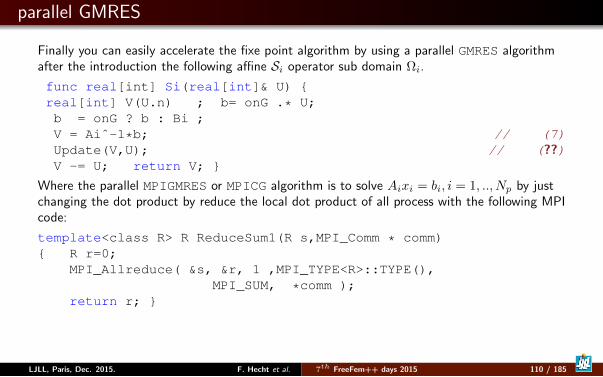
Finally you can easily accelerate the fixe point algorithm by using a parallel GMRES algorithmafter the introduction the following affine Si operator sub domain Ωi.
func real[int] Si(real[int]& U) real[int] V(U.n) ; b= onG .* U;b = onG ? b : Bi ;V = Aiˆ-1*b; // (7)Update(V,U); // (??)V -= U; return V;
Where the parallel MPIGMRES or MPICG algorithm is to solve Aixi = bi, i = 1, .., Np by justchanging the dot product by reduce the local dot product of all process with the following MPIcode:
template<class R> R ReduceSum1(R s,MPI_Comm * comm) R r=0;
MPI_Allreduce( &s, &r, 1 ,MPI_TYPE<R>::TYPE(),MPI_SUM, *comm );
return r;
LJLL, Paris, Dec. 2015. F. Hecht et al. 7th FreeFem++ days 2015 110 / 185
Outline
5 Schwarz method with overlapPoisson equation with Schwarz methodTransfer Partparallel GMRESA simple Coarse grid solverNumerical experiment
LJLL, Paris, Dec. 2015. F. Hecht et al. 7th FreeFem++ days 2015 111 / 185
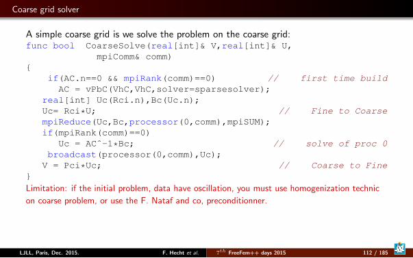
Coarse grid solver
A simple coarse grid is we solve the problem on the coarse grid:func bool CoarseSolve(real[int]& V,real[int]& U,
mpiComm& comm)
if(AC.n==0 && mpiRank(comm)==0) // first time buildAC = vPbC(VhC,VhC,solver=sparsesolver);
real[int] Uc(Rci.n),Bc(Uc.n);Uc= Rci*U; // Fine to CoarsempiReduce(Uc,Bc,processor(0,comm),mpiSUM);if(mpiRank(comm)==0)
Uc = ACˆ-1*Bc; // solve of proc 0broadcast(processor(0,comm),Uc);
V = Pci*Uc; // Coarse to Fine
Limitation: if the initial problem, data have oscillation, you must use homogenization technic
on coarse problem, or use the F. Nataf and co, preconditionner.
LJLL, Paris, Dec. 2015. F. Hecht et al. 7th FreeFem++ days 2015 112 / 185
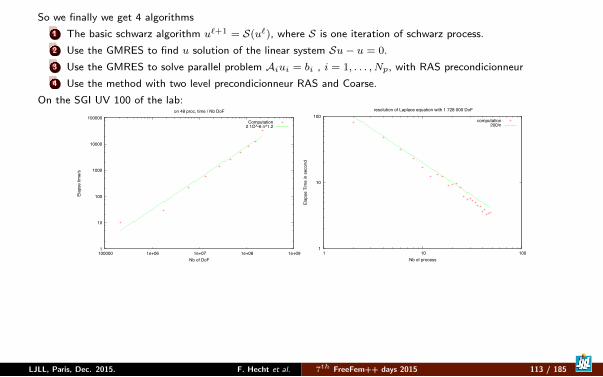
So we finally we get 4 algorithms
1 The basic schwarz algorithm u`+1 = S(u`), where S is one iteration of schwarz process.
2 Use the GMRES to find u solution of the linear system Su− u = 0.
3 Use the GMRES to solve parallel problem Aiui = bi , i = 1, . . . , Np, with RAS precondicionneur
4 Use the method with two level precondicionneur RAS and Coarse.
On the SGI UV 100 of the lab:
1
10
100
1000
10000
100000
100000 1e+06 1e+07 1e+08 1e+09
Elap
se ti
me/
s
Nb of DoF
on 48 proc, time / Nb DoF
Computation2 1O^-6 n^1.2
1
10
100
1 10 100
Elap
se T
ime
in s
econ
d
Nb of process
resolution of Laplace equation with 1 728 000 DoF
computation200/n
LJLL, Paris, Dec. 2015. F. Hecht et al. 7th FreeFem++ days 2015 113 / 185

Outline
5 Schwarz method with overlapPoisson equation with Schwarz methodTransfer Partparallel GMRESA simple Coarse grid solverNumerical experiment
LJLL, Paris, Dec. 2015. F. Hecht et al. 7th FreeFem++ days 2015 114 / 185
A Parallel Numerical experiment on laptop
We consider first example in an academic situation to solve Poisson Problem on thecube Ω =]0, 1[3
−∆u = 1, in Ω; u = 0, on ∂Ω. (10)
With a cartesian meshes Thn of Ω with 6n3 tetrahedron, the coarse mesh is Th∗m, andm is a divisor of n.We do the validation of the algorithm on a Laptop Intel Core i7 with 4 core at 1.8 Ghzwith 4Go of RAM DDR3 at 1067 Mhz,
Run:DDM-Schwarz-Lap-2dd.edp Run:DDM-Schwarz-Lame-2d.edpRun:DDM-Schwarz-Lame-3d.edp Run:DDM-Schwarz-Stokes-2d.edp
LJLL, Paris, Dec. 2015. F. Hecht et al. 7th FreeFem++ days 2015 115 / 185
Outline
1 Introduction
2 Tools
3 Academic Examples
4 Numerics Tools
5 Schwarz method with overlap
6 Exercices
7 No Linear Problem
8 Technical Remark on freefem++
LJLL, Paris, Dec. 2015. F. Hecht et al. 7th FreeFem++ days 2015 116 / 185
Outline
6 ExercicesAn exercice: Oven problemAn exercice: Min surface problemHeat equation with thermic resistanceBenchmark: Navier-Stokes
LJLL, Paris, Dec. 2015. F. Hecht et al. 7th FreeFem++ days 2015 117 / 185
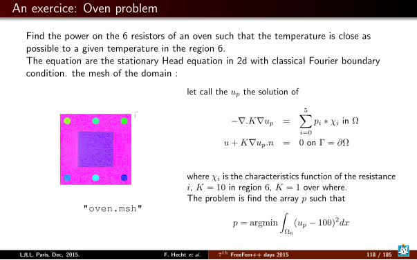
An exercice: Oven problem
Find the power on the 6 resistors of an oven such that the temperature is close aspossible to a given temperature in the region 6.The equation are the stationary Head equation in 2d with classical Fourier boundarycondition. the mesh of the domain :
IsoValue012345678
"oven.msh"
let call the up the solution of
−∇.K∇up =
5∑i=0
pi ∗ χi in Ω
u+K∇up.n = 0 on Γ = ∂Ω
where χi is the characteristics function of the resistancei, K = 10 in region 6, K = 1 over where.The problem is find the array p such that
p = argmin
∫Ω6
(up − 100)2dx
LJLL, Paris, Dec. 2015. F. Hecht et al. 7th FreeFem++ days 2015 118 / 185
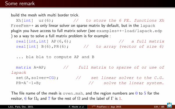
Some remark
build the mesh with multi border trick.Xh[int] ur(6); // to store the 6 FE. functions Xh
FreeFem++ as only linear solver on sparse matrix by default, but in the lapackplugin you have access to full matrix solver (see examples++-load/lapack.edp) so a way to solve a full matrix problem is for example :real[int,int] AP(6,6); // a full matrixreal[int] B(6),PR(6); // to array (vector of size 6)
... bla bla to compute AP and B
matrix A=AP; // full matrix to sparse of or use oflapackset(A,solver=CG); // set linear solver to the C.G.PR=Aˆ-1*B; // solve the linear system.
The file name of the mesh is oven.msh, and the region numbers are 0 to 5 for theresitor, 6 for Ω6 and 7 for the rest of Ω and the label of Γ is 1.
LJLL, Paris, Dec. 2015. F. Hecht et al. 7th FreeFem++ days 2015 119 / 185
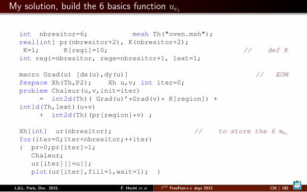
My solution, build the 6 basics function uei
int nbresitor=6; mesh Th("oven.msh");real[int] pr(nbresitor+2), K(nbresitor+2);K=1; K[regi]=10; // def K
int regi=nbresitor, rege=nbresitor+1, lext=1;
macro Grad(u) [dx(u),dy(u)] // EOMfespace Xh(Th,P2); Xh u,v; int iter=0;problem Chaleur(u,v,init=iter)
= int2d(Th)( Grad(u)’*Grad(v)* K[region]) +int1d(Th,lext)(u*v)
+ int2d(Th)(pr[region]*v) ;
Xh[int] ur(nbresitor); // to store the 6 ueifor(iter=0;iter<nbresitor;++iter) pr=0;pr[iter]=1;
Chaleur;ur[iter][]=u[];plot(ur[iter],fill=1,wait=1);
LJLL, Paris, Dec. 2015. F. Hecht et al. 7th FreeFem++ days 2015 120 / 185
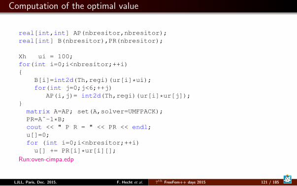
Computation of the optimal value
real[int,int] AP(nbresitor,nbresitor);real[int] B(nbresitor),PR(nbresitor);
Xh ui = 100;for(int i=0;i<nbresitor;++i)
B[i]=int2d(Th,regi)(ur[i]*ui);for(int j=0;j<6;++j)
AP(i,j)= int2d(Th,regi)(ur[i]*ur[j]);
matrix A=AP; set(A,solver=UMFPACK);PR=Aˆ-1*B;cout << " P R = " << PR << endl;u[]=0;for (int i=0;i<nbresitor;++i)
u[] += PR[i]*ur[i][];
Run:oven-cimpa.edp
LJLL, Paris, Dec. 2015. F. Hecht et al. 7th FreeFem++ days 2015 121 / 185
Outline
6 ExercicesAn exercice: Oven problemAn exercice: Min surface problemHeat equation with thermic resistanceBenchmark: Navier-Stokes
LJLL, Paris, Dec. 2015. F. Hecht et al. 7th FreeFem++ days 2015 122 / 185
An exercice: Min surface problem
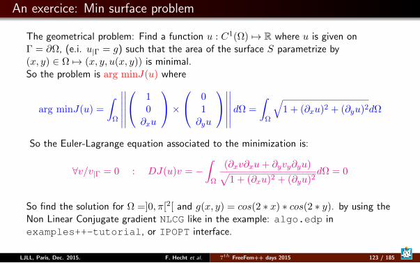
The geometrical problem: Find a function u : C1(Ω) 7→ R where u is given onΓ = ∂Ω, (e.i. u|Γ = g) such that the area of the surface S parametrize by(x, y) ∈ Ω 7→ (x, y, u(x, y)) is minimal.So the problem is arg minJ(u) where
arg minJ(u) =
∫Ω
∣∣∣∣∣∣∣∣∣∣∣∣ 1
0∂xu
× 0
1∂yu
∣∣∣∣∣∣∣∣∣∣∣∣ dΩ =
∫Ω
√1 + (∂xu)2 + (∂yu)2dΩ
So the Euler-Lagrange equation associated to the minimization is:
∀v/v|Γ = 0 : DJ(u)v = −∫
Ω
(∂xv∂xu+ ∂yvy∂yu)√1 + (∂xu)2 + (∂yu)2
dΩ = 0
So find the solution for Ω =]0, π[2[ and g(x, y) = cos(2 ∗ x) ∗ cos(2 ∗ y). by using theNon Linear Conjugate gradient NLCG like in the example: algo.edp inexamples++-tutorial, or IPOPT interface.
LJLL, Paris, Dec. 2015. F. Hecht et al. 7th FreeFem++ days 2015 123 / 185
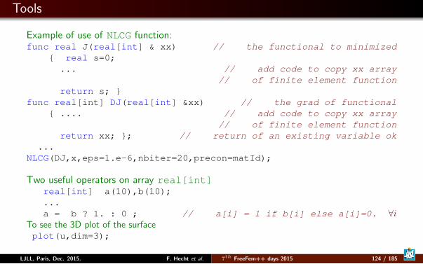
Tools
Example of use of NLCG function:func real J(real[int] & xx) // the functional to minimized
real s=0;... // add code to copy xx array
// of finite element functionreturn s;
func real[int] DJ(real[int] &xx) // the grad of functional .... // add code to copy xx array
// of finite element functionreturn xx; ; // return of an existing variable ok
...NLCG(DJ,x,eps=1.e-6,nbiter=20,precon=matId);
Two useful operators on array real[int]real[int] a(10),b(10);...a = b ? 1. : 0 ; // a[i] = 1 if b[i] else a[i]=0. ∀i
To see the 3D plot of the surfaceplot(u,dim=3);
LJLL, Paris, Dec. 2015. F. Hecht et al. 7th FreeFem++ days 2015 124 / 185
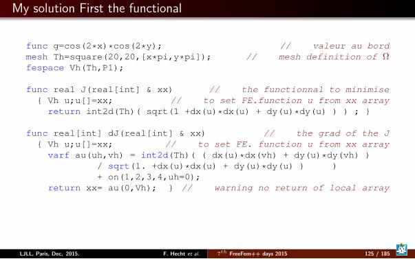
My solution First the functional
func g=cos(2*x)*cos(2*y); // valeur au bordmesh Th=square(20,20,[x*pi,y*pi]); // mesh definition of Ωfespace Vh(Th,P1);
func real J(real[int] & xx) // the functionnal to minimise Vh u;u[]=xx; // to set FE.function u from xx array
return int2d(Th)( sqrt(1 +dx(u)*dx(u) + dy(u)*dy(u) ) ) ;
func real[int] dJ(real[int] & xx) // the grad of the J Vh u;u[]=xx; // to set FE. function u from xx arrayvarf au(uh,vh) = int2d(Th)( ( dx(u)*dx(vh) + dy(u)*dy(vh) )
/ sqrt(1. +dx(u)*dx(u) + dy(u)*dy(u) ) )+ on(1,2,3,4,uh=0);
return xx= au(0,Vh); // warning no return of local array
LJLL, Paris, Dec. 2015. F. Hecht et al. 7th FreeFem++ days 2015 125 / 185
My solution Second the call
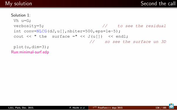
Solution 1:Vh u=G;verbosity=5; // to see the residualint conv=NLCG(dJ,u[],nbiter=500,eps=1e-5);cout << " the surface =" << J(u[]) << endl;
// so see the surface un 3Dplot(u,dim=3);
Run:minimal-surf.edp
LJLL, Paris, Dec. 2015. F. Hecht et al. 7th FreeFem++ days 2015 126 / 185
Outline
6 ExercicesAn exercice: Oven problemAn exercice: Min surface problemHeat equation with thermic resistanceBenchmark: Navier-Stokes
LJLL, Paris, Dec. 2015. F. Hecht et al. 7th FreeFem++ days 2015 127 / 185
Heat equation with thermic resistance
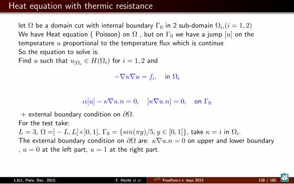
let Ω be a domain cut with internal boundary Γ0 in 2 sub-domain Ωi,(i = 1, 2)We have Heat equation ( Poisson) on Ω , but on Γ0 we have a jump [u] on thetemperature u proportional to the temperature flux which is continueSo the equation to solve is:Find u such that u|Ωi
∈ H(Ωi) for i = 1, 2 and
−∇κ∇u = fi, in Ωi
α[u]− κ∇u.n = 0, [κ∇u.n] = 0, on Γ0
+ external boundary condition on ∂Ω.For the test take:L = 3, Ω =]− L,L[×]0, 1[, Γ0 = sin(πy)/5, y ∈ [0, 1], take κ = i in Ωi.The external boundary condition on ∂Ω are: κ∇u.n = 0 on upper and lower boundary, u = 0 at the left part, u = 1 at the right part.
LJLL, Paris, Dec. 2015. F. Hecht et al. 7th FreeFem++ days 2015 128 / 185
Heat equation with thermic resistance
Method 1: Solve 2 coupled problems and use the block matrix tools to defined thelinear system of the problem.Method 2: We suppose the Γ0 move with time, and Γ0 is not discretize in the mesh.
LJLL, Paris, Dec. 2015. F. Hecht et al. 7th FreeFem++ days 2015 129 / 185
Outline
6 ExercicesAn exercice: Oven problemAn exercice: Min surface problemHeat equation with thermic resistanceBenchmark: Navier-Stokes
LJLL, Paris, Dec. 2015. F. Hecht et al. 7th FreeFem++ days 2015 130 / 185
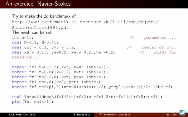
An exercice: Navier-Stokes
Try to make the 2d benchmark of :http://www.mathematik.tu-dortmund.de/lsiii/cms/papers/SchaeferTurek1996.pdfThe mesh can be set:int n=15; // parameter ...real D=0.1, H=0.41;real cx0 = 0.2, cy0 = 0.2; // center of cyl.real xa = 0.15, ya=0.2, xe = 0.25,ye =0.2; // point forpressure..
border fr1(t=0,2.2)x=t; y=0; label=1;border fr2(t=0,H)x=2.2; y=t; label=2;border fr3(t=2.2,0)x=t; y=H; label=1;border fr4(t=H,0)x=0; y=t; label=1;border fr5(t=2*pi,0)x=cx0+D*sin(t)/2; y=cy0+D*cos(t)/2; label=3;
mesh Th=buildmesh(fr1(5*n)+fr2(n)+fr3(5*n)+fr4(n)+fr5(-n*3));plot(Th, wait=1);
LJLL, Paris, Dec. 2015. F. Hecht et al. 7th FreeFem++ days 2015 131 / 185
Outline
1 Introduction
2 Tools
3 Academic Examples
4 Numerics Tools
5 Schwarz method with overlap
6 Exercices
7 No Linear Problem
8 Technical Remark on freefem++
LJLL, Paris, Dec. 2015. F. Hecht et al. 7th FreeFem++ days 2015 132 / 185
Outline
7 No Linear ProblemNewton MethodNavier-StokesVariational InequalityGround waterBose Einstein CondensateHyper elasticity equationPeriodic Surface Acoustic Waves Transducer AnalysisPhase change with Natural Convection
LJLL, Paris, Dec. 2015. F. Hecht et al. 7th FreeFem++ days 2015 133 / 185
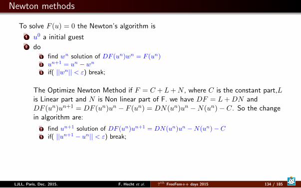
Newton methods
To solve F (u) = 0 the Newton’s algorithm is
1 u0 a initial guest2 do
1 find wn solution of DF (un)wn = F (un)2 un+1 = un − wn3 if( ||wn|| < ε) break;
The Optimize Newton Method if F = C +L+N , where C is the constant part,Lis Linear part and N is Non linear part of F. we have DF = L+DN andDF (un)un+1 = DF (un)un − F (un) = DN(un)un −N(un)− C. So the changein algorithm are:
2 find un+1 solution of DF (un)un+1 = DN(un)un −N(un)− C3 if( ||un+1 − un|| < ε) break;
LJLL, Paris, Dec. 2015. F. Hecht et al. 7th FreeFem++ days 2015 134 / 185
Outline
7 No Linear ProblemNewton MethodNavier-StokesVariational InequalityGround waterBose Einstein CondensateHyper elasticity equationPeriodic Surface Acoustic Waves Transducer AnalysisPhase change with Natural Convection
LJLL, Paris, Dec. 2015. F. Hecht et al. 7th FreeFem++ days 2015 135 / 185
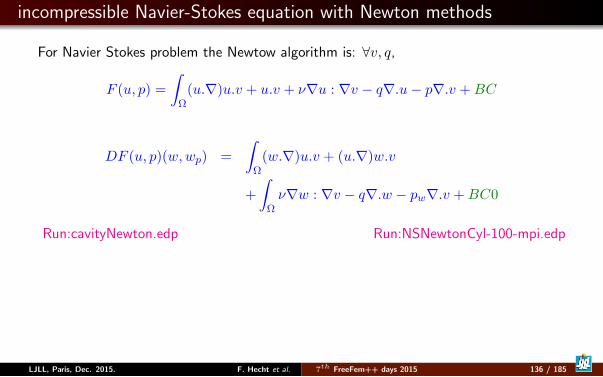
incompressible Navier-Stokes equation with Newton methods
For Navier Stokes problem the Newtow algorithm is: ∀v, q,
F (u, p) =
∫Ω
(u.∇)u.v + u.v + ν∇u : ∇v − q∇.u− p∇.v +BC
DF (u, p)(w,wp) =
∫Ω
(w.∇)u.v + (u.∇)w.v
+
∫Ων∇w : ∇v − q∇.w − pw∇.v +BC0
Run:cavityNewton.edp Run:NSNewtonCyl-100-mpi.edp
LJLL, Paris, Dec. 2015. F. Hecht et al. 7th FreeFem++ days 2015 136 / 185
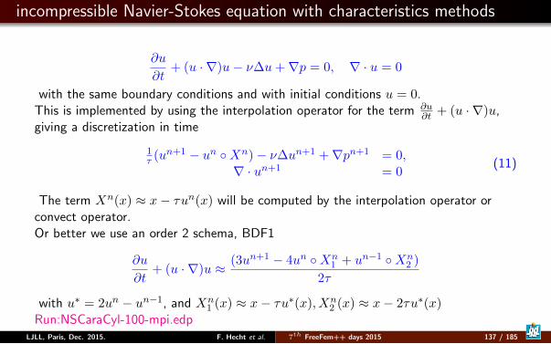
incompressible Navier-Stokes equation with characteristics methods
∂u
∂t+ (u · ∇)u− ν∆u+∇p = 0, ∇ · u = 0
with the same boundary conditions and with initial conditions u = 0.This is implemented by using the interpolation operator for the term ∂u
∂t + (u · ∇)u,giving a discretization in time
1τ (un+1 − un Xn)− ν∆un+1 +∇pn+1 = 0,
∇ · un+1 = 0(11)
The term Xn(x) ≈ x− τun(x) will be computed by the interpolation operator orconvect operator.Or better we use an order 2 schema, BDF1
∂u
∂t+ (u · ∇)u ≈ (3un+1 − 4un Xn
1 + un−1 Xn2 )
2τ
with u∗ = 2un − un−1, and Xn1 (x) ≈ x− τu∗(x), Xn
2 (x) ≈ x− 2τu∗(x)Run:NSCaraCyl-100-mpi.edp
LJLL, Paris, Dec. 2015. F. Hecht et al. 7th FreeFem++ days 2015 137 / 185
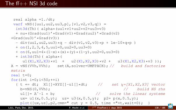
The ff++ NSI 3d code
real alpha =1./dt;varf vNS([uu1,uu2,uu3,p],[v1,v2,v3,q]) =int3d(Th)( alpha*(uu1*v1+uu2*v2+uu3*v3)+ nu*(Grad(uu1)’*Grad(v1)+Grad(uu2)’*Grad(v2)
+Grad(uu3)’*Grad(v3))- div(uu1,uu2,uu3)*q - div(v1,v2,v3)*p + 1e-10*q*p )+ on(1,2,3,4,5,uu1=0,uu2=0,uu3=0)+ on(6,uu1=4*(1-x)*(x)*(y)*(1-y),uu2=0,uu3=0)+ int3d(Th)( alpha*(
u1(X1,X2,X3)*v1 + u2(X1,X2,X3)*v2 + u3(X1,X2,X3)*v3 ));A = vNS(VVh,VVh); set(A,solver=UMFPACK); // build and factorizematrixreal t=0;for(int i=0;i<50;++i)
t += dt; X1[]=XYZ[]-u1[]*dt; // set χ=[X1,X2,X3] vectorb=vNS(0,VVh); // build NS rhsu1[]= Aˆ-1 * b; // solve the linear systemeux= u1(x,0.5,y); uz= u3(x,0.5,y); p2= p(x,0.5,y);plot([ux,uz],p2,cmm=" cut y = 0.5, time ="+t,wait=0);
Run:NSI3d.edpLJLL, Paris, Dec. 2015. F. Hecht et al. 7th FreeFem++ days 2015 138 / 185
Outline
7 No Linear ProblemNewton MethodNavier-StokesVariational InequalityGround waterBose Einstein CondensateHyper elasticity equationPeriodic Surface Acoustic Waves Transducer AnalysisPhase change with Natural Convection
LJLL, Paris, Dec. 2015. F. Hecht et al. 7th FreeFem++ days 2015 139 / 185
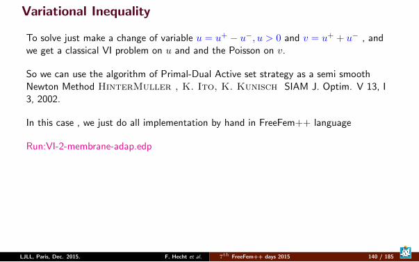
Variational Inequality
To solve just make a change of variable u = u+ − u−, u > 0 and v = u+ + u− , andwe get a classical VI problem on u and and the Poisson on v.
So we can use the algorithm of Primal-Dual Active set strategy as a semi smoothNewton Method HinterMuller , K. Ito, K. Kunisch SIAM J. Optim. V 13, I3, 2002.
In this case , we just do all implementation by hand in FreeFem++ language
Run:VI-2-membrane-adap.edp
LJLL, Paris, Dec. 2015. F. Hecht et al. 7th FreeFem++ days 2015 140 / 185
Outline
7 No Linear ProblemNewton MethodNavier-StokesVariational InequalityGround waterBose Einstein CondensateHyper elasticity equationPeriodic Surface Acoustic Waves Transducer AnalysisPhase change with Natural Convection
LJLL, Paris, Dec. 2015. F. Hecht et al. 7th FreeFem++ days 2015 141 / 185
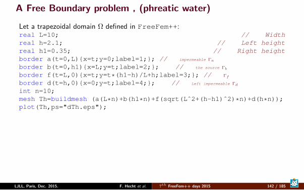
A Free Boundary problem , (phreatic water)
Let a trapezoidal domain Ω defined in FreeFem++:real L=10; // Widthreal h=2.1; // Left heightreal h1=0.35; // Right heightborder a(t=0,L)x=t;y=0;label=1;; // impermeable Γa
border b(t=0,h1)x=L;y=t;label=2;; // the source Γb
border f(t=L,0)x=t;y=t*(h1-h)/L+h;label=3;; // Γf
border d(t=h,0)x=0;y=t;label=4;; // Left impermeable Γd
int n=10;mesh Th=buildmesh (a(L*n)+b(h1*n)+f(sqrt(Lˆ2+(h-h1)ˆ2)*n)+d(h*n));plot(Th,ps="dTh.eps");
LJLL, Paris, Dec. 2015. F. Hecht et al. 7th FreeFem++ days 2015 142 / 185
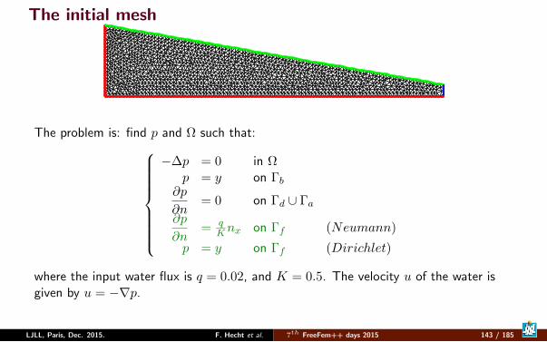
The initial mesh
The problem is: find p and Ω such that:
−∆p = 0 in Ωp = y on Γb
∂p
∂n= 0 on Γd ∪ Γa
∂p
∂n= q
Knx on Γf (Neumann)
p = y on Γf (Dirichlet)
where the input water flux is q = 0.02, and K = 0.5. The velocity u of the water isgiven by u = −∇p.
LJLL, Paris, Dec. 2015. F. Hecht et al. 7th FreeFem++ days 2015 143 / 185
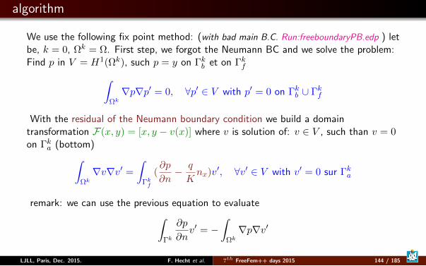
algorithm
We use the following fix point method: (with bad main B.C. Run:freeboundaryPB.edp ) letbe, k = 0, Ωk = Ω. First step, we forgot the Neumann BC and we solve the problem:Find p in V = H1(Ωk), such p = y on Γkb et on Γkf∫
Ωk
∇p∇p′ = 0, ∀p′ ∈ V with p′ = 0 on Γkb ∪ Γkf
With the residual of the Neumann boundary condition we build a domaintransformation F(x, y) = [x, y − v(x)] where v is solution of: v ∈ V , such than v = 0on Γka (bottom)∫
Ωk
∇v∇v′ =∫
Γkf
(∂p
∂n− q
Knx)v′, ∀v′ ∈ V with v′ = 0 sur Γka
remark: we can use the previous equation to evaluate∫Γk
∂p
∂nv′ = −
∫Ωk
∇p∇v′
LJLL, Paris, Dec. 2015. F. Hecht et al. 7th FreeFem++ days 2015 144 / 185
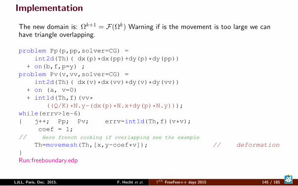
Implementation
The new domain is: Ωk+1 = F(Ωk) Warning if is the movement is too large we canhave triangle overlapping.
problem Pp(p,pp,solver=CG) =int2d(Th)( dx(p)*dx(pp)+dy(p)*dy(pp))
+ on(b,f,p=y) ;problem Pv(v,vv,solver=CG) =
int2d(Th)( dx(v)*dx(vv)+dy(v)*dy(vv))+ on (a, v=0)+ int1d(Th,f)(vv*
((Q/K)*N.y-(dx(p)*N.x+dy(p)*N.y)));while(errv>1e-6) j++; Pp; Pv; errv=int1d(Th,f)(v*v);
coef = 1;// Here french cooking if overlapping see the example
Th=movemesh(Th,[x,y-coef*v]); // deformationRun:freeboundary.edp
LJLL, Paris, Dec. 2015. F. Hecht et al. 7th FreeFem++ days 2015 145 / 185
Outline
7 No Linear ProblemNewton MethodNavier-StokesVariational InequalityGround waterBose Einstein CondensateHyper elasticity equationPeriodic Surface Acoustic Waves Transducer AnalysisPhase change with Natural Convection
LJLL, Paris, Dec. 2015. F. Hecht et al. 7th FreeFem++ days 2015 146 / 185
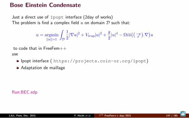
Bose Einstein Condensate
Just a direct use of Ipopt interface (2day of works)The problem is find a complex field u on domain D such that:
u = argmin||u||=1
∫D
1
2|∇u|2 + Vtrap|u|2 +
g
2|u|4 − Ωiu
((−yx
).∇)u
to code that in FreeFem++use
Ipopt interface ( https://projects.coin-or.org/Ipopt)
Adaptation de maillage
Run:BEC.edp
LJLL, Paris, Dec. 2015. F. Hecht et al. 7th FreeFem++ days 2015 147 / 185

Outline
7 No Linear ProblemNewton MethodNavier-StokesVariational InequalityGround waterBose Einstein CondensateHyper elasticity equationPeriodic Surface Acoustic Waves Transducer AnalysisPhase change with Natural Convection
LJLL, Paris, Dec. 2015. F. Hecht et al. 7th FreeFem++ days 2015 148 / 185
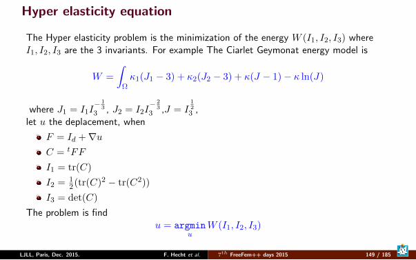
Hyper elasticity equation
The Hyper elasticity problem is the minimization of the energy W (I1, I2, I3) whereI1, I2, I3 are the 3 invariants. For example The Ciarlet Geymonat energy model is
W =
∫Ωκ1(J1 − 3) + κ2(J2 − 3) + κ(J − 1)− κ ln(J)
where J1 = I1I− 1
33 , J2 = I2I
− 23
3 ,J = I123 ,
let u the deplacement, when
F = Id +∇uC = tFF
I1 = tr(C)
I2 = 12(tr(C)2 − tr(C2))
I3 = det(C)
The problem is findu = argmin
uW (I1, I2, I3)
LJLL, Paris, Dec. 2015. F. Hecht et al. 7th FreeFem++ days 2015 149 / 185
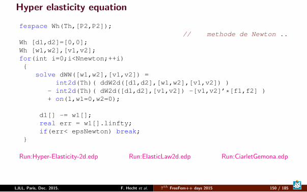
Hyper elasticity equation
fespace Wh(Th,[P2,P2]);// methode de Newton ..
Wh [d1,d2]=[0,0];Wh [w1,w2],[v1,v2];for(int i=0;i<Nnewton;++i)
solve dWW([w1,w2],[v1,v2]) =int2d(Th)( ddW2d([d1,d2],[w1,w2],[v1,v2]) )
- int2d(Th)( dW2d([d1,d2],[v1,v2]) -[v1,v2]’*[f1,f2] )+ on(1,w1=0,w2=0);
d1[] -= w1[];real err = w1[].linfty;if(err< epsNewton) break;
Run:Hyper-Elasticity-2d.edp Run:ElasticLaw2d.edp Run:CiarletGemona.edp
LJLL, Paris, Dec. 2015. F. Hecht et al. 7th FreeFem++ days 2015 150 / 185
Outline
7 No Linear ProblemNewton MethodNavier-StokesVariational InequalityGround waterBose Einstein CondensateHyper elasticity equationPeriodic Surface Acoustic Waves Transducer AnalysisPhase change with Natural Convection
LJLL, Paris, Dec. 2015. F. Hecht et al. 7th FreeFem++ days 2015 151 / 185
Periodic Surface Acoustic Waves Transducer Analysis
A true industrial numerical problem (2d) :
1 3 EDP: Dielectric, Elasticity, Piezoelectric , Linear, harmonic approximation
2 α-periodic B.C. (New simple idea)
3 semi-infinite Dielectric domain (classical Fourier/Floquet transforme)
4 semi-infinite Piezoelectric domain (Hard)
In 9 month, we build with P. Ventura (100%, me 10%) a numerical simulator form scratch (8
months for the validation), The only thing to add to freefem++ is a interface with lapack to
compute eigenvector of full 8× 8 matrix.
A good message : Les calculs des parametres physiques des transducteurs dans la banded’arret et les evaluations de capacite statiques sont tres satisfaisants par rapport aux resultatsexperimentaux !
LJLL, Paris, Dec. 2015. F. Hecht et al. 7th FreeFem++ days 2015 152 / 185
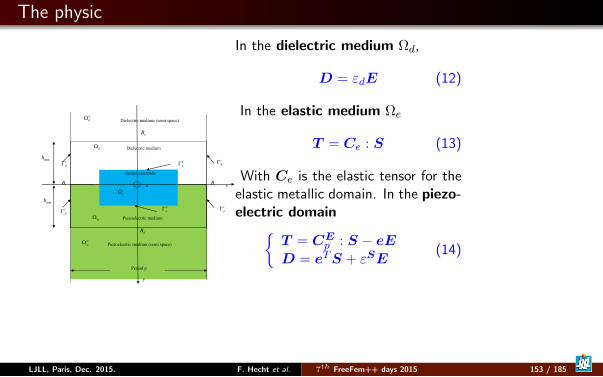
The physic
Dielectric medium (semi space)
x
maxh
minh e:
p:
d:
Period p
y
z
uB
dB
df:
pf:
rB lB
Dielectric medium
Buried electrode
Piezoelectric medium
Piezoelectric medium (semi space)
ue*
de* r
p* lp*
rd* l
d*
In the dielectric medium Ωd,
D = εdE (12)
In the elastic medium Ωe
T = Ce : S (13)
With Ce is the elastic tensor for theelastic metallic domain. In the piezo-electric domain
T = CEp : S − eE
D = eTS + εSE(14)
LJLL, Paris, Dec. 2015. F. Hecht et al. 7th FreeFem++ days 2015 153 / 185
The physic
The material domain Ωm obeys Newton’s second law:
∇ · T = ρ∂2u
∂t2(15)
The quasi static Maxwell’s equation is assumed for the whole domain Ω :
∇ ·D = 0 (16)
By using the divergence relationship and the Green’s integral formula, it results thegeneral weak formulation of the periodic γ-harmonic problem:
LJLL, Paris, Dec. 2015. F. Hecht et al. 7th FreeFem++ days 2015 154 / 185
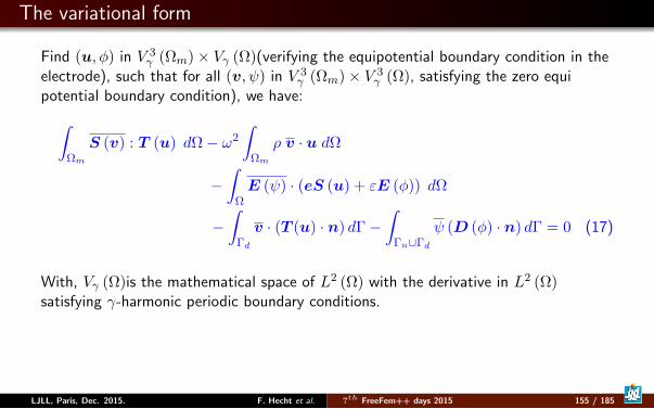
The variational form
Find (u, φ) in V 3γ (Ωm)× Vγ (Ω)(verifying the equipotential boundary condition in the
electrode), such that for all (v, ψ) in V 3γ (Ωm)× V 3
γ (Ω), satisfying the zero equipotential boundary condition), we have:∫
Ωm
S (v) : T (u) dΩ− ω2
∫Ωm
ρ v · u dΩ
−∫
ΩE (ψ) · (eS (u) + εE (φ)) dΩ
−∫
Γd
v · (T (u) · n) dΓ−∫
Γu∪Γd
ψ (D (φ) · n) dΓ = 0 (17)
With, Vγ (Ω)is the mathematical space of L2 (Ω) with the derivative in L2 (Ω)satisfying γ-harmonic periodic boundary conditions.
LJLL, Paris, Dec. 2015. F. Hecht et al. 7th FreeFem++ days 2015 155 / 185

The γ-harmonic periodic boundary trick
Let us first define ϕγ (x) = e−j2πγ x
p , ϕγ (x) is a γ-harmonic periodic functionsatisfying:
ϕγ (x+ p) = e−j2πγϕγ (x) (18)
We just do the change of variable:u (x, y) = ϕγ (x)u (x, y)φ (x, y) = ϕγ (x)φ (x, y)
(19)
Where u (x) and φ (x) are p-periodic functions.The main idea is to define a new differential operator ∇γ by:
∇γu = ∇ (ϕγu) = ϕγ∇u + ϕγ
′u (20)
Because the physical fields E,D,T , and S are expressed using partial derivative of u, and, φ,it is possible to define the operators Eγ (φ) = E (ϕγφ
), Dγ (φ) = D (ϕγφ),
Tγ (u) = T (ϕγu), ....
LJLL, Paris, Dec. 2015. F. Hecht et al. 7th FreeFem++ days 2015 156 / 185
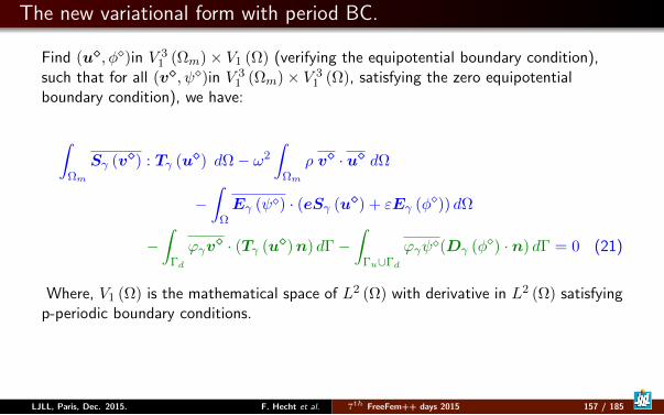
The new variational form with period BC.
Find (u, φ)in V 31 (Ωm)× V1 (Ω) (verifying the equipotential boundary condition),
such that for all (v, ψ)in V 31 (Ωm)× V 3
1 (Ω), satisfying the zero equipotentialboundary condition), we have:
∫Ωm
Sγ (v) : Tγ (u) dΩ− ω2
∫Ωm
ρ v · u dΩ
−∫
ΩEγ (ψ) · (eSγ (u) + εEγ (φ)) dΩ
−∫
Γd
ϕγv · (Tγ (u)n) dΓ−
∫Γu∪Γd
ϕγψ(Dγ (φ) · n) dΓ = 0 (21)
Where, V1 (Ω) is the mathematical space of L2 (Ω) with derivative in L2 (Ω) satisfyingp-periodic boundary conditions.
LJLL, Paris, Dec. 2015. F. Hecht et al. 7th FreeFem++ days 2015 157 / 185

BEM computation
We have to modelized the following term:
−∫
Γd
ϕγv · (Tγ (u)n) dΓ−
∫Γu∪Γd
ϕγψ(Dγ (φ) · n) dΓ, (22)
also called border terms.First from (22), let us look at the boundary integral AΓu , at the interface Γu of thesemi-infinite dielectric semi-space.
AΓu =
∫Γu
ϕγψDγ (φ) · n dΓ (23)
LJLL, Paris, Dec. 2015. F. Hecht et al. 7th FreeFem++ days 2015 158 / 185
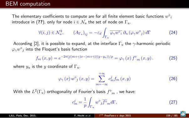
BEM computation
The elementary coefficients to compute are for all finite element basic functions wiintroduce in (??), only for node i ∈ Nu the set of node on Γu.
∀(i, j) ∈ N 2u , (AΓu)ij = −εd
∫Γu
ϕγwi ∂n (ϕγwj) dΓ (24)
According [2], it is possible to expand, at the interface Γu the γ-harmonic periodicϕγw
j into the Floquet’s basis function
fm (x, y) = e−2π(j(m+γ)x−|m+γ|((y−yu))/p = ϕγ (x) fm (x, y) . (25)
where yu is the y coordinate of Γu.
ϕγ (x)wj (x, y) =
+∞∑m=−∞
cjmfm (x, y) (26)
With the L2(Γu) orthogonality of Fourier’s basis fm , we have:
cjm =1
p
∫Γu
wjfmdΓ, (27)
LJLL, Paris, Dec. 2015. F. Hecht et al. 7th FreeFem++ days 2015 159 / 185
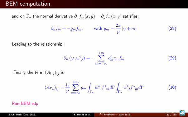
BEM computation,
and on Γu the normal derivative ∂nfm(x, y) = ∂yfm(x, y) satisfies:
∂nfm = −gmfm, with gm =2π
p|γ +m| (28)
Leading to the relationship:
∂n (ϕγwj) = −
+∞∑m=−∞
cjmgmfm (29)
Finally the term (AΓu)ij is
(AΓu)ij =εdp
+∞∑m=∞
gm
∫Γu
wifmdΓ
∫Γu
wjfmdΓ (30)
Run:BEM.edp
LJLL, Paris, Dec. 2015. F. Hecht et al. 7th FreeFem++ days 2015 160 / 185
Outline
7 No Linear ProblemNewton MethodNavier-StokesVariational InequalityGround waterBose Einstein CondensateHyper elasticity equationPeriodic Surface Acoustic Waves Transducer AnalysisPhase change with Natural Convection
LJLL, Paris, Dec. 2015. F. Hecht et al. 7th FreeFem++ days 2015 161 / 185
Phase change with Natural Convection
The starting point of the problem is Brainstorming session (part I) of the third FreeFem++days in december 2011, this is almost the Orange Problem is describe in web page http://www.ljll.math.upmc.fr/˜hecht/ftp/ff++days/2011/Orange-problem.pdf.The coupling of natural convection modeled by the Boussinesq approximation and liquid tosolid phase change in Ω =]0, 1[2, No slip condition for the fluid are applied at the boundary andadiabatic condition on upper and lower boundary and given temperature θr (resp θl) at theright and left boundaries.The model is: find the field : the velocity u = (u1, u2), the pressure p and temperature θ :
u given in Ωs∂tu + (u∇)u +∇.µ∇u +∇p = −cTe2 in Ωf
∇.u = 0 in Ωf∂tθ + (u∇)θ +∇.kT∇θ = ∂tS(T ) in Ω
(31)
Where Ωf is the fluid domain and the solid domain is Ωs = Ω \ Ωf .
LJLL, Paris, Dec. 2015. F. Hecht et al. 7th FreeFem++ days 2015 162 / 185
Phase change with Natural Convection
The enthalpy of the change of phase is given by the function S; µ is the relativeviscosity, kT the thermal diffusivity.In Ωf = x ∈ Ω; θ > θf, with θm the melting temperature the solid has melt.We modeled, the solid phase as a fluid with huge viscosity, so :
µ =
θ < θf ∼ 106
θ ≥ θm ∼ 1Re
,
The Stefan enthalpy Sc with defined by Sc(θ) = H(θ)/Sth where Sthe is the stefannumber, and H is the Heaviside function with use the following smooth the enthalpy:
S(θ) =tanh(50(θ − θm)))
2Ste.
LJLL, Paris, Dec. 2015. F. Hecht et al. 7th FreeFem++ days 2015 163 / 185
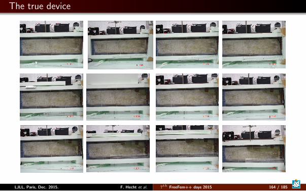
The true device
12 Etude MCPAM °52C
LJLL, Paris, Dec. 2015. F. Hecht et al. 7th FreeFem++ days 2015 164 / 185
the Algorithm
We apply a fixed point algorithm for the phase change part (the domain Ωf is fixed ateach iteration) and a full no-linear Euler implicit scheme with a fixed domain for therest. We use a Newton method to solve the non-linearity.
if we don’t make mesh adaptation, the Newton method do not converge
if we use explicit method diverge too,
if we implicit the dependance in Ωs the method also diverge.
This is a really difficult problem.
LJLL, Paris, Dec. 2015. F. Hecht et al. 7th FreeFem++ days 2015 165 / 185
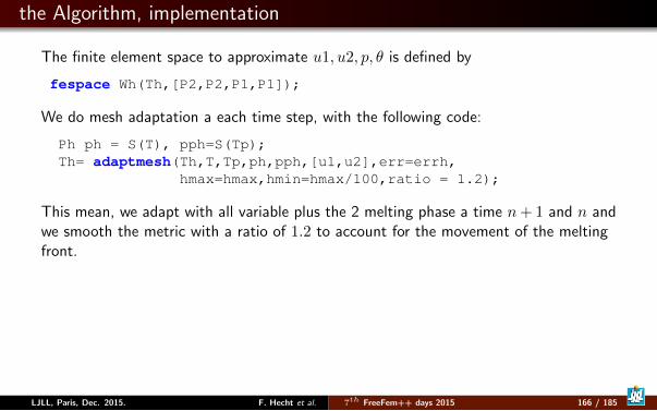
the Algorithm, implementation
The finite element space to approximate u1, u2, p, θ is defined by
fespace Wh(Th,[P2,P2,P1,P1]);
We do mesh adaptation a each time step, with the following code:
Ph ph = S(T), pph=S(Tp);Th= adaptmesh(Th,T,Tp,ph,pph,[u1,u2],err=errh,
hmax=hmax,hmin=hmax/100,ratio = 1.2);
This mean, we adapt with all variable plus the 2 melting phase a time n+ 1 and n andwe smooth the metric with a ratio of 1.2 to account for the movement of the meltingfront.
LJLL, Paris, Dec. 2015. F. Hecht et al. 7th FreeFem++ days 2015 166 / 185
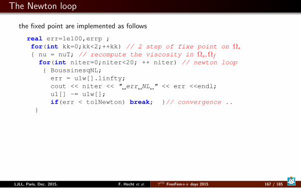
The Newton loop
the fixed point are implemented as follows
real err=1e100,errp ;for(int kk=0;kk<2;++kk) // 2 step of fixe point on Ωs nu = nuT; // recompute the viscosity in Ωs,Ωf
for(int niter=0;niter<20; ++ niter) // newton loop BoussinesqNL;
err = u1w[].linfty;cout << niter << " err NL " << err <<endl;u1[] -= u1w[];if(err < tolNewton) break; // convergence ..
LJLL, Paris, Dec. 2015. F. Hecht et al. 7th FreeFem++ days 2015 167 / 185
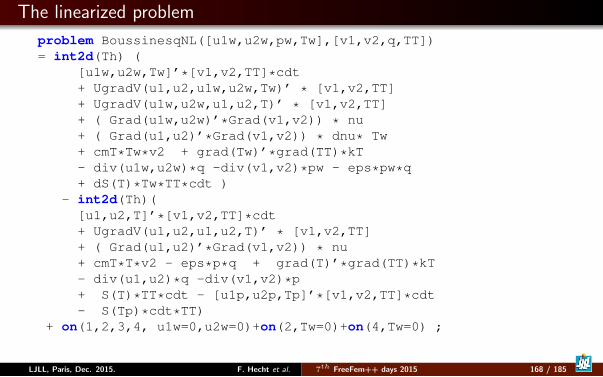
The linearized problem
problem BoussinesqNL([u1w,u2w,pw,Tw],[v1,v2,q,TT])= int2d(Th) (
[u1w,u2w,Tw]’*[v1,v2,TT]*cdt+ UgradV(u1,u2,u1w,u2w,Tw)’ * [v1,v2,TT]+ UgradV(u1w,u2w,u1,u2,T)’ * [v1,v2,TT]+ ( Grad(u1w,u2w)’*Grad(v1,v2)) * nu+ ( Grad(u1,u2)’*Grad(v1,v2)) * dnu* Tw+ cmT*Tw*v2 + grad(Tw)’*grad(TT)*kT- div(u1w,u2w)*q -div(v1,v2)*pw - eps*pw*q+ dS(T)*Tw*TT*cdt )
- int2d(Th)([u1,u2,T]’*[v1,v2,TT]*cdt+ UgradV(u1,u2,u1,u2,T)’ * [v1,v2,TT]+ ( Grad(u1,u2)’*Grad(v1,v2)) * nu+ cmT*T*v2 - eps*p*q + grad(T)’*grad(TT)*kT- div(u1,u2)*q -div(v1,v2)*p+ S(T)*TT*cdt - [u1p,u2p,Tp]’*[v1,v2,TT]*cdt- S(Tp)*cdt*TT)
+ on(1,2,3,4, u1w=0,u2w=0)+on(2,Tw=0)+on(4,Tw=0) ;
LJLL, Paris, Dec. 2015. F. Hecht et al. 7th FreeFem++ days 2015 168 / 185
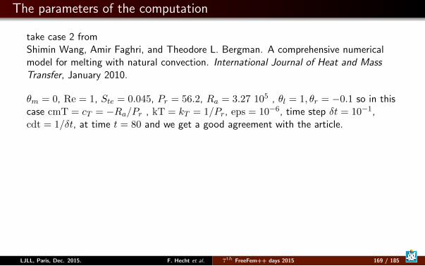
The parameters of the computation
take case 2 fromShimin Wang, Amir Faghri, and Theodore L. Bergman. A comprehensive numericalmodel for melting with natural convection. International Journal of Heat and MassTransfer, January 2010.
θm = 0, Re = 1, Ste = 0.045, Pr = 56.2, Ra = 3.27 105 , θl = 1, θr = −0.1 so in thiscase cmT = cT = −Ra/Pr , kT = kT = 1/Pr, eps = 10−6, time step δt = 10−1,cdt = 1/δt, at time t = 80 and we get a good agreement with the article.
LJLL, Paris, Dec. 2015. F. Hecht et al. 7th FreeFem++ days 2015 169 / 185
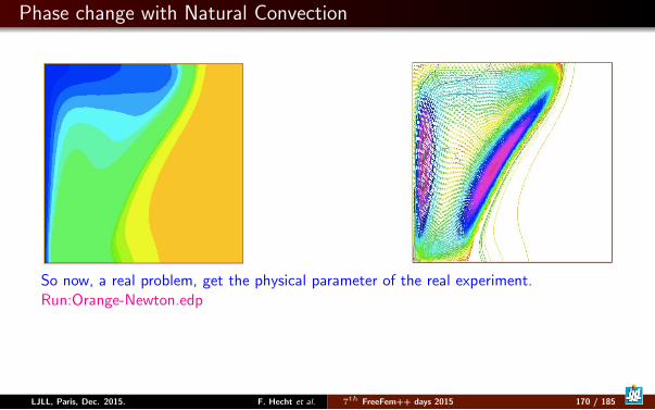
Phase change with Natural Convection
So now, a real problem, get the physical parameter of the real experiment.Run:Orange-Newton.edp
LJLL, Paris, Dec. 2015. F. Hecht et al. 7th FreeFem++ days 2015 170 / 185
Outline
1 Introduction
2 Tools
3 Academic Examples
4 Numerics Tools
5 Schwarz method with overlap
6 Exercices
7 No Linear Problem
8 Technical Remark on freefem++
LJLL, Paris, Dec. 2015. F. Hecht et al. 7th FreeFem++ days 2015 171 / 185

Outline
8 Technical Remark on freefem++compilation processPluginPlugin to read imagePlugin of link code through a pipeFreeFem++ et C++ type
LJLL, Paris, Dec. 2015. F. Hecht et al. 7th FreeFem++ days 2015 172 / 185
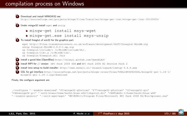
compilation process on Windows
1 Download and install MINGW32 seehttp://sourceforge.net/projects/mingw/files/Installer/mingw-get-inst/mingw-get-inst-20120426/
2 Under mingw32 install wget and unzip
mingw-get install msys-wgetmingw-get.exe install msys-unzip
3 To install freeglut of win32 for the graphics part
wget http://files.transmissionzero.co.uk/software/development/GLUT/freeglut-MinGW.zipunzip freeglut-MinGW-2.8.0-1.mp.zipcp freeglut/include/* /c/MinGW/include/GL/.cp freeglut/lib*.a /c/MinGW/lib/.cp freeglut/freeglut.dll /bin
4 install a good blas (OpenBlas) http://xianyi.github.com/OpenBLAS/
5 install MPI for // version HPC Pack 2008 SDK and HPC Pack 2008 R2 Service Pack 2
6 install inno setup to build installer: http://www.xs4all.nl/˜mlaan2/ispack/isetup-5.4.0.exe
7 GSL for gsl interface http://sourceforge.net/projects/mingw-cross/files/%5BLIB%5D%20GSL/mingw32-gsl-1.14-1/mingw32-gsl-1.14-1.zip/download
Finaly, the configure argument are:
./configure ’--enable-download’ ’FC=mingw32-gfortran’ ’F77=mingw32-gfortran’ ’CC=mingw32-gcc’’CXX=mingw32-g++’ ’-with-blas=/home/hecht/blas-x86/libgoto2.dll’ ’CXXFLAGS=-I/home/hecht/blas-x86’’--enable-generic’ ’--with-wget=wget’ ’MPIRUN=/c/Program Files/Microsoft HPC Pack 2008 R2/Bin/mpiexec.exe’
LJLL, Paris, Dec. 2015. F. Hecht et al. 7th FreeFem++ days 2015 173 / 185
Outline
8 Technical Remark on freefem++compilation processPluginPlugin to read imagePlugin of link code through a pipeFreeFem++ et C++ type
LJLL, Paris, Dec. 2015. F. Hecht et al. 7th FreeFem++ days 2015 174 / 185
Dynamics Load facility
Or How to add your C++ function in FreeFem++.First, like in cooking, the first true difficulty is how to use the kitchen.I suppose you can compile the first example for the examples++-load
numermac11:FH-Seville hecht# ff-c++ myppm2rnm.cpp...
add tools to read pgm image
LJLL, Paris, Dec. 2015. F. Hecht et al. 7th FreeFem++ days 2015 175 / 185
Outline
8 Technical Remark on freefem++compilation processPluginPlugin to read imagePlugin of link code through a pipeFreeFem++ et C++ type
LJLL, Paris, Dec. 2015. F. Hecht et al. 7th FreeFem++ days 2015 176 / 185
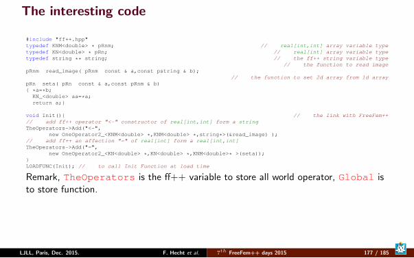
The interesting code
#include "ff++.hpp"typedef KNM<double> * pRnm; // real[int,int] array variable typetypedef KN<double> * pRn; // real[int] array variable typetypedef string ** string; // the ff++ string variable type
// the function to read imagepRnm read_image( pRnm const & a,const pstring & b);
// the function to set 2d array from 1d arraypRn seta( pRn const & a,const pRnm & b) *a=*b;
KN_<double> aa=*a;return a;
void Init() // the link with FreeFem++// add ff++ operator "<-" constructor of real[int,int] form a stringTheOperators->Add("<-",
new OneOperator2_<KNM<double> *,KNM<double> *,string*>(&read_image) );// add ff++ an affection "=" of real[int] form a real[int,int]TheOperators->Add("=",
new OneOperator2_<KN<double> *,KN<double> *,KNM<double>* >(seta));LOADFUNC(Init); // to call Init Function at load time
Remark, TheOperators is the ff++ variable to store all world operator, Global isto store function.
LJLL, Paris, Dec. 2015. F. Hecht et al. 7th FreeFem++ days 2015 177 / 185
Outline
8 Technical Remark on freefem++compilation processPluginPlugin to read imagePlugin of link code through a pipeFreeFem++ et C++ type
LJLL, Paris, Dec. 2015. F. Hecht et al. 7th FreeFem++ days 2015 178 / 185
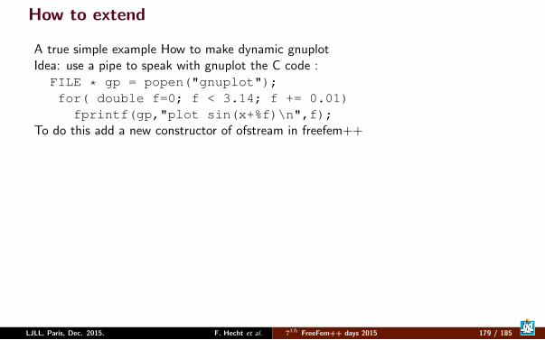
How to extend
A true simple example How to make dynamic gnuplotIdea: use a pipe to speak with gnuplot the C code :FILE * gp = popen("gnuplot");for( double f=0; f < 3.14; f += 0.01)fprintf(gp,"plot sin(x+%f)\n",f);
To do this add a new constructor of ofstream in freefem++
LJLL, Paris, Dec. 2015. F. Hecht et al. 7th FreeFem++ days 2015 179 / 185
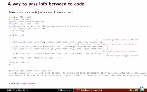
A way to pass info between to code
Make a pipe, under unix ( with a use of pstream tools )
#include "ff++.hpp"#include "pstream.h"typedef redi::pstream pstream;typedef std::string string;static pstream ** pstream_init(pstream **const & p,string * const & a) *p = new pstream(a->c_str());
return p;;
void inittt()
// add new pointer type * pstreamDcl_TypeandPtr<pstream*>(0,0,::InitializePtr<pstream*>,::DeletePtr<pstream*>);
// add cast operation to make std iostream read and writeatype<istream* >()->AddCast( new E_F1_funcT<istream*,pstream**>(UnRef<istream* >));atype<ostream* >()->AddCast( new E_F1_funcT<ostream*,pstream**>(UnRef<ostream* >));
// the constructor from a string .TheOperators->Add("<-",new OneOperator2_<pstream**,pstream**,string*>(pstream_init) );
// add new keyword type pstreamzzzfff->Add("pstream",atype< pstream ** >());
LOADFUNC(inittt);t
MBP-FH:plugin hecht$ ff-c++ pipe.cpp/usr/local/bin/g++ -c -g -m64 -fPIC -DNDEBUG -O3 -DBAMG_LONG_LONG -DNCHECKPTR -fPIC -I/usr/local/lib/ff++/3.20/include ’pipe.cpp’/usr/local/bin/g++ -bundle -undefined dynamic_lookup -g -m64 -fPIC -DNDEBUG -O3 -DBAMG_LONG_LONG -DNCHECKPTR -fPIC ’pipe.o’ -o pipe.dylib
a small test : Run:gnuplot.edp
LJLL, Paris, Dec. 2015. F. Hecht et al. 7th FreeFem++ days 2015 180 / 185
Outline
8 Technical Remark on freefem++compilation processPluginPlugin to read imagePlugin of link code through a pipeFreeFem++ et C++ type
LJLL, Paris, Dec. 2015. F. Hecht et al. 7th FreeFem++ days 2015 181 / 185
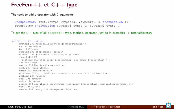
FreeFem++ et C++ type
The tools to add a operator with 2 arguments:
OneOperator2_<returntype ,typearg1 ,typearg2>(& thefunction ));returntype thefunction(typearg1 const &, typearg2 const &)
To get the C++ type of all freefem++ type, method, operator, just do in examples++-tutorialdirectory
c++filt -t < lestablesCmatrix 293 Matrice_Creuse<std::complex<double> >R3 293 Fem2D::R3bool 293 bool*complex 293 std::complex<double>*element 293 (anonymous namespace)::lgElementfunc 294 C_F0
ifstream 293 std::basic_istream<char, std::char_traits<char> >**int 293 long*matrix 293 Matrice_Creuse<double>mesh 293 Fem2D::Mesh**mesh3 293 Fem2D::Mesh3**ofstream 293 std::basic_ostream<char, std::char_traits<char> >**problem 294 Problemreal 293 double*solve 294 Solvestring 293 std::basic_string<char, std::char_traits<char>, std::allocator<char> >**varf 294 C_argsvertex 293 (anonymous namespace)::lgVertex
LJLL, Paris, Dec. 2015. F. Hecht et al. 7th FreeFem++ days 2015 182 / 185
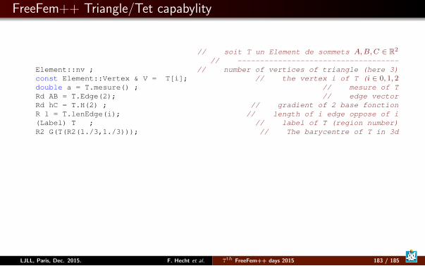
FreeFem++ Triangle/Tet capabylity
// soit T un Element de sommets A,B,C ∈ R2
// ------------------------------------Element::nv ; // number of vertices of triangle (here 3)const Element::Vertex & V = T[i]; // the vertex i of T (i ∈ 0, 1, 2double a = T.mesure() ; // mesure of TRd AB = T.Edge(2); // edge vectorRd hC = T.H(2) ; // gradient of 2 base fonctionR l = T.lenEdge(i); // length of i edge oppose of i(Label) T ; // label of T (region number)R2 G(T(R2(1./3,1./3))); // The barycentre of T in 3d
LJLL, Paris, Dec. 2015. F. Hecht et al. 7th FreeFem++ days 2015 183 / 185
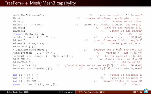
FreeFem++ Mesh/Mesh3 capabylity
Mesh Th("filename"); // read the mesh in "filename"Th.nt ; // number of element (triangle or tet)Th.nv ; // number of verticesTh.neb or Th.nbe ; // numbe rof border element (2d) or(3d)Th.area; // area of the domain (2d)Th.peri; // length of the bordertypedef Mesh::Rd Rd; // R2 or R3Mesh2::Element & K = Th[i]; // triangle i , int i∈ [0, nt[Rd A=K[0]; // coor of vertex 0 of triangle KRd G=K(R2(1./3,1./3)): // the barycentre de K.Rd DLambda[3];K.Gradlambda(DLambda); // compute the 3 ∇λKi for i = 0, 1, 2Mesh::Vertex & V = Th(j); // vertex j , int j∈ [0, nv[Mesh::BorderElement & BE=th.be(l) ; // border element l∈ [0, nbe[Rd B=BE[1]; // coord of vertex 1 on Seg BERd M=BE(0.5); // middle of BE.int j = Th(i,k); // global number of vertex k∈ [0, 3[ of tria. i∈ [0, nt[Mesh::Vertex & W=Th[i][k]; // vertex k∈ [0, 3[ of triangle i∈ [0, nt[
int ii = Th(K) ; // number of triangle Kint jj = Th(V) ; // number of triangle Vint ll = Th(BE) ; // number of Seg de bord BEassert( i == ii && j == jj) ; // check.
LJLL, Paris, Dec. 2015. F. Hecht et al. 7th FreeFem++ days 2015 184 / 185
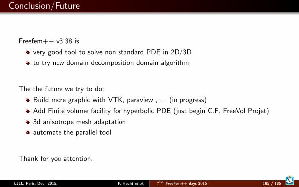
Conclusion/Future
Freefem++ v3.38 is
very good tool to solve non standard PDE in 2D/3D
to try new domain decomposition domain algorithm
The the future we try to do:
Build more graphic with VTK, paraview , ... (in progress)
Add Finite volume facility for hyperbolic PDE (just begin C.F. FreeVol Projet)
3d anisotrope mesh adaptation
automate the parallel tool
Thank for you attention.
LJLL, Paris, Dec. 2015. F. Hecht et al. 7th FreeFem++ days 2015 185 / 185