F. Calogero

SOME APPLICATIONS OF A CONVENIENT FINITE-DIMENSIONAL MATRIX REPRESENTATION OF THE DIFFERENTIAL OPERATOR

Summary. The matrices X and Z_, of order n , defined in terms of n arbitrary distinct numbers x. by the formulae X = diag(x), Z..- .2/ (x.—x.) if

j = k , Z.£ =(#. -A; , ) - 1 if j¥~- k , are representations of the multiplicative ope­rator x and of the differential operator d/dx , appropriately projected in the n-dimensional functional space of the polynomials in x of degree less than n . Various precise formulations and implications of this finding are exhibited, and several applications discussed.

Contents.

1. Introduction.

2. Finite-dimensional matrix representation of the differential operator.

2.1 Basic definitions and results. 2.2 Connection with Lagrangian interpolation. 2.3 Algebraic structure. 2.4 The algebra of raising and lowering operators: explicit realizations. 2.5. Finite-dimensional matrix representation of the differential operator for

periodic functions.

3. Explicit construction of remarkable matrices.

3:1 Matrices with known spectrum. 3.2 Matrices with known inverse. 3.3 Matrices satisfying "Lax equations" .

4. Deter-minantal representation of polynomials satisfying linear ODEs.

5! Detcrminantal representation of orthogonal polynomials.

6. Numerical evaluation of the eigenvalues of differential operators.

1980 Mathematics Subject Classification: 15-00, 15A24, 33A65, 65.D25, 65L15, 65N25

24

7. Envoi.

8 Refcrences.

1. Introduction.

In this paper we report a number of results; additional findings, as well as theproofs of those listed here, can be found in the papers referred to below. Section 2 contains the basic results; the following Sections, some applications.

Ali equations are numbered progressively within each section and sub­section; eq. (4) of subsection 2.1 is referred to as (4) within subsection 2.1 and as ¢2.1-4) elsewhere.

2. Finite-dimensional matrix representation of the differential operator.

2.1. - Basic definitions and results.

Throughout this paper « is a (fixed but arbitrary) positive integer;

lower case underlincd charactcrs are w-vectors, upper case underli-ned charactcrs are squarc matrices of ordcr n : thus the w:vector v

has the n components v. , the matrix M has the n2 clemcnts M.k , the w-vecto'r vo — Mv has the n components w.= 2 M, v, , the scalar

— — J k=i Jk k

n product ( w , £ ) = .2 u.v. , e t c . Unless otherwise spccified, indices run

from 1 to n . The n numbers x. are generally arbitrary (possibly complex), except

for the requirement that they be different,

( 1 ) x. ¥= xk if j ¥= k ;

only in some special cases we will consider specific choiccs of these n numbers.

The following vectors and matrices are defined in terms of the n

25

numbers X. :

(2) X = disig(xj)>Xjk=òjkx. ,

(3a) Jk J j=i J % J

<3b) zjk=(<xrxk^x i f i^k >

(4)

(5) B = diag(è.) , B.,= S. ,è . .

Here, and always below, a prime appended to a sum signifies omission of the singular term, and a prime appended to a product signifies omission of the vanishing factor.

Note incidentally that (3a) and (3b) imply

(3c) ì Z . =2z. , 2 2 = 0 .

The basic result can be formulated stating that the two matrices X resp. Z are representations of the (multiplicative) operator x resp. the differential operator d/dx , projected in the /^dimensionai functional space of the polynomials in x of degree less than n .

More precise formulations of this result can be expressed as follows [C1982c] [C1983c]:

Proposition 2.1.1: Let f(x) be an arbitrary polynomial of degree less than n ,

(6a) f(x)= "s* e x™ ,

and fr) (x) its rth-derivative,

(6b) fri (x) = drf(x)/dxr = n% [m\/(m-r)\]c xm-*>=0,1, 2,..., n-\ .

Let / resp. /*r) be the w-vectors whose components are the w values that f(x) resp. /^(tf) take at the w points *. :

(7) /J =/<*,•) , /<r) =/< f ) (*,) •

26

There holds then the following w-vector formula:

(8) fr) = BZr i"1 f •

For a derivation of this important formula, see the following subsection 2.2.

The following corollaries are immediate consequences of this result.

Corollary 2.1.2 •. The matrix Z is nilpotent,

(9) Zn = 0 .

Corollary 2.1.3 : Let,s/ be any differential operator,

(10) .<*= 2 a (x)dr/dxr ,

for which there holds the formula

(11) sff(x) = 0 ,

with f(x) a polynomial in x of degree less than n (see (6a)) . Define the matrix A , associated with the operator stf via the replacement x-* X. , dA/# -> Z :

(12) 4 = S a(X)Zr .

Then to the differential equation (11) there corresponds the w-vector formula:

(I3a) ^ £ = 0 ,

(I3b) l'^B-1 f .

Note that this generally also implies that the determinant of A vanishcs:

(14) det^4 = 0 .

Another formulation of the basic result reads as follows [CI98la] :

27

Proposition 2.1.4: To every choice of the n numbers x. (with (1)) there correspond weights w (x) and sets of n orthogonal polynomials q^]_x (x) , / = 1, 2, ..., n (generally ali of them of degree » — 1 ) , for which the following formulae hold:

(15a) fdx w (x) qn% (x) q^ (x) = òjk ,

(15b) fdx w (x) q^ (x) x q^ (x) = Xjk = bjk Xj ,

(15c) fdx w (x) q^ (x) (d/dx) q% (x) = Zjk ,

with

(15d) fflW = ^ - i W •

Let us indicate two explicit realizations of these formulae. Let p (x) be the polynomial of degree n that vanishes at the n

points x. ,

(16) P„<*)= n (*-*,•) .

and pljlx (x) be the n polynomials, of degree n- 1 , that obtain facto­ring away from p (x) one of its zeros:

(17) pf (x) = p (x)/(x-x)= Il .(x-x.) .

Note that these definitions imply the following formulae:

(18a) p^x{Xj) = p,n{Xj) = bj f

(18b) P^<*k) = ZjkPtì(xj) = Bjk .

(18c) dpì«\(x)/dx= £ p£\(x)Zkj

It is then easily seen that a (discrete) realization of (15) obtains as f ollows :

(19a) w(x)= ì 5 (a?-*.) ,

28

(19b) q^x (x) = q®x (x) =p^ <*)/£& (x.)

Another realization (or rather, a class of realizations) of(15)obtain as follows: let p (x) , m — 0, 1, 2, ..., n — 1 be n polynomials, each of degree m , that together with p (x) , see (16), and with an appropriate weight w (x) , constitute a set of n 4- 1 orthogonal polynomials:

(20) jdx w(x)pl (x)pm (x) = àlm , / = 0, 1, ..-.-,». ; ra = 0, 1, ..., w .

Then (15) hold with [C198ia]

(21) q^_l(x)=p{jll{x)=--pn{x)/(x-xj)

(for the expression of C2 , see eq. (2.8) of [C1981a]; note that we have assumed here that k = 1 , as implied by a comparison of (16) with eq. (1.1) of [C1981a]; this can always be.achieved by rescaling w (x) , to satisfy (20) with / = m — n ) .

Let us end this subsection reporting the explicit expression of the matrix Z2 :

(22a) (Z2) =z2 - I ' (x-x.)~2=Ì 2 (x.-x.)'1 (x. -x T1 if j = k ,

(22b) (Z2)., = 2 ( * - ^ ) - ^ ^ ^ if j±k .

2.2. - Connection with Lagrangian interpolation.

The connection [C1982c]of the results reported in the preceding subsec­tion 2.1 with the classical proolem of Lagrangian interpolation is clear; indeed the polynomials (2.1-19b) are precisely the Lagrangian interpolational polyno­mials associated with the n points x. . In this subsection we report some of the relevant formulae.

Let F (x) be a real function defined in the real interval xL < x < xv , and let the n (different, real) points x. fall in that interval, say

(1) xL <xl <x2 < ... <x <x

29

Let f. indicate the n values that the function F (x) takes at the n points x. :

(2) F(x.)=f...

Let f(x) be the (unique) poiynomial of degreeless than n that takes the n values / . at the n points x. -.

(3a) / ( * ) = "s1 e xm ,

(3b) / ( * , • ) = / • •

There hold then the formulae (Lagrangian interpolation)

(4a) f^)=ìjjp^_1{x)/pf_l(xj) ,

(4b> /W=(IM , r1/).

(5) F(x)=f(x)+pn(x)F{n)[x(x)]/n\,xL<x(x)<xu .

In (4) we have used the notation defined by (3b) (see also (2.1.-7) and (2.1.-16, 17, 18, 5)) , and we have introduced the w-vector ir {x) of components

(6) n

ir. (x)~pv> (x) = p (x)/(x — x.)= Il (x — x.)'\

this formula, (4), defines the poiynomial f(x) that interpolates the function F (x) at the n points x. . Note that the important formula (2.1.-8) obtains differentiating (4b) r times, using the identity (see(2.1.-18c))

(7) dii(x)/dx = ZT 2(X) = TÌ(X)Z ,

then setting x = x. , j = 1, 2, ..., n , and using (2.1.- 18b) The formula (5) serves to assess to what extent the poiynomial f(x)

approximates F (x) at x^x. ; F(n)(x) indicatés of course the n — th derivative of F (x) , evaluated at some appropriate point x (depending on x , as indicated in (5); of course in an unknown fashion; but surely falling, as indicated in (5), within the interval (xL , #^)) . There also holds

30

an analogous formula fC1983c] for the derivatives of F (x) :

(8) drF(x)/dxr=drf(x)/dxr +

+drp (x)/dxr F^n)\x(x,r)]/n\ , xL <x~(x , r) <xy , r = 1, 2, ..., n

(of course^* , n)-x , since dn f(x)ldxn =0 , see (3a), and dnpn (x)/dxn = n\ , see (2.1.-16)).

In this connection let us also record the formula (see (7))

(9) drpn(x)/dxr= . 2 ^ ^ ( ^ ) ( ^ ^ ^ , ^ = 1 , 2 , 3 , . . . ,

implying

(10a) p'n (*) = £. (see(2.1.-18a)) ,

(10b) //'<*.) = 2*. z. (see (2.1.-30) .

2.3 - Algebraic structure.

The basic rcsult of subsection 2.1 could also be obtained by a purely algebraic approach. The ma in formulae of this approach read as follows [C1980c], [C1980b], [C1981al, [C1981bj, [C1983a]:

(1) lZ,X]=L-J=l-nP ',

(3) Jjk = 1 ' P j k = ì/n'?2=?>JZ = ° >

(4) ^ w j = ^ M - 1 / ^ J m = l , 2 , ...,w (see (2,1.-4)) ,

<5a) jv(™)=Pv(m)=0 , ro = 1,2, . . . , » - 1 ,

(5b) Jv(n)=u , «. = 1 ,

(6) Xv<m)=y!m + 1) , m = l, 2 , . . . , « - l ,

(7) 2 : ^ = ( ^ - 1 ) ^ - 1 ) , m = l , 2 , ...,» .

31

Note that (6) does not hold for m = n (indeed v_(n +1) is not defined, while X rfn) is generally some combination of the n vectors v^n) , see (4), with coefficients depending on the x's) ; while (7) holds for ali the n values m = 1, 2, ..., n . These formulae, (6) and (7), correspond aigebraically to the relation x^-X , d/dx-+Z_ , via their analogy with the trivial equa-tions

(8a) <p(m) (x) = xm~1 , m = l , 2, 3, ...,

(8b) xy(m) (x) = v(m + 1) (x) , fw= 1,2,3,...,

(8c) d<p(m) (x)/dx = (m-ì)^(m-1) (x) , m = \, 2, 3,• ..., .

The fact that (7) holds for m = l , 2 , ..., n while (6) holds only for m = l , 2, ..., n — 1 corresponds to the fact that the differential operator d/dx , when acting in the functional space spanned by the polinomials of degree less than n (where a basis is provided by the first n monomials \pim) (x), m = 1, 2, ..., n , see (8a)) remains within this space, while the multiplicative operator x stays within this space only when acting on (p<m ) (x) with m < n ; a counterpart of this fact is the difference between the commutation rule (1), and its counterpart

(9) [d/dx ,x]=l .

It is also of interest to introduce the set of vectors u(m) orthonormal to the z/w *' s . They are defined as follows. Let

(10) p (x)= lì (x-x.)= 2 . a xm , a = 1

Then

(Ila) u(m)= ì a Xr~m u , m = l ,2 , ..., » ,

( l lb) u(n) =u , z/. = l

There hold then the following formulae:

(12) (u(l) ,v!m)) = òl m

32

(13a) V.. =v<k)=xk-1/ II' (x.-x ) ,

(13b) ^ = « ^ = S . " » ^ .

(13c) ^ = 1 ^ = 1 >

(13.d) det V= fì ( a r . - * . ) - 1

(13e) det U= lì (x.-xk) n n

- j>k=i J

(14a) z / m ; Z = ZT u(m) = mu<m + l), m = 1,2, . . . , » - 1 ,

(14b) u(n) Z = ZT u(n) =uZ = 0 ,

(15) « r m ; X = ^ « r m ; = « w " 1 - « w _ i « >

(16) ^ D y * = i V i .

(17a) ( ^ D ; f e= 6

; > + i » / = 1 , 2 , . . . , » ; * = 1 , 2 , . . . , » - 1 ,

(17b) ( ^ ) , - , = - ^ 1 , / = 1 , 2 » .

It is also of interest to display some formulae invoiving the matrix

(18a) N = XZ ,

(18b) N.=x.z.= x. £' (x.-xT1 if / = £ , } K s i J ì =i\ J *

(18c) Njk=xj{x.-xkr1 \i j*k .

They read:

(19) ÌV£ ( W )=(W-1)£ ( W ) ,

(20) u(m) N =NT u(m)=(m-l)u(m) ,

(21) t / W = diagO'-D ,

33

Note that this matrix has the first nonnegative integers as its eigenvalues; this corresponds (see Corollary 2.13) to the formulae

(22) [xd/dx-(m-l)]ip(m) (x) = 0 , m = l, 2, ...,

with p<m) (x) defined by (8a). The isospectrality of the matrix N (x) , namely the fact that its

eigenvalues do not depend on the vector x that defines its matrix elements, see (18), can also be displayed by exhibiting the following formulae:

(23) N(y)=W(y,x)N(x)[W(y , * ) ] - 1 ,

(24a) W (y, x) = V (y) U (x) ,

(24b) Wjk(y,x) J m =£;

(24c) [WC^,*)]"1 = E (*,X) ,

(24d) W(* ,y ) W ( ^ , z ) = W(x, z) »

(24e) W ( * , * ) = I >

(25a) òN/òx, = [M(i} , N] ,

yj xj A y> xm yrxk zV;yi~y>»

(25b) M(™}=Z .(8. - 5 . . ) ,

(26a) N=[M,N] ,

(26b) M=VU = -VÙ = XZ- diag <*Z)

In the last formulae the dot indicates differentiation with respect to a variable t on which the numbers x. may (arbitrarily) depend; note that (26a) has the form of a "Lax equation", but it is of course an identity (with (26b)), without any "dynamical" content.

34

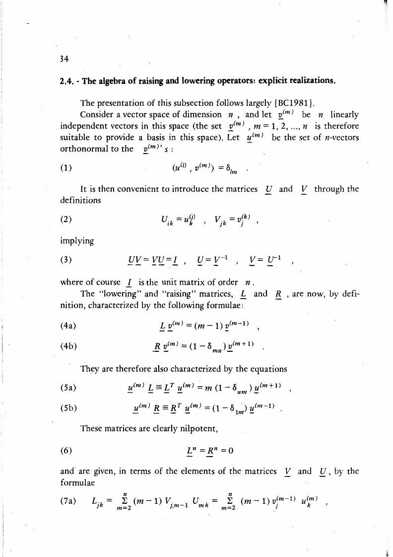
2.4. - The algebra of raising and lowering operators: explicit realizations.

The presentation of this subsection follows largely [BC1981]. Consider a vector space of dimension n , and let i/m* be n linearly

independent vectors in this space (the set vjm) , w = l , 2 , . . . , w is therefore suitable to provide a basis in this space). Let t£(m) be the set of 72-vectors orthonormal to the vfm)' s :

(1) («'»,*<""> =5 / w .

It is then convenient to introduce the matrices U and V through the definitions

implying

(3) uv=Yu=L > ¥=Y~1 > Y= LT1 >

where of course _/ is the unit matrix of order n . The "lowering" and "raising" matrices, L^ and R , are now, by defi-

nition, characterized by the foliowing formulae:

(4a) Ltfm)=(m-\)v<m-l) ,

(4b) Rv(m) =(1-8 ) v( m + 1) .

Théy are therefore also characterized by the equations

(5a) u(m) L = LT u(rn) =m(l-6 )u(m + iy ,

(5b) u(m) R = RT u(m) = ( 1 - 5 ^ ) . ^ - ^ •

These matrices are clearly nilpotent,

(6) Ln=Rn=0

and are given, in terms of the elements of the matrices V and U, by the formulae

n n (m-1) ll(m) (7a) L. = 2 (m-l)V. t U . = 2 (m~\)v{m-l) u{T

35

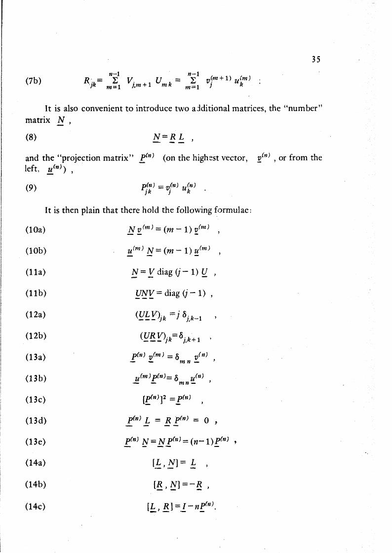
<7b> v=3ì V M ^ - J I °<rl)<m) • It is also convenient to introduce two additional matrices, the "number"

matrix N ,

8) N = R L ,

and the "projection matrix" P(n) (on the highsst vector, v(n) , or from the eft, ujn)) ,

9) Pf*> = vjn) u(kn) .

It is then plain that there hold the following formulae :

IOa) Nv(m) = (m-l)v(m) ,

lOb) u{m) N=(m-l)u(m) ,

I la) N = y d i a g ( / - 1 ) U ,

l lb) UNV=dmg(j-l) ,

12a) (ykY)jk=J8jtk-i >

13a) Pr"; z/m; =5 z/"; ,

13b) a ^ P ^ = 5 arw) ,

13c) [P(n)]2 = PM ,

13d) Pf"> L = RP(n} = 0 ,

13e) l(n) N = NP(n) = (n-l)P(n) >

14a) [ ^ , ^ 1 = ^ .

14b) [R,N]=-R ,

14c) [L, #]==/-wP r" ; .

36

The following results are also plain.

Proposition 2.4.1: The matrix

(15a) M(L) =N+ 2 "X c^LiJSP

has the same eigenvalues as the matrix N , namely the first n nonnegative integers:

(15b) [M(L) -{m- 1)] [z/m; 4-^S1 a{m) v(s)/(s - 1)!] = 0 . s=l

Here the coefficients e are arbitrary (except for the requirement oo ' ' • .

that 2 ( w - l f c converge), and the coefficients a[m) are deter­g o Pi b s

mined recursively according to the formula

(15c) (m~s)a(sm) =(m-l)l 2 e tyn-\? +

m~\ p=0 P<n'-S

+ 2 ^ m ; 2 V ( r - i y , s = m - l , m - 2 , ..., 1 .

(Here, and always below, by convention a sum vanishes if the lower limit exceeds the upper limit).

Proposition 2.4.2: The matrix

oo W—1

(lóa) M(I<)=N+ 2 2 e R<* N?

has the same eigenvalues as the matrix N , namely the first n nonnegative integers :

(I6b) [M(R) -(m-l)][v(m) + 2 h(m)v(s)] = 0. .*=m-fl "*"

Here the coefficients e are arbitrary (except for the requirement oo r '

that 2 (n—Vf e converge), and the coefficients b(m) are deter­g o Pi b s

37

mined recursively according to the formula

(lóc) (m - s) b<»> = 2 {m-lf e, _ + P=o P>s~m

s-\ + X b[m) 2c„ _Ar-\f, 5 = m + l,f» + 2,...,w .

Proposition 2.4.2: The eigenvalues JU of the generalized eigenvalue equation

(17a) M(1) (d)v^ (d) = nM(2)(d)vW (0)

are independent of 6 , if the two matrices A^1^ (0) and Af(2) (0) are defined by the formula

(17b) M(s) (0)= 1 ^ 1 ¾ 1 c^exp [ i ( r - $ ) 0 ] L * flr N? , s = l , 2. p=0 ^=0 r=0 — ~ —

Here the coefficients c(J} are independent of 0 , but otherwise arbitrary (except for the requirement that 2 cs)

r (n-\)p converge).

Ali these results are quite standard; and an explicit (trivial) representa-tion of the "lowering" and "raising" matrices, say L(T) and R(T) , is pro-vided by the formulae

jk J j.k-i ' jk j,k+1 '

implying

(18b) N(T) =R(T) L(T) = diag (; - 1) ,

(18c) u<T) = y<T)=lf

(18d) P[n)(r)=8. 5.

Ali other representations can be obtained from this via a similarity tran-sformation (see (11) and (12)). But the point to be emphasized here is the possibility to exhibit quite explicit representations of "lowering" and "raising" matrices, using the results of the precéding subsections.

One such representation is provided by the formulae

(19a) L = Z ,

38

(19b) £=;*(£"i;w;> >

with Z^ and X defined by (2.1.-3) and (2.1.-2) in terms of the n arbitra-ry numbers x. (ali different; see (2.1.-1)), and

(19c) P(^=xtl~x/bj (see (2.1.-4)) ;

since indeed, with these definitions (and with JJ and V defined in terms of x_ by (2.3.13)), the formulae of this subsection coincide with the corre-sponding formulae of the preceding subsection 2.3 (note that (8), (13d) and (19)imply (2.3-18a)).

It may be worthwhile to report explicitly the value that the matrices Z, and R_ take for the special choice

(20a) x. = exp (2irij/n) ,

implying (see (2.1.-16))

(20b) > , ( * ) = * " - 1 ,

and therefore (see (2.1.-18a) and (20a))

(20c) b. = n x?"1 =n/x. , ì l i

Theyread[C1981a]

(21a) Ljk=Z.k = - ( » - l ) / * . if / = * ,

i (21b) Lj^Z.^(x-xkT

1^--exp[-m(j+k)/n]/sin[Tr(j--k)/n] if ji^k,

(22a) R=X(I-J/n) ,

(22b) Rjk = x.(n-l)/n if / = * ,

(22c) Rjk=-x/n if j*k ,

(23a) Njk= i . ( , , -1 ) if j = k ,

(23b) N-k=~ ~ exp [m (j-k)/n]/sin [ir (j-k)/n] if /=É& .

39

Other explicit representations may be constructed as follows (we provide here a specific example; it should be clear how this can be generalized, see also section 5 below). It is well known that the Hermite polynomials H (x) have the following properties [SI939 ]:

(24a) ì ~ Hm_1(x) = (m-l)Hnt_1(x) , .»1 = 1,2,3,...,

(24b) \2x- -^J Hm_ì(x) = Hm(x) , w = l, 2, 3, ....,

/ d 1 d2\ ( 2 4 c ) ( # - — IH Ax)={m-\)H Ax) , m = 1,2,3, ... .

\ dx 2 dx2' m _ 1 w _ 1

The following formulae are therefore direct consequences of Corollary 2.1.3:

(25a) - Zi/H)(m) =(m-l)v(H)(m-1) ,m = l,2, ...,n ,

(25b) (2X-Z)v(H)(m)=i/H)(m + 1),m = l,2,...,n-l ,

(25c) (2)£-Z)v(H)(n) =Hn (X)v ,

(25d) (XZ- - Z2)lH)(m)=(m-\)T/H)(m) ,m = \,2,...,n ,

with

(25e) ^H)(m)=Hm_1{X)v , w = l , 2, . . . , » ,

(25f) v.= l/b. = l/ U' (x.-xb) .

It is then clear that, provided the n numbers x. are chosen to coin­cide with the n zeros of the Hermite polynomial of order n ,

(26a) H (*.) = 0 ,

so that the r.h.s. of (25c) vanishes, it is consistent to define the following "lowering" and "raising" matrices:

(27a) L(H) = - Z , - 2 —

40

(28) R(H) = 2X-£ .

Since the n zeros x. of the Hermite polynomial of order n are also characterized by the n algebraic equations [SI939]

(26b) XÌ=ZÌ= & (*>-xkT' >

the explicit expressions of the matrices L(H) and R(H) intermsof these numbers read

(27b) Lfk}= ~ x. if j = k ,

{Ile) L(»>= - (xj-xky1 if ji=k ,

(28b) Rjk)=xj i f J = k >

(28c) Rj»> =-(xj-xkT1 if j*k .

2.5. - Finite-dimensional matrix representation of the differential operator for periodic functions.

In this subsection we introduce, following[C1984a],results analogous to those of subsection 2.1, but applicable to periodic (or antiperiodic) functions. Let us also mention that there also exists another convenient representation of the differential operator applicable to periodic functions, which is actually neater than that discussed here-, we refer for this very recent development to the literature [C1984d], [CF1984].

The main finding is the matrix j£ defined, in terms of n arbitrary numbers x. different mod (L),

(1) x. =£xk mod (L) ,

by the formula

(2a) ^ = ( ^ ) P cotg[ir (* . -* . ) / ! ] if j = k ,

41

(2b) Zjk=(n/L)cotg[ir(xj-xk)/L] if )<* k .

This matrix, together with the matrix X , see (2.1.-2), yields, via the follo-wing Proposition, a finite-dimensional matrix representation of the differen-tial operator d/dx and of the multiplicative operator x , applicable, for even n , in the linear space of periodic functions of degree n (see below), and for odd n , in the linear space of antiperiodic functions of degree n (see below).

Proposition 2.5.1: If for a differential opera tore .

(3) s/ = 2 a (x)dr/dxr , »=o r

there holds the equation

(4) j * / ( * ) = 0

with f(x) either "a periodic function of even degree n — 2m^ , namely

(5a) 'f(x) = cl+c sin [nir (x-x)/L] +

:2s sin [2s7T (x -x)/L] + c2s+1 + 2 {c0v sin [2s7r (JC -#) /L] + c9c+1 cos [2s7r (# — x)/L]} , s = l

or "an antiperiodic function of odcl degree n = 2m 4- 1" , namely

(5b) f(x) = c cos [nir (x-x)/L] 4-m _

4- 2 {c2s sin [ (2s- l )7r (*-*) /£] 4 - ^ ^ cos[(2s-l)7r(^-^)/L]}

then for the matrix A_ (of order n ) ,

(6a) ^4 = 2 [a2<? (X) 4- « x (X) Z] [Z2 - (rnr/L)2 Pp ,

there holds the corresponding w-vector formula

(7) Aw = 0

42

with

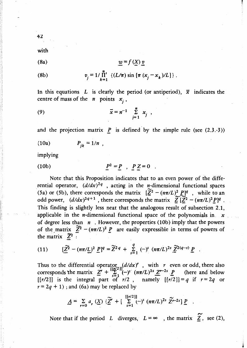
(8a) w=f(X)v

(8b) v. = l/flf {(L/ir) sin [ir (x.-xb)/L]} . J k=i * K

In this equations L is clearly the period (or antiperiod), x indicates the centre of mass of the n points x.,

(9) x = n 1 2 x. , ; - i '

and the projection matrix P is defined by the simple mie (see (2.3.-3))

(IOa) Pjk = Un ,

implying

(lOb) P2 = P , PZ = 0 .

Note that this Proposition indicates that to an even power of the diffe-rential operator, {d/dx)2q , acting in the w-dimensional functional spaces (5a) or (5b), there corresponds the matrix [Z2 - (nir/L)2 P\q , while to an odd power, (d/dx)2q + l , there corresponds the matrix Z [Z2 - {nit/L)2P]q . This finding is slightly less neat that the analogous result of subsection 2.1, àpplicable in the w-dimensional functional space of the polynomials in x of degree less than n . However, the properties (lOb) imply that the powers of the matrix Z^ -(nir/L)2 P are easily expressible in terms of powers of the matrix 2 2 :

(11) [Z2 -(nir/L)2 Pf=Z2q + Z (~)s (nir/L)2s Z2(q~s) P .

Thus to the differential operator (d/dx)r , with r even or odd, there also corresponds the matrix Zr + £ (-)5 (nir/L)2s ZT2s P (here and below [[r/2]] is the integrai part of r/2 , namely [[r/2]] = q if r=2q or r = 2q + 1) ; and (6a) may be replaced by

Ur/2U , ^ A = 2 a (X) { / + [ S H s (nir/L)2s Z^2s] P .

r=0 r s= l ""

Note that if the period L diverges, L = °° , the matrix Z , see (2),

43

goes into the matrix Z , see (2.1.-3), and the results of this subsection repro­duce those of subsection 2.1.

Since the value of L can be modified ad libitum by appropriately rescaling the variable x as well as the parameters x. , letus hereafter assu­me that

(12) L=TT

(note that we make this, notationally more convenient, assumption, rather than the more naturai one, L =? 27T ) . Then the matrix Z is defined by the neat formula

(13a) ^ * = J i c<*g <*>-*,•> if / = * >

(13b) Zjk=cotg(xj-xk) if j*k ,

with

(14) x. =£ xk mod (TT) .

It would be^easy to derive from Proposition 2.5.1 the spectrum and eigenvectors of Z and of Z2 — n2P (hint: let sé = - id/dx — v, / (x) = = exp(2Vjc) ,^=-(w-2) ,~(w-4) , . . . , (w-4) , («-2) , and sé = -d2/dx2 -v2 , / ( # ) = exp (± i- p # ) , p = » , w — 2 , » — 4 , ..., 1 or 0 ) ; but these results can also be obtained, more directly, in the following manner, that relates the findings of this subsection to those pf previous subsections. Define first of ali the matrix H,

(15) H=iZ ,

(15b) H..=i £ ' cotg (*.-*•> if j = k ,

(1 5 c) Hjk =i cotg (x.-xk) if /=££ ,

and then note that

(16) H = J + (n-2)l-2N

with the matrices J and / defined by (2.3.-3) and (2.3.-2), and the matrix N defined by (2.3.-18) but with x. replaced by x. .

(17a) x.• = exp (2i: x ) ,

44

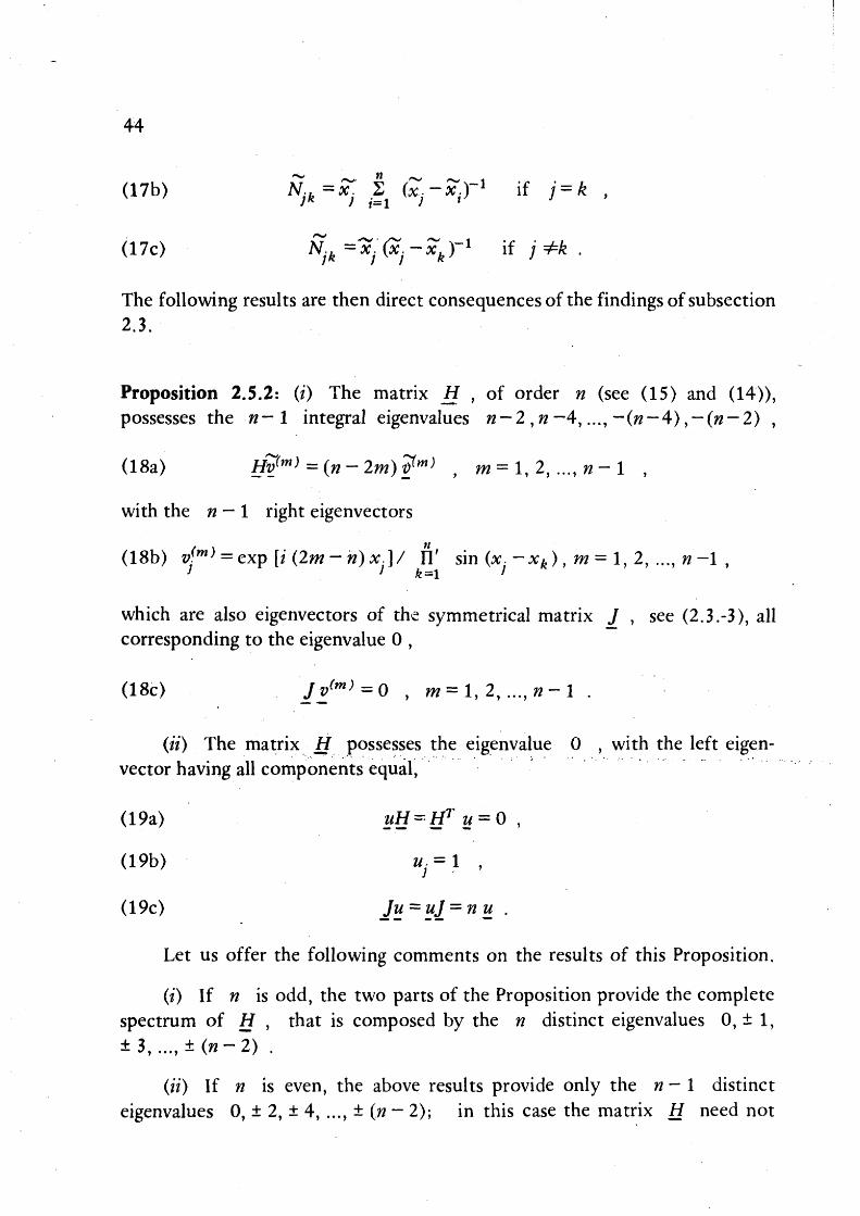
(17b) NJk=x. .2 (^ . -^ . ) - 1 if j = k ,

(17c) / ^ = ^ . ( ^ . - ¾ ) - 1 if ji=k .

The following results are then direct consequences of the findings of subsection 2.3.

Proposition 2.5.2: (i) The matrix H , of order n (see (15) and (14)), possesses the n— 1 integrai eigenvalues n — 2 ,n-4 , . . . , — (» — 4 ) , - ( « — 2) ,

(18a) Hv(m) =(n-2m)?m) , ra = 1, 2, . . . , /*-1 ,

with the /2 — 1 right eigenvectors

(18b) z/m; = exp [ i ( 2 m - w ) ^ . ] / Il' sin (x. -xk), m = 1, 2, ..., w -1 ,

which are also eigenvectors of the symmetrical matrix / , see (2.3.-3), ali corresponding to the eigenvalue 0 ,

(18c) Jv(m)=0 , m = l , 2 , . . . , w - l .

(ii) The matrix H possesses the eigenvalue 0 , with the left eigen-vector having ali componente equal,

(19a) uH = Hr u = 0 ,

(19b) u. = \ ,

(19c) Ju = uJ = n u .

Let us offer the following comments on the results of this Proposition.

(/') If n is odd, the two parts of the Proposition provide the complete spectrum of H , that is composed by the n distinct eigenvalues 0, ± 1, ±3 , . . . ,±( /2-2) .

(ii) If n is even, the above results provide only the n - 1 distinct eigenvalues 0, ± 2, ± 4, ..., ± (n - 2); in this case the matrix H need not

45

be diagonalizable, as displayed by the case n = 2 ,

(20) H = cotg(xì -x2) ( J .

However, if H is diagonalizable, these eigenvalues, with the vanishing eigen-value beiiig doublé, provide the complete spectrum of H, sirice their sum clearly vanishes and the definition (15) of H implies that its trace vanishes,

(21) t r H = 0 .

(iti) The spectrum of H is independent of the values of the n quan-tities x. ; thus this matrix provides one more neat example of isospectral matrix. A paradoxical aspect of this finding obtains setting x. = e y. and then letting e -• 0 ; the definition (15)of H would then seem to suggest that ali the eigenvalues of H should diverge proportionally to e - 1 , rather than remain Constant. The escape from the paradox originates of course from the fact that, as e -* 0 , H-> i e - 1 Z , see (2.1.-3), with the matrix Z being nilpotent, see (2.1.-9).

(tv) The definitions (2.3-3) of / and (15) of H imply the matrix formula

(22) JH=0 ,

which is clearly consistent with the simultaneous validity of (18a) and (18c).

(v) In the special case when the n points x. fili evenly the interval (0 , 7r) (mod (ir) ; and up to permutations), say

(23) x•~x1 + ( / - l )7 r /w ,

the matrix H becomes hermitian:

(23b) Hjk=0 if j*k ,

(23c) H.k =H*j = icotg[(j-k)Tt/n] if ji=k .

In this case H is of course diagonalizable (for n— 2 , it vanishes identically-, see (20)). The results for this special case were already known (see [CI979]

46

and section 4.1 of [C1981a]) .

(vi) Clearly other results can be inferred from those of subsection 2.3 via (16) with (17). This is left as an exercise for the diligent reader.

(vii) In an analogous manner it is easily seen that the matrix H2 + n2P, see (15) and (IOa), possesses the eigenvalues w2, (n — 2)2 , (n - 4 ) 2 , ..., 1 or 0 , ali of them doublé except the first, n2 , and (if n is even) the last, which are single-, note that the number of these eigenvalues is n (provided of course one counts twice the doublé eigenvalues), both for n even and for n odd.

3. - Explicit constructioiì of remarkable matrices -

In this section we outline one of the applications of the results given in the preceding section, namely the possibility to construct explicitly and easily remarkable matrices having known spectrum or inverse or satisfying "Lax type" equations. These findings may be useful to teach, or to test computer programs (to diagonalize or invert matrices).

The main idea to derive such matrices is to exploit the possibility, implied by the results of the previous section, to transform any differential equation valid for polynomials, in a corresponding formula valid in an w-di-mensional vector space and involving the matrices X and Z , see (2.1.-2) and (2.1.-3).

3.1. - Matrices with known spectrum.

The presentation here is limited to reporting some examples, which should suffice to convey the main idea; many additional explicit results are displayed in [C1981a], Moreover, see section 5 below.

The prototypical matrix having a known spectrum is the matrix N,

(la) W = X Z ,

db) Nik=xi 2' (x.-xf1 if j = k , JK ] i=i J l J

(le) ^-* = *y (*/"** T1 if j*k ,

47

(see subsection 2,3, in particular (2.3-18) and (2.3.-19)); and let us reemphasi-ze that the property of this matrix, to have the first n nonnegative integers as eigenvalues, is independent of the n parameters x. .

As implied by the results of subsection 2.4, a more general matrix ha-ving the same property is given by the explicit formula

(2) M(L)=N + f "z e Z« N? , — - p=0 q=l P4 - -

where the coefficients e are also arbitrary (see Proposition 2.4.1 and (2.4.-19a)). A special case or this matrix is

(3) N(H) =N- - Z2

(see (2.4.-21d>). Another matrix having the same spectrum is of course

(4) C_=(n-l)l-N(H) =(n-\)I+ - Z2 -XZ ,

indeed

(5) Cv(H)(m)=(n-m)v(H)(m) , m = 1, 2, ..., n,

with v(H)(m) defined by (2.4.-25e, 25f). On the other hand it is easily seen, using (2.1.-22), that

(6) £=è+£

with

(7a) Ajk= ì' (x -Xir2 if j = k ,

(7b) Ajk=~(xj-xky2 if j*k ,

(8a) Ejk= l^ y^Xj-x.)-1 if j = k ,

<8b) Ejk=yj(xj-xkr1 if ; ^ ^ ,

n _ 1

(8c) y. = - ^ . 4- 2. = — x. 4- 2 (A;.—je.) 1 .

It is therefore immediately concluded that the matrix A defined by the

48

neat formula (7) has the first n nonnegative integers as eigenvalues provided the n numbers x. are the n zeros of the Hermite polynomiàl of order n,

(9a) H (#.) = 0 ,

sincethen [S1939]

<9b) n ' - 1

X- 2J IX. Xt)

and therefore the matrix E in the r.h.s. of (6) vanishes identically (see (8)). Note that the property (9b) characterizes the n zeros of the Hermite

polynomiàl of order n ; this is not the case for the requirement that the matrix A , see (7), have the first n nonnegative integers as its eigenvalues [C1982b].

The fact that the matrix A , see (7), constructed with the n zeros of the Hermite polynomiàl of order n , has the first n nonnegative integers as its eigenvalues, was found (as a by-product of the study of certain integrable dynamical systems) in [C1978], vvhere analogous results for the other classi-cai polynomials are moreover given (see also [C1977], [ABCOP1979], [C1983a]). In the limit as n-*<*> , these findings go over imo results for singular integrai operators [CP1978], [C1979a] ,[C1979b], [A1980].

Finally let us point to the results of subsection 2.5 (see, for instance, Proposition 2.5.2) and of Ref. [C1984d], as one additional source of matrices with known spectrum.

3.2 - Matrices with known inverse.

In this subsection we merely cali attention to the (nontrivial) formula

(1) Wjk = [(y. -Xj)/<y. - * , ) ] ^n [(y.-xm )l(yj -ym )] ,

(2) <rJ>,* = [ (* , -> , )«*!~y k ) l ,n i [ (* ; - y m ) / ( X j -x m ) ] ,

implied by (2.3.- 24b, 24c); here the In numbers x., y. are arbitrary (possibly complex), except for the requirement that they ali be different.

I

49

3.3.- Matrices satisfying "Lax equations".

In this subsection we merely cali attention to the identity (2.3.- 26), implying the possibility to construct matrices that satisfy identically Lax-type equations, namely matrix equations of the form

(1) 1=1½. di •

Indeed clearly an equation of this type can readily be obtained for any isospe­ctral matrix L_ , namely any matrix whose elements depend on some parame-ter t (and the dot in (1) indicates of course partial differentiation with respect to t ) while its spectrum is Mndependent; indeed it can be easily shown that (1) is sufficient and necessary (with some appropriate matrix A ; which is clearly not unique) in order that L (t) be isospectral. And the results of the preceding subsections (see, in particular, subsection 3.1) indica­te how a large crop of such matrices can be readily exhibited.

Starting from a Lax equation that holds identically, it is easy to manufa-cture a Lax matrix that satisfies (1) only if some dynamical equations are sati-sfied. Indeed, as an immediate consequence of (2.3.- 26), it is seen that (1) holds with

(2a) Ljk=xj J j (x.-x.T1 if / = * ,

(2b) Ljk = x. (x. -xkT1 if j*k ,

(3a) A.k=- t[ y^x.-x.)-1 if ; = * ,

(3b) Ajk=~ y^xrxk^1 if i*k.'

if the x(t)'s "evolve" according to the "dynamical equation"

(4) À(t)=y[x_(t) ,t] .

Here we assume the n components y. (x, t) to be given (arbitrary) fun-ctions of the w-vector x and of t ; and of course the fact that (4) implies (1) via (2) and (3) does not imply that the dynamical system (4) is completely integrable (the n eigenvalues of .L do provide in this case n constants of the motion in involution; but rather than functions of the x. 's , these n constants are merely the first n nonnegative integers, hence their constancy has no dynamical relevance,whatsoever).

50

4.- Determinantal representation of polynomials satisfying linear ODEs.

The main finding [C1984b] is embodied in*the following

Proposition 4.1: For any polynomial P (x) of degree m <w that sati-sfies the linear ODE

m

(1) s4P (x) = 2 a (x)drP (x)/dxr = 0 ,

there holds the formula (2) P (#)Q (x) = det [A'+ XA -xA] ,

with Q _w (#) a polynomial of degree n~m and the matrices X.,A and A' , of order /z, defined as follows:

(3) X = diag(*.) (see(2.1.-2)) ,

(4a) Zjk= r (Xj-x.T1 if j = k (see.(2.1.-3a)) ,

<4b) ' Zjk ={xj-xkT1 ii j = k (see(2.1.-3b)) ,

w

(6) ^ ' = S r a (X)Z- 1 ,

in terms of the n arbitrary distinct numbers x- . The proof of this Proposition is quite simple. Let y be a zero of P (x) ,

and define the polynomial Pm_1(x) , of degree m — 1 , by the formula

(7) Pw_ t W = Pm (*)/<* - y ) . .

It is then easily seen that (1) implies the equation

(8) W +x.sé-ysé\Pm_x (*) = (>,

withcc/ defined by (1) and s/' defined by the formula

m (9) s/'= 2 ra (x) dr~x /dxr~l

r=l r

51

There follows, using Corollary 2.1.3 (see in particular (2.1,- 14)), the formula

(10) det[A'+XA-yA]=0 .

But the left-hand-side of this equation is a polynomial of degree n in y ; and this formula states that this polynomial vanishes whenever y is a zero of Pm (x) . This implies (2). Q.E.D.

Corollary 4.2: Any polynomial P (x) of degree n that satisfies the linear ODE (1) admits the determinantal representation

(11) Pn (x) = cn det[A'+XA-xA] .

The explicit version of this finding for the classical polynomials is displa-yedin [C1984b].

5.- Determinantal representation of orthogonal polynomials.

It is well known [S1939] that orthogonal polynomials, Pm (x) , are characterized by three-term recursion relations, which can be conveniently written as follows :

(1) £ + 1 ( * H t t ( r o ) * + | 3 ( r o ) ^

Let us moreover assume that the coefficients a (m) , /3 (m) and 7 (m) are polynomial in m .

There holds then the following

Proposition 5.1: The n zeros y of the polynomial Pp (x) ,

(2) Pn (y) = 0 ,

coincide with the n eigenvalues of the generalized eigenvalue equation

(3) Àf<D (d)v(6)=yM^ v(d)

52

with

(4a) M{1) (d) = exp (~id)L+ exp (id) y (N) R-P (N) ,

(4b) M(2)=ot(N) .

Here 0 is an arbitrary parameter (possibly complex), the matrices (of order n ) L and # are "lowering" and "raising" matrices and N=RL (see sub-section 2.4); namely, there exist a set of n linearly independent vectors 2^m) on which the matrices L,R and N act as follows :

(5a) Lv(m) =(m~ \)v(m~l) , m = 1, 2, ..., »,

(5b) K ^ w ; = v r m + 1 ) , m = 1,2, . . . , » - 1 ,

(5c) Rv(n) = 0 ,

(5d) N « ? r m J = ( w - l ) 2 r m ; , wi=l,2,. . . ,« .

The explicit form of the eigerivector v (6) reads

(6) 2 (0 )= 2 exp(iw(9)P . ( y l ^ ' ^ - l ) ! .

The proof of this Proposition obtains immediately by verifying the consistency of (6) with (3), using (1), (2), (4) and (5).

Note that the eigenvalues of (3 ) are independent of d ; thus the matrices M (6) = [M(2) J - 1 ^ 1 * (6) provide additional examples of isospectral matrices, one such matrix being associated with each set of orthogonal polynomials (such that a (m) , 0 {m) and y (m) in (1) are polynomial in m) . The eigenvalues of these matrices are moreover independent of the parameters that may enter in the defini tion of the matrices L and R (and N = RL) -, for instance they are independent of the n numbers x. (arbitrary but distinct) if L , R and N are given in terms of these numbers by the explicit formu-lae(see(2.4-19))

(7a) Ljk= | j (x.-x.T1 if j=k ,

(7b) Ljk=(xj-xky1 if j±k ,

(8a) Rjk=xj-xJ/fU'i (x}-xj if j=k ,

(8b) Rjk=-x^(x-xm) if j*k ,

53

(9a) Njk

=xj . | i (Xj-XiT1 if /" = * ,

(9b) ^ = ^ . ( ^ . - ^ ) - 1 if ; j=k .

(Note that, if this representation of the matrices L and R is used, then the 0-dependence becomes redundant, since it can be eliminated by the resca-ling x.-*x. exp (id)) .

An immediate corollary of this prpposition provides explicit determinan-tal representations of orthogonal polynomials.

Corollary 5.2: The n-th polynomial of the set (1) admits the representation

(10) Pn (x) = cn det[M(1) (d)-xM(2)] ,

with the two matrices M(1) (6) and Af(2) , of order n , defined by (4). Let us emphasize that any explicit representation of the "lowering" and

"raising" matrices L_ and R (see subsection 2.4), together with the corre-sponding representation of the "number" matrix N=RL , yields in this manner an explicit determinantal representation of the polynomial P (x).

Let us also note that, even though in the title of this section we have mentioned "orthogonal polynomials", the results obtained follow only from the validity of the recursion relation (1); indeed, analogous results, whose de-rivation is left as an exercise for the diligent reader, hold for polynomials cha-racterized by recursion relations involving more than three terms.

We end this section reporting [C1981a] the explicit realization of the de­terminantal representation (10) for the classical polynomials (using the nota-tion and standardization of [HMF]).

For Hermite polynomials:

(Ila) Hn (x) = det[2x-M(H) (0)] ,

( l lb) Mm) (d)=L exp (-id) + 2R exp (id) .

For (generalized)Laguerre polynomials:

(12a) L^(x) = (n\)'1 det [M(L) (d)~x] ,

(12b) M(L) (6) = -(1 + OL + IN) + L exp (- W) + (a + N)R exp (id) .

54

For Legendre polynomials:

1 3 a ) pn (x) = dtt[gp)^(e)--xM(P)^Vdct[M(p)(1) (B)-M(P)(V] ,

13b) M(P){1) (0) = Lexp (-id) + NRtxp(i6) ,

13c) M(P)(2) = 1 + 2 N .

For Gegenl^auer (or ultraspherical) polynomials:

• _ / « + 2 a - l \ de t [M r c ; a ) ( 0 ) - x M(c)(2)] 14a) C « < * ) - ^ n ; det [ ^ ^ ( 0 ) - ^ 2 ) ] '

14b) M(c)n) (0) = Lexp(-z'0) + (N + 2ct-l) Rcxp(id) ,

14c) M(c)(2) = 2 (N + cx) .

For Jacobi polynomials:

d e t [ M r - / ; a ) ( 0 ) - * M a K 2 ) ] 15a) P(y)(x)=[

n \ n I dzt[M<m){Q)-M(J)(2) ]

15b) M ^ r i ) (0) = (j32 ~ ex2 ) (1 + a + /3 + IN) + L exp (- id)

+ 4 (N + a) (TV 4- a + P) [(2JV + a + j3)2 - 4 ] ,

15c) M W 2 ) = ( 2 N 4 - a + /3)(2N + a+ /3 + l ) (2N + a 4 / 3 + 2) .

Let us finally note the explicit form that (11) takes using the realization 2.4- 27,28) of the "lowering" and "raising" matrices in terms of the zeros x.

of the Hermite polynomials Hn (x) ,

I6à) Hn (x.) = 0 .

It reads (setting, for convenience, 0 =/'ln 2 - <p)

I6b) Hn (x) = 2n det [x-M (<p)] ,

17a) M ($)=xjicósip if j = k ,

55

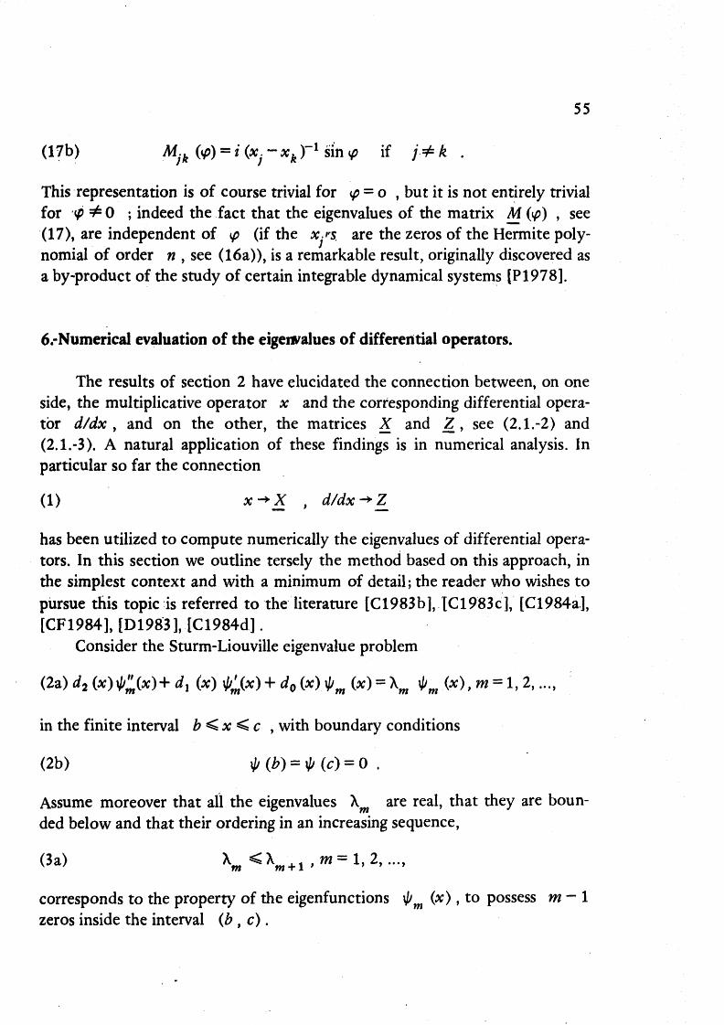
(17b) Mjk (<p) = i (x. - xk ) - 1 sin «p if j^k .

This representation is of course trivial for y = o , but it is not entirely trivial for <p # 0 ; indeed the fact that the eigenvalues of the matrix M (<£) , see (17), are independent of $ (if the x.n. are the zeros of the Hermite poly-nomial of order n , see (16a)), is a remarkable result, originally discovered as a by-product of the study of certain integrable dynamical systems [PI978].

6.-Numerical evaluation of the eigenvalues of differential operators.

The results of section 2 have elucidated the connection between, on one side, the multiplicative operator x and the corresponding differential opera-tòr d/dx , and on the other, the matrices X and Z , see (2.1.-2) and (2.1.-3). A naturai application of these findings is in numerical analysis. In particular so far the connection

(1) x^X , d/dx^Z_

has been utilized to compute numerically the eigenvalues of differential opera­tors. In this section we outline tersely the method based on this approach, in the simplest context and with a minimum of detail; the reader who wishes to pursue this topic is referred to the literature [C1983b], [C1983c], [C1984a], [CF1984], [D1983], [C1984d].

Consider the Sturm-Liouville eigenvalue problem

(2a) d2 (x)^(x)+ dì (x) \(/(*) + d0 (x) tym (x) = Xw * w (x), m = 1, 2,...,

in the finite interval b<x <c , with boundary conditions

(2b) ^ ( ^ ) = ^ ( r ) = o .

Assume moreover that ali the eigenvalues \m are real, that they are boun-ded below and that their ordering in an increasing sequence,

(3a) X <X . - , m = 1, 2,...,

corresponds to the property of the eigenfunctions \pm (x), to possess m - 1 zeros inside the interval (Jb , e).

56

It is then convenient to set

(4) i)m (x) = {x-b)(x-c)vm (x) ,

transforming thereby the eigenvalue problem (2) into the equivalent problem

(5a) ,z/ipm (x) = \m <pm {x) ,

(5b) ip (x) regular at x = b and x = e ,

where stf is the differential operator (singular at x = b and x = e)

(6a) s0 -a2 (x) d2/dx2 + a{ (x) d/dx + a0 (x)

with

(6b) a2 (x) = d2 (x) ,

(6c) ax (x) - dx (x) + 2[(x- b)~x + (x- c)~l ] d2 (x) ,

(6d) a0(x)=d0(x)+[(x-b)~1 -hix-c^ìdi (x)+2[(x~b)(x-c)]~1d2(x).

We then introduce the matrix A , that corresponds to the differential operator stf via (1),

(7) A=a2 {X)7? +ax (X) Z + a0 (X) ,

as well as its eigenvalues and (right and left) eigenvectors,

(8a) AvJm)=am i/m) , m = 1,2,...,^ ,

(8b) u(m)A=a u(m) , m = ì, 2, ..., n. m _

Let us moreover assume that the functions d2 (x) , dx (x) and d0 (x) are entire and that d2 (x) has no zeros (for any complex value of x ) . This implies that the eigenfunctions \j/ (x) are also entire. The generic solution V? (x) of (15a) is not entire; it has a simple pole at x = b and/or at x = e (see (4)). But the eigenfunctions <p x (x) are entire, see (5b); indeed each eigenvalue X is determined by the condition that the singular Sturm-Liou-ville equation (5a) possess an entire solution <p (x) . But the results of sub-

57

section 2.1 (in particular, Corollary 2.1.3) imply that, if <p (x) is a poly-nomial of degree less than n , then one eigenvalue of the matrix A must coincide precisely with X . It is therefore plausible to conjecture that, even if the eigenfunction <p (A:) is not a polynomial, for sufficiently large n , there will be an eigenvalue of A that approximates closely X (since any given entire function \p (x) can be closely approximated, in the interval (b , e), by a polynomial of sufficiently high degree).

A more detailed, if heuristic, analysis of the situation is in order here; for, even if ali the eigenvalues X are real, this is generally not the case for the n eigenvalues of the matrix A . Let us therefore select, out of the n eigenvalues oc , the real eigenvalues (that number, say, v ; of course ^ < n), and let us moreover order them in increasing sequence and cali them X (n)\

(9) X (»)<X A1 (») , w = l , 2, . . . , ! / -1 .

The heuristic conjecture can now be formulated as follows:

(10) lim [X - X (»)] = 0 .

Actually a nonrigorous estimate of the rate of convergence has also been obtained [C1983b], [C1983c],

H - 2 (11) IX - X (n) 1/ IX i ~(Trm/2n)

which applies for an equally spaced choice of the n points x. (that enter in the definitions of the matrices X and Z^ ; see (2.1.- 2,3)). It follows from the formula

(12a) Xm-Xw (n) = (u(m> A(m))/(u(m), w(m))

whére ufm* is the lèft-eigenvector of A corresponding to the eigenvalue X (n) (see (8b))and the w-vectors $(m) and w(m) are defined as follows:

(12b) Ìlnt) = {2a2(xj)^)[x(xr 2))25. + ^ (x.) J»> [x(xp \)}}/{bj n\) ,

(12c) w(m)=^n(xj)/bj .

As for this formula, it obtains easily setting x-xi in (5a), using (2.2.- 5), (2.2- 8) and (2.2.- 10), multiplying from the left by the vector uim) and

58

using (8b). This estimate suggests fast convergence; this is borne out by numerical

tests[D1983], [CF1984]. This approach has been extended to integrodifferential equations [DI983 ],

to multidimensional problems [C1983c], to problems with periodic boundary conditions [C1984a], [C1984d] (sce subsection 2.5), and has been tested with good success in a large set of eigenvalue problems with second order and hi-gher order differential equations in one and more dimensions [CF1984]; al-though much remains to be done, especially to discuss more rigorously the convergence and to introduce improvements. An important improvement, that opens the prospect to get rid of complex eigenvalues, has been indepen-dently suggested by G. Fichera (private communication) and by L. Durand (private communication; including an estimate of the resulting improvement in convergence, corresponding essentially to a doubling of the exponcnt in ther.h.s. of (11)).

As emphasized by G. Fichera (private communication), thistechnique to compute the eigenvalues of differential operators constitutes merely a variant of the classical method of "approximation by points"; we submit that its main merit (if any) rests in its remarkablc simplicity and flexibility (provided by the freedom to choose arbitrarily the n points x. ) . In particular, in contrast to methods based on variational principles such as that of Raleygh-Ritz, that can also be formulated so as to reduce the approximate calculation of the eigenvalues of a differential operator to the computation of the eigen­values of a finite-dimensional matrix, there is no need to perform any integra­tion. On the otherhand variational approximations may yield rigorous bounds, namely approximations known a priori to be by excess or defect, which is not the case for the method described here.

7. - Envoi.

The results reported in this paper are quite elementary, as it behooves to a discussion of such a basic subject as the differential operator d/dx and finite-dimensional matrix representations of it. For the same reason it is likely that some of the results reported in this paper appear vaguely familiar, and perhaps somewhat trivial, to some readers; but we believe it unlikely that most of these results appear familiar hence trivial to most readers. Yet, in view of their basic nature and potential usefulness, this ought to be the case. It is this situation that has provided the main motivation for drafting this review.

59

There are obviously many additional potential applications of these re-sults, both in numerical analysis and elsewhere; for instance the formalism of section 2 provides a convenient tool not only to reobtain the integrable dyna­mical systems discussed in [C1978], but to introduce a much larger class of solvable dynamical systems [C1984c]. The main purpose of this paper is to foster such developments.

REFERENCES

A1980 D. Atkinson: "Inversion of an equation of Calogero". In Problèmes inverses, évolution non linéaire (comptes rendus de la rencontre R. C. P. 264, Montpellier, October 1979; edited by P. C. Sabatier), Editions du CNRS, Paris, 1980, pp. 267-270.

ABCOP1979 S. Ahmed, M. Bruschi, F. Calogero, M. A. Olshanetsky and A. M. Perelomov: "Properties of the zeros of the ólassical polynomials and of the Bessel functions". Nuovo Cimento 49B, 173-199 (1979).

BC1981 M. Bruschi and F. Calogero: "Finite dimensionai matrix representations of the operator of differentiation through the algebra of raising and lowering operators: general properties and explicit examples". Nuovo Cimento 62B, 337-351 (1981).

C1977 F. Calogero: "On the zeros of the classical polynomials". Lett. Nuovo Ci­mento 19, 505-508 (1977).

C1978 F. Calogero: "Motion of poles and zeros of special solutions of nonlinear and linear partial differential equations and related "solvable" many-body problems". Nuovo Cimento 43B, 177-241 (1978).

t

C1979a F. Calogero: "Singular integrai operators with integrai eigenvalues and polynomial eigenfunctions". Nuovo Cimento 51B, 1-14 (1979) & 53B, 463 (1979).

C1979b F. Calogero: "Integrai representations and generating function for the polynomials U&& (*)". Lett. Nuovo Cimento 24, 595-600 (1979).

C1980a F. Calogero: "Isospectral matrices and polynomials". Nuovo Cimento 58B, 169-180(1980).

I

60

C1980b F. Calogero: "Finite transformations of certain isospectral matrices". Lett. Nuovo Cimento 28, 502-504 (1980).

CI98 la F. Calogero: "Matrices, differential operators and polynomiah". J. Math. Phys. 22, 919-9 32 (1981).

C198lb F. Calogero: "Additional identities for certain isospectral matrices". Lett. Nuovo Cimento 30, 342-344 (1981).

C1982a F. Calogero: "Isospectral matrices and classica! polynomiah". Linear Alg. Appi. 44, 55-60(1982).

C1982b F. Calogero: "Disproof of a conjecture". Lett. Nuovo Cimento 35, 181-185

(1982).

C1982c F. Calogero: "Lagrangian interpolation and differentiation". Lett. Nuovo Cimento 35, 273-278(1982).

C198 3a F. Calogero : "Integrable dynamicalsystemsandrelatedmathemàtical results "in Nonlinear Phenomena (Proceedings ot the CIFMO School and Workshop held at Oaxtepec, Mexico, November 29-December 17, 1982; edited by K. B. Wolf), Lecture Notes in Physics 189, Springer, 1983, pp. 47-109.

C1983b F. Calogero: "Computation of Sturm-Liouville eigenvalnes via Lagrangian interpolation". Lett. Nuovo Cimento 37, 9-16 (1983).

CI983e F. Calogero: "Interpolation, differentiation and solution of eigenvalue prò-blems in more than one dimension". Lett. Nuovo Cimento 38, 453-459 (1983).

C1984a F. Calogero: "Interpolation, differentiation and solution of eigenvalue pro-hlems for periodic functions". Lett. Nuovo Cimento 39, 305-311 (1984).

C1984b F. Calogero: "Determinantal represe ntations of the classical polynomiah".

Bolletino U.M.l. (in press).

C1984c F. Calogero: "A class of solvable dynamical systems". Physica D (in press).

C1984d F. Calogero: "Interpolation and differentiation for periodic functions"

Lett. Nuovo Cimento 42, 106-110 (1985).

CF1984 F. Calogero and E. Franco: "Numerica! tests of a novel technìques to com-

pute the eigenvalues of differential operators". (to be published).

CP1978 F. Calogero and A. M. Perelomov. "Asymptotic density of the zeros of

61

Hermite polynomials of diverging arder, and related properties of certain singidar integrai operators". Lett. Nuovo Cimento 23, 650-652 (1978).

CP1979 F. Calogero and A. M. Pcrelomov: "Some diophantine relations involving circidar functions ofrational angles". Linear Alg. Appi. 25, 91-94 (1979).

D1983 L. Durand: "Lagrangian differentiation, integration and eigenvalues pro-blems". Lett. Nuovo Cimento 38, 311-317 (1983).

S1939 G. Szegb: Orthogonal Polynomials. AMS Colloquium Publications 23. Providence, R. I. 1939. (Fourth cdition, second printing, 1978).

1IMF Handbook of Mathematical Functions (M. Abramowitz and I. Stegun, eds.). National Bureau of Standards. Applied Mathematics Series, 55. U.S. Go­vernment Printing Office, 1964.

P1978 A. M. Perelomov: "The simple relation between certain dynamical systems". Commun. Math. Phys 63, 9-11 (1978).

F. CALOGERO, Dipartimento di Fisica, Università di Roma "La Sapienza", 00185 Roma.