Some Applications of WRF/DART

Some Applications of WRF/DART

Chris Snyder, National Center for Atmospheric Research Mesoscale and Microscale Meteorology Division (MMM), and Institue for Mathematics Applied to Geoscience (IMAGe)

WRF/DART

Consists of: –  Interfaces between WRF and DART (e.g. translate state vector, compute

distances, …) –  Observation operators –  Scripts to generate IC ensemble, generate LBC ensemble, advance WRF

Easy to add fields to state vector (e.g. tracers, chem species) –  Plan to add namelist control of fields in state vector

A few external users (5-10) so far

Nested Grids in WRF/DART

Perform analysis across multiple nests simultaneously –  Innovations calculated w.r.t. finest availble grid –  All grid points within localization radius updated

D1

D2

D3

.

. obs

obs

Some Applications

Radar assimilation for convective scales –  Example courtesy Altug Aksoy (NOAA/HRD)

Assimilation of surface observations –  Examples courtesy David Dowell (NCAR) –  Also have single-column version of WRF/DART from Josh Hacker (NCAR)

Tropical cyclones –  Typhoon Sinlaku (2008) example, courtesy Hui Liu (NCAR)

Radar Assimilation for Convective Scales

Assimilate radial velocity and radar reflectivity.

Convective scale: –  O(1 km) horizontal resolution in WRF –  Initialize with single sounding and use open lateral boundaries (thereby

ignoring any mesoscale structure in environment) –  2-min assimilation cycle

Crucial to account for uncertainty in sounding.

Clear biases in reflectivity … owing to errors in microphysics?

Analysis quality comparable to standard dual-Doppler retrievals.

Radar Assimilation for Convective Scales

Aksoy et al. (2008) consider four cases –  Diverse storm types –  Chosen in part based on availability of nearby sounding

Other WRF/DART users are considering additional cases

Storm type Date Location (radar) Supercell 8 May 2003 Oklahoma (KTLX)

Supercell 11 April 2005 Oklahoma (KTLX)

Line, bow echo 15 June 2002 Kansas (KGLD)

Multicell 8 May 2005 Oklahoma (KTLX)

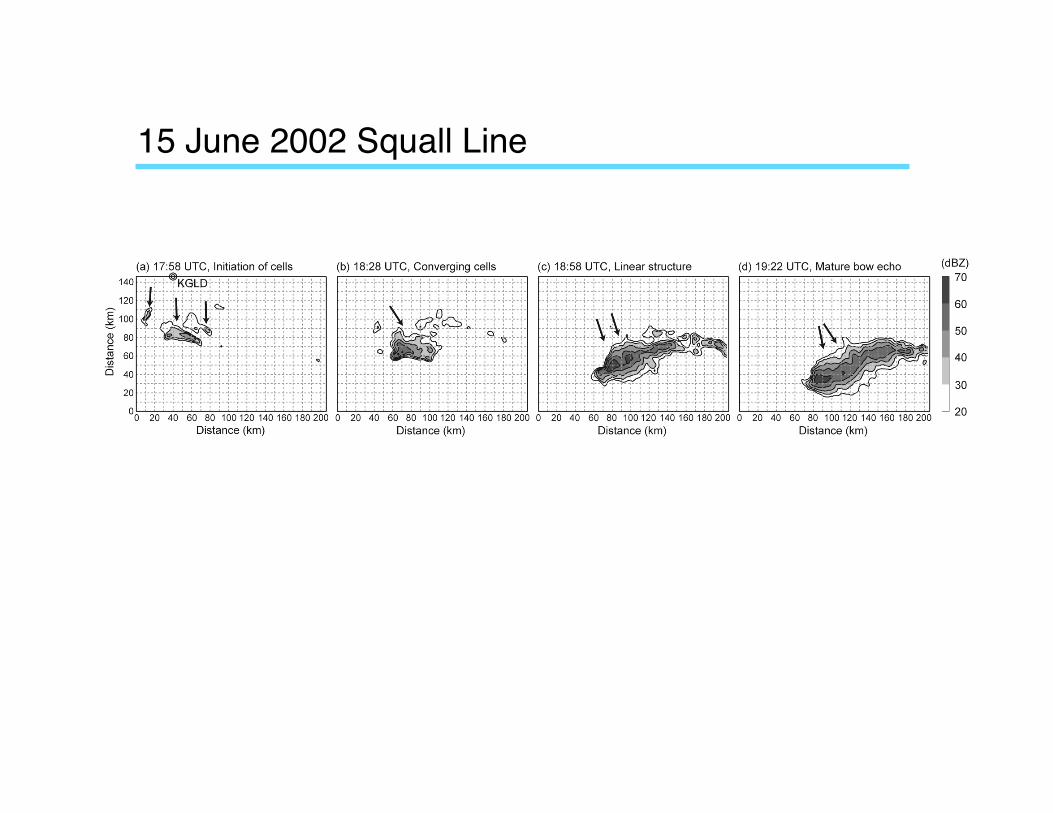
15 June 2002 Squall Line


Innovation statistics


Reflectivity analysis 18:56 UTC (after 60 min assimilation)

Differences from observations

15 June 2002 Squall Line (Forecast)

Reflectivity (dBZ) at 0.5° scan angle

Forecast Observed

6 minutes



Forecast Observed

12 minutes



Forecast Observed

16 minutes



Forecast Observed

22 minutes



Forecast Observed

26 minutes

Assimilation of Surface Observations

30-km resolution, CONUS domain

Hourly assimilation of 2-m T, Td and 10-m u,v –  Assimilate for 9 h, beginning from 00z NAM analysis as ensemble mean

“Multi-physics” ensemble –  Each member uses distinct configuration of WRF –  Choose from 3 PBL, 3 cumulus, 2 shortwave radiation –  Hope to capture, at least partially, uncertainty of forecast model

Perform ensemble forecasts on subdomain with 3-km resolution

Again, see significant problems from deficiencies in model

Supercells in 3-km Ensemble!0000, 0100, and 0200 UTC 29 March 2007! SPC Storm Reports!

28-29 March 2007: With and Without Surface-Data Assimilation!

no assim + 12-14 hr fcst! 9 hr sfc DA + 3-5 hr fcst!







Results of Surface-Data Assimilation on 30-km grid: !Water Vapor at 30 m AGL, 2100 UTC 28 March 2007 !

Ensemble-Mean Analysis!with sfc data assimilation!

Analysis Difference:!(ens mean with sfc data assim)!- (ens mean without sfc data assim)!

ensemble-mean T and Td profiles at 1800 UTC 12 June 2002

with sfc DA

without sfc DA 1000 mb

850 mb

700 mb

WRF

ens

embl

e,

no a

ssim

ilatio

n O

bser

vatio

ns

FWD

0000

UTC

WRF

ens

embl

e,

no a

ssim

ilatio

n O

bser

vatio

ns

OUN

000

0 UT

C

6 hr sfc DA + 3 hr fcst

2100 UTC 12 June 2002

too early

•  EnKF uses ensemble-estimated vertical covariances to determine how surface observation influences analysis of PBL

•  Analysis is biased if forecast profiles all have the wrong shape in ~ same way

surface dewpoint ob

forecast

actual profile

analysis

Surface DA in Presence of Model Bias

Outstanding Issues

Model imperfections, including errors in sub-grid processes —  Essential to account for these in mesoscale assimilation —  Multi-physics, adaptive inflation, additive noise …

Wish to estimate and predict across range of scales —  Require better techniques for covariance localization, or alternate

approach

Nonlinearity and non-Gaussianity —  So far, dynamical nonlinearities not alarming —  Bigger problems with positive-definite quantities?

References

Bengtsson T., C. Snyder, and D. Nychka, 2003: Toward a nonlinear ensemble filter for high-dimensional systems. J. Geophys. Res., 62(D24), 8775-8785.

Dowell, D., F. Zhang, L. Wicker, C. Snyder and N. A. Crook, 2004: Wind and thermodynamic retrievals in the 17 May 1981 Arcadia, Oklahoma supercell: Ensemble Kalman filter experiments. Mon. Wea. Rev., 132, 1982-2005.

Snyder, C. and F. Zhang, 2003: Assimilation of simulated Doppler radar observations with an ensemble Kalman filter. Mon. Wea. Rev., 131, 1663-1677.

Torn, R. D., G. J. Hakim, and C. Snyder, 2006: Boundary conditions for limited-area ensemble Kalman filters. Mon. Wea. Rev., 134, 2490-2502.

Hacker, J. P., and C. Snyder, 2005: Ensemble Kalman filter assimilation of fixed screen-height observations in a parameterized PBL. Mon. Wea. Rev., 133, 3260-3275.

Caya, A., J. Sun and C. Snyder, 2005: A comparison between the 4D-Var and the ensemble Kalman filter techniques for radar data assimilation. Mon. Wea. Rev., 133, 3081-3094.

Chen, Y., and C. Snyder, 2007: Assimilating vortex position with an ensemble Kalman filter. Mon. Wea. Rev., 135, 1828-1845.

Anderson, J. L., 2007: An adaptive covariance inflation error correction algorithm for ensemble filters. Tellus A, 59, 210-224.

Snyder, C. T. Bengtsson, P. Bickel and J. L. Anderson, 2008: Obstacles to high-dimensional particle filtering. Mon. Wea. Rev., accepted.

http://www.mmm.ucar.edu/people/snyder/papers/

EnKF Applied to Convective Storms

Model and EnKF details –  Open lateral BCs, no terrain or PBL, Lin et al. microphysics –  Horizontal resolution 2 km, vertical resolution 500 m –  ~ 2 min cycling … assimilate scan at each elevation angle separately –  50 members

Observations –  Radial velocity and reflecitivity on each elevation angle –  Removal of clutter, other simple QC from Dowell/NSSL package –  Obs on each elevation angle pre-processed to ~ model grid in horizontal –  Distinguish reflectivity > 5 dBZ (precip) from < 5 dBZ (clear air)

Automated velocity unfolding within EnKF

15 June 2002 Squall Line (Forecast) Reflectivity (dBZ) at 2.4° scan angle (24-min forecast)

15 June 2002 Squall Line (Sounding Perturbations)

U Component V Component


Innovation statistics – impact of perturbing the sounding


Reflectivity (dBZ) at 4.3° scan angle (60-min analysis, 18:56 UTC)

Without Sounding Pert. With Sounding Pert.

Ensemble Initialization

ICs include random temperature perturbations –  Restricted to neighborhood of first echoes to be assimlated

Uncertainty in sounding/environment –  (u,v) sounding for each member includes noise in three gravest vertical

modes, with variance 2 m/s in each mode –  At present, not perturbing θ or moisture

Comparison of EnKF and 4DVar

•  Simulated observations of radial velocity and reflectivity for supercell storm (perfect model), available every 5 min

•  4DVar: full fields (not incremental), mesoscale background, simple covariance model, 10-min window

•  EnKF: 100 members, initialized with noise in T where first scan shows reflectivity

Caya, A., J. Sun and C. Snyder, 2005: A comparison between the 4D-Var and the ensemble Kalman filter techniques for radar data assimilation. Mon. Wea. Rev., 133, 3081--3094.

Comparison of EnKF and 4DVar

Kalman filter/smoother and 4DVar are mathematically equivalent for linear, Gaussian systems –  Result also assumes both use same P, R, etc.

Overall, EnKF and 4DVar perform comparably in this case

After multiple cycles (30-40 min), EnKF beats 4DVar –  EnKF propagates information from previous obs through cycling of Pf –  In principle, updating of P could be included in 4DVar too

Given only obs over limited period (10-20 min), 4DVar beats EnKF –  Estimation errors large with limited obs, so nonlinear effect more important

and 4DVar has advantage?

Mesoscale and Storm-Scale Ensemble Forecasts!

surface ob site!

regional (storm-scale)!"domain (Δx=3 km)!

mesoscale domain!"(Δx=30 km)!

30-km ensemble provides initial and boundary conditions for 3-km ensemble!

Appeal of Ensemble Filters for Mesoscale DA

General covariance model •  Independent of assumptions about nature of flow (e.g. approximate

geostrophic balance), applicable across variety of dynamical regimes

Basis for probabilistic forecasts •  For convective storms, 1 hour is a long-range forecast

Ease of implementation and maintenance •  Doesnʼt require adjoints for sub-grid schemes, which are crucial in these

flows but often discontinuous or highly nonlinear •  … or adjoints of complex observation operators (e.g. radar) •  See http://www.met.tamu.edu/people/faculty/fzhang/EnDA2006/

Straightforward application to domains with multiple nests

Nonlinearity and non-Gaussianity

EnKF uses only second moments; can find non-Gaussian examples where EnKF is not effective.

At same time, EnKF is not strictly a “Gaussian” method –  Can find examples where resampling from same mean and covariance as

EnKF posterior does much worse than EnKF (Bengtsson et al. 2003) –  EnKF thus preserves some useful information about higher moments

Particle filters are a fully general, non-parametric approach. –  But they fail in high dimensions unless sample size is v. large (Snyder et al.

2008)

Is there a way to perform spatially local updates in nonlinear ensemble filters, as in the EnKF?

Documents

Some Applications of WRF/DART