Extracting Human Behavior Patterns fromAppliance-level Power Consumption Data

Alaa Alhamoud1, Pei Xu1, Frank Englert1, Andreas Reinhardt2, PhilippScholl3?, Doreen Boehnstedt1, and Ralf Steinmetz1

1 Multimedia Communications LabTechnische Universitat Darmstadt, Darmstadt, Germany,

firstname.lastname @kom.tu-darmstadt.de2 Department of Informatics

Technische Universtitat Clausthal, Clausthal-Zellerfeld, Germanyreinhardt@ieee.org

3 SAP AG, Walldorf, Germanypscholl@gmail.com

Abstract

In order to provide useful energy saving recommendations, energy managementsystems need a deep insight in the context of energy consumption. Getting thoseinsights is rather difficult. Either exhaustive user questionnaires or the installa-tion of hundreds of sensors are required in order to acquire this data. Measuringthe energy consumption of a household is however required in order to find andrealize saving potentials. Thus, we show how to gain insights in the context ofenergy consumption directly from the energy consumption profile. Our proposedmethods are capable of determining the user’s current activity with an accuracyup to 98% as well as the user’s current place in a house with an accuracy up to97%. Furthermore, our solution is capable of detecting anomalies in the energyconsumption behavior. All this is mainly achieved with the energy consumptionprofile.

1 Introduction

The realization of energy efficiency in buildings has become an important re-search topic in industrial as well as research community. The main motivationfor this increasing importance is the conservation of energy in a world whereenergy prices are always fluctuating and very sensitive to political as well asnatural crises. This is also driven by the wide spread of wireless sensor networkswhich made it possible to collect fine-grained data about the building contextas well as the context of its inhabitants. In this paper, we develop three novelexperiments which exploit the huge information provided by the smart home

? Co-author is employed by SAP AG; however, the opinions and results expressed inthis paper are his own and do not denote the point of view of SAP AG.

to achieve the main goal of our research efforts which is to conserve energy insmart homes while maintaining user comfort. The main focus of our work inthis paper is the analysis of our smart home dataset which we call from nowon SMARTENERGY.KOM dataset4. SMARTENERGY.KOM dataset is a largedataset which contains about 42 million data points of sensor readings and userfeedback which we have collected from two smart home environments for theprimary purpose of detecting human activities based on wireless sensor net-works [2], thus to save unnecessary consumed energy. In the first deployment, awireless sensor network was deployed for about 82 days. More than 22 millionactivity related sensor events were generated by corresponding sensors. The du-ration of deployment 2 was about two months, during which about 20 millionsensor readings were recorded. We have used two types of wireless sensor nodesin both deployments. On one hand we deployed Plugwise5 sensors for sensing theappliance-level power consumption of the household. Each device in the housewas connected to a Plugwise sensor which measures the load of the device. Onthe other hand we deployed Pikkerton6 sensors for sensing the temperature,brightness as well as the motion in the environment. In both deployments, ninedaily user activities were monitored:Deployment 1 : Sleeping, Watching TV, Not at Home, Reading, Eating, Cook-ing, Working at PC, Making Coffee and Cleaning Dishes.Deployment 2 : Sleeping, Watching TV, Not at Home, Reading, Eating, Mak-ing Tea, Listening Radio, Slicing Bread and Ironing.These activities have been chosen based on the available electrical applianceswhich can be monitored at home. Some of these activities like “Watching TV”can be directly related to the power consumption. Other activities such as “Sleep-ing” and “Not at Home” can be indirectly inferred from the power consumption.This list of activities does not necessarily contain all the activities performed bythe user at home. Therefore, we have provided the user with the option “Ignore”which implies as a feedback that the user’s current activity does not belongto the list of activities provided by us. This option helps preserving the pri-vacy of the user as well by giving her/him the choice whether to report her/hiscurrent activity or not. All sensor readings which are related to the option “Ig-nore” have been excluded from the dataset before conducting our experiments.Based on these two deployments, we have built an activity detection frameworkwhich uses the feedback provided by the user to learn his current activity andrelate it to the collected sensor readings. The remainder of this paper is struc-tured as follows. Section 2 surveys related research projects whose main focusis the analysis of datasets collected by wireless sensor networks in the contextof smart home. In Section 3, we present our novel concept for user localizationin indoor environments based on real-time appliance-level power consumption.In Section 4, we analyze the temporal relations between the user activities and

4 The dataset is available for download under: http://www.kom.tu-darmstadt.de/

research-results/software-downloads/software/smartenergykom5 http://www.plugwise.com/6 http://www.pikkerton.com/

examine whether the discovered relations could increase the accuracy of ouractivity detection framework. In Section 5, we analyze the user’s daily powerconsumption behavior. We conclude the paper in Section 6.

2 Related Work

In recent years, analyzing datasets collected from wireless sensor networks insmart homes has become of great interest to computer science researchers. Thisis mainly driven by the great potential offered by these datasets for developingIT services which can improve the life quality as well as the energy efficiency ofthe smart homes. Data mining techniques have been utilized in order to extractall the possible useful hidden patterns contained in such datasets. In the workof Chen et al. [4], they analyzed a dataset which contains more than 100,000sensor events collected from two apartments. The primary purpose of their workwas to recognize human activities performed in these two apartments and under-stand the related energy usage. They applied clustering techniques for identifyingthe normal power consumption patterns, thus to detect abnormal energy usage.Using classification techniques, they trained a model for predicting the energyusage of an inhabitant based on her/his currently performed activities. Anotherexample is given by Hoque et al. [8], where 26 days of activity related sensorevents collected from a single resident home is analyzed. Based on the hypoth-esis that each activity will trigger a set of specific sensors, they applied patternmining to find all simultaneously fired sensors. In the next step, different to [4],clustering is used for discovering events based on previously extracted patterns.Besides, they utilized clustering for labeling the instances. Finally, they build aclassification model for recognizing the activities. Fogarty et al. [6] analyzed 3.4million sensor readings from a home shared by two adults. Their goal was to de-tect water usage related activities by configuring microphone based sensors thatlisten for the water flow into and out of a home. They applied the classificationalgorithm support vector machine to train a model for recognizing different typesof water usage. Fluctuations of sound waves returned by the sensors are consid-ered as features for training the classification model. Activated sensors togetherwith their temporal characteristics are then combined to form patterns for iden-tifying the activities. Different from the aforementioned research projects, ouranalysis is conducted on a much larger dataset. Moreover, the three experimentsconducted in our work have not been covered by any of these research worksalthough similar data mining techniques are utilized.

3 Sensing Power Consumption for User Localization

User localization has always been one of the central challenges in the designof smart home environments. A wide variety of sensors such as Passive Infraredsensors can be used in order to achieve this goal. Currently, the usage of electric-ity consumption data for occupancy detection started to gain attention among

the research community as we see in [11] where the authors used the data col-lected from smart meters for the purpose of occupancy detection. This leads usto the idea of utilizing new kind of sensors for user localization in smart home,namely the appliance-level power sensors which sense the power consumption ofindividual household appliances. Therefore, in this paper we examine the usageof these sensors for the purpose of user localization in smart home where we aimat localizing users with a better resolution than shown in [11]. Usually, users per-form specific activities in specific places, such as cooking in the kitchen, sleepingin the sleeping room and so on. Therefore, each activity is associated with cer-tain appliances which consume energy during this activity. In other words, byknowing the devices which are consuming energy, we can infer the location ofthe user in the smart home. In order to verify this theory, we use supervisedlearning techniques where the input of the classification model will be the user’sreal-time appliance-level power consumption and the output is the location ofthe user. In the following sections, we explain the construction of the training setfor the supervised learning model and we evaluate the accuracy of this model.

3.1 Construction of the Training Set

The first step in supervised learning is to construct a training set for buildingthe classification model. As mentioned before, each user’s location in the smarthome is accompanied with a set of sensor readings representing the real-timeappliance-level power consumption. These sensor readings represent the inputfor the supervised learning model along with the labels which represent the user’slocation. Sensor readings were recorded every ten seconds during the deployment.However, activities normally last for several minutes or even hours e.g. sleeping.In other words, if we directly construct a training set from these sensor readings,the size of the training set will be extremely large leading to an inefficient modelconstruction. Therefore, we need to reduce the size of the training set withoutaffecting the accuracy of the trained classification model. To this end, we dividethe whole time series of sensor readings into timeslots of two minutes. We chosethe period of two minutes as it helps achieving a good accuracy while minimizingthe overlapping between activities in one timeslot. Then, for each sensor, weextracted its maximum value in each timeslot as one feature for constructing thefeature vector. This means, every two minutes will represent a training instancein which the features are the maximum values of sensor readings during thistimeslot. In order to provide the labels of the training instances, we relied onthe user feedback which informs us about the user current activity. By knowingthe current user activity, we can infer the current location of the user, becauseeach activity is performed in one and only one location. The labeling processmainly relies on the time interval between one activity and the next activity,namely the duration of each activity. Therefore, by examining in which timeinterval the timestamp of an instance is falling into, we can assign the locationof the corresponding activity in that time interval to the instance. The finalgenerated form of the instances is shown in Eq. 1, where Sn max(sloti) meansthe maximum sensor value of sensor n in ith timeslot, and m is the total number

of timeslots. Therefore, the training set is composed by a set of such instances< I1, I2, ..., Im >.

Ii =< S1 max (sloti) , S2 max (sloti) , ..., Sn max (sloti) ,

Class(sloti) > i ∈ [1,m](1)

3.2 Building and Evaluation of the Classification Model

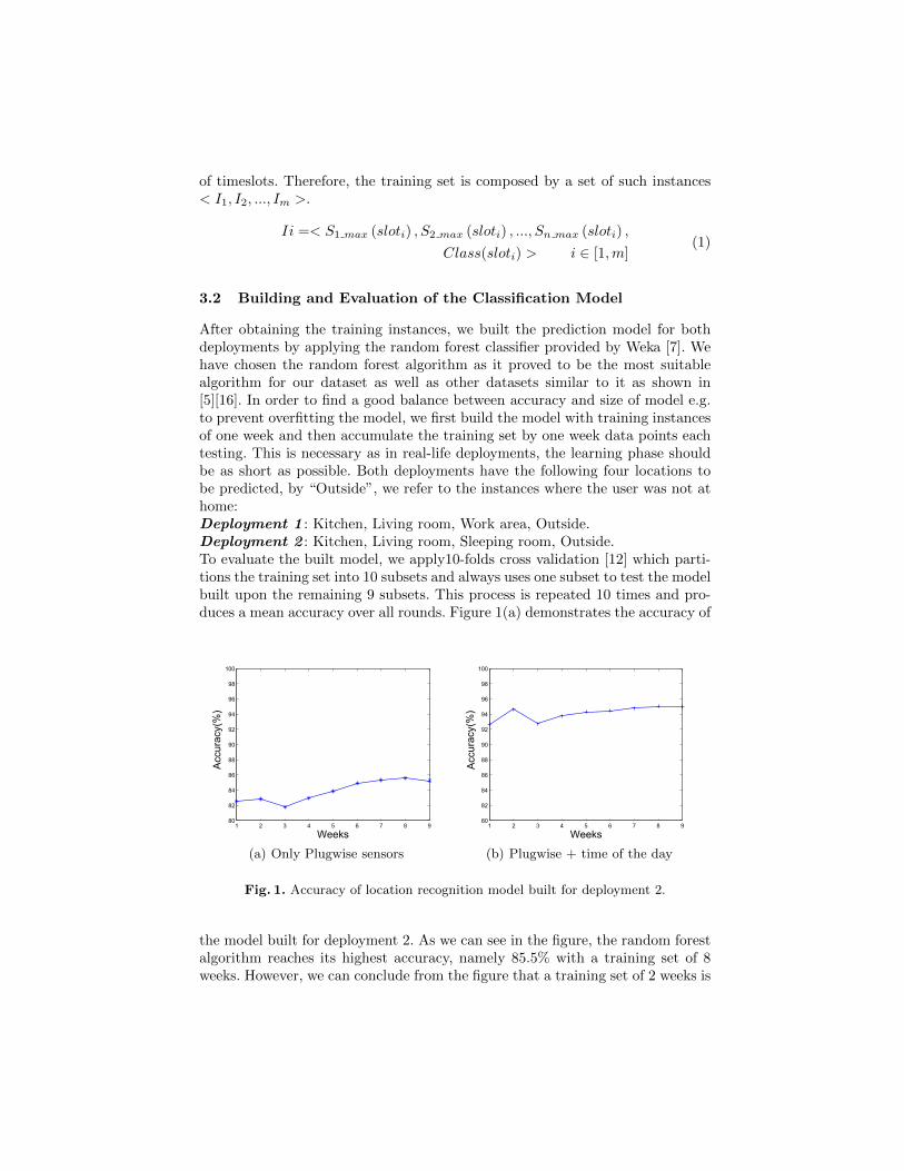
After obtaining the training instances, we built the prediction model for bothdeployments by applying the random forest classifier provided by Weka [7]. Wehave chosen the random forest algorithm as it proved to be the most suitablealgorithm for our dataset as well as other datasets similar to it as shown in[5][16]. In order to find a good balance between accuracy and size of model e.g.to prevent overfitting the model, we first build the model with training instancesof one week and then accumulate the training set by one week data points eachtesting. This is necessary as in real-life deployments, the learning phase shouldbe as short as possible. Both deployments have the following four locations tobe predicted, by “Outside”, we refer to the instances where the user was not athome:Deployment 1 : Kitchen, Living room, Work area, Outside.Deployment 2 : Kitchen, Living room, Sleeping room, Outside.To evaluate the built model, we apply10-folds cross validation [12] which parti-tions the training set into 10 subsets and always uses one subset to test the modelbuilt upon the remaining 9 subsets. This process is repeated 10 times and pro-duces a mean accuracy over all rounds. Figure 1(a) demonstrates the accuracy of

1 2 3 4 5 6 7 8 980

82

84

86

88

90

92

94

96

98

100

Weeks

Accuracy(%)

Weeks

Accuracy(%)

(a) Only Plugwise sensors

1 2 3 4 5 6 7 8 980

82

84

86

88

90

92

94

96

98

100

Weeks

Accuracy(%)

Weeks

Accuracy(%)

(b) Plugwise + time of the day

Fig. 1. Accuracy of location recognition model built for deployment 2.

the model built for deployment 2. As we can see in the figure, the random forestalgorithm reaches its highest accuracy, namely 85.5% with a training set of 8weeks. However, we can conclude from the figure that a training set of 2 weeks is

Table 1. Accuracy by classes for deployment 2 by using two weeks dataset

Classes Precision Recall F-Measure

(K)itchen 87.40% 49.30% 64.10%

(S)leeping room 76.70% 99.80% 86.80%

(L)iving room 97.70% 94.10% 95.90%

(O)utside 0.00% 0.00% 0.00%

Table 2. Confusion matrix for deployment 2 by using two weeks dataset

(K) (S) (L) (O)

(K) 49.33% 44.91% 5.76% 0.00%

(S) 0.10% 99.83% 0.07% 0.00%

(L) 2.11% 3.82% 94.08% 0.00%

(O) 0.34% 99.49% 0.17% 0.00%

already sufficient for acquiring a high accuracy. This conclusion is based on thefact that the accuracy only rises about 2.5% when the number of weeks includedin the training set increases from 2 weeks to 8 weeks. This conclusion allows usto shorten the duration of the data collection process in the deployments to comewhich lessens the burden on the user in providing feedback and therefore leadsto a more acceptance of the system. In order to obtain a better understandingof the classification accuracy, we list the precision, recall, and F-measure valuesfor each location in Table 1. Moreover, we show the associated confusion ma-trix in Table 2. The result represents the model built for deployment 2 with atraining set of 2 weeks. Although the overall accuracy reached by this model is83% (cf. Figure 1(a)), the recall values of the classes “Kitchen” and “Outside”are very low with 49.3% and 0% respectively as shown in Table 1. In order tounderstand the reasons for this phenomenon, we have to look on the confusionmatrix in Table 2. From the confusion matrix, we can see that 44.91% of theinstances of the class “Kitchen” have been falsely classified as “Sleeping room”instances. Besides, almost all the instances of the class “Outside” have also beenfalsely classified as “Sleeping room” instances. This can be explained based onthe following facts. First of all, the confusion between the classes “Outside” and“Sleeping room” can be returned to the fact that when the user is outside orsleeping, all Plugwise sensors were almost keeping in silence as no appliances arerequired to perform these activities. Although, there are some values of Plug-wise sensors (e.g. lamp sensor) related to the “Sleeping room” class stored in thedataset, the lamp was in most cases not turned on while sleeping. Furthermore,the instance of the class “Outside” were classified as “Sleeping room” and not theother way around because “Sleeping room” is a dominant class. This is due to thefact that the duration of sleeping is much longer than that of being outside in thisdeployment which leads to more training instances for the class “Sleeping room”than for the class “Outside”. The activity of “Eating” was the major reason offalsely classifying instances of “Kitchen” into “Sleeping room”. This activity issupposed to be identified through the Plugwise sensor connected to the radio in

Table 3. Accuracy by classes for deployment 2 by using two weeks dataset (with time)

Classes Precision Recall F-Measure

(K)itchen 81.80% 73.30% 73.30%

(S)leeping room 98.20% 99% 98.60%

(L)iving room 96.10% 96.80% 96.50%

(O)utside 83.50% 86.30% 84.90%

Table 4. Confusion matrix for deployment 2 by using two weeks dataset (with time)

(K) (S) (L) (O)

(K) 73.32% 9.59% 4.99% 12.09%

(S) 0.99% 98.97% 0.03% 0.0%

(L) 0.65% 0.0% 96.84% 2.50%

(O) 7.77% 0.33% 5.57% 86.31%

the kitchen. However, the radio was not always turned on or only turned on fora part of time during the activity of “Eating”. To solve this problem, we needa strong discriminator which can help distinguishing the classes “Outside” and“Sleeping room”. We thought about a feature which can be used in the learningprocess in order to achieve this task. One feature which can fully perform thisrole is the time of the day. By using the time of the day as a feature for buildingthe machine learning model, we add a strong discriminator especially betweenthe classes “Outside” and “Sleeping room”. We use the “hh:mm:ss” time formatas Weka can deal with this time format automatically. After using the time asa feature in addition to the previous features, the overall accuracy of the modelhas increased as shown in Figure 1(b). To better understand the effect of addingthe time to the feature set, we present the precision, recall, and F-measure valuesfor each location in Table 3. Furthermore, we present the associated confusionmatrix in Table 4. The results in these two tables have been achieved for de-ployment 2 with a training set of 2 weeks. As we can see from Table 3 andTable 4, the time has functioned as a strong discriminator between the class“Sleeping room” and the classes “Outside” and “Kitchen” respectively. The useof the time as a feature makes it easy to solve the confusion between the class“Sleeping room” and the class “Outside” as the user in deployment 2 alwaysgoes outside during the day and not during the night. The location “Kitchen”can also benefit from the usage of time as a feature, because the user performsmost of his activities in the kitchen during the day.

4 Mining Human Behavioral Patterns

As humans tend to follow a regular routine in their daily life, their everydayactivities tend to happen in a certain order which mostly repeats itself every-day. Discovering temporal relations between these daily activities may assist inenhancing the accuracy of our activity detection framework. Hence, in this sec-tion, we first try to detect any behavioral patterns which might exist in the data

collected in both deployments and then we examine whether these detected pat-terns can help increasing the accuracy of the activity detection framework wehave previously developed.

4.1 Extraction of Temporal Activity Patterns

As mentioned in [3], temporal relations between two activities (A, B) can be rep-resented as A happens after B, before B, overlaps with B and so on. According tothe user feedback in both deployments, activities were performed consecutivelyone after another which was a precondition for our dataset. Hence, we only ex-amine the “before” and “after” relations between two activities. In the followingsection, we introduce four terms related to the analysis before explaining theoperations of the pattern mining process.Episode: According to [15], an episode is characterized by a pair of begin andend timestamps, during which one or more activities can happen. As the user’sdaily activities are the major interest of our analysis, we specify the duration ofan episode as a single day. Hence, an episode is composed of all activities per-formed during the day, namely all the activities between timestamps [00:00:00,23:59:59]. This concept is expressed in Eq. 2, where A represents one activity, T isthe associated timestamp, n is the number of activities of the day, while d refersto the number of days in that deployment. After that, we construct an episodedataset by collecting all episodes during the whole deployment. By examiningthe dataset, we obtained 64 valid days for deployment 1 and 61 valid days fordeployment 2. Days of deployment 1 are much less than the actual duration ofthe deployment (about 82 days). This is due to the fact that the feedback wasnot provided by the user in the last 18 days.

Episodei =< A1(T1), A2(T2), ..., An(Tn) > i ∈ [1, d] (2)

Sequence: A sequence is formed by at least two successively performed activi-ties. For instance, <Eating, WatchingTV> means the activity “Watching TV”happens directly after “Eating”.

4.2 Apriori Algorithm

For the extraction of the temporal relations between activities, we apply theApriori algorithm [1] which aims to discover frequent activity sequences basedon what is called their support and confidence:Support: In our case, support measures the frequency of an activity sequenceappearing in the episodes dataset. It is computed as the number of episodesthat contain this sequence, divided by the total number of episodes (Eq. 3). Afrequent sequence can be defined as a sequence whose support is larger than apredefined threshold (minSupp).

Support(< A,B >) =#episodesContaining < A,B >

#episodes(3)

Table 5. Examples of temporal activity patterns

A Cooking Eating Making Coffee

B Eating WorkingAtPC Eating

Supp. (%) 25.0 51.6 28.2

Conf. (%) 84.2 67.4 53.1

Confidence: It represents the dependency between two activities i.e. the proba-bility that one activity occurs given that a certain previous activity has occurred.Hence, confidence for the sequence <A, B> is computed as the support of <A,B> divided by the support of A. The main principle of the Apriori algorithm isto scan the whole episodes dataset in order to find all frequent items (activities)and exclude those which are rarely performed. However, a rarely performed ac-tivity does not necessarily imply the nonexistence of a regular temporal activitypattern which involves this activity. An example from our dataset is the “Read-ing” activity. This activity has a support of 4.7% in deployment 1. However, ifthe user always sleeps after reading, then the sequence <Reading, Sleeping> canalso be considered as a meaningful pattern due to its high confidence. As shownabove, a threshold has to be specified which determines the minimum value thesupport of a sequence should have in order to be considered by the Apriori algo-rithm as a regular sequence. This threshold is called the minSupp. On one hand,a high minSupp value might cause the exclusion of meaningful patterns becauseit involves activities with low support value. On the other hand, a small minSuppvalue might cause the generation of a numerous number of meaningless patternsby the Apriori algorithm. In order to overcome this problem, we utilize the mul-tiple minimum supports mechanism [14]. This mechanism assigns a miniSuppito each item (Ai) by multiplying a user defined global miniSupp by the item’sown support as shown in Eq. 4. By doing this, useful patterns regarding to therarely performed activities will not be neglected during the process. Meanwhile,patterns regarding to one activity with support lower than the assigned minSuppwill be filtered out. Therefore, we define the global minsupp as 18%.

minSuppi = global minsupp× support(Ai) (4)

By applying Apriori algorithm, we obtained a list of temporal activity patternsfor each deployment. Table 5 lists some of the extracted patterns from the firstdeployment where A denotes the previous activity and B denotes the currentactivity. As we can see from the table, the user usually starts with the eatingactivity directly after cooking with a confidence of 84.2%. After eating he oftenworks at PC with a confidence of 67.4%. The activity after making coffee isalso eating with a confidence of 53.1%. These examples show the existence of acertain routine in our daily life. In the following section, we use the extractedpatterns in the activity detection process in order to see if it can help improvingthe accuracy of this process.

Table 6. Activity detection accuracy with and without patterns (random forest)

Deployment 1 Deployment 2

Accuracy F-Measure Accuracy F-Measure

without 92.8% 92.7% 97.3% 97.3%

with 96.1% 96.1% 98.3% 98.3%

KOM – Multimedia Communications Lab 16Pei Xu

0

20

40

60

80

100

Accu

rac

y (

%)

MaxValue MaxValue + patterns

Fig. 2. Activity detection accuracy by classes, results of with and without patterns arecompared.

4.3 Utilizing Patterns in Activity Detection

In this step, we integrate the patterns extracted by Apriori algorithm as extrafeatures in building the activity prediction model. The features we used forthe activity detection process were the maximum sensor values (Plugwise andPikkerton) in timeslots of two minutes. As extra features, we added the previousactivity combined with the most likely current activity as it appears in thesequences extracted by Apriori algorithm. Hence, the new feature vector is acombination of all these features as shown in Eq. 5, where An−1 and An representthe previous and the most probable current activity respectively. For labelingthe instances, we use the user feedback denoted as Class(sloti).

Instancei =< S1 max(sloti), S2 max(sloti), ..., Sn max(sloti),

An−1, An, Class(sloti) > i ∈ [1,m](5)

Table 6 shows the accuracy of the activity detection process for both deploy-ments before and after adding the patterns extracted by Apriori algorithm. Theused classification algorithm is random forest. The overall accuracy explicitlyincreases after adding the patterns. Furthermore and in order to obtain a morecomprehensive representation of the classification accuracy for each individualactivity, Figure 2 shows the results coming from deployment 2 using random for-est. As we can see in Figure 2, the detection accuracy of each activity has alsoexplicitly increased after adding the patterns. The reason for this improvement is

that, besides the intrinsic features of the activities, namely the sensor readings,the machine learner will also learn the temporal relations between the activitiesfrom the patterns, thus recognize activities that occur in certain patterns moreaccurately.

5 Analysis of the Daily Power Consumption Traces

In this section we focus on the analysis of daily power consumption traces in ourtwo deployments. The main goal is to understand the daily power consumptionof individuals in smart homes and to find out based on time series analysis if thepeople follow a regular power consumption pattern which repeats itself over thedays. The result of this analysis can be of great importance in many applicationscenarios: it can help developing applications which allow individuals living insmart homes to inspect their energy usage over the time leading to a moreenergy-aware power consumption behavior. Besides, it can be of great benefitto utility companies which by knowing the power consumption behavior of theircustomers can recommend a more suitable tariff and direct the smart grid towork more efficiently, thus to save energy.

5.1 Obtaining Hourly Power Consumption of Each Day

For the analysis to be conducted, we first need to compute the hourly powerconsumption of each day. We calculate the power consumption for each hourby summing up the power consumption within all timeslots of two minutes inthat hour. However, since Plugwise values are stored in unit “Watt”, we needto convert them into “Wh” (Watt hour) for acquiring the power consumption.To do this, we first compute the associated power consumption of each Plugwisesensor in each timeslot. This is achieved by averaging the readings of each sensorin that timeslot and dividing the average value by 30. We divided the averageby 30 as we only need the power consumption in timeslots of two minutes.Then, for obtaining the total power consumption in each timeslot we sum allthe converted values of the Plugwise sensors in that timeslot. The computationis indicated in Eq. 6, where j denotes the sensorId, i denotes the ith timeslot,Sj(Sloti) denotes the average value of sensor j during timeslot i, and n denotesthe number of sensors. To compute the total power consumption in an hour, wesum up the power consumption in all timeslots within that hour as indicated inEq. 7 where m denotes the number of timeslots, and h denotes the hour of theday.

Psloti =

n∑j=1

Sj(Sloti)

30(6)

Ph =

m∑i=1

Psloti h ∈ [1, 24] (7)

1 2 3 4 5 6 7 8 9 10 11 12 13 14 15 16 17 18 19 20 21 22 23 240

50

100

150

200

250

300

350

Hour9of9a9day(h)P

ower

9con

sum

ptio

n(W

h)

06.04.2013

Hour9of9a9day(h)P

ower

9con

sum

ptio

n(W

h)

Fig. 3. Power consumption with regard to the hours of the day on 2013-04-06 fromdeployment 1.

1 2 3 4 5 6 7 8 9 10 11 12 13 14 15 16 17 18 19 20 21 22 23 24−1.5

−1

−0.5

0

0.5

1

1.5

2

2.5

Hour7of7a7day(h)

Sta

ndar

dize

d7po

wer

7con

sum

ptio

n7va

lue

06.04.2013

21.05.2013

Hour7of7a7day(h)Nor

mal

ized

7po

wer

7con

sum

ptio

n7va

lue

Fig. 4. Hourly power consumption distributions on 2013-04-06 and 2013-05-21 fromdeployment 1, consumption values are normalized.

To make the results more comprehensive, we plot the obtained hourly powerconsumption for each day. Figure 3 shows an example in which we see thatthe user consumes more energy from 01:00 pm to midnight than from 3:00 amto noon. When comparing this distribution to another one obtained from thesame deployment as shown in Figure 4, we can easily observe the similarity be-tween these two distributions. In both days, the user followed a similar powerconsumption pattern only shifted in time. The values in the figure are all nor-malized so that they have a mean of zero and a standard deviation of one for thepurpose of comparison. Based on our observation from Figure 4, we conduct asimilarity comparison process on all the distributions which belong to the samedeployment. By verifying that all the distributions from the same deploymentfollow some level of similarity, we can prove the user to have a regular powerconsumption behavior which is the goal of this experiment as stated before. Inthe following section, we introduce the process of similarity comparison, the usedalgorithm, as well as the obtained results.

Similarity =1

1 + warping score(8)

5.2 Similarity Comparison

Similarity comparison between two time series can be conducted using severalalgorithms. One of the these popular algorithms is the approach of symbolicrepresentation [13] in which we convert each time series into a sequence of sym-bols and calculate the distance of these resulting sequences of symbols. Themain disadvantage of this approach is that it does not take time shifting intoconsideration. Thus, it will not recognize two series like the ones shown in Fig-ure 4 similar to each other only because they are shifted in time. In order toaddress this problem, we apply the Dynamic Time Warping (DTW) algorithm[10] which aims to find the best alignment between two time series. The result isrepresented by a warping path that indicates how each point of one distributionis aligned to the point of another distribution. Besides, it also produces a warp-ing score to indicate the distance between two distributions after the alignment.In order to verify the similarity between each pair of distributions, we convertedthe warping score into a similarity measure based on Eq. 8 as clarified in [9].The result after applying the DTW algorithm is a set of similarity values comingfrom the warping scores after comparing all the distributions. Table 7 summa-rizes the minimum, maximum as well as the average similarity obtained fromboth deployments. As shown in the table, the power consumption distributionsin deployment 1 are at least 81.72% similar to each other while the minimumvalue in deployment 2 reaches a similarity value of 88.13%. The maximum val-ues in both deployments exceed 97%. Moreover, daily power consumptions indeployment 1 are 90.32% similar to each other on average. The average valuereaches 93.50% in deployment 2. As a result of this analysis we can concludethat the daily power consumption in both deployment follows a regular patternwhich confirms the fact that the inhabitants in both deployments tend to con-sume power in a regular pattern which repeats itself everyday. Additionally, assimilarity values from deployment 2 are higher than those from deployment 1,we can say that the user in deployment 2 tends to have a more regular powerconsumption behavior. In order to verify these results, we conducted a furtheranalysis in the following section in which we examine abnormal power consump-tion values which occur very rarely in both deployments but might contradictwith our conclusion in this section. By examining these values and showing thatthey are rare and untypical, we make our conclusion in this section more reliable.

5.3 Further Analysis

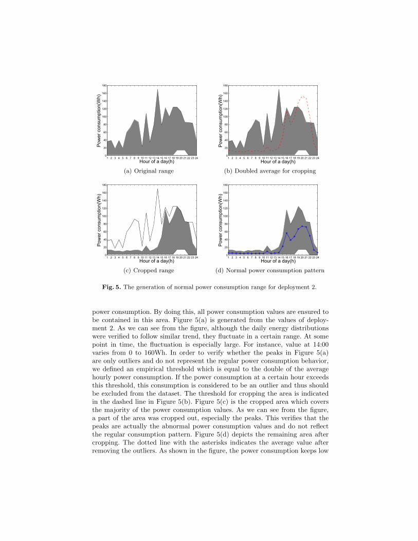
In order to filter out abnormal power consumption behavior, we extracted theminimum and maximum power consumption of each hour over the whole deploy-ment. Using these values we formed an area as shown in Figure 5(a) where thex axis represents the hour of the day, and the y axis represents the associated

1 2 3 4 5 6 7 8 9 10 11 12 13 14 15 16 17 18 19 20 21 22 23 240

20

40

60

80

100

120

140

160

180

Hour9of9a9day(h)

Pow

er9c

onsu

mpt

ion(

Wh)

Hour9of9a9day(h)

Pow

er9c

onsu

mp

tion(

Wh)

(a) Original range

1 2 3 4 5 6 7 8 9 10 11 12 13 14 15 16 17 18 19 20 21 22 23 240

20

40

60

80

100

120

140

160

180

Hour9of9a9day(h)

Pow

er9c

onsu

mpt

ion(

Wh)

Hour9of9a9day(h)

Pow

er9c

onsu

mp

tion(

Wh)

(b) Doubled average for cropping

1 2 3 4 5 6 7 8 9 10 11 12 13 14 15 16 17 18 19 20 21 22 23 240

20

40

60

80

100

120

140

160

180

Hour9of9a9day(h)

Pow

er9c

onsu

mpt

ion(

Wh)

Hour9of9a9day(h)

Pow

er9c

onsu

mp

tion(

Wh)

(c) Cropped range

1 2 3 4 5 6 7 8 9 10 11 12 13 14 15 16 17 18 19 20 21 22 23 240

20

40

60

80

100

120

140

160

180

Hour9of9a9day(h)

Pow

er9c

onsu

mpt

ion(

Wh)

Hour9of9a9day(h)

Pow

er9c

onsu

mp

tion(

Wh)

(d) Normal power consumption pattern

Fig. 5. The generation of normal power consumption range for deployment 2.

power consumption. By doing this, all power consumption values are ensured tobe contained in this area. Figure 5(a) is generated from the values of deploy-ment 2. As we can see from the figure, although the daily energy distributionswere verified to follow similar trend, they fluctuate in a certain range. At somepoint in time, the fluctuation is especially large. For instance, value at 14:00varies from 0 to 160Wh. In order to verify whether the peaks in Figure 5(a)are only outliers and do not represent the regular power consumption behavior,we defined an empirical threshold which is equal to the double of the averagehourly power consumption. If the power consumption at a certain hour exceedsthis threshold, this consumption is considered to be an outlier and thus shouldbe excluded from the dataset. The threshold for cropping the area is indicatedin the dashed line in Figure 5(b). Figure 5(c) is the cropped area which coversthe majority of the power consumption values. As we can see from the figure,a part of the area was cropped out, especially the peaks. This verifies that thepeaks are actually the abnormal power consumption values and do not reflectthe regular consumption pattern. Figure 5(d) depicts the remaining area aftercropping. The dotted line with the asterisks indicates the average value afterremoving the outliers. As shown in the figure, the power consumption keeps low

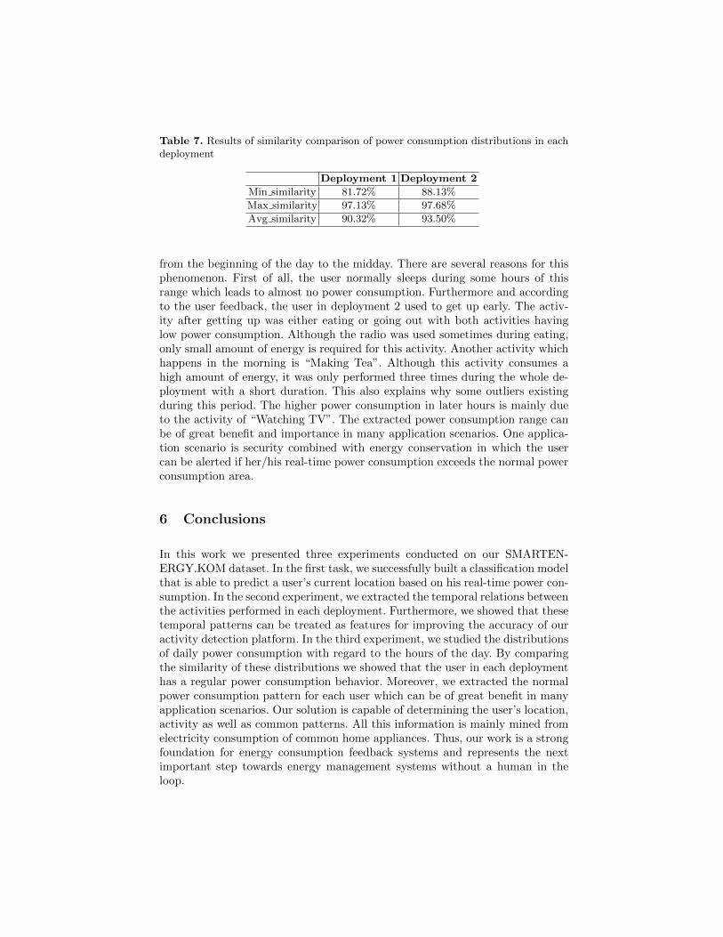
Table 7. Results of similarity comparison of power consumption distributions in eachdeployment

Deployment 1 Deployment 2

Min similarity 81.72% 88.13%

Max similarity 97.13% 97.68%

Avg similarity 90.32% 93.50%

from the beginning of the day to the midday. There are several reasons for thisphenomenon. First of all, the user normally sleeps during some hours of thisrange which leads to almost no power consumption. Furthermore and accordingto the user feedback, the user in deployment 2 used to get up early. The activ-ity after getting up was either eating or going out with both activities havinglow power consumption. Although the radio was used sometimes during eating,only small amount of energy is required for this activity. Another activity whichhappens in the morning is “Making Tea”. Although this activity consumes ahigh amount of energy, it was only performed three times during the whole de-ployment with a short duration. This also explains why some outliers existingduring this period. The higher power consumption in later hours is mainly dueto the activity of “Watching TV”. The extracted power consumption range canbe of great benefit and importance in many application scenarios. One applica-tion scenario is security combined with energy conservation in which the usercan be alerted if her/his real-time power consumption exceeds the normal powerconsumption area.

6 Conclusions

In this work we presented three experiments conducted on our SMARTEN-ERGY.KOM dataset. In the first task, we successfully built a classification modelthat is able to predict a user’s current location based on his real-time power con-sumption. In the second experiment, we extracted the temporal relations betweenthe activities performed in each deployment. Furthermore, we showed that thesetemporal patterns can be treated as features for improving the accuracy of ouractivity detection platform. In the third experiment, we studied the distributionsof daily power consumption with regard to the hours of the day. By comparingthe similarity of these distributions we showed that the user in each deploymenthas a regular power consumption behavior. Moreover, we extracted the normalpower consumption pattern for each user which can be of great benefit in manyapplication scenarios. Our solution is capable of determining the user’s location,activity as well as common patterns. All this information is mainly mined fromelectricity consumption of common home appliances. Thus, our work is a strongfoundation for energy consumption feedback systems and represents the nextimportant step towards energy management systems without a human in theloop.

7 Acknowledgments

This work has been financially supported by the German Research Foundation(DFG) in the framework of the Excellence Initiative, Darmstadt Graduate Schoolof Excellence Energy Science and Engineering (GSC 1070) and has been co-funded by the Social Link Project within the Loewe Program of Excellence inResearch, Hessen, Germany.

References

1. R. Agrawal, R. Srikant, et al. Fast algorithms for mining association rules. 1994.2. A. Alhamoud, F. Ruettiger, A. Reinhardt, F. Englert, D. Burgstahler, D. Bohn-

stedt, C. Gottron, and R. Steinmetz. Smartenergy.kom: An intelligent systemfor energy saving in smart home. In Local Computer Networks Workshops (LCNWorkshops), 2014 IEEE 39th Conference on, pages 685–692, Sept 2014.

3. J. F. Allen and G. Ferguson. Actions and events in interval temporal logic. Journalof logic and computation, 4(5):531–579, 1994.

4. C. Chen, D. J. Cook, and A. S. Crandall. The user side of sustainability: Mod-eling behavior and energy usage in the home. Pervasive and Mobile Computing,9(1):161–175, 2013.

5. F. Englert, T. Schmitt, S. Koessler, A. Reinhardt, and R. Steinmetz. How to auto-configure your smart home?: High-resolution power measurements to the rescue.In Proceedings of the Fourth International Conference on Future Energy Systems,e-Energy ’13, pages 215–224, New York, NY, USA, 2013. ACM.

6. J. Fogarty, C. Au, and S. E. Hudson. Sensing from the basement: a feasibility studyof unobtrusive and low-cost home activity recognition. In Proceedings of the 19thannual ACM symposium on User interface software and technology, pages 91–100.ACM, 2006.

7. M. Hall, E. Frank, G. Holmes, B. Pfahringer, P. Reutemann, and I. H. Witten.The WEKA data mining software: an update. SIGKDD Explor.Newsl., 11(1):10–18, Nov. 2009.

8. E. Hoque and J. Stankovic. AALO: Activity recognition in smart homes usingactive learning in the presence of overlapped activities. In Pervasive ComputingTechnologies for Healthcare (PervasiveHealth), 6th International Conference on,pages 139–146. IEEE, 2012.

9. Z. C. Johanyak and S. Kovacs. Distance based similarity measures of fuzzy sets.Proceedings of SAMI, 2005.

10. E. Keogh and C. A. Ratanamahatana. Exact indexing of dynamic time warping.Knowledge and information systems, 7(3):358–386, 2005.

11. W. Kleiminger, C. Beckel, T. Staake, and S. Santini. Occupancy detection fromelectricity consumption data. In Proceedings of the 5th ACM Workshop on Em-bedded Systems For Energy-Efficient Buildings, BuildSys’13, pages 10:1–10:8, NewYork, NY, USA, 2013. ACM.

12. R. Kohavi et al. A study of cross-validation and bootstrap for accuracy estimationand model selection. In IJCAI, volume 14, pages 1137–1145, 1995.

13. J. Lin, E. Keogh, S. Lonardi, and B. Chiu. A symbolic representation of timeseries, with implications for streaming algorithms. In Proceedings of the 8th ACMSIGMOD workshop on Research issues in data mining and knowledge discovery,pages 2–11. ACM, 2003.

14. B. Liu, Y. Ma, and C.-K. Wong. Classification using association rules: weaknessesand enhancements. In Data mining for scientific and engineering applications,pages 591–605. Springer, 2001.

15. D. Lymberopoulos, A. Bamis, and A. Savvides. Extracting spatiotemporal humanactivity patterns in assisted living using a home sensor network. Universal Accessin the Information Society, 10(2):125–138, 2011.

16. A. Reinhardt, P. Baumann, D. Burgstahler, M. Hollick, H. Chonov, M. Werner,and R. Steinmetz. On the accuracy of appliance identification based on distributedload metering data. In Sustainable Internet and ICT for Sustainability, 2012, pages1–9, Oct 2012.