Extinction-to-backscatter Ratios of Saharan Dust Layers Derived from 1

In-Situ Measurements and CALIPSO Overflights during NAMMA 2

3

A. H. Omar, Z. Liu, M. Vaughan, K. L. Thornhill, C. Kittaka, S. Ismail, Y. Hu, G. Chen, 4 K. Powell, D. Winker, C. Trepte, E. L. Winstead, B. E Anderson 5

Abstract 6

We determine the extinction-to-backscatter (Sa) ratios of dust using (1) airborne in-situ 7

measurements of microphysical properties, (2) modeling studies, and (3) the Cloud-8

Aerosol Lidar and Infrared Pathfinder Satellite Observations (CALIPSO) observations 9

recorded during the NASA African Monsoon Multidisciplinary Analyses (NAMMA) 10

field experiment conducted from Sal, Cape Verde during Aug-Sept 2006. Using 11

CALIPSO measurements of the attenuated backscatter of lofted Saharan dust layers, we 12

apply the transmittance technique to estimate dust Sa ratios at 532 nm and a 2-color 13

method to determine the corresponding 1064 nm Sa. This method yielded dust Sa ratios of 14

39.8 ± 1.4 sr and 51.8 ± 3.6 sr at 532 nm and 1064 nm, respectively. Secondly, Sa at both 15

wavelengths is independently calculated using size distributions measured aboard the 16

NASA DC-8 and estimates of Saharan dust complex refractive indices applied in a T-17

Matrix scheme. We found Sa ratios of 39.1 ± 3.5 sr and 50.0 ± 4 sr at 532 nm and 1064 18

nm, respectively, using the T-Matrix calculations applied to measured size spectra. 19

Finally, in situ measurements of the total scattering (550 nm) and absorption coefficients 20

(532 nm) are used to generate an extinction profile that is used to constrain the CALIPSO 21

532 nm extinction profile and thus generate a stratified 532 nm Sa. This method yielded 22

an Sa ratio at 532 nm of 35.7 sr in the dust layer and 25 sr in the marine boundary layer 23

consistent with a predominantly seasalt aerosol near the ocean surface. Combinatorial 24

simulations using noisy size spectra and refractive indices were used to estimate the mean 25

and uncertainty (one standard deviation) of these Sa ratios. These simulations produced a 26

mean (± uncertainty) of 39.4 (± 5.9) sr and 56.5 (± 16.5) sr at 532 nm and 1064 nm, 27

respectively, corresponding to percent uncertainties of 15% and 29%. These results will 28

provide a measurements-based estimate of the dust Sa for use in backscatter lidar 29

inversion algorithms such as CALIOP. 30

2

1. Introduction 31

Lidar is a powerful tool for studying the vertical distribution of aerosols and clouds in the 32

atmosphere. Of particular importance is the distribution and transport of Saharan dust 33

systems. The deployment of CALIPSO (Cloud-Aerosol Lidar and Infrared Pathfinder 34

Satellite Observations), a joint NASA-CNES satellite mission, has enabled vertically 35

resolved measurements of Sahara air layer(s) (SAL) which will provide significant 36

insights into properties of Sahara dust aerosols. CALIPSO is designed to provide 37

measurements to advance our understanding of the role of aerosols and clouds in the 38

climate system [Winker et al., 2009]. The Cloud-Aerosol LIdar with Orthogonal 39

Polarization [CALIOP, Winker et al., 2007] is the primary instrument on the CALIPSO 40

satellite. CALIOP is designed to acquire vertical profiles of elastic backscatter at two 41

wavelengths (1064 nm and 532 nm) from a near nadir-viewing geometry during both day 42

and night phases of the orbit. In addition to the total backscatter at the two wavelengths, 43

CALIOP also provides profiles of linear depolarization at 532 nm. Accurate aerosol and 44

cloud heights and retrievals of extinction coefficient profiles are derived from the total 45

backscatter measurements [Vaughan et al., 2009] The depolarization measurements 46

enable the discrimination between ice clouds and water clouds [Hu et al., 2009] and the 47

identification of non-spherical aerosol particles [Liu et al., 2009]. Additional information, 48

such as estimates of particle size for the purpose of discriminating between clouds and 49

aerosols, are obtained from the ratios of the signals obtained at the two wavelengths. On 50

April 28, 2006, the CALIPSO satellite was launched into a low earth sun-synchronous 51

orbit at a 705-km altitude, and an inclination of 98.2 degrees. A few months later, in 52

August 2006, the NASA African Monsoon Multidisciplinary Analyses (NAMMA) 53

3

campaign commenced at the Cape Verde Islands, 350 miles off the coast of Senegal in 54

West Africa. NAMMA was designed to study the evolution of precipitating convective 55

systems, largely as this evolution pertained to the SAL and its role in the tropical 56

cyclogenesis. Several aircraft flights were dedicated to nearly coincident measurements 57

with NASA’s orbiting satellites (including Aqua, TRMM, and CloudSat/CALIPSO). For 58

this study, we use data collected aboard NASA's DC-8 medium altitude research aircraft 59

outfitted with, among other instruments, a full suite of sensors and probes designed to 60

measure aerosol microphysical and optical properties. Relevant parameters include high 61

spatial-resolution scattering and absorption coefficients at multiple wavelengths in the 62

visible spectrum and dry particle size distributions over the 0.08 to 10 m diameter range 63

[Chen et al., 2010]. 64

Depending on the mineralogical composition, the SAL can have a significant impact on 65

both the radiation balance and cloud processes. Dust particles scatter in the shortwave 66

regime (cooling the planet) and absorb both shortwave and longwave radiation (heating 67

the planet). By some estimates the anthropogenic forcing due to dust is comparable to the 68

forcing by all other anthropogenic aerosols combined [Sokolik and Toon, 1996]. Saharan 69

dust influences cyclone activity and convection in the region off the west coast of Africa 70

and air quality as far west as the US east coast and Gulf of Mexico. There have been 71

reports of causal links between cyclone activity and dust loading suggesting that perhaps 72

the Sahara dust layer acts to inhibit cyclone development [Dunion and Velden, 2004] and 73

more generally convection [Wong and Dessler, 2005]. Sahara dust is unique in its ability 74

to maintain layer integrity as it is transported over long distances (~7500 km) to the 75

Americas [Liu et al., 2008; Maring et al., 2003; Savoie and Prospero, 1976]. The 76

4

presence of Sahara dust layers have been found to perturb ice nuclei (IN) concentrations 77

as far away as in Florida. During CRYSTAL-FACE (Cirrus Regional Study of Tropical 78

Anvils and Cirrus Layers - Florida Area Cirrus Experiment), DeMott et al. [2003] found 79

that IN concentrations were significantly enhanced in heterogeneous ice nucleation 80

regimes warmer than -38°C, when Saharan dust layers are present. It is therefore 81

important to study the distribution and optical properties of Sahara dust. 82

In order to estimate the optical depth of the Sahara dust layers from elastic backscatter 83

lidar measurements, the Sa ratio must be known or prescribed. Given aerosol free regions 84

above and below a lofted dust aerosol layer, Sa can be calculated from the attenuated 85

backscatter profile of a space-based lidar return [Young, 1995]. Sa for dust aerosols is 86

dependent on the mineral composition, size distribution, and shape parameters (e.g., 87

aspect ratio, and complexity factor). All of these are highly variable and for the most part 88

not well known. For these reasons, Sa obtained from scattering models have larger 89

uncertainties than models of the nearly spherical urban pollution or marine aerosols. 90

There have been several studies and measurements of dust Sa at 532 nm [Ackermann, 91

1998; Anderson et al., 2000; Berthier et al., 2006; Di Iorio et al., 2003; Di Iorio et al., 92

2009; Muller et al., 2007; Müller et al., 2000; Tesche et al., 2009] and relatively few such 93

measurements or studies of dust Sa at 1064 nm [Ackermann, 1998; Liu et al., 2008; 94

Tesche et al., 2009]. Prior to NAMMA, there were a number of vertically-resolved 95

measurements of Saharan dust microphysical and optical properties including AMMA 96

and DODO campaigns NAMMA studies along with CALIPSO measurements provide a 97

unique opportunity to compare extinction measurements derived from in situ profile 98

measurements of total scattering and absorption aboard the NASA DC-8 and CALIPSO 99

5

extinction profiles estimated from two wavelength retrieval methods. These profiles by 100

extension provide the constraints from which the lidar ratios can be determined as 101

explained in the following sections. Section 2 discusses the CALIPSO lidar data and its 102

analysis. The NAMMA data and analyses are discussed in Section 3, and coincident 103

CALIPSO-NAMMA measurements are presented in Section 4. In Section 5, the size 104

distributions measured during NAMMA aboard the DC-8 are implemented in a T-Matrix 105

scheme to estimate profiles of Sa ratios. Section 6 discusses the uncertainty in Sa using a 106

combinatorial method. 107

108

2. CALIPSO Lidar Data and Extinction-to-Backscatter Ratio Retrieval 109

Methods 110

The CALIPSO lidar data used for these studies are the version 2.01 lidar level 1 111

attenuated backscatter returns at the 532 nm perpendicular and parallel channels, and 112

1064 nm total attenuated backscatter. The volume depolarization ratio is determined from 113

the perpendicular and parallel channels and used to identify dust aerosols [Liu et al., 114

2009; Omar et al., 2009]. For NAMMA underflights of CALIPSO and near spatial 115

coincidences where both missions observed dust layers of optical depths greater than 116

about 0.3, we compare the extinction profiles from in situ measurements to CALIPSO 117

profiles. In such cases, we calculate the extinction using Sa that was determined using the 118

transmittance method or an Sa ratio constrained by the in-situ extinction profiles. In both 119

cases, we use the 2-color methods to retrieve the 1064-nm Sa, after determining the 532-120

nm Sa. These two methods, transmittance and 2-color, are discussed below. 121

6

2.1. Transmittance Methods 122

The transmittance method uses the following equation describing the relationship 123

between optical depth and integrated attenuated backscatter, as in Platt [1973]: 124

125

a

11 exp 2

2 S

(1) 126

127

Here is the integrated (from layer base to top) attenuated backscatter, 128

129

top2

a abase

(r)T (r)dr (2) 130

131

is optical depth, is a multiple scattering parameter, T2 = exp(-2) is the layer-132

effective two-way transmittance, and Sa = σa/βa where βa is the aerosol backscatter 133

coefficient and σa is the aerosol extinction coefficient. This ratio is assumed constant 134

throughout a feature. Note that the quantities Sa, ', and describe characteristics of an 135

aerosol layer, i.e., they are associated with the backscatter and extinction of aerosol 136

particles only. If we define an effective Sa ratio, S* = Sa, we can rewrite Eq. (1) as 137

follows: 138

21 TS*

2

(3) 139

140

The effective two-way transmittance is typically obtained by fitting the returns both 141

above and below a feature to a reference clear air scattering profile obtained from local 142

7

rawinsonde measurements or meteorological model data [Young, 1995]. In this study, the 143

transmittance method is used to determine S* from the 532-nm CALIPSO measurements 144

whenever clear air scattering signals are available both above and below an aerosol layer. 145

However, the same method is not applicable to the 1064-nm CALIPSO measurements, 146

because a reliable measurement of the clear air scattering at 1064 nm, which is about 16 147

times smaller than that at 532 nm, is not available. To determine S* at 1064 nm, the 2-148

color method described in the next subsection is used. 149

150

2.2. The 2-Color Method 151

The 2-color or two-wavelength method was first proposed by Sasano and Browell 152

[Sasano and Browell, 1989] and adapted to space-borne lidar measurements using an 153

optimization technique by Vaughan et al. [2004]. The method requires apriori knowledge 154

of Sa at 532 nm and a suitable profile of 532-nm attenuated backscatter amenable to the 155

calculation of 532-nm aerosol backscatter coefficient profiles. For the NAMMA cases 156

described below these preconditions were satisfied. Whenever a suitable region of clear 157

air was identified both above and below an aerosol layer, the Sa at 532 nm was 158

determined using the transmittance method described above. Here clear air layer is 159

defined as a region of low attenuated scattering ratios with a mean value equal to or less 160

than 1 and a slope with respect to altitude of approximately zero. This is further 161

confirmed by low volume depolarization ratios in a small region (~ 1/2 km) below the 162

aerosol layer. In cases where coincident NAMMA measurements are available, Sa ratio at 163

532 nm is the value that provides the best fit between the retrieved CALIPSO extinction 164

profiles and the NAMMA in situ extinction profiles obtained by summing the total 165

8

scattering and absorption measured by a nephelometer and a Particle Soot/Absorption 166

Photometer (PSAP), respectively, aboard the DC-8. 167

168

Once Sa ratio is determined at 532 nm, the value at 1064 nm can be calculated using the 169

2-color method. We note that this technique can be used to derive Sa at 532 nm if the 170

value at 1064 nm is known. Given a solution of the particulate backscatter at 532 nm, 171

β532,p, the 2-color method uses a least squares method to minimize the difference between 172

the measured attenuated total backscatter at 1064 nm, B1064, and the attenuated 173

backscatter at 1064 nm (right hand side of eq. (4)) reconstructed from the extinction and 174

backscatter coefficients at 532 nm. 175

176

1064

m,1064 p,532 1064 532

2m,1064 p,1064 p,1064B r r T r

r r exp 2 S r

(4) 177

178

The only unknowns (underlined) in eq.(4), are the Sa ratio at 1064 nm, S1064, and the 179

backscatter color ratio, χ (defined as β1064,p/β532,p). These are both intensive aerosol 180

properties defined by the layer composition, size distribution, and shape of its constituent 181

particles. Since these characteristics do not vary substantially in a given aerosol layer, we 182

make the assumption that S1064 and χ are constant within the layer. The algorithm details 183

and optimization techniques are discussed at length in Vaughan (2004) and Vaughan et 184

al. [2004] 185

9

3. Numerical Calculation Based on NAMMA In-situ Measurements 186

3.1. Aerosol Microphysical Properties 187

We use measurements of the aerosol size distributions based on number from the 188

Aerodynamic Particle Sizer (APS, TSI Incorporated, Shoreview, MN) and the Ultra-High 189

Sensitivity Aerosol Spectrometer (UHSAS, Droplet Measuring Systems, Boulder, CO). 190

The UHSAS measures the fine mode aerosol size distributions from 0.06 to 0.98 μm, and 191

the APS measures the coarse mode size distributions from 0.6 to 5.5 μm. We use the size 192

distributions to identify the presence of aerosol dust layers. In many cases, these intense 193

dust layers were visually identified by the instrument operators and in some cases 194

specifically targeted by the DC-8 operators for sampling. Additional information about 195

the composition of these layers is available from the NAMMA data archives 196

(http://namma.msfc.nasa.gov/). For each size distribution sampled during a 5-second 197

interval we fit the discrete measurements to the best continuous bimodal lognormal size 198

distribution, as shown in Figure 1. The geometric mean radius and standard deviation of a 199

fine and coarse mode derived from the in situ measurements are used in the numerical 200

calculations. 201

202

On August 25, 2008, the DC-8 flew through a dense elevated dust layer measuring nearly 203

1 km in thickness at a mean altitude of about 2.3 km in an hour-long mostly straight and 204

level flight. The APS and UHSAS measured coarse and fine size distributions, 205

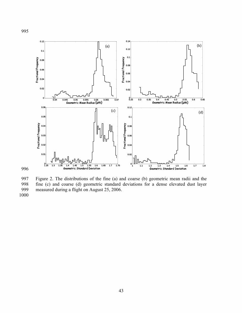
respectively, through the dust layer at intervals of 5 seconds. Figure 2 shows the 206

probability distributions of the geometric mean fine and coarse radii of the dust layer. 207

This figure is generated by taking the discrete 5-second size distribution measurements 208

10

and fitting these to a bimodal lognormal distribution as described above. For this dust 209

layer, the microphysical properties of mean, median, and standard deviations of the fine 210

(coarse) radius distributions, as shown in Figures 2 (a) and (b), are 0.059, 0.061, and 211

0.0064 μm (0.54, 0.57, and 0.083 μm), respectively. The mean, median, and standard 212

deviations shown in Figure 2 (c) and (d) for the fine (coarse) geometric standard 213

deviation distributions are 1.613, 1.630, and 0.101 (1.495, 1.545, and 0.151), 214

respectively. 215

216

The distributions in Figure 2 show that dust properties after lofting of these layers remain 217

relatively unchanged. Other studies [Liu et al., 2008; Maring et al., 2003; Prospero and 218

Carlson, 1971; 1972], have shown the same consistency in properties after long range 219

transport of dust. In each case, the means and medians of the size distribution descriptors 220

are close, i.e., the size descriptors are nearly normally distributed. The standard deviation 221

is a small fraction (<0.16) of the means, i.e., the variance of the data is small and thus the 222

layer is quite homogenous with respect to size across the 1 km vertical extent of the dust 223

plume. 224

225

3.2. Scattering Models 226

Mie scattering calculations [Mie, 1908], when applied to dust, are adequate for total 227

scattering, albedo and other flux related quantities, but result in large errors when used to 228

retrieve optical depth from satellite reflectance measurements. In particular and central to 229

the theme of this paper, are Sa ratios calculated from measured size distributions. Mie 230

calculations underestimate Sa by up to a factor of 2.0 leading to substantial errors in the 231

11

lidar derived aerosol optical depths [Kalashnikova and Sokolik, 2002]. This has been 232

known experimentally for quite some time: laboratory measurements by Perry et al 233

[1978] showed non-spherical particles, when compared to spherical particles having the 234

same equivalent volume, enhance side scattering and suppress backscattering. To account 235

for non-sphericity of dust particles, we use T-matrix calculations with the assumption that 236

the dust shapes can be modeled by randomly oriented prolate spheroids. T-Matrix is a 237

matrix formulation of electromagnetic scattering first proposed by Waterman [1971], and 238

subsequently improved and extended to much larger sizes and aspect ratios by Mischenko 239

et al. in a series of papers [Mishchenko, 1991; 1993; Mishchenko and Travis, 1994; 240

Mishchenko et al., 1996a; Mishchenko et al., 1996b; Mishchenko and Travis, 1998]. The 241

T-Matrix code used in these calculations is described in detail in Mishchenko and Travis 242

[1998]. This method is particularly suitable for light scattering calculations of non-243

spherical, polydisperse, randomly oriented particles of identical axially symmetric shape 244

with size parameter, x (x= πdp/λ; dp is particle diameter and λ is the wavelength), smaller 245

than 30. 246

247

It is challenging to determine representative statistics of the mean shape for dust particles 248

because of their complexity and variety in shape. These particles are not only confined to 249

desert regions but are ubiquitous in continental areas where they contribute quite 250

significantly to the extinction budget [Omar et al., 1999]. Fortunately, however, 251

randomly oriented prolate and oblate spheroids can adequately represent the scattering 252

properties of non-spherical particles of the same aspect ratio [cf. Mischenko et al., 1995; 253

Mishchenko and Travis, 1994]. The aspect ratio is the ratio of the largest to the smallest 254

12

particle dimension. A prolate (oblate) spheroid is a rotationally symmetric ellipsoid with 255

a polar diameter greater (smaller) than the equatorial diameter. 256

257

There have been several studies of aspect ratio distributions representative of dust 258

aerosols. From an analysis of scanning electron microscope images of yellow sand 259

particles, Nakajima et al. [1989] found that the distribution of the minor to major particle 260

radius ratio peaked around 0.6, equivalent to an aspect ratio of 1.67. An investigation of 261

mineral dust particle shapes using electron microscopy by Okada et al. [1987] found a 262

mean aspect ratio of 1.4 ranging from 1.0 to 2.3. Hill et al [1984] compared the measured 263

scattering properties of 312 samples of soil dust with the simulated scattering properties 264

of randomly oriented prolate spheroids using T-matrix. They found the distributions of 265

the aspect ratio of prolate spheroids centered near 2.3 most closely reproduced the 266

measured scattering properties. For this study, we use a mean aspect ratio of 2.0 based on 267

the above studies and investigate the sensitivity of the Sa ratio to aspect ratios ranging 268

from 1.7 to 2.3 partly to account for the dependence of the aspect ratio on size as 269

discussed by Kalashnikova and Sokolik [2004]. 270

271

There is quite a wide range of estimated and measured mineral dust refractive indices (m-272

ik). For wavelengths of 550 and 1000 nm, d’Almeida et al. [1991] estimate the real part 273

(m) of 1.53 and 1.52, respectively, and a spectrally invariant imaginary part (k) of 0.008 274

for dust-like aerosols, and 1.53-i0.0055 and 1.53-i0.001, respectively, for mineral dust. 275

Ackerman (1998) used values of 1.53-i0.0043 and 1.53-i0.0063 to calculate dust Sa ratios 276

of 19-23 sr and 17-18 sr at 532 and 1064 nm, respectively. These values are much lower 277

13

than more recent 532-nm dust Sa ratios of 40-60 sr [Cattrall et al., 2005; Di Iorio et al., 278

2003; Muller et al., 2007; Murayama et al., 2003; Voss et al., 2001] because the 279

Ackerman study assumed spherical particles. 280

Retrievals from radiances measured by ground-based Sun-sky scanning radiometers of 281

the Aerosol Robotic Network (AERONET) over a 2-year period yielded dust complex 282

refractive index values of 1.55 ± 0.03 – i0.0014 ± 0.001 at 670 nm and 1.55 ± 0.03-i0.001 283

± 0.001 at 1020 nm at Bahrain (Persian Gulf), and 1.56 ± 0.03 – i0.0013 ± 0.001 at 670 284

nm and 1.56 ± 0.03-i0.001 ± 0.001 at 1020 nm at Solar Village in Saudi Arabia [Dubovik 285

et al., 2002]. Using vertically resolved aerosol size distributions in a scattering model 286

constrained by lidar measurements of aerosol backscattering coefficient at 532 nm, Di 287

Iorio et al. (2003) estimated dust refractive indices of 1.52 to 1.58 (real part), and 0.005 288

to 0.007 (imaginary part). Kalashnikova and Sokolik [2004] calculated effective 289

refractive indices from component mixtures and found values of 1.61-i0.0213 and 1.59-290

i0.0032 for Saharan dust at wavelengths of 550 nm and 860 nm, respectively. The values 291

for Asian dust, from the same monograph, are 1.51-i0.0021 and 1.51-i0.0007 at 550 nm 292

and 860 nm, respectively. Using a twin angle optical counter , Eidehammer et al.(2008) 293

estimated the indices of refraction to be in the range 1.60-1.67 for the real part and 0.009-294

0.0104 for the imaginary part. 295

296

The Saharan Mineral Dust Experiment [SAMUM, Heintzenberg, 2009; Rodhe, 2009] 297

based in Morocco in 2006, produced several independent estimates of the complex 298

refractive indices of Saharan dust. Kandler et al. [2009] determined Saharan dust aerosol 299

complex refractive index from chemical/mineralogical composition of 1.55-i0.0028 and 300

14

1.57-i0.0037 at 530 nm for small (diameter < 500 nm) and large particles (diameter > 500 301

nm), respectively. Schladitz et al. [2009] derived mean refractive indices of 1.53 - 302

i0.0041 at 537 nm and 1.53 - i0.0031at 637 nm from measurements of scattering and 303

absorption coefficients, and particle size distributions. Using similar methods during 304

SAMUM, Petzold et al. [2009] found real parts of the refractive indices of Saharan dust 305

ranging from 1.55 to 1.56 and imaginary parts ranging from 0.0003 to 0.0052. Some of 306

the estimates of refractive indices reported in the literature are summarized in Table 1. 307

308

15

Table 1. Summary of complex dust refractive indices from previous studies 309

Wavelength

(nm)

Real Part Imaginary Part Source

500 1.50 0.0045 Volz [1973]

1000 1.53 0.008 d’Almeida et al. [1991], dust-like

550 1.53 0.0055 d’Almeida et al. [1991], mineral dust

1000 1.53 0.001 d’Almeida et al. [1991], mineral dust

532 1.53 0.0043 Ackerman [1998] dust

1064 1.53 0.0063 Ackerman [1998] dust

670 1.55 ± 0.03 0.0014 ± 0.001 Dubovik et al. [2002], Bahrain dust

1020 1.55 ± 0.03 0.003 ± 0.001 Dubovik et al. [2002], Bahrain dust

670 1.56 ± 0.03 0.0013 ± 0.001 Dubovik et al. [2002], Solar Village dust

1020 1.56 ± 0.03 0.001 ± 0.001 Dubovik et al. [2002], Solar Village dust

532 1.52-1.58 0.005-0.007 Di Iorio et al. [2003], Saharan dust

500 1.42 0.003 Israelevich [2003], Sede Boker dust

860 1.51 0.0032 Kalashnikova and Sokolik [2004] Saharan dust

550 1.51 0.002 Kalashnikova and Sokolik [2004] Asian dust

860 1.51 0.0007 Kalashnikova and Sokolik [2004] Asian dust

670 1.45 0.0036 Omar et al. [2005] dust cluster

550 1.53 0.0015 Cattrall et al.[2005] mineral dust

1020 1.53 0.0005 Cattrall et al. [2005] mineral dust

300-700 1.60-1.67 0.009-0.0104 Eidehammer et al. [2008] Wyoming dust

537 1.53 0.0041 Schladitz et al. [2009] Saharan dust

637 1.53 0.0031 Schladitz et al. [2009] Saharan dust

450 1.55-1.56 0.0003-0.0052 Petzold et al. [2009] Saharan dust

700 1.55-1.56 0.0003-0.0025 Petzold et al. [2009] Saharan dust

530 1.55 0.0028-0.0037 Kandler et al. [2009] Saharan dust

310

To perform the sensitivity study described in section 6, we use values of the real part of 311

the refractive index ranging from 1.45 – 1.55 (normally distributed) and the imaginary 312

16

part ranging from 0.00067 – 0.006 (log normally distributed) with a central value of 1.50-313

i0.002. For the scattering calculations using NAMMA size distributions, we use the 314

central values of the refractive indices along with the nearly instantaneous (5 second 315

interval) size distribution measurements to generate profiles of the aerosol properties. 316

Figure 3 is a plot of the fine mode, coarse mode, and total phase function of the dust 317

plume encountered on August 19, 2006. The fine mode and coarse mode phase functions 318

are computed from the mean of the instantaneous size distributions, and the total phase 319

function is the area-weighted composite of the fine and coarse mode phase functions. The 320

phase functions are driven largely by the coarse mode, especially at 532 nm, and exhibit a 321

more pronounced peak in the backscattering direction at 532 nm than 1064 nm 322

323

4. Data Analyses of CALIPSO NAMMA Coincident Measurements 324

For this study we analyzed coincident measurements of the CALIOP 532-nm extinction 325

profiles and in situ extinction profiles measured at wavelengths near the CALIOP green 326

channel. The in situ extinction coefficient is obtained by summing the scattering (550 327

nm) and absorption (532 nm) coefficients measured by a nephelometer and a PSAP, 328

respectively. Data from the nephelometer and PSAP have been corrected for errors 329

associated with the limited detector viewing angle [Anderson and Ogren, 1998] and 330

scattering from the filter media [Virkkula et al., 2005], respectively. We make the 331

assumption that the scattering properties are invariant over the 532 – 550 nm range for 332

these large dust particle sizes. We chose three days on which there were near collocated 333

CALIPSO and NAMMA measurements of nearly the same airmass. 334

17

4.1. August 19, 2006 NAMMA Flight 4 335

August 19 was one of the days the DC-8 performed an under flight of CALIPSO. Figure 336

4 shows the time-altitude flight track of the DC-8. A nearly coincident in-situ profile was 337

obtained during the second ascent leg shown in the figure. Atmospheric context for this 338

flight is given by Figure 5(a) and (b), in which both the DC-8 and CALIPSO flight tracks 339

are superimposed on images of measurements made by the Moderate Resolution Imaging 340

Spectroradiometer (MODIS) and Measurements of Pollution in the Troposphere 341

(MOPITT), respectively. The DC-8 flight tracks are the black irregular octagons and the 342

CALIPSO orbit tracks are the straight lines in both images. The underflights in the 343

figures are segments where the DC-8 flight tracks are nearly exactly collocated and 344

parallel to the CALIPSO flight tracks. The MODIS optical depth near the coincident 345

flight segment is about 0.5. The MOPPITT image shows moderate CO concentrations in 346

the vicinity of the coincident flight track and therefore indicates that most of the aerosol 347

is dust and not continental pollution or biomass burning. This can also be confirmed by 348

the CALIPSO depolarization measurements. The image also shows high CO 349

concentrations (>2.5x1018 molecules/cm2) to the south of the DC-8 flight tracks most 350

likely due to biomass burning, and identified as such by the CALIPSO aerosol subtyping 351

scheme illustrated later in this section. 352

353

Unfortunately, the direct underflight of CALIPSO by the DC-8 was a nearly level flight 354

with no in situ profile information. In fact the DC-8 was at a high altitude near Flight 355

Level 330 (~ 10 km) throughout the underflight and therefore did not encounter any 356

significant aerosol layer at this altitude to sample. We used the ascending leg of the DC-8 357

18

flight which corresponds to the flight segment during ascent to the CALIPSO underflight 358

portion denoted by blue dots in Fig 5a. The in situ profiles segment is shown in Fig. 4. 359

The CALIPSO browse images (e.g., Fig. 6) are plots of the attenuated backscatter color 360

coded by intensity varying from blue (weak) to white (very strong). A horizontal line 361

near the 0 km mark denotes the surface. The CALIPSO data used for comparison with the 362

in-situ data come from the 80 profiles (~27 km horizontal average) between the white 363

lines in the browse image (Fig. 6). To determine the optimal 532-nm Sa ratio for these 364

data, we iteratively adjust Sa until the difference, in a least squares sense, between the 365

retrieved CALIPSO profile, σa,532-nm, and the measured NAMMA profile, σa,550-nm, is 366

minimized. 367

368

Figure 7 is a plot of the extinction profiles retrieved from CALIPSO’s 532-nm 369

backscatter profiles and the profiles of the sum of scattering (550 nm) and absorption 370

(532 nm) measured by the nephelometer and the PSAP aboard the NASA DC-8, 371

respectively. These profiles were taken during the ascent leg shown in Figure 4 372

corresponding to the flight tracks shown in Figure 5(a). The boundary between the two 373

layers is determined by the increase in the extinction coefficient near 2 km. The two Sa 374

ratios are values that provide the best fit in a least squares sense of the CALIPSO data to 375

the NAMMA in-situ measurements. The 532-nm Sa ratios are consistent with a dust 376

plume (Sa = 35.7 sr) above seasalt in the marine boundary layer (Sa = 25 sr). The root 377

mean square (rms) of the differences between the CALIPSO and the NAMMA in-situ 378

extinction coefficient profiles are 20.2 Mm-1, and 47.4 Mm-1, for the marine and dust 379

layers, respectively. The rms of the differences in the extinction coefficients in the clear 380

19

region (4 to 8.5 km) above the dust layer in Fig. 6 is 12.3 Mm-1. We see some differences 381

in the two extinction profiles in Figure 7 likely due to the temporal and spatial differences 382

of 30 minutes and 160 km, respectively, between DC-8 and CALIPSO. 383

384

Figure 8 is an image of the aerosol scattering ratios measured by the Lidar Atmospheric 385

Sensing Experiment (LASE) on board the DC-8 during the ascent leg of Flight 4 on 386

August 19, 2006 as indicated in Figure 4. The measurements were made at 815 nm and 387

the extinction calculation was performed using an Sa ratio of 36 sr [Ismail et al., 2010]. 388

The DC-8 flight track is shown by the solid line in Figure 8 during which the in-situ 389

measurements shown in Figure 7 were made. The figure also shows the region nearest to 390

the CALIPSO overpass where measurements of the CALIPSO profiles shown in Figure 7 391

were made. LASE also observed a dust layer extending to an altitude of 6 km at the 392

coincident point. This dust layer is optically and geometrically thick, and is lofted over a 393

layer of lower optical depth (aerosol scattering ratio ~ 1) in the marine boundary layer. 394

Some differences in altitude and extent of the layer between the CALIPSO and LASE 395

measurements can be attributed to temporal and spatial mismatch. 396

397

Figure 9 is a plot of the results of (a) the cloud-aerosol discrimination and (b) aerosol 398

classification algorithms applied to the data shown in the browse image including the 399

NAMMA underflight (Flight 4 of August 19, 2006). The CALIPSO level 2 algorithms 400

first discriminate between aerosol and clouds [Liu et al., 2009] and then classify the 401

aerosol layers into aerosol subtypes [Omar et al., 2009]. Figure 9(a) shows that some of 402

the optically thick aerosol near 15o N was misclassified as clouds, and thus was not 403

20

examined by the aerosol subtyping algorithm. The presence of biomass burning smoke 404

and polluted dust (mixture of dust and smoke) during the first part of the flight depicted 405

in Figure 9(b) is borne out by the high CO concentrations in the MOPPITT data to the 406

south of the DC-8 flight tracks shown in Figure 5(b). Though the small lump of aerosol at 407

the surface near 15o N is classified as pure dust, it is more likely a mixture of dust and 408

marine aerosol. The white line in the Figure is the midpoint of the 80 profiles averaged 409

for the retrieval of the extinction profile discussed above. 410

411

CALIPSO also measured a dense Saharan dust layer to the southwest of the coincident 412

measurements during a nighttime orbit on the same day (August 19, 2006). The browse 413

images of attenuated backscatter at 532 nm for this measurement are shown in Figure 10. 414

The inset map in Figure 10 shows the CALIPSO ground track in blue. This dust layer 415

appears to be a more robust part of the same dust plume observed during the coincident 416

measurement. 417

418

As shown (by the red dotted oval) in Figure 10(a), the layer exceeds 1000 km in 419

horizontal extent (from 18.3N to 10.3N). The 532-nm aerosol optical depth (AOD) is 420

greater than about 0.3 across most of the 1000-km orbital segment shown in Figure 10(a). 421

Figure 10(b) is a magnified illustration of the region in 9(a) subtended by the yellow 422

dotted line. We divided the layer into five segments and applied the transmittance method 423

of section 2.1 to calculate a 532-nm Sa and the 2-color method of section 2.2 to calculate 424

a 1064-nm Sa ratio. These values are shown in green (532 nm) and red (1064 nm) in 425

Figure 10(b). Clear air regions above and below each dust layer were identified 426

21

manually, by inspection of the profiles. Note that for this mesoscale layer the 532-nm Sa 427

ratios range from 38 to 41 sr with an average of 40.1 sr and the 1064-nm Sa ratios range 428

from 45.8 to 54.2 with an average of 50.9 sr. 429

430

Figure 10 shows that the Sahara dust layers once elevated are consistent both 431

geometrically (the layer is confined to 3-5 km altitude band) and optically (Sa variation at 432

both wavelengths is small and the layer optical depth is near 0.3). The Sa ratio is an 433

intensive aerosol property that depends on the composition, size distributions, and 434

particle shape of the aerosol and its consistency is an indication that these layers stay 435

intact over very long distances. Other studies have shown the transport of relatively 436

unmixed Saharan mineral dust to the south American rainforest [Ansmann et al., 2009; 437

Graham et al., 2003] and western Atlantic Ocean [Formenti et al., 2003; Kaufman et al., 438

2005], including the US eastern seaboard (cf. Liu et al. 2008). 439

4.2. August 26, 2006 440

The August 26 DC-8 flight included an underflight of CALIPSO. As is the case with the 441

coincident CALIPSO-NAMMA measurements on August 19, the collocated 442

measurements are at one level and lack in-situ profile measurements. In situ profiles of 443

the size distributions were estimated from the DC-8 data obtained during the descent 444

flight segment shown by a red dashed tilted oval in Figure 11 (a) and flown about two 445

hours earlier than the CALIPSO underflight. The MOPITT CO levels (Figure 11b) for 446

this period are slightly elevated. The extinction comparison shows that the layer observed 447

by CALIPSO is more elevated than the one encountered by the DC-8. Figure 12 is a 448

browse image of the CALIPSO 532-nm attenuated backscatter coefficients measured 449

22

during the orbital segment corresponding to Flight 8 of the DC-8. The CALIPSO data 450

used for comparison with the in-situ extinction profiles were extracted from the region 451

between the two white lines shown in the figure. 452

453

Figure 13 compares the CALIPSO extinction profile with a profile of the extinction 454

derived from in situ measurements (i.e., the sum of the absorption and scattering 455

coefficients). The maximum extinction coefficients (160 and 140 Mm-1 by CALIPSO and 456

the DC-8, respectively) are comparable, showing that the layer is intact after two hours. 457

The altitudes of the maximum layer extinctions for the CALIPSO and NAMMA 458

measurements are offset by at least one kilometer. The in situ measurements and 459

CALIPSO observations are far removed from each other in this case (two hours and 1250 460

km). The data shown in Figure 12 is north of the NAMMA flight segment. These 461

differences are shown by the mismatch in layer heights shown in Figure 13. Because of 462

the relatively large mismatch, the constraint method, which requires good coincidence, is 463

not applicable to this case to derive Sa. However, the transmittance technique can be 464

applied using the CALIPSO measurement averaged over the region bounded by two 465

white lines in Figure 12. Note that the dust layer overlies a streak of marine stratus just 466

above the marine boundary layer. At 532 nm, the dust layer has an optical thickness of 467

0.41 and an Sa ratio of 38.2 sr. Though the Saharan layers can have horizontal extents of 468

thousands of km, it is possible that the layer observed by CALIPSO is not the same as the 469

one measured by the in situ instruments aboard the DC-8. Notwithstanding this 470

possibility, the properties measured by the two methods provide independent 471

characterization of the Saharan dust layer(s). 472

23

473

4.3. September 1, 2006 474

Flight 10 of the DC-8 on September 1, 2006 neither directly underflew nor intercepted 475

the CALIPSO orbit tracks. However, this flight sampled some of the same aerosol layers 476

measured during a CALIPSO orbit track, as shown in the MODIS aerosol optical depth 477

image in Figure 14(a). The region of interest is denoted by the red circle. The DC-8 flight 478

segment most relevant and of closest proximity is the descending leg located in this 479

region. The MOPPITT CO concentrations are low (1.5 - 2 x 1018 molecules/cm2) in the 480

comparison region. It is therefore likely that most of the aerosol mass is Saharan dust. 481

CALIPSO preceded the DC-8 by 14 hours. As in the previous flight of August 26, the 482

observed layers by CALIPSO and the in situ measurements may be different. 483

484

The CALIPSO browse image (Figure 15) shows the layers of interest marked by two 485

white lines and comprising of 80 profiles. The MOPITT image of this area shows no 486

enhancement of CO in the sampling region subtended by a red circle in Figure 14(a). The 487

transmittance and 2-color methods yielded Sa ratios of 39.8 sr and 56 sr at 532 nm and 488

1064 nm, respectively. The optical depth determined from the inversion of the CALIOP 489

attenuated backscatter using this lidar ratio (39.8 sr at 532 nm) is 0.55. In Figure 14(a), 490

the MODIS AOD is about 0.5 in this region. 491

492

It is a general transport pattern that Saharan dust aerosol goes through a phase of rising 493

motion near the source then relative horizontal transport culminating in descent and 494

deposition near the Americas [Ansmann et al., 2009; Formenti et al., 2003; Graham et 495

24

al., 2003; Kaufman et al., 2005; Okin et al., 2004]. If the layer observed on September 1, 496

2006 by CALIPSO is the same as the one observed by the in situ measurements, then it 497

was in the rising phase at a rate of approximately 0.1 kilometers per hour. The rate of 498

ascent is based on the time difference between the CALIPSO overpass (3:30 am Local 499

Time) and DC-8 flight track (6:30 pm Local Time) of nearest approach. The extinction 500

profiles’ comparison (Figure 16) between the DC-8 in-situ measurements and the 501

CALIPSO measurements shows an offset of 1.5 km in the altitude of maximum 502

extinction coefficient. The layer shown at the same location has been elevated by 1.5 km 503

since CALIPSO sampled it. During this rising phase, there is no evidence of significant 504

deposition, since the maximum extinction coefficient, a property of the aerosol loading, 505

does not decay appreciably. 506

507

5. Extinction-to-backscatter (Sa)ratios calculation based on NAMMA in situ 508

measurements 509

To determine profiles of Sa ratios and validate the retrieved values, we perform numerical 510

calculations for Saharan dust based on NAMMA in-situ size distribution measurements. 511

We use the DC-8 APS and UHSAS measurements (Chen et al., 2010) to determine coarse 512

and fine size distributions, and then calculate coarse and fine mode phase functions, as in 513

Figure 3, using a T-Matrix scheme. The Sa ratio of the aerosol is derived from an area-514

weighted integral of the two modes. Figure 17 is a plot of the profile of Sa ratios of the 2-515

km dust layer encountered by NAMMA Flight 4 on August 19, 2006. The figure shows a 516

profile of the coarse number concentration which marks the bottom and top of the layer at 517

2.5 and 4.6 km, respectively. This is very similar to the coincident CALIPSO extinction 518

25

profile shown in Figure 7. The 532-nm and 1064-nm Sa ratios calculated by this method 519

are 34.3 ± 2.0 sr and 50.2 ± 5.7 sr, respectively. These are in good agreement with Sa 520

ratios of 38 to 41 sr at 532 nm and 45.8 to 54.2 sr at 1064 nm independently determined 521

from CALIPSO measurements using the transmittance technique (Figure 10) on the same 522

day, albeit further downfield. 523

Part of the flight on August 25, 2006 was dedicated to an intercomparison of the in situ 524

measurements on the NASA DC-8 and the British BAe146. The DC-8 made a nearly 525

straight and level flight through a dust cloud near 2 km. Figure 18 (a) and (b) show the 526

DC-8 altitudinal flight tracks, and the calculated Sa ratios (and the coarse number 527

concentration) for this flight, respectively. The dust layer is quite tenuous with maximum 528

coarse number concentrations ~ 20 cm-3. Scattering coefficients varied from 50 to 75 529

Mm-1 on intercomparison legs near 19 deg N latitude. Condensation Nuclei (CN) 530

concentrations in the dust layers were fairly low, around 300 cm-3, while CO mixing 531

ratios were ~85 ppbv and RH was ~50 to 60%. Both the CCN and CO concentrations 532

infer the predominance of dust in the aerosol layer. The profiles of the 532- and 1064-nm 533

Sa ratios shown in Figure 18 for this dust layer are quite consistent with means of 38.0 ± 534

2.5 sr, and 48.7 ± 3.2 sr, respectively. The small standard deviations in both Sa ratios 535

indicate that the layer remains very uniform with respect to this optical property. 536

537 Size distribution measurements were made during the NAMMA DC-8 Flight 8 on August 538

26, 2006 of a low density dust layer between 0.6 and 1.6 km. Profiles of Sa ratios 539

calculated from these measurements are shown in Figure 19. The calculated values are 540

39.0 ± 1.5 sr and 45.9 ± 2.2 sr at 532-, and 1064-nm, respectively. 541

26

This layer is optically thinner than the dust layer encountered on August 19, 2006. 542

Nevertheless, the Sa ratios determined by T-Matrix calculation for this layer and the direct 543

measurement for the denser layer on August 19, 2006 (40.1 and 50.9 sr at 532 and 1064 544

nm, respectively) are quite close. The calculated Sa ratio at 532 nm is also consistent with 545

the value (38.2 sr) retrieved from the CALIPSO measurements on the same day. 546

547 During the return flight on August 26, 2006, the DC-8 performed a stair-step descent 548

flight consisting of two level sections and two descent sections. The first straight and 549

level section (Leg 1 in Figure 20a.) was flown at an altitude of ~2.25 km in a dense dust 550

plume with coarse number concentrations near 35 particles cm-3. The mean Sa ratios are 551

42.4 ± 1.3 and 53.3 ± 2.0 sr at 532 nm and 1064 nm, respectively. The plume is fairly 552

consistent as shown by the small standard deviations in the Sa ratios at both wavelengths. 553

Fig. 20(b) are profile plots of the two descent legs (leg 2 and 4 shown in plot (a) the flight 554

path). The break in ordinate demarcates the straight and level section (leg 3) of the flight. 555

The 532 nm and 1064 nm Sa ratios for leg 2 are 46.6 ± 1.3 sr, and 52.6 ± 1.7 sr, 556

respectively. In leg 4, the aircraft has begun its descent into the marine boundary layer 557

and there is a sharp decline in the coarse number concentration. The Sa ratio at 532 nm 558

has also dropped considerably signifying a change in the aerosol composition. The 559

calculated Sa ratios for leg 4 are 32.8 ± 1.5 sr, and 51.4 ± 10.8 sr, at 532 and 1064 nm, 560

respectively. Note that for leg 4, the 532 nm Sa ratios are fairly consistent while the 1064 561

nm values are quite noisy and decrease at lower altitudes. The decreasing trend in lidar 562

ratios at 1064 nm with altitude corresponds to a decrease in the aerosol coarse mode 563

number concentration. 564

27

Figure 21 shows the flight path for the in-situ measurements on August 20, 2006. The 565

time is in seconds after midnight UTC. Plot (b) shows a profile plot of the 532 nm and 566

1064 nm Sa ratios observed during the descent phase through a dust layer extending from 567

an altitude of 1.6 km to 4.8 km. The 532 nm and 1064 nm Sa ratios for this dust layer are 568

40.8 ± 3.2 sr, and 51.6 ± 3.8 sr, respectively. Plot (c) shows the profiles of the 532 nm 569

and 1064 nm Sa ratios observed during the ascent phase through the dust layer. The 532-570

nm and 1064-nm Sa ratios for this dust layer are 42.8 ± 3.0 sr, and 51.8 ± 3.4 sr, 571

respectively. The similarity of the vertical extent and the Sa ratios at each wavelength 572

suggests that the same dust layer was sampled during both the ascent and descent legs of 573

the flight. As noted before, these layers have spatially and temporally uniform Sa ratios 574

and perhaps by inference, fairly constant compositions, and are geometrically quite 575

stable. 576

577

Figure 22 is a histogram of all the 532-nm and 1064-nm Sa ratios (~1100 points) 578

determined using the size distributions measured during NAMMA for this study. There is 579

very little overlap of the two nearly normally distributed Sa ratios. The 532-and 1064-nm 580

mean Sa ratios (± one standard deviation) are 39.1 ± 3.5 sr and 50.0 ± 4.0 sr, respectively. 581

The 532-nm values ranged from 30 to 53 sr and the 1064-nm values ranged from 32 to 66 582

sr, in both cases within the estimated ranges of 10 – 110 sr for all aerosol types 583

[Ackermann, 1998; Anderson et al., 2000; Barnaba and Gobbi, 2004]. Figure 23 is a plot 584

of the frequency distribution of the ratio of Sa ratios, i.e., Sa (1064 nm) /Sa (532 nm), a 585

parameter used in the lidar ratio determination scheme outlined in Cattrall et al. (2005). 586

The plot shows that for the Sahara dust sampled during NAMMA there is very little 587

28

spread in the ratio of Sa values. The mean 1064 nm Sa ratio is about 30% larger than the 588

mean 532 nm value for this Saharan dust with a standard deviation of 10%, i.e., Sa (1064 589

nm) /Sa (532 nm) = 1.3 ± 0.13. Since the Sa ratio is an intensive property of the aerosol, 590

its ratio is also an intensive property. The small spread in the ratios of Sa denotes that the 591

Saharan dust aerosol observed during this period is quite consistent at least in its size 592

distributions. To explore the effects of varying composition (refractive indices) and shape 593

(aspect ratios) on the T-Matrix calculations, both of which were not directly measured for 594

this study, we use the uncertainty analysis described in the next section. 595

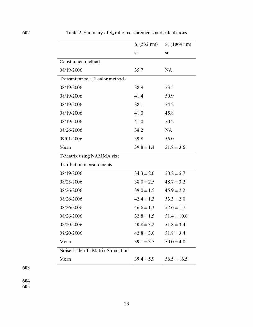
Table 2 summarizes the Sa ratios obtained for Saharan dust aerosols during NAMMA 596

using the three methods. The 532-nm values are fairly consistent while there is a 597

somewhat wider spread in the 1064-nm values. This is particularly interesting because 598

these measurements were made on various days and at various locations. 599

600

601

29

Table 2. Summary of Sa ratio measurements and calculations 602

Sa (532 nm)

sr

Sa (1064 nm)

sr

Constrained method

08/19/2006 35.7 NA

Transmittance + 2-color methods

08/19/2006 38.9 53.5

08/19/2006 41.4 50.9

08/19/2006 38.1 54.2

08/19/2006 41.0 45.8

08/19/2006 41.0 50.2

08/26/2006 38.2 NA

09/01/2006 39.8 56.0

Mean 39.8 ± 1.4 51.8 ± 3.6

T-Matrix using NAMMA size

distribution measurements

08/19/2006 34.3 ± 2.0 50.2 ± 5.7

08/25/2006 38.0 ± 2.5 48.7 ± 3.2

08/26/2006 39.0 ± 1.5 45.9 ± 2.2

08/26/2006 42.4 ± 1.3 53.3 ± 2.0

08/26/2006 46.6 ± 1.3 52.6 ± 1.7

08/26/2006 32.8 ± 1.5 51.4 ± 10.8

08/20/2006 40.8 ± 3.2 51.8 ± 3.4

08/20/2006 42.8 ± 3.0 51.8 ± 3.4

Mean 39.1 ± 3.5 50.0 ± 4.0

Noise Laden T- Matrix Simulation

Mean 39.4 ± 5.9 56.5 ± 16.5

603

604 605

30

6. Uncertainty Analysis of the modeled Sa ratios 606

In this section we attempt to propagate the uncertainty in the input variables to the 607

calculated Sa ratio and determine the overall uncertainty in the calculated dust 532-nm 608

and 1064-nm Sa ratios using a generalized analytical uncertainty equation. The 609

uncertainty equation is given by the Taylor series of the deviations (y –yo) of the output 610

(y) from its nominal value (yo) and is expressed in terms of the deviations of the i inputs 611

(x - xio ) from their nominal values. As in Morgan and Henrion [1990], for the first three 612

terms, the uncertainty is, 613

614

o

o

No o

i iii 1 X

N N 2o o

i i j ji ji 1 j 1 X

yy y (x x ) I

x

1 y (x x )(x x ) II

2 x x

1 (

3!

o

N N N 3o o o

i i j j k ki j ki 1 j 1 k 1 X

yx x )(x x )(x x ) ... III

x x x

(5) 615

616

The subscripts Xo denote derivatives evaluated at the nominal values. Assuming that 617

there are no covariances between the input variables, all the mixed derivatives in eq. (5) 618

would equal zero. The only terms that would not be zero are the first term and the terms 619

with i= j and i = j = k in summations II and III, i.e., second and third derivatives of the 620

variables, respectively. Since the covariances are not known we cannot make the 621

assumption that they are negligible. Given the uncertainties in the variables from which 622

the Sa ratio is calculated, the uncertainty in Sa can be estimated without making any 623

assumptions about covariances between inputs. To accomplish this we use Latin 624

31

Hypercube Sampling [LHS, Iman and Conover, 1980], a statistical sampling method in 625

which a distribution of plausible scenarios of parameter values is generated from a 626

multidimensional distribution. Unlike classical Monte Carlo sampling methods, LHS 627

precludes duplication by requiring that each square grid containing sample positions has 628

only one sample in each row and each column. For this study, we generate 500 variables 629

for each of the seven uncertain parameters used in the calculation of Sa. We then 630

randomly combine these variables to yield 500 instances or events. Each of these events 631

has a very high probability of yielding a unique Sa ratio. We then perform standard 632

descriptive statistics on the Sa values. 633

634

The mean and standard deviations of these values is an estimate of the nominal value and 635

uncertainty of dust Sa. We use the nominal (or central) values in Table 3, suggested by 636

the studies referenced in section 2, to generate the random scenarios. The fine mode radii, 637

coarse mode radii, and imaginary refractive indices are log normally distributed. The fine 638

and coarse geometric standard deviations (GSD), the real refractive indices, and the 639

aspect ratios are normally distributed. 640

641

The results obtained by using this method do not assume that the input variables are 642

independent of each other or that Sa ratio is linear in the individual input variables, i.e., 643

the second- and higher-order derivatives in Equation 5 are not necessarily equal to zero. 644

The statistics of the resulting Sa ratios provide an uncertainty envelop of the Sa ratio 645

estimates based on the uncertainty of the inputs. Moreover, the results can be used to 646

explore the sensitivity of the Sa ratios at each wavelength to the various aerosol 647

32

properties. In Figure 24, the 532-nm Sa ratios are well constrained with a standard 648

deviation of 15% of the mean after perturbing nominal input values shown in Table 3 and 649

similar to the distribution shown in Figure 22. The 1064-nm Sa ratios are much more 650

sensitive to the addition of noise as shown by the wide spread of 1064-nm Sa ratios in 651

Figure 24. A parameter that has a significant impact on the Sa ratios is the complex 652

refractive index. Figure 25 is a 2-D histogram of the 532- and 1064-nm Sa ratios as 653

functions of the real and imaginary parts of the refractive indices. The range of these 654

values is from 0.00067 to 0.006 for the imaginary part and 1.45 to 1.55 for the real part. 655

The 1064-nm Sa ratios are sensitive to changes in the refractive index throughout the 656

ranges of these variables. The 532-nm Sa ratio is sensitive to changes in the complex 657

refractive index at the lower ranges (Figures 25a and 25c). The highest density of 532-nm 658

Sa ratios are found in midranges of both the real and imaginary part, and these values are 659

insensitive to changes in the complex refractive index. Note that this variation is a total 660

derivative, i.e., all parameters are allowed to vary independently for the scenarios. The 661

1064-nm Sa ratios decrease with the complex index of refraction almost monotonically 662

through the range of values (Figures 25b and 25d) 663

664

665

33

Table 3. Ranges of the variables used to generate 500 random combinations of inputs for 666 T-Matrix calculations. The central values of the size distributions are based on the mean 667 values of the dust layer observed on 08/19/2006 during the NAMMA campaign 668 669

Parameter Minimum Maximum

Geometric Fine Radius 0.0216 0.194

Geometric Coarse Radius 0.188 1.69

Fine GSD 1.60 1.80

Coarse GSD 1.50 1.70

Real Refractive Index 1.45 1.55

Imaginary Refractive Index 0.00067 0.006

Aspect Ratio 1.70 2.30

670

7. Conclusion 671

We have determined the Sa ratios of Saharan dust layers using three methods: 672

transmittance constraint technique for lofted layers, in-situ extinction profile constraint 673

method, and T-Matrix calculations. We found quite robust Sa ratios at 532 nm and a 674

slightly wider spread at 1064 nm. The three methods yielded 532 nm and 1064 nm Sa 675

ratios that are quite close. Sa ratios of 39.8 ± 1.4 sr and 51.8 ± 3.6 sr at 532 nm and 1064 676

nm, respectively, were produced using the transmittance and 2-color methods applied to 677

CALIPSO measurements of Saharan dust lofted layers. T-Matrix calculations applied to 678

size distributions measured aboard the NASA DC-8 during NAMMA yielded Sa ratios of 679

39.1 ± 3.5 sr and 50.0 ± 4 sr at 532 nm and 1064 nm, respectively. The measured 680

extinction profile obtained by the aggregate of nephelometer measurements of total 681

34

scattering coefficient and the PSAP measurements of the absorption coefficient was used 682

to constrain the inversion of the CALIPSO measurements. This technique yielded a 532-683

nm Sa ratio of 35.7 sr for a dust layer and 25 sr for the aerosol in the marine boundary 684

layer. We perturbed seven microphysical and chemical properties of the dust aerosol and 685

computed the Sa ratios by randomly combining distributions of these parameters to assess 686

the uncertainty in the Sa calculation. This uncertainty simulation generated a mean (± 687

uncertainty) Sa of 39.4 (± 5.9) sr and 56.5 (± 16.5) sr at 532 nm and 1064 nm, 688

respectively, corresponding to percent uncertainties of 15% and 29%. The ratio of the Sa 689

ratios, Sa (1064 nm) /Sa (532 nm) = 1.3 ± 0.13, and nearly normally distributed. The 690

simulation revealed that Sa is insensitive to the middle range of refractive indices at 532 691

nm and nearly monotonically dependent on the refractive indices at 1064 nm. This 692

explains the observed robust Sa ratios at 532 nm and relatively wide spread of Sa at 1064 693

nm 694

This study examined a wide range of dust loadings in various locations within ~1250 km 695

of Saharan Desert source regions on different days. The Sa ratios do not change 696

significantly with dust loading, suggesting the dust microphysical and chemical 697

properties do not vary appreciably. The profile of Sa ratios at 532 nm are very close to 40 698

sr using different methods and on different days. There is a wider variation in the 1064 699

nm Sa ratios for all methods. It is possible that the variation of Sa at 1064 nm is driven by 700

a higher sensitivity to changes in the complex index of refraction at the 1064 nm 701

wavelength. The ratio of Sa ratios at the two wavelengths [Sa (1064 nm)/Sa (532 nm)] is 702

1.3 ± 0.13. 703

35

8. Acknowledgements 704

We gratefully acknowledge funding support from the NASA Radiation Sciences and 705

Atmospheric Composition Programs, respectively managed by Drs. Hal Maring and 706

Bruce Doddridge, and the CALIPSO team for the satellite data and many discussions 707

708

36

9. References 709

Ackermann, J. (1998), The extinction-to-backscatter ratio of tropospheric aerosol: A 710 numerical study, J. Atmos. Ocean Tech., 15, 1043-1050. 711 712 Anderson, T. L., and J. A. Ogren (1998), Determining aerosol radiative properties using 713 the TSI 3563 integrating nephelometer, Aerosol Sci. Technol., 29(1), 57-69. 714 715 Anderson, T. L., S. J. Masonis, D. S. Covert, and R. J. Charlson (2000), In situ 716 measurements of the aerosol extinction-to-backscatter ratio at a polluted continental site, 717 J. Geophys. Res., 105(D22), 26907-26915. 718 719 Ansmann, A., H. Baars, M. Tesche, D. Muller, D. Althausen, R. Engelmann, T. 720 Pauliquevis, and P. Artaxo (2009), Dust and smoke transport from Africa to South 721 America: Lidar profiling over Cape Verde and the Amazon rainforest, Geophysical 722 Research Letters, 36, 5. 723 724 Barnaba, F., and G. P. Gobbi (2004), Modeling the aerosol extinction versus backscatter 725 relationship for lidar applications: Maritime and continental conditions, J. Atmos. Ocean 726 Tech., 21(3), 428-442. 727 728 Berthier, S., P. Chazette, P. Couvert, J. Pelon, F. Dulac, F. Thieuleux, C. Moulin, and T. 729 Pain (2006), Desert dust aerosol columnar properties over ocean and continental Africa 730 from Lidar in-Space Technology Experiment (LITE) and Meteosat synergy, J. Geophys. 731 Res.-Atmos., 111(D21), 20. 732 733 Cattrall, C., J. Reagan, K. Thome, and O. Dubovik (2005), Variability of aerosol and 734 spectral lidar and backscatter and extinction ratios of key aerosol types derived from 735 selected Aerosol Robotic Network locations, J. Geophys. Res., 110(D10). 736 737 Chen, G., L. D. Ziemba, D. A. Chu, K. L. Thornhill, G. L. Schuster, E. L. Winstead, G. S. 738 Diskin, R. A. Ferrare, S. P. Burton, S. Ismail, S. A. Kooi, A. H. Omar, D. L. Slusher, M. 739 M. Kleb, C. H. Twohy, and B. E. Anderson (2010), Observations of Saharan Dust 740 Microphysical and Optical Properties from the Eastern Atlantic during NAMMA 741 Airborne Field Campaign, Atmos. Chem. Phys., (submitted). 742 743 d'Almeida, G. A., P. Koepke, and E. P. Shettle (1991), Atmospheric Aerosols: Global 744 Climatology and Radiative Characteristics, A. Deepak Publishing, Hampton, VA. 745 746 DeMott, P. J., K. Sassen, M. R. Poellot, D. Baumgardner, D. C. Rogers, S. D. Brooks, A. 747 J. Prenni, and S. M. Kreidenweis (2003), African dust aerosols as atmospheric ice nuclei, 748 Geophysical Research Letters, 30(14). 749 750

37

Di Iorio, T., A. di Sarra, W. Junkermann, M. Cacciani, G. Fiocco, and D. Fua (2003), 751 Tropospheric aerosols in the Mediterranean: 1. Microphysical and optical properties, J. 752 Geophys. Res., 108(D10). 753 754 Di Iorio, T., A. di Sarra, D. M. Sferlazzo, M. Cacciani, D. Meloni, F. Monteleone, D. 755 Fua, and G. Fiocco (2009), Seasonal evolution of the tropospheric aerosol vertical profile 756 in the central Mediterranean and role of desert dust, J. Geophys. Res.-Atmos., 114, 9. 757 758 Dubovik, O., B. N. Holben, T. F. Eck, A. Smirnov, Y. J. Kaufman, M. D. King, D. Tanre, 759 and I. Slutsker (2002), Variability of absorption and optical properties of key aerosol 760 types observed in worldwide locations, J. Atmos. Sci., 59, 590-608. 761 762 Dunion, J. P., and C. S. Velden (2004), The impact of the Saharan air layer on Atlantic 763 tropical cyclone activity, Bulletin of the American Meteorological Society, 85(3), 353-+. 764 765 Eidhammer, T., D. C. Montague, and T. Deshler (2008), Determination of index of 766 refraction and size of supermicrometer particles from light scattering measurements at 767 two angles, J. Geophys. Res.-Atmos., 113(D16), 19. 768 769 Formenti, P., W. Elbert, W. Maenhaut, J. Haywood, and M. O. Andreae (2003), 770 Chemical composition of mineral dust aerosol during the Saharan Dust Experiment 771 (SHADE) airborne campaign in the Cape Verde region, September 2000, J. Geophys. 772 Res.-Atmos., 108(D18). 773 774 Graham, B., P. Guyon, W. Maenhaut, P. E. Taylor, M. Ebert, S. Matthias-Maser, O. L. 775 Mayol-Bracero, R. H. M. Godoi, P. Artaxo, F. X. Meixner, M. A. L. Moura, C. Rocha, R. 776 Van Grieken, M. M. Glovsky, R. C. Flagan, and M. O. Andreae (2003), Composition and 777 diurnal variability of the natural Amazonian aerosol, J. Geophys. Res.-Atmos., 108(D24). 778 779 Heintzenberg, J. (2009), The SAMUM-1 experiment over Southern Morocco: overview 780 and introduction, Tellus Ser. B-Chem. Phys. Meteorol., 61(1), 2-11. 781 782 Hill, S. C., A. C. Hill, and P. W. Barber (1984), Light-scattering by size shape 783 distributions of soil particles and spheroids, Applied Optics, 23(7), 1025-1031. 784 785 Hu, Y., D. Winker, M. Vaughan, B. Lin, A. Omar, C. Trepte, D. Flittner, P. Yang, S. L. 786 Nasiri, B. Baum, W. Sun, Z. Liu, Z. Wang, S. Young, K. Stamnes, J. Huang, R. Kuehn, 787 and R. Holz (2009), CALIPSO/CALIOP Cloud Phase Discrimination Algorithm, J. 788 Atmos. Oceanic Technol., 26, 2293-2309. 789 790 Iman, R. L., and W. J. Conover (1980), Small sample sensitivity analysis techniques for 791 computer-models, with an application to risk assessment, Communications in Statistics 792 Part a-Theory and Methods, 9(17), 1749-1842. 793 794 Ismail, S., R. A. Ferrare, E. V. Browell, S. A. Kooi, J. P. Dunion, G. Heymsfield, A. Notari, C. 795 F. Butler, S. Burton, M. Fenn, T. N. Krishnamurti, M. K. Biswas, G. Chen, and B. Anderson 796

38

(2010), LASE measurements of water vapor, aerosol, and cloud distributions in Saharan 797 air layers and Tropical disturbances 798 J. Atmos. Sci., In Press. 799 800 Israelevich, P. L., E. Ganor, Z. Levin, and J. H. Joseph (2003), Annual variations of 801 physical properties of desert dust over Israel, J. Geophys. Res., 108. 802 803 Kalashnikova, O. V., and I. N. Sokolik (2002), Importance of shapes and compositions of 804 wind-blown dust particles for remote sensing at solar wavelengths, Geophys. Res. Letts., 805 29(10), 38 31-34. 806 807 Kalashnikova, O. V., and I. N. Sokolik (2004), Modeling the radiative properties of 808 nonspherical soil-derived mineral aerosols, J. Quant. Spectroscopy & Radiative Transfer, 809 87(2), 137-166. 810 811 Kandler, K., L. Schutz, C. Deutscher, M. Ebert, H. Hofmann, S. Jackel, R. Jaenicke, P. 812 Knippertz, K. Lieke, A. Massling, A. Petzold, A. Schladitz, B. Weinzierl, A. 813 Wiedensohler, S. Zorn, and S. Weinbruch (2009), Size distribution, mass concentration, 814 chemical and mineralogical composition and derived optical parameters of the boundary 815 layer aerosol at Tinfou, Morocco, during SAMUM 2006, Tellus Ser. B-Chem. Phys. 816 Meteorol., 61(1), 32-50. 817 818 Kaufman, Y. J., I. Koren, L. A. Remer, D. Tanre, P. Ginoux, and S. Fan (2005), Dust 819 transport and deposition observed from the Terra-Moderate Resolution Imaging 820 Spectroradiometer ( MODIS) spacecraft over the Atlantic ocean, J. Geophys. Res.-821 Atmos., 110(D10). 822 823 Liu, Z., A. Omar, M. Vaughan, J. Hair, C. Kittaka, Y. X. Hu, K. Powell, C. Trepte, D. 824 Winker, C. Hostetler, R. Ferrare, and R. Pierce (2008), CALIPSO lidar observations of 825 the optical properties of Saharan dust: A case study of long-range transport, J. Geophys. 826 Res., 113(D7). 827 828 Liu, Z. Y., M. Vaughan, D. Winker, C. Kittaka, B. Getzewich, R. Kuehn, A. Omar, K. 829 Powell, C. Trepte, and C. Hostetler (2009), The CALIPSO Lidar Cloud and Aerosol 830 Discrimination: Version 2 Algorithm and Initial Assessment of Performance, J. Atmos. 831 Oceanic Technol., 26(7), 1198-1213. 832 833 Maring, H., D. L. Savoie, M. A. Izaguirre, L. Custals, and J. S. Reid (2003), Mineral dust 834 aerosol size distribution change during atmospheric transport, J. Geophys. Res., 835 108(D19). 836 837 Mie, G. (1908), Beigrade zur optik trüber medien, speziell kolloidaler metallösungen, 838 Ann. Physik, 25(4), 337-445. 839 840

39

Mischenko, M. I., A. A. Lacis, B. E. Carlson, and L. D. Travis (1995), Nonsphericity of 841 dust-like tropospheric aerosols: implications for aerosol remote sensing and climate 842 modeling, Geophys. Res. Letts., 22(9), 1077-1080. 843 844 Mishchenko, M. I. (1991), Light-scattering by randomly oriented axially symmetrical 845 particles, J. Opt. Soc. Am. A, 8(6), 871-882. 846 847 Mishchenko, M. I. (1993), Light-scattering by size shape distributions of randomly 848 oriented axially-symmetrical particles of a size comparable to a wavelength, Applied 849 Optics, 32(24), 4652-4666. 850 851 Mishchenko, M. I., and L. D. Travis (1994), T-matrix computations of light-scattering by 852 large spheroidal particle, Optics Comm., 109(1-2), 16-21. 853 854 Mishchenko, M. I., L. D. Travis, and A. Macke (1996a), Scattering of light by 855 polydisperse, randomly oriented, finite circular cylinders, Applied Optics, 35(24), 4927-856 4940. 857 858 Mishchenko, M. I., L. D. Travis, and D. W. Mackowski (1996b), T-matrix computations 859 of light scattering by nonspherical particles: A review, J. Quant. Spectros. Rad. Trans., 860 55(5), 535-575. 861 862 Mishchenko, M. I., and L. D. Travis (1998), Capabilities and limitations of a current 863 FORTRAN implementation of the T-matrix method for randomly oriented, rotationally 864 symmetric scatterers. 865 866 Morgan, M. G., and M. Henrion (1990), Uncertainty: A Guide to dealing with 867 uncertainty in quantitative risk and policy analysis, 2 ed., 332 pp., Cambridge University 868 Press, Cambridge. 869 870 Muller, D., A. Ansmann, I. Mattis, M. Tesche, U. Wandinger, D. Althausen, and G. 871 Pisani (2007), Aerosol-type-dependent lidar ratios observed with Raman lidar, J. 872 Geophys. Res., 112(D16). 873 874 Müller, D., F. Wagner, D. Althausen, U. Wandinger, and A. Ansmann (2000), Physical 875 properties of the Indian aerosol plume derived from six-wavelength lidar observations on 876 25 March 1999 of the Indian Ocean Experiment, Geophys. Res. Letts., 27(9), 1403-1406. 877 878 Murayama, T., S. J. Masonis, J. Redemann, T. L. Anderson, B. Schmid, J. M. Livingston, 879 P. B. Russell, B. Huebert, S. G. Howell, C. S. McNaughton, A. Clarke, M. Abo, A. 880 Shimizu, N. Sugimoto, M. Yabuki, H. Kuze, S. Fukagawa, K. Maxwell-Meier, R. J. 881 Weber, D. A. Orsini, B. Blomquist, A. Bandy, and D. Thornton (2003), An 882 intercomparison of lidar-derived aerosol optical properties with airborne measurements 883 near Tokyo during ACE-Asia, J. Geophys. Res., 108(D23). 884 885

40

Nakajima, T., M. Tanaka, M. Yamano, M. Shiobara, K. Arao, and Y. Nakanishi (1989), 886 Aerosol optical characteristics in the yellow sand events observed in may, 1982 at 887 Nagasaki .2. Models, J. Meteor. Soc. Japan, 67(2), 279-291. 888 889 Okada, K., A. Kobayashi, Y. Iwasaka, H. Naruse, T. Tanaka, and O. Nemoto (1987), 890 Features of individual asian dust-storm particles collected at Nagoya, Japan, J. Meteor. 891 Soc. Japan, 65(3), 515-521. 892 893 Okin, G. S., N. Mahowald, O. A. Chadwick, and P. Artaxo (2004), Impact of desert dust 894 on the biogeochemistry of phosphorus in terrestrial ecosystems, Global Biogeochemical 895 Cycles, 18(2). 896 897 Omar, A., D. Winker, C. Kittaka, M. Vaughan, Z. Liu, Y. Hu, C. Trepte, R. Rogers, R. 898 Ferrare, K. P. Lee, R. Kuehn, and C. Hostetler (2009), The CALIPSO automated aerosol 899 classification and lidar ratio selection algorithm, J. Atmos. Oceanic Technol., 26(10), 900 1994-2014. 901 902 Omar, A. H., S. Biegalski, S. M. Larson, and S. Landsberger (1999), Particulate 903 contributions to light extinction and local forcing at a rural Illinois site, Atmospheric 904 Environment, 33(17), 2637-2646. 905 906 Perry, R. J., A. J. Hunt, and D. R. Huffman (1978), Experimental determinations of 907 Mueller scattering matrices for nonspherical particles 908 Applied Optics, 17(17), 2700-2710. 909 910 Petzold, A., K. Rasp, B. Weinzierl, M. Esselborn, T. Hamburger, A. Dornbrack, K. 911 Kandler, L. Schutz, P. Knippertz, M. Fiebig, and A. Virkkula (2009), Saharan dust 912 absorption and refractive index from aircraft-based observations during SAMUM 2006, 913 Tellus Ser. B-Chem. Phys. Meteorol., 61(1), 118-130. 914 915 Platt, C. M. R. (1973), Lidar and Radiometric Observations of Cirrus Clouds, J. Atmos. 916 Sci., 30, 1191-1204. 917 918 Prospero, J. M., and T. N. Carlson (1971), Saharan dust in atmosphere of northern 919 equatorial Atlantic ocean - a major constituent of marine aerosol 920 Bulletin of the American Meteorological Society, 52(11), 1138-&. 921 922 Prospero, J. M., and T. N. Carlson (1972), Vertical and areal distribution of Saharan dust 923 over western equatorial North-Atlantic Ocean 924 J. Geophys. Res., 77(27), 5255-5265. 925 926 Rodhe, H. (2009), Special issue: Results of the Saharan Mineral Dust Experiment 927 (SAMUM-1) 2006 Preface, Tellus Ser. B-Chem. Phys. Meteorol., 61(1), 1-1. 928 929

41

Sasano, Y., and E. V. Browell (1989), Light scattering characteristics of various aerosol 930 types derived from multiple wavelength lidar observations, Applied Optics, 28, 1670-931 1679. 932 933 Savoie, D., and J. M. Prospero (1976), Saharan aerosol transport across Atlantic ocean - 934 characteristics of input and output, Bull Am. Meteorol. Soc., 57(1), 145-145. 935 936 Schladitz, A., T. Muller, N. Kaaden, A. Massling, K. Kandler, M. Ebert, S. Weinbruch, 937 C. Deutscher, and A. Wiedensohler (2009), In situ measurements of optical properties at 938 Tinfou (Morocco) during the Saharan Mineral Dust Experiment SAMUM 2006, Tellus 939 Ser. B-Chem. Phys. Meteorol., 61(1), 64-78. 940 941 Sokolik, I. N., and O. B. Toon (1996), Direct radiative forcing by anthropogenic airborne 942 mineral aerosols, Nature, 381(6584), 681-683. 943 944 Tesche, M., A. Ansmann, D. Muller, D. Althausen, I. Mattis, B. Heese, V. Freudenthaler, 945 M. Wiegner, M. Esselborn, G. Pisani, and P. Knippertz (2009), Vertical profiling of 946 Saharan dust with Raman lidars and airborne HSRL in southern Morocco during 947 SAMUM, Tellus B, 61(1), 144-164. 948 949 Vaughan, M. A., Z. Liu, and A. H. Omar (2004), Multi-wavelength analysis of a lofted 950 aerosol layer measured by LITE, paper presented at 22nd International Laser Radar 951 Conference, European Space Agency, Matera, Italy, 12-16 July, 2004. 952 953 Vaughan, M. A., K. A. Powell, R. E. Kuehn, S. A. Young, D. M. Winker, C. A. 954 Hostetler, W. H. Hunt, Z. Y. Liu, M. J. McGill, and B. J. Getzewich (2009), Fully 955 Automated Detection of Cloud and Aerosol Layers in the CALIPSO Lidar 956 Measurements, J. Atmos. Oceanic Technol., 26(10), 2034-2050. 957 958 Virkkula, A., N. C. Ahlquist, D. S. Covert, W. P. Arnott, P. J. Sheridan, P. K. Quinn, and 959 D. J. Coffman (2005), Modification, calibration and a field test of an instrument for 960 measuring light absorption by particles, Aerosol Sci. Technol., 39(1), 68-83. 961 962 Volz, F. E. (1973), Infrared Optical Constants of Ammonium Sulfate, Sahara Dust, 963 Volcanic Pumice, and Flyash, Appl. Opt., 12(3), 564-568. 964 965 Voss, K. J., E. J. Welton, P. K. Quinn, J. Johnson, A. M. Thompson, and H. R. Gordon 966 (2001), Lidar measurements during Aerosols99, J. Geophys. Res., 106(D18), 20821-967 20831. 968 969 Waterman, P. C. (1971), Symmetry, unitarity, and geometry in electromagnetic 970 scattering, Physical Review D, 3(4), 825-&. 971 972 Winker, D., M. Vaughan, A. Omar, Y. Hu, K. Powell, Z. Liu, W. Hunt, and S. A. Young 973 (2009), Overview of the CALIPSO mission and CALIOP data processing algorithms J. 974 Atmos. Ocean. Tech., 26, 2310-2323. 975

42

976 Winker, D. M., W. H. Hunt, and M. J. McGill (2007), Initial performance assessment of 977 CALIOP, Geophys. Res. Letts., 34(19). 978 979 Wong, S., and A. E. Dessler (2005), Suppression of deep convection over the tropical 980 North Atlantic by the Saharan Air Layer, Geophysical Research Letters, 32(9). 981 982 Young, S. A. (1995), Analysis of lidar backscatter profiles in optically thin clouds, 983 Applied Optics, 34(30), 7019-7031. 984 985 986 Figure 1. (a) A Two-dimensional probability plot of NAMMA in situ size distributions 987 measured in a dust layer over a 22 minute period (~260 size distributions) during Flight 4 988 on August 19, 2006. The mean measured size distribution is denoted by the yellow line, 989 and (b) the best approximate bimodal log-normal particle size distribution (blue squares) 990 with fine (coarse) mean radius of 0.0648 (0.5627) μm and a fine (coarse) geometric 991 standard deviation of 1.696 (1.572) fitted to the average measured size distribution (red 992 squares). 993

994

43

995

0.04 0.045 0.05 0.055 0.06 0.065 0.070

0.02

0.04

0.06

0.08

0.1

0.12

Geometric Mean Radius

Frac

tion

al F

requ

ency

0.25 0.3 0.35 0.4 0.45 0.5 0.55 0.6 0.650

0.02

0.04

0.06

0.08

0.1

0.12

0.14

Geometric Mean Radius

Frac

tion

al F

requ

ency

(μm) (μm)

(b)(a)

1.25 1.3 1.35 1.4 1.45 1.5 1.55 1.6 1.65 1.7 1.750

0.01

0.02

0.03

0.04

0.05

0.06

Geometric Standard Deviation

Frac

tion

al F

requ

ency

1 1.1 1.2 1.3 1.4 1.5 1.6 1.7 1.80

0.02

0.04

0.06

0.08

0.1

0.12

Geometric Standard Deviation

Frac

tion

al F

requ

ency

(d)(c)

0.04 0.045 0.05 0.055 0.06 0.065 0.070

0.02

0.04

0.06

0.08

0.1

0.12

Geometric Mean Radius

Frac

tion

al F

requ

ency

0.25 0.3 0.35 0.4 0.45 0.5 0.55 0.6 0.650

0.02

0.04

0.06

0.08

0.1

0.12

0.14

Geometric Mean Radius

Frac

tion

al F

requ

ency

(μm) (μm)

(b)(a)

1.25 1.3 1.35 1.4 1.45 1.5 1.55 1.6 1.65 1.7 1.750

0.01

0.02

0.03

0.04

0.05

0.06

Geometric Standard Deviation

Frac

tion

al F

requ

ency

1 1.1 1.2 1.3 1.4 1.5 1.6 1.7 1.80

0.02

0.04

0.06

0.08

0.1

0.12

Geometric Standard Deviation

Frac

tion

al F

requ

ency

(d)(c)

996

Figure 2. The distributions of the fine (a) and coarse (b) geometric mean radii and the 997 fine (c) and coarse (d) geometric standard deviations for a dense elevated dust layer 998 measured during a flight on August 25, 2006. 999

1000

44

1001

0.1

1

10

100

0 30 60 90 120 150 180

Coarse Particles Phase Function Fine Particles Phase FunctionPhase Function

Phas

e Fu

ncti

on (5

32 n

m)

Scattering Angle (deg)

(a)

0.1

1

10

100

0 30 60 90 120 150 180

Coarse Particles Phase Function Fine Particles Phase FunctionPhase Function

Phas

e Fu

ncti

on (1

064

nm)

Scattering Angle (deg)

(b)

1002

Figure 3. The (a) 532-nm and (b) 1064 nm Saharan dust phase functions calculated from 1003 the size distributions measured aboard NASA DC-8 during Flight 4 on August 19, 2006. 1004

1005

45

1006

0

2

4

6

8

10

12

49,390 53,880 58,370 62,860 67,350

Alti

tude

(km

)

Seconds after 00:00 UT

In Situ Profile Flight Path

ab

c

d

e

1007

Figure 4. The DC-8 altitudinal flight path showing the segment during which the in situ 1008 measurements were made. The direct CALIPSO underflights are the five segments (a, b, 1009 c, d, and e) at the highest altitudes. The time is in seconds after midnight UTC. 1010

1011

46

1012

0.0 0.1 0.2 0.3 0.4 0.5Aerosol Optical Depth

MODIS 04 V.5 OPTICAL DEPTH

DC-8C

AL

IPS

O

(a)

MODIS 04 V.5 OPTICAL DEPTH

DC-8C

AL

IPS

O

MODIS 04 V.5 OPTICAL DEPTH

DC-8

MODIS 04 V.5 OPTICAL DEPTH

DC-8DC-8C

AL

IPS

O

(a)

MOPPITT CO

CA

LIP

SO

(b)

MOPPITT CO

CA

LIP

SO

MOPPITT CO

CA

LIP

SO

(b)

0.0 0.5 1.0 1.5 2.0 2.5 3.0x1018 [molec/cm2] 1013

Figure 5. CALIPSO flight tracks superimposed on (a) the MODIS optical depth and (b) 1014 the MOPPITT CO concentrations. The DC-8 flight track for August 19, 2006 is shown 1015 by the black lines in the middle of both figures. The blue dots in (a) denote the portion of 1016 the DC-8 flight segment during which the in-situ measurements were taken. Daytime 1017 CALIPSO tracks run from the southeast to the northwest while the nighttime tracks run 1018 from northeast to the southwest. 1019

1020

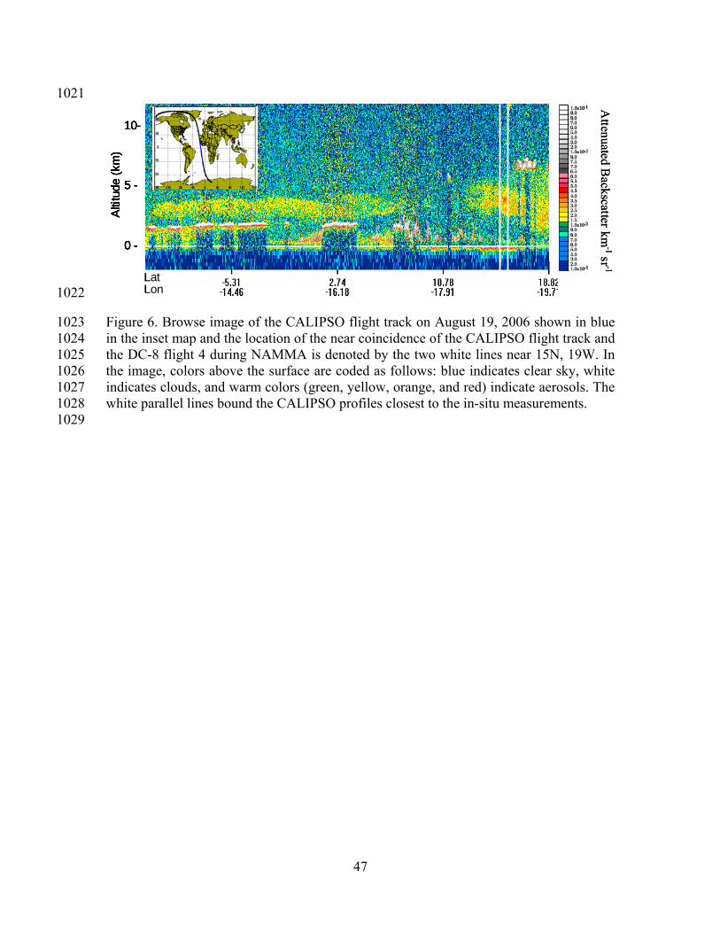
47

1021

10-

5 -

0 -

Alti

tude

(km

)

LatLon

10-

5 -

0 -

Alti

tude

(km

)

LatLon

Attenuated B

ackscatter km-1

sr -1

10-

5 -

0 -

Alti

tude

(km

)

LatLon

10-

5 -

0 -

Alti

tude

(km

)

LatLon

Attenuated B

ackscatter km-1

sr -1

1022

Figure 6. Browse image of the CALIPSO flight track on August 19, 2006 shown in blue 1023 in the inset map and the location of the near coincidence of the CALIPSO flight track and 1024 the DC-8 flight 4 during NAMMA is denoted by the two white lines near 15N, 19W. In 1025 the image, colors above the surface are coded as follows: blue indicates clear sky, white 1026 indicates clouds, and warm colors (green, yellow, orange, and red) indicate aerosols. The 1027 white parallel lines bound the CALIPSO profiles closest to the in-situ measurements. 1028

1029

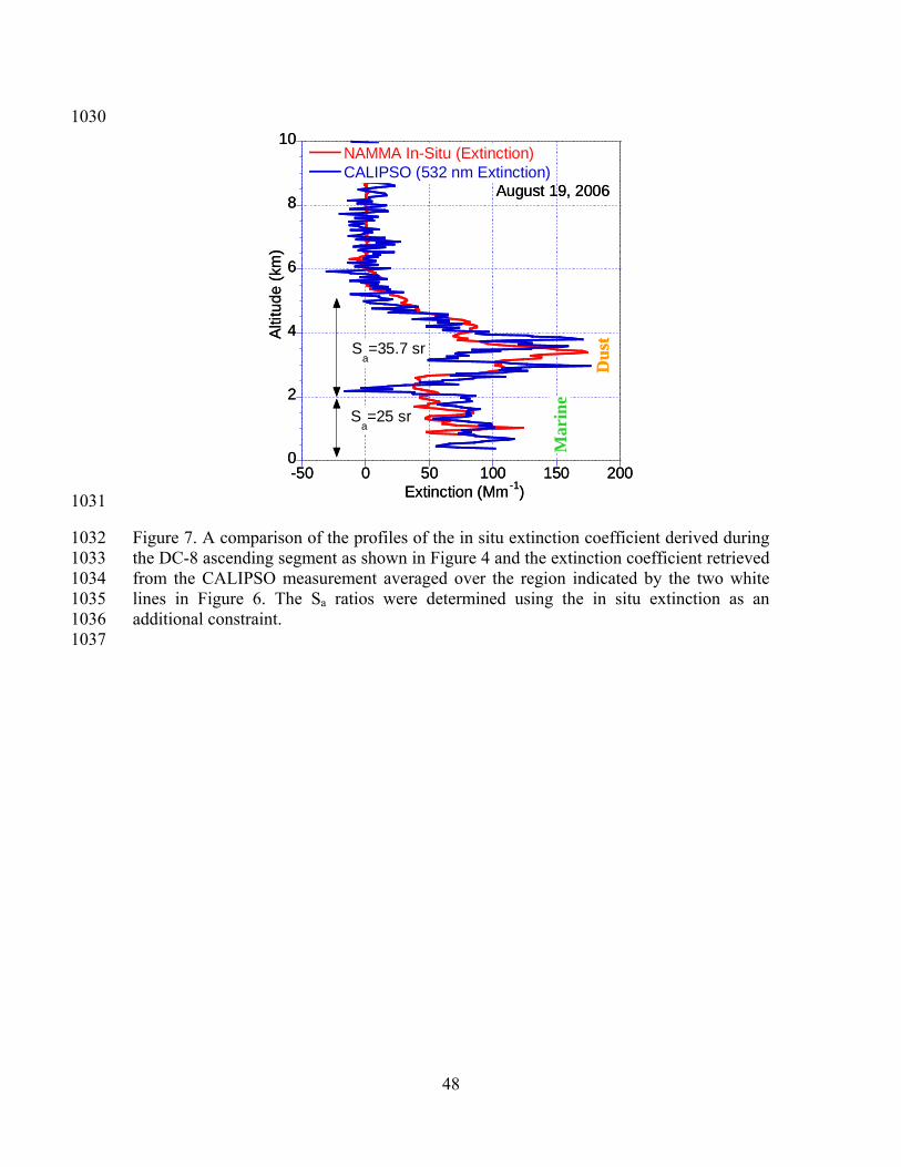
48

1030

0

2

4

6

8

10

-50 0 50 100 150 200

NAMMA In-Situ (Extinction)CALIPSO (532 nm Extinction)

Alti

tud

e (

km)

Extinction (Mm-1)

August 19, 2006

Sa=35.7 sr

Sa=25 sr

Du

st

Mar

ine

0

2

4

6

8

10

-50 0 50 100 150 200

NAMMA In-Situ (Extinction)CALIPSO (532 nm Extinction)

Alti

tud

e (

km)

Extinction (Mm-1)

August 19, 2006

Sa=35.7 sr

Sa=25 sr

Du

st

Mar

ine

1031

Figure 7. A comparison of the profiles of the in situ extinction coefficient derived during 1032 the DC-8 ascending segment as shown in Figure 4 and the extinction coefficient retrieved 1033 from the CALIPSO measurement averaged over the region indicated by the two white 1034 lines in Figure 6. The Sa ratios were determined using the in situ extinction as an 1035 additional constraint. 1036 1037

49

1038

Figure 8. Aerosol scattering ratio (a/m at 815 nm) image measured by the Lidar 1039 Atmospheric Sensing Experiment (LASE) aboard DC-8 during the ascending segment 1040 passing through a Sahara Air Layer (SAL) and the underflight of CALIPSO as shown in 1041 Figure 4. The DC-8 point of nearest approach to the CALIPSO flight track is near 15oN-1042 19oW. 1043 1044

50

 

0.0

2.0

4.0

6.0

8.0

10.0

-8.8 -6.2 -3.7 -1.1 1.5 4.0 6.6 9.2 11.7 14.3 16.8-13.7 -17.0-16.5-15.9-15.4-14.8-14.3 -17.6 -18.1 -18.7 -19.3

LatLon

0.0

2.0

4.0

6.0

8.0

10.0

Alt

itud

e (k

m)

Alt

itud

e (k

m)

(a) Cloud Aerosol DiscriminationCloud

Aerosol

Marine Dust PollutedContinental Clean

Continental

Polluted Dust

Smoke

(b) Aerosol Classification

0.0

2.0

4.0

6.0

8.0

10.0

-8.8 -6.2 -3.7 -1.1 1.5 4.0 6.6 9.2 11.7 14.3 16.8-13.7 -17.0-16.5-15.9-15.4-14.8-14.3 -17.6 -18.1 -18.7 -19.3

LatLon

0.0

2.0

4.0

6.0

8.0

10.0

Alt

itud

e (k

m)

Alt

itud

e (k

m)

0.0

2.0

4.0

6.0

8.0

10.0

0.0

2.0

4.0

6.0

8.0

10.0

-8.8 -6.2 -3.7 -1.1 1.5 4.0 6.6 9.2 11.7 14.3 16.8-13.7 -17.0-16.5-15.9-15.4-14.8-14.3 -17.6 -18.1 -18.7 -19.3

LatLon

-8.8 -6.2 -3.7 -1.1 1.5 4.0 6.6 9.2 11.7 14.3 16.8-13.7 -17.0-16.5-15.9-15.4-14.8-14.3 -17.6 -18.1 -18.7 -19.3

LatLon

0.0

2.0

4.0

6.0

8.0

10.0

0.0

2.0

4.0

6.0

8.0

10.0

Alt

itud

e (k

m)

Alt

itud

e (k

m)

(a) Cloud Aerosol DiscriminationCloud

Aerosol

Marine Dust PollutedContinental Clean

Continental

Polluted Dust

SmokeMarine Dust PollutedContinental Clean

Continental

Polluted Dust

Smoke

(b) Aerosol Classification

1045

Figure 9. Products of the CALIPSO (a) cloud-aerosol discrimination and (b) aerosol 1046 classification schemes for the data in the browse image shown in Figure 6. The cloud 1047 aerosol discrimination shows the extensive aerosol layer at 3 km and the aerosol 1048 classification image shows that this aerosol is a Saharan dust layer to the north and a 1049 polluted dust and smoke layer to the south. 1050 1051

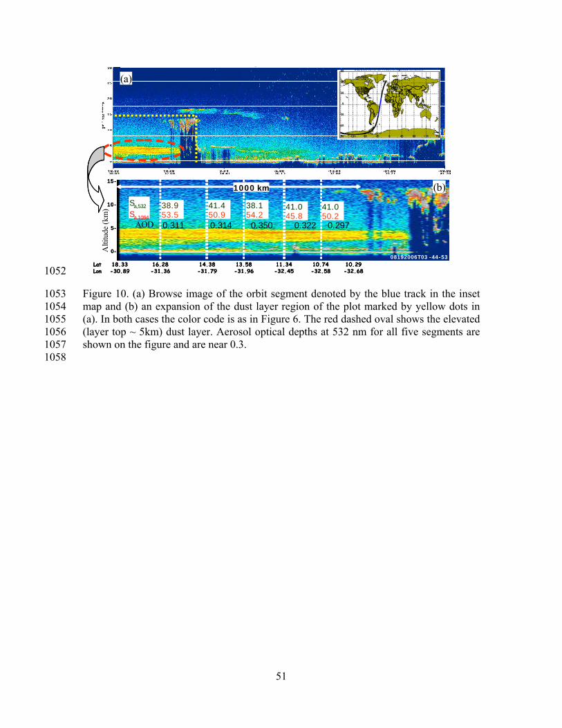
51

1000 km

08192006T03 -44-53

15-

10-

5-

0-

38.953.5

41.450.9

38.154.2

41.045.8

41.050.2

Sa,532

Sa,1064

08192006T03 -44-53

15-

10-

5-

0-

18.33-30.89

10.29-32.68

13.58-31.96

16.28-31.36

14.38-31.79

10.74-32.58

11.34-32.45

LatLon

18.33-30.89

10.29-32.68

13.58-31.96

16.28-31.36

14.38-31.79

10.74-32.58

11.34-32.45

LatLon

38.953.5

41.450.9

38.154.2

41.045.8

41.050.2

Sa,532

Sa,1064

0.311 0.322 0.2970.3500.314

1000 km

Alti

tude

(km

)

AOD

(a)

(b)

1052

Figure 10. (a) Browse image of the orbit segment denoted by the blue track in the inset 1053 map and (b) an expansion of the dust layer region of the plot marked by yellow dots in 1054 (a). In both cases the color code is as in Figure 6. The red dashed oval shows the elevated 1055 (layer top ~ 5km) dust layer. Aerosol optical depths at 532 nm for all five segments are 1056 shown on the figure and are near 0.3. 1057

1058

52

1059

MODIS 04 V.5 OPTICAL DEPTH

(a)

0.0 0.1 0.2 0.3 0.4 0.5Aerosol Optical Depth

MOPPITT CO(b)

0.0 0.5 1.0 1.5 2.0 2.5 3.0x1018 [molec/cm2] 1060

Figure 11. CALIPSO flight tracks superimposed on the (a) MODIS optical depth and the 1061 (b) MOPPITT CO concentrations. The CALIPSO flight tracks are colored cyan and grey 1062 in the MODIS and MOPPITT images, respectively. The DC-8 flight track for August 26, 1063 2006 is shown by the heart shaped drawing in the middle of both figures. The CALIPSO 1064 underflight segment is the portion of the flight track in alignment with the CALIPSO 1065 flight track in cyan or grey in (a) or (b), respectively. The DC-8 in situ data for this 1066 obtained during the descent flight segment shown by a red dashed tilted oval in (a). 1067

1068

53

1069

Alt

itu

de

(km

)

LatLon 1070

Figure 12. Browse image of the CALIPSO flight track shown in green in the inset map 1071 and the location of the near coincidence (in space) of the CALIPSO flight track and the 1072 DC-8 flight 8 on August 26, 2006. The color code is as in Fig. 6. The white lines denote 1073 the CALIPSO data used for comparison with the DC-8 measurements. 1074

1075

54

1076

0

2

4

6

8

10

-40 0 40 80 120 160 200

NAMMA In-Situ (Extinction)CALIPSO Extinction (532 nm)

Alti

tud

e (

km)

Extinction(Mm-1)

08262006 Ascent Leg

(a)

1077

Figure 13. A comparison of the NAMMA in situ extinction profile and the extinction 1078 profile calculated from CALIPSO’s attenuated backscatter measurement using 532 nm Sa 1079 ratio of 38.2 sr obtained using the transmittance method. The two measurements both 1080 taken on August 26, 2006 are offset by 2 hours and ~1250 km. 1081

1082

55

1083

(a) MODIS 04 V.5 AOD

(a)(a)(a)(a)(a)(a)

0.0 0.1 0.2 0.3 0.4 0.5Aerosol Optical Depth

September 1, 2006 (b)September 1, 2006 (b)September 1, 2006September 1, 2006September 1, 2006 (b)September 1, 2006 (b)September 1, 2006September 1, 2006September 1, 2006 (b)September 1, 2006September 1, 2006September 1, 2006 (b)September 1, 2006September 1, 2006September 1, 2006September 1, 2006

(b) MOPPITT CO

DC-8

0.0 0.5 1.0 1.5 2.0 2.5 3.0x1018 [molec/cm2] 1084

Figure 14. CALIPSO flight tracks superimposed on the (a) MODIS optical depth and the 1085 (b) MOPPITT CO concentrations. The CALIPSO flight tracks are colored cyan and grey 1086 in the MODIS and MOPPITT images. The DC-8 flight track for September 1, 2006 is 1087 shown by the black lines in the middle of both figures. 1088

1089

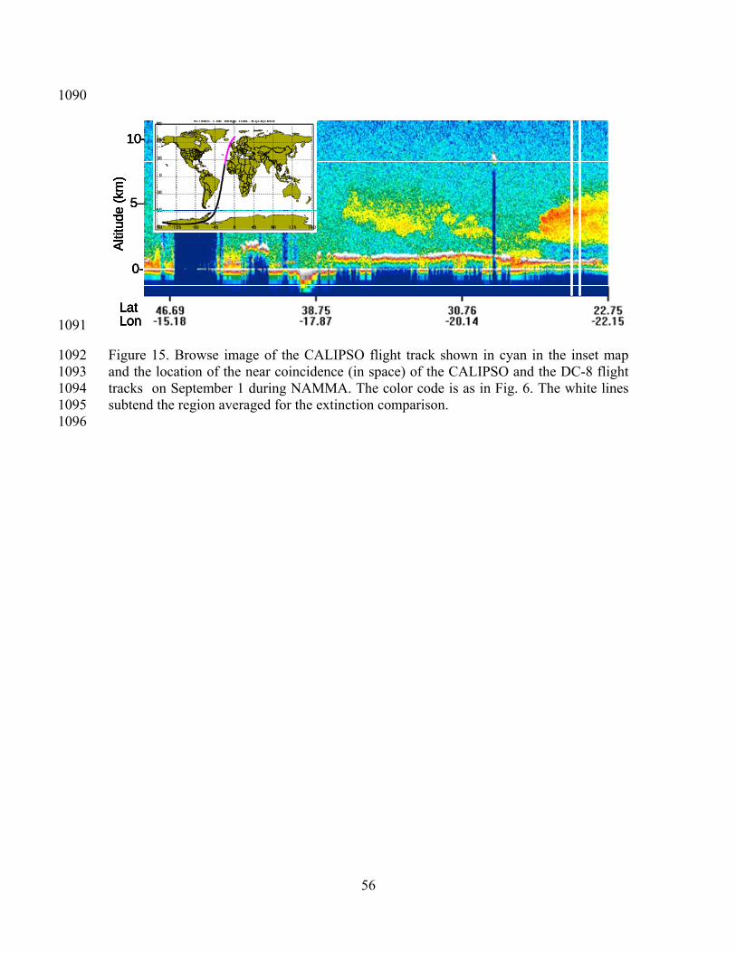
56

1090

10-

5–

0-

Alti

tude

(km

)

LatLon

10-

5

0

Alti

tude

(km

)

LatLon

10-

5–

0-

Alti

tude

(km

)

LatLon

10-

5

0

Alti

tude

(km

)

LatLon 1091

Figure 15. Browse image of the CALIPSO flight track shown in cyan in the inset map 1092 and the location of the near coincidence (in space) of the CALIPSO and the DC-8 flight 1093 tracks on September 1 during NAMMA. The color code is as in Fig. 6. The white lines 1094 subtend the region averaged for the extinction comparison. 1095

1096

57

1097

0

2

4

6

8

10

-100 0 100 200 300 400

NAMMA In-Situ (Extinction)CALIPSO (532 nm Extinction)

Alti

tude

(km

)

Extinction (Mm-1)

September 1, 2006

1098

Figure 16. The NAMMA/CALIPSO extinction comparison for Flight 10 on September 1, 1099 2006. Note that the centroid of the layer has shifted upwards by about 1.5 km in between 1100 the CALIPSO measurement and NAMMA sampling. The CALIPSO measurement is ~15 1101 hours earlier and nearly 750 km away. 1102 1103

58

0

2

4

6

8

10

50800

51000

51200

51400

51600

51800

52000

52200

0 10 20 30 40 50 60

S532nm

(sr) N (#/cm3)S1064nm

(sr)A

ltit

ude

(km

)Tim

e (s)

Coarse particle number concentration (N, #/cm3)Extinction to Backscatter Ratio (S sr)

dust layer base

dust layer top

1104

Figure 17. A profile of the 1064 and 532-nm Sa ratios and integrated number distribution 1105 of coarse particles (0.583 um – 6.264 um) taken from a 20-minute segment of the APS 1106 measurements during Flight 4 on August 19, 2006. The dust base and top are shown by 1107 the lines at altitudes of 2.5 km and 4.6 km, respectively. The mean 532-nm and 1064-nm 1108 Sa ratios for the layer is 34.3 ± 2.0 sr and 50.2 ± 5.7 sr, respectively. 1109 1110

59

 

1

2

3

4

5

6

54000 54500 55000 55500 56000 56500 57000 57500 58000

Alti

tude

(km

)

Time (s)

(a)

(b)

54500

55000

55500

56000

56500

57000

57500

0 20 40 60 80 100

N (#/cm3)S

532 nm (sr)

S1064 nm

(sr)

Tim

e (s

)

Coarse Particle Number Concentration (#/cm3)Extinction to Backscatter Ratio (S

a sr)

1

2

3

4

5

6

54000 54500 55000 55500 56000 56500 57000 57500 58000

Alti

tude

(km

)

Time (s)

(a)

(b)

54500

55000

55500

56000

56500

57000

57500

0 20 40 60 80 100

N (#/cm3)S

532 nm (sr)

S1064 nm

(sr)

Tim

e (s

)

Coarse Particle Number Concentration (#/cm3)Extinction to Backscatter Ratio (S

a sr)

1111

Figure 18. (a) The flight track of the DC-8 on August 25, 2006. The straight and nearly 1112 level portion is through a dust layer at ~2 km. (b) The calculated 532- and 1064-nm Sa 1113 ratios and coarse number particle concentration for the straight and level portion of this 1114 flight. 1115 1116

60

0

0.5

1

1.5

2

2.5

3

65340

65360

65380

65400

65420

65440

65460

65480

-10 0 10 20 30 40 50 60

S532nm

(sr)

S1064nm

(sr)

N (#/cm3)

Alt

itud

e (k

m)

Time (s)

Coarse particle number concentration (N, #/cm3)Extinction to Backscatter Ratio (S sr)

1117

Figure 19. A profile of the 1064- and 532 –nm Sa ratios, and integrated number 1118 distribution of coarse particles during Flight 8 on Aug. 26, 2006. The mean 532-nm and 1119 1064-nm Sa ratios for the layer is 39.0 ± 1.5 sr and 45.9 ± 2.2 sr, respectively. 1120

1121

61

1122

1.125

1.5

1.875

2.25

68800 69000 69200 69400 69600 69800

(a)A

ltit

ude

(km

)

Time (s)

Leg 1

Leg 3Leg 2

Leg 4

Flight path

1123

68800

68900

69000

69100

69200

69300

69400

25 30 35 40 45 50 55 60

08262006 Straight and Level Leg 1

S532 nm

S1064 nm N (#/cm3)

Tim

e (s

ecs)

Coarse particle number concentration (N, #/cm3)Extinction to Backscatter Ratio (S sr)

(b)

1124

1125

62

1.21.281.361.441.521.6

1.681.761.84

1.91.95

22.05

2.12.152.2

2.25

69760

69780

69800

69820

69840

69260

69270

69280

69290

69300

69310

69320

0 10 20 30 40 50 60 70

08262006 Leg 2

S532 nm

S1064 nm

N (#/cm3)

Alt

itud

e (k

m) Tim

e (secs)

Coarse particle number concentration (N, #/cm3)Extinction to Backscatter Ratio (S sr)

08262006 Leg 4

(c)

1126

1127

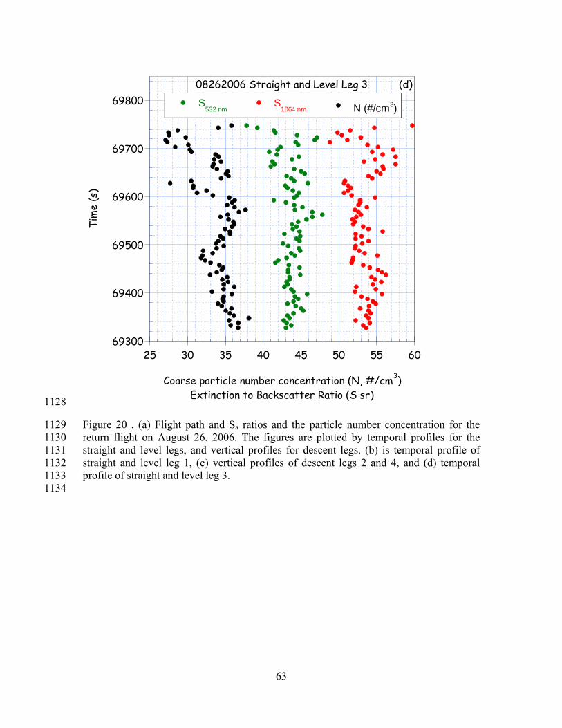
63

69300

69400

69500

69600

69700

69800

25 30 35 40 45 50 55 60

08262006 Straight and Level Leg 3

S532 nm

S1064 nm N (#/cm3)

Tim

e (s

)

Coarse particle number concentration (N, #/cm3)Extinction to Backscatter Ratio (S sr)

(d)

1128

Figure 20 . (a) Flight path and Sa ratios and the particle number concentration for the 1129 return flight on August 26, 2006. The figures are plotted by temporal profiles for the 1130 straight and level legs, and vertical profiles for descent legs. (b) is temporal profile of 1131 straight and level leg 1, (c) vertical profiles of descent legs 2 and 4, and (d) temporal 1132 profile of straight and level leg 3. 1133 1134

64

0

1

2

3

4

5

6

7

57250 57500 57750 58000 58250 58500 58750 59000

Alt

itud

e (k

m)

Time (secs)

0.8

1.6

2.4

3.2

4

4.8

5.657100

57200

57300

57400

57500

57600

57700

57800

57900

0 10 20 30 40 50 60 70

(b) Descent Leg

S53 2 nm

S10 64 nm

N (#/cm3)

Alt

itud

e (k

m) T

ime (secs)

Coarse particle number concentration (N, #/cm3)Extinction to Backscatter Ratio (S sr)

0.8

1.6

2.4

3.2

4

4.8

5.6

58400

58500

58600

58700

58800

58900

59000

59100

0 10 20 30 40 50 60 70

(c) Ascent LegS532 nm

S1064 n m

N (#/cm3)

Alt

itud

e (k

m) T

ime (secs)

Coarse particle number concentration (N, #/cm3)Extinction to Backscatter Ratio (S sr)

(a) Flight path

0

1

2

3

4

5

6

7

57250 57500 57750 58000 58250 58500 58750 59000

Alt

itud

e (k

m)

Time (secs)

0.8

1.6

2.4

3.2

4

4.8

5.657100

57200

57300

57400

57500

57600

57700

57800

57900

0 10 20 30 40 50 60 70

(b) Descent Leg

S53 2 nm

S10 64 nm

N (#/cm3)

Alt

itud

e (k

m) T

ime (secs)

Coarse particle number concentration (N, #/cm3)Extinction to Backscatter Ratio (S sr)

0.8

1.6

2.4

3.2

4

4.8

5.6

58400

58500

58600

58700

58800

58900

59000

59100

0 10 20 30 40 50 60 70

(c) Ascent LegS532 nm

S1064 n m

N (#/cm3)

Alt

itud

e (k

m) T

ime (secs)

Coarse particle number concentration (N, #/cm3)Extinction to Backscatter Ratio (S sr)

(a) Flight path

1135

Figure 21.The (a) flight path and Sa ratios and the particle number concentration for the 1136 flight on August 20, 2006 plotted vertical profiles of (b) the descent leg and (c) the ascent 1137 leg. 1138

1139

65

30 35 40 45 50 55 60 65 700

0.02

0.04

0.06

0.08

0.1

0.12

Extinction/Backscatter Ratio (sr)

Fra

ctio

na

l Fre

qu

en

cy

532 nm

1064 nm

1140

Figure 22. An ensemble of all the Sa ratio estimates (~1100 records) based on the 1141 NAMMA in-situ size distributions of dust layers and T-Matrix calculations. The average 1142 Sa ratios are 39.1 ± 3.5 sr and 50.0 ± 4 sr at 532 nm and 1064 nm, respectively 1143

1144

66

1145

0.8 1 1.2 1.4 1.6 1.8 20

0.02

0.04

0.06

0.08

0.1

0.12

0.14

0.16

Ratio of Extinction/Backscatter Ratios

Fra

ctio

na

l Fre

qu

en

cy

1146

Figure 23. The ratio of the Sa ratios [Sa (1064 nm)/Sa (532 nm)] derived from the size 1147 distribution data used for this study. 1148 1149 1150

1151

67

1152

20 40 60 80 1000

0.05

0.1

0.15

0.2

0.25

0.3

0.35

0.4

Extinction/Backscatter Ratio (sr)

Frac

tion

al F

requ

ency

532 nm1064 nm

1153 1154 Figure 24. The distribution of the Sa ratio calculated from a Latin Hypercube Sample 1155 (LHS) of 500 events bounded by the ranges shown in Table 3. The normal means (± 1 1156 standard deviation) of the 532- and 1064-nm Sa ratios are 39.4 ± 5.9 sr and 56.5 ± 16.5 sr, 1157 respectively. 1158 1159

68

532-

nm L

idar

Rat

io (s

r)

Imaginary Part of the Refractive Index

0.001 0.002 0.003 0.004 0.00525

30

35

40

45

50

55

60

65

0

5

10

15

20

0.001 0.002 0.003 0.004 0.005

30

40

50

60

70

80

90

0

1

2

3

4

5

6

7

8

9

10

11

1064

-nm

Lid

ar R

atio

(sr)

Imaginary Part of the Refractive Index

1.46 1.47 1.48 1.49 1.5 1.51 1.52 1.53 1.5425

30

35

40

45

50

55

60

65

0

2

4

6

8

10

12

14

16

532-

nm L

idar

Rat

io (s

r)

Real Part of the Refractive Index

1.46 1.47 1.48 1.49 1.5 1.51 1.52 1.53 1.54

30

40

50

60

70

80

90

0

2

4

6

8

10

12

1064

-nm

Lid

ar R

atio

(sr)

Real Part of the Refractive Index

(a)

(c)

(b)

(d)

1160

Figure 25. Two-dimensional frequency plots showing the variation of the lidar ratios with 1161 real and imaginary parts of the complex refractive indices for 500 randomly generated 1162 events discussed in section 6. 1163 1164 1165