Embed Size (px)
Citation preview
Exponential Smoothing 1Ardavan Asef-Vaziri 6/4/2009
Forecasting-2
Chapter 7Demand Forecastingin a Supply Chain
Forecasting -2Exponential Smoothing
Ardavan Asef-Vaziri
Based on Operations management: Stevenson
Operations Management: Jacobs and ChaseSupply Chain Management: Chopra and Meindl
Exponential Smoothing 2Ardavan Asef-Vaziri 6/4/2009
Forecasting-2
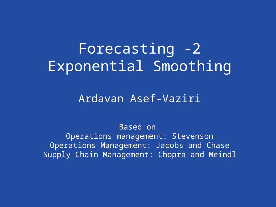
Time Series Methods
Moving Average Discard old records
Assign same weight for recent records
Assign different weights Weighted moving average
3211 ttttt AAAAF 3211 1.02.03.04.0 ttttt AAAAF
Exponential Smoothing

Exponential Smoothing 3Ardavan Asef-Vaziri 6/4/2009
Forecasting-2
Exponential Smoothing
)(α1 tttt FAFF
ttt AFF α)α1(1
tttt FAFF αα1

Exponential Smoothing 4Ardavan Asef-Vaziri 6/4/2009
Forecasting-2
Exponential Smoothing
α=0.2 tAtFt
1100100
A1 F2
2
100
Since I have no information for F1, I just enter A1 which is 100. Alternatively we may assume the average of all available data as our forecast for period 1.
150
F3 =(1-α)F2 + α A2
F3 =0.8(100) + 0.2(150)
F3 =80 + 30 = 110
3
110
F2 & A2 F3
A1 F2 A1 & A2 F3
F3 =(1-α)F2 + α A2

Exponential Smoothing 5Ardavan Asef-Vaziri 6/4/2009
Forecasting-2
Exponential Smoothing
α=0.2
tAtFt
1100100
F4 =(1-α)F3 + α A3
F4 =0.8(110) + 0.2(120)
F4 =88 + 24 = 112
A3 & F3 F4
A1 & A2 F3 A1& A2 & A3 F4
2150100
3
110
4
112120
F4 =(1-α)F3 + α A3

Exponential Smoothing 6Ardavan Asef-Vaziri 6/4/2009
Forecasting-2
Example: Forecast for week 9 using a = 0.1
Week Demand Forecast
1 200
2 250 200
3 175
4 186
5 225
6 285
7 305
8 190
205250*1.0200*9.01 223 AFF

Exponential Smoothing 7Ardavan Asef-Vaziri 6/4/2009
Forecasting-2
Week 4
Week Demand Forecast
1 200
2 250 200
3 175 205
4 186
5 225
6 285
7 305
8 190
202175*1.0205*9.01 334 AFF

Exponential Smoothing 8Ardavan Asef-Vaziri 6/4/2009
Forecasting-2
Exponential Smoothing
Week Demand Forecast
1 200
2 250 200
3 175 205
4 186 202
5 225 200
6 285 203
7 305 211
8 190 220

Exponential Smoothing 9Ardavan Asef-Vaziri 6/4/2009
Forecasting-2
Two important questions
How to choose a? Large or Small When does it work? When does it not?
What is better exponential smoothing
OR moving average?

Exponential Smoothing 10Ardavan Asef-Vaziri 6/4/2009
Forecasting-2
The Same Example: a = 0.4
Week Demand Forecast
1 200
2 250 200
3 175 220
4 186 202
5 225 196
6 285 207
7 305 238
8 190 265

Exponential Smoothing 11Ardavan Asef-Vaziri 6/4/2009
Forecasting-2
Comparison
0
50
100
150
200
250
300
350
1 2 3 4 5 6 7 8
week
Demand
alpha = 0.1
alpha = 0.4
Exponential Smoothing 12Ardavan Asef-Vaziri 6/4/2009
Forecasting-2
Comparison
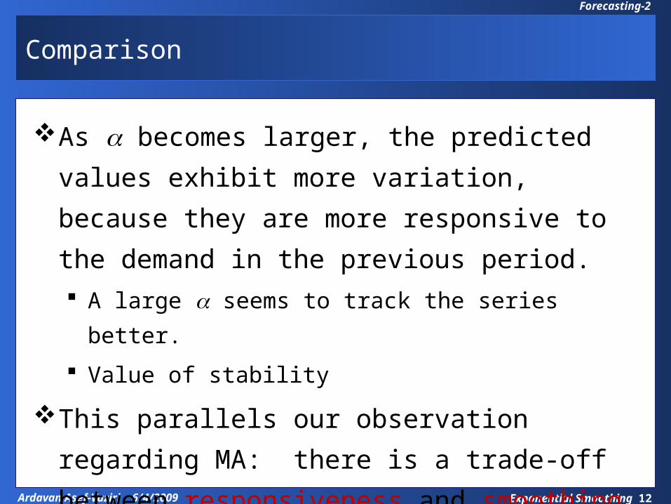
As a becomes larger, the predicted values
exhibit more variation, because they are
more responsive to the demand in the
previous period. A large a seems to track the series better.
Value of stability
This parallels our observation regarding MA:
there is a trade-off between responsiveness
and smoothing out demand fluctuations.

Exponential Smoothing 13Ardavan Asef-Vaziri 6/4/2009
Forecasting-2
Comparison
Week DemandForecast for
0.1 alpha ADForecast for 0.4
alpha AD
1 200
2 250 200.00 50.00 200.00 50.00
3 175 205.00 30.00 220.00 45.00
4 186 202.00 16.00 202.00 16.00
5 225 200.40 24.60 195.60 29.40
6 285 202.86 82.14 207.36 77.64
7 305 211.07 93.93 238.42 66.58
8 190 220.47 30.47 265.05 75.05
46.73 51.38
Choose the forecast with lower MAD.

Exponential Smoothing 14Ardavan Asef-Vaziri 6/4/2009
Forecasting-2
Which a to choose?
In general want to calculate MAD for many
different values of a and choose the one
with the lowest MAD.
Same idea to determine if Exponential
Smoothing or Moving Average is preferred.
Note that one advantage of exponential
smoothing requires less data storage to
implement.

Exponential Smoothing 15Ardavan Asef-Vaziri 6/4/2009
Forecasting-2
All Pieces of Data are Taken into Account in ES
Ft = a At–1 + (1 – a) Ft–1
Ft–1 = a At–2 + (1 – a) Ft–2
Ft = aAt–1+(1–a)aAt–2+(1–a)2Ft–2
Ft–2 = a At–3 + (1 – a) Ft–3
Ft = aAt–1+(1–a)aAt–2+(1–a)2a At–3 + (1 – a) 3 Ft–3
= aAt–1+(1–a)aAt–2+(1–a)2aAt–3 +(1–a)3aAt–4
+(1–a)4aAt–5+(1–a)5aAt–6 +(1–a)6aAt–7+…
A large number of data are taken into account– All data are taken
into account in ES.

Exponential Smoothing 16Ardavan Asef-Vaziri 6/4/2009
Forecasting-2
What is better? Exponential Smoothing or Moving Average
Age of data in moving average is (1+ n)/2 .Age of data in exponential smoothing is about 1/
a.1n)/2 = 1/ a a = 2/(n+1)If we set a = 2/(n +1) , then moving average and
exponential smoothing are approximately equivalent. It does not mean that the two models have
the same forecasts. The variances of the errors are identical.
Exponential Smoothing 17Ardavan Asef-Vaziri 6/4/2009
Forecasting-2
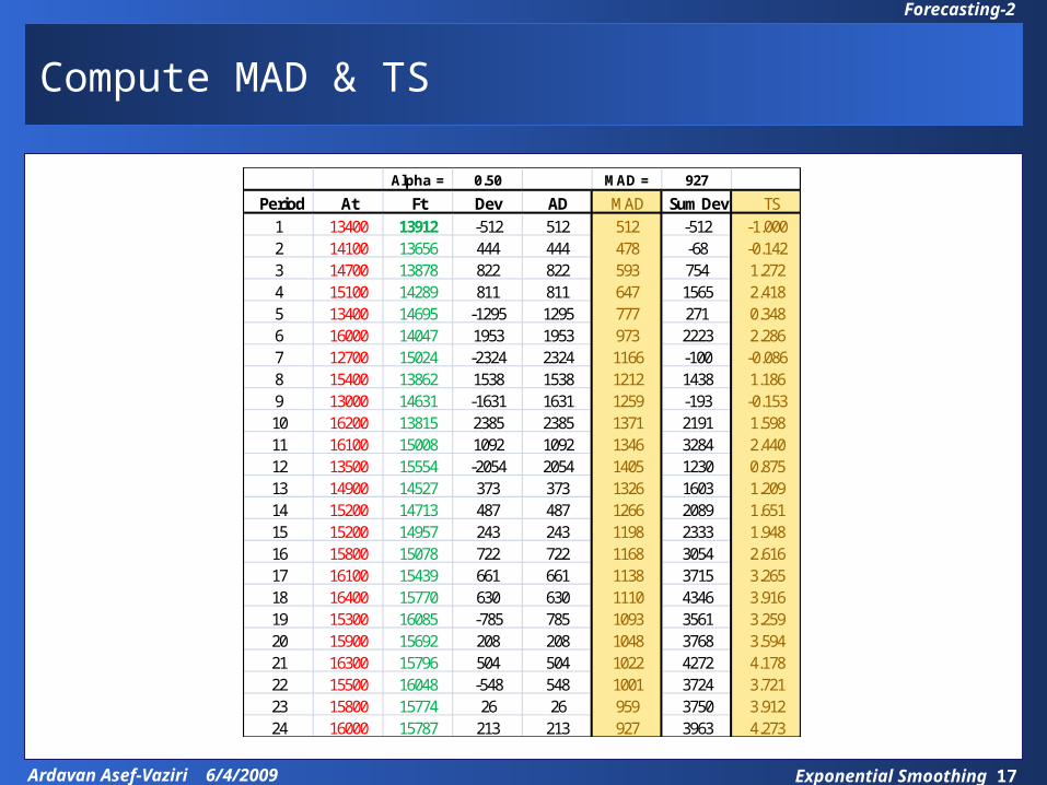
Compute MAD & TS
Alpha = 0.50 MAD = 927
Period At Ft Dev AD MAD Sum Dev TS1 13400 13912 -512 512 512 -512 -1.0002 14100 13656 444 444 478 -68 -0.1423 14700 13878 822 822 593 754 1.2724 15100 14289 811 811 647 1565 2.4185 13400 14695 -1295 1295 777 271 0.3486 16000 14047 1953 1953 973 2223 2.2867 12700 15024 -2324 2324 1166 -100 -0.0868 15400 13862 1538 1538 1212 1438 1.1869 13000 14631 -1631 1631 1259 -193 -0.15310 16200 13815 2385 2385 1371 2191 1.59811 16100 15008 1092 1092 1346 3284 2.44012 13500 15554 -2054 2054 1405 1230 0.87513 14900 14527 373 373 1326 1603 1.20914 15200 14713 487 487 1266 2089 1.65115 15200 14957 243 243 1198 2333 1.94816 15800 15078 722 722 1168 3054 2.61617 16100 15439 661 661 1138 3715 3.26518 16400 15770 630 630 1110 4346 3.91619 15300 16085 -785 785 1093 3561 3.25920 15900 15692 208 208 1048 3768 3.59421 16300 15796 504 504 1022 4272 4.17822 15500 16048 -548 548 1001 3724 3.72123 15800 15774 26 26 959 3750 3.91224 16000 15787 213 213 927 3963 4.273

Exponential Smoothing 18Ardavan Asef-Vaziri 6/4/2009
Forecasting-2
Data Table Excel
9270.1 10170.2 8970.3 8860.4 9010.5 9270.6 9600.7 9970.8 10360.9 1078
1 1130
9270.1 10170.2 8970.3 8860.4 9010.5 9270.6 9600.7 9970.8 10360.9 1078
1 1130 886
Data, what if, Data table
Min, conditional formatting
Alpha = 0.50 MAD = 927
Period At Ft Dev AD MAD Sum Dev TS1 13400 13912 -512 512 512 -512 -1.0002 14100 13656 444 444 478 -68 -0.1423 14700 13878 822 822 593 754 1.2724 15100 14289 811 811 647 1565 2.4185 13400 14695 -1295 1295 777 271 0.3486 16000 14047 1953 1953 973 2223 2.2867 12700 15024 -2324 2324 1166 -100 -0.0868 15400 13862 1538 1538 1212 1438 1.1869 13000 14631 -1631 1631 1259 -193 -0.15310 16200 13815 2385 2385 1371 2191 1.59811 16100 15008 1092 1092 1346 3284 2.44012 13500 15554 -2054 2054 1405 1230 0.87513 14900 14527 373 373 1326 1603 1.20914 15200 14713 487 487 1266 2089 1.65115 15200 14957 243 243 1198 2333 1.94816 15800 15078 722 722 1168 3054 2.61617 16100 15439 661 661 1138 3715 3.26518 16400 15770 630 630 1110 4346 3.91619 15300 16085 -785 785 1093 3561 3.25920 15900 15692 208 208 1048 3768 3.59421 16300 15796 504 504 1022 4272 4.17822 15500 16048 -548 548 1001 3724 3.72123 15800 15774 26 26 959 3750 3.91224 16000 15787 213 213 927 3963 4.273
9270.10.20.30.40.50.60.70.80.9
1 This is a one variable Data Table

Exponential Smoothing 19Ardavan Asef-Vaziri 6/4/2009
Forecasting-2
Office Button
Exponential Smoothing 20Ardavan Asef-Vaziri 6/4/2009
Forecasting-2
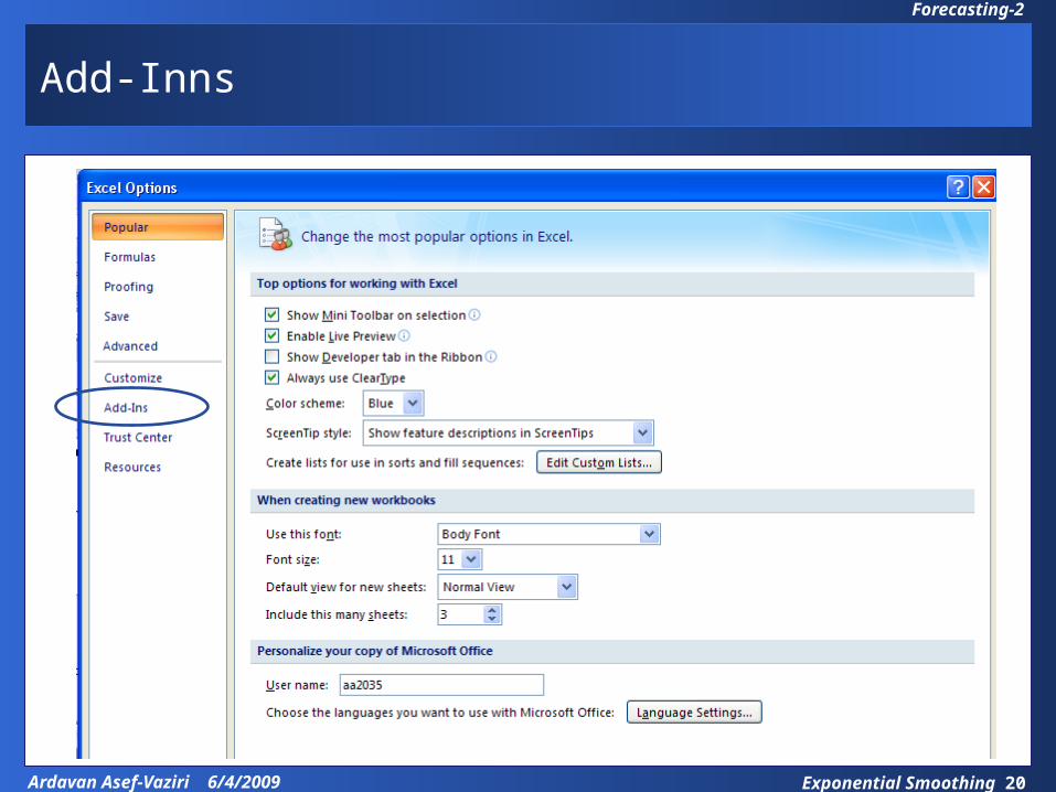
Add-Inns

Exponential Smoothing 21Ardavan Asef-Vaziri 6/4/2009
Forecasting-2
Not OK, but GO, then Check Mark Solver

Exponential Smoothing 22Ardavan Asef-Vaziri 6/4/2009
Forecasting-2
Data Tab/ Solver

Exponential Smoothing 23Ardavan Asef-Vaziri 6/4/2009
Forecasting-2
Target Cell/Changing Cells

Exponential Smoothing 24Ardavan Asef-Vaziri 6/4/2009
Forecasting-2
Optimal a Minimal MAD

Exponential Smoothing 25Ardavan Asef-Vaziri 6/4/2009
Forecasting-2
NOTE – The following pages are not recorded
Note: The following discussion – from the next
page up to the end of this set of slides – are
not recorded.

Exponential Smoothing 26Ardavan Asef-Vaziri 6/4/2009
Forecasting-2
Measures of Forecast Error; Additional Indices
Error: difference between predicted value
and actual value (E)
Mean Absolute Deviation (MAD)
Tracking Signal (TS)
Mean Square Error (MSE)
Mean Absolute Percentage Error (MAPE)

Exponential Smoothing 27Ardavan Asef-Vaziri 6/4/2009
Forecasting-2
7-1-27
Measures of Forecast Error
nsObservatio of # (MAD)Deviation AbsoluteMean tE
nsObservatio of # (MSE)Error SquaredMean
2 tE
nsObservatio of #
100
)Error(MAPE Percentage AbsoluteMean
t
t
A
E
Error ofDeviation Standard estimatean is 1.25MAD
Error ofDeviation Standard estimateanother also is MSE


![Forecasting using - Rob J Hyndman exponential smoothing Forecasting using R Simple exponential smoothing 9 animation by animate[2012/05/24] Simple exponential smoothing Optimization](https://img.dokumen.tips/doc/110x75/5aae58377f8b9a07498bfac5/forecasting-using-rob-j-hyndman-exponential-smoothing-forecasting-using-r-simple.jpg)