Exponential Smoothing

INSR 260, Spring 2009Bob Stine

1

Overview Smoothing

Exponential smoothing

Model behind exponential smoothingForecasts and estimatesHidden state model

Diagnostic: residual plots

Examples! ! ! ! (from Bowerman, Ch 8,9)Cod catchPaper sales

2

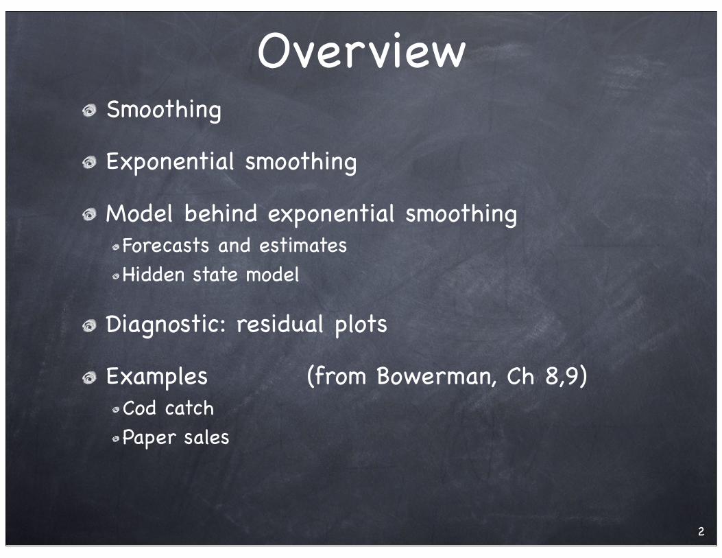
SmoothingHeuristic! ! Data = Pattern + Noise

Pattern is slowly changing, predictableNoise may have short-term dependence, but by-and-large is irregular and unpredictable

IdeaIsolate the pattern from the noise by averaging data that are nearby in time.

Noise should mostly cancel out, revealing the patternExample: moving averages

Example: JMP’s spline smoothing uses different weights3

st = yt!w+···+yt!1+yt+yt+1+···+yt+w

2w+1

Simple Exponential SmoothMoving averages have a problem

Not useful for prediction:Smooth st depends upon observations in the future.Cannot compute near the ends of the data series

Exponential smoothing is one-sidedAverage of current and prior valuesRecent values are more heavily weighted than Tuning parameter α = (1-w) controls weights (0≤w<1)

Two expressions for the smoothed value

4

!t = yt+wyt!1+w2yt!2+···1+w+w2+···

Weighted average Predictor/Corrector

!t =yt

1 + w + w2 + · · · +w(yt!1 + wyt!2 + · · ·

1 + w + w2 + · · ·= (1! w)yt + w!t!1

= "yt + (1! ")!t!1

= !t!1 + "(yt ! !t!1)

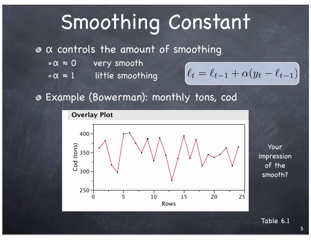
Smoothing Constantα controls the amount of smoothingα ≈ 0 very smoothα ≈ 1 little smoothing

Example (Bowerman): monthly tons, cod

5

250

300

350

400

Cod (

tons)

0 5 10 15 20 25

Rows

Overlay Plot

Your impression

of the smooth?

!t = !t!1 + "(yt ! !t!1)

Table 6.1

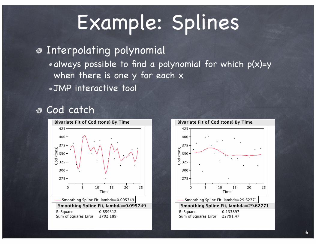
Example: SplinesInterpolating polynomial

always possible to find a polynomial for which p(x)=y when there is one y for each xJMP interactive tool

Cod catch

6

275

300

325

350

375

400

425

Cod (

tons)

0 5 10 15 20 25

Time

Smoothing Spline Fit, lambda=0.095749

R-Square

Sum of Squares Error

0.859312

3702.189

Smoothing Spline Fit, lambda=0.095749

Bivariate Fit of Cod (tons) By Time

275

300

325

350

375

400

425

Cod (

tons)

0 5 10 15 20 25

Time

Smoothing Spline Fit, lambda=29.62771

R-Square

Sum of Squares Error

0.133897

22791.47

Smoothing Spline Fit, lambda=29.62771

Bivariate Fit of Cod (tons) By Time

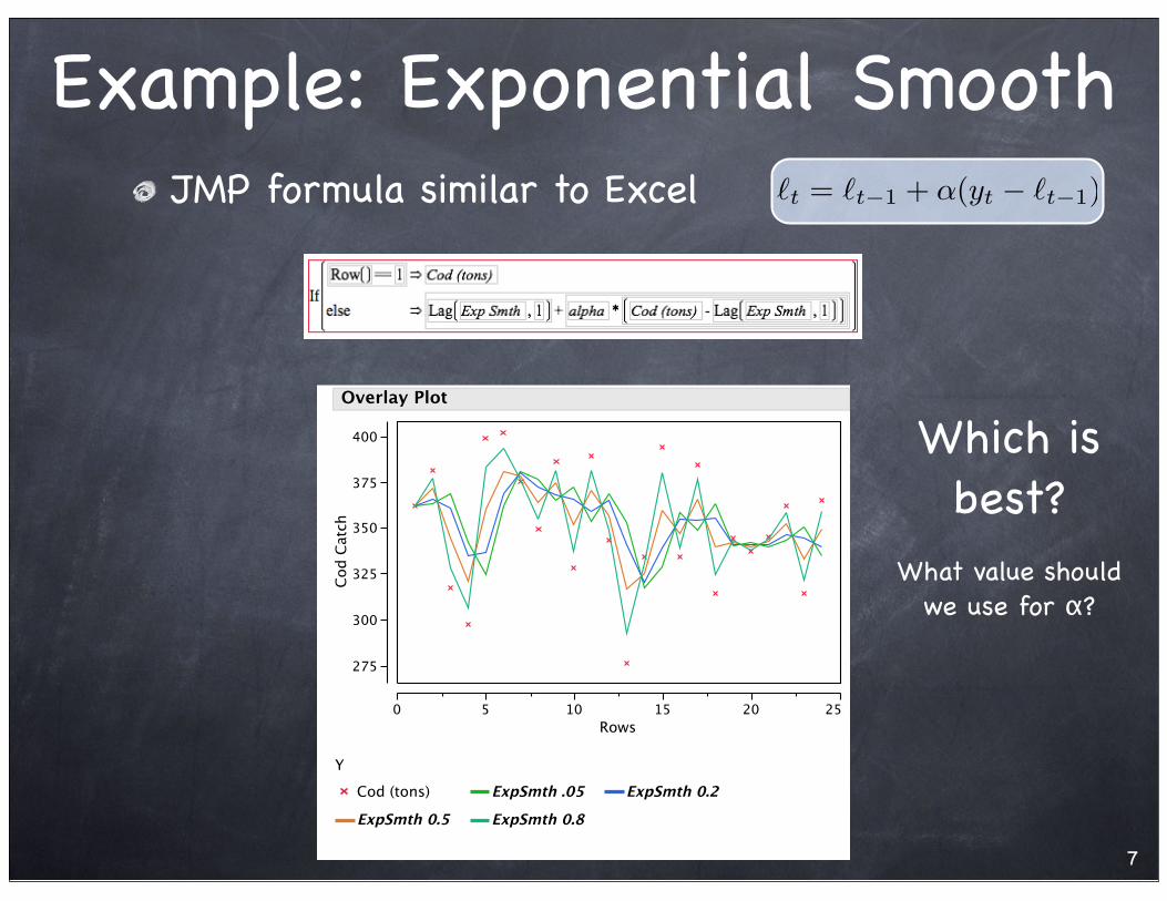
Example: Exponential SmoothJMP formula similar to Excel

7

275

300

325

350

375

400

Cod C

atc

h

0 5 10 15 20 25

Rows

Overlay Plot

Y

Cod (tons) ExpSmth .05 ExpSmth 0.2

ExpSmth 0.5 ExpSmth 0.8

Which is best?

!t = !t!1 + "(yt ! !t!1)

What value should we use for α?

ModelNeed statistical model to

Express source of randomness, uncertaintyChoose an optimal estimate for αDefine predictor and quantify probable accuracy

Want to have prediction intervals for exponential smoothing

Latent variable model (“state-space models”)Assume each observation has mean Lt-1 ! ! ! ! ! ! ! yt = Lt-1 + εtMean values fluctuate over time! ! ! ! ! ! ! Lt = Lt-1 + α εtDiscussion

Lt is the state and is not observedIf α = 0, Lt is constantIf α = 1, Lt is just as variable as the data

8

εt ~ N(0,σ2)

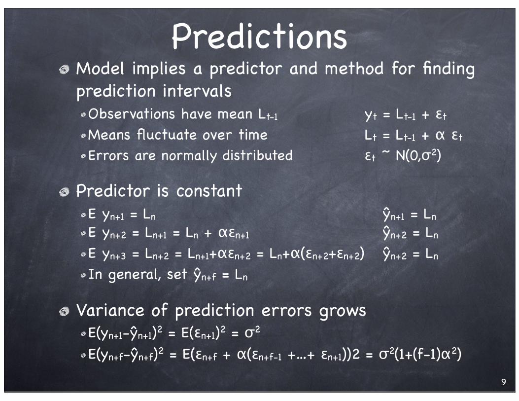
PredictionsModel implies a predictor and method for finding prediction intervals

Observations have mean Lt-1! ! ! ! ! yt = Lt-1 + εtMeans fluctuate over time!! ! ! ! ! Lt = Lt-1 + α εtErrors are normally distributed! ! ! ! εt ~ N(0,σ2)

Predictor is constantE yn+1 = Ln! ! ! ! ! ! ! ! ! ! ! ! ! ŷn+1 = Ln E yn+2 = Ln+1 = Ln + αεn+1!! ! ! ! ! ! ! ŷn+2 = Ln E yn+3 = Ln+2 = Ln+1+αεn+2 = Ln+α(εn+2+εn+2)!! ŷn+2 = Ln In general, set ŷn+f = Ln

Variance of prediction errors growsE(yn+1-ŷn+1)2 = E(εn+1)2 = σ2

E(yn+f-ŷn+f)2 = E(εn+f + α(εn+f-1 +…+ εn+1))2 = σ2(1+(f-1)α2)

9

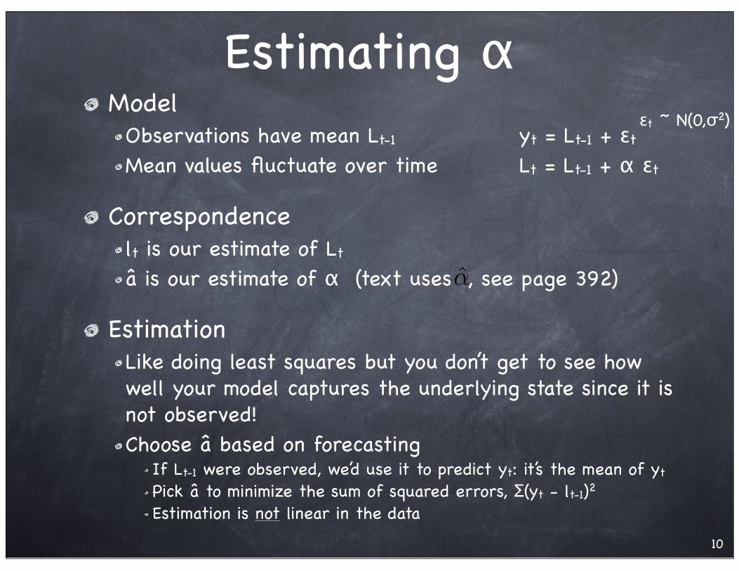
Estimating α Model

Observations have mean Lt-1! ! ! ! ! yt = Lt-1 + εtMean values fluctuate over time!! ! ! Lt = Lt-1 + α εt

Correspondencelt is our estimate of Lt

â is our estimate of α (text uses , see page 392)

EstimationLike doing least squares but you don’t get to see how well your model captures the underlying state since it is not observed!Choose â based on forecasting

If Lt-1 were observed, we’d use it to predict yt: it’s the mean of yt

Pick â to minimize the sum of squared errors, Σ(yt - lt-1)2Estimation is not linear in the data

10

εt ~ N(0,σ2)

!̂

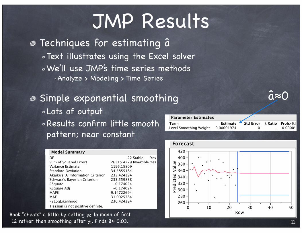
JMP ResultsTechniques for estimating â

Text illustrates using the Excel solverWe’ll use JMP’s time series methods

Analyze > Modeling > Time Series

Simple exponential smoothingLots of outputResults confirm little smoothpattern; near constant

11

DF

Sum of Squared Errors

Variance Estimate

Standard Deviation

Akaike's 'A' Information Criterion

Schwarz's Bayesian Criterion

RSquare

RSquare Adj

MAPE

MAE

-2LogLikelihood

22

26315.4779

1196.15809

34.5855184

232.424394

233.559888

-0.174024

-0.174024

9.14722694

31.0025784

230.424394

Stable

Invertible

Yes

Yes

Hessian is not positive definite.

Model Summary

Level Smoothing Weight

Term

0.00001974

Estimate

0

Std Error

.

t Ratio

0.0000*Prob>|t|

Parameter Estimates

260

280

300

320

340

360

380

400

420

Predic

ted V

alu

e

0 10 20 30 40 50

Row

Forecast

â≈0

Book “cheats” a little by setting y0 to mean of first 12 rather than smoothing after y1. Finds â≈ 0.03.

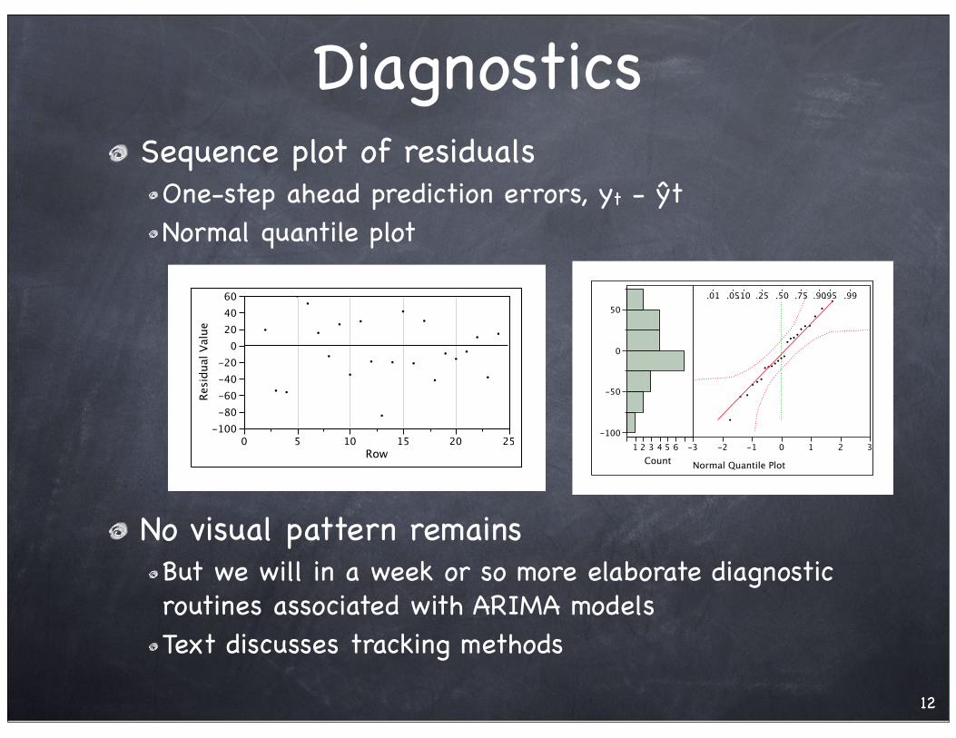
DiagnosticsSequence plot of residuals

One-step ahead prediction errors, yt - ŷtNormal quantile plot

No visual pattern remainsBut we will in a week or so more elaborate diagnostic routines associated with ARIMA modelsText discusses tracking methods

12

-100

-80

-60

-40

-20

0

20

40

60

Resid

ual V

alu

e

0 5 10 15 20 25

Row

-100

-50

0

50

1 2 3 4 5 6

Count

.01 .05.10 .25 .50 .75 .90.95 .99

-3 -2 -1 0 1 2 3

Normal Quantile Plot

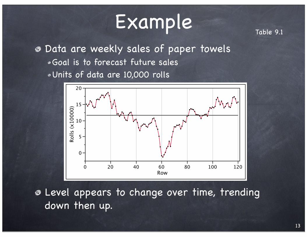
ExampleData are weekly sales of paper towels

Goal is to forecast future salesUnits of data are 10,000 rolls

Level appears to change over time, trending down then up.

13

Table 9.1

0

5

10

15

20

Rolls (

x10000)

0 20 40 60 80 100 120

Row

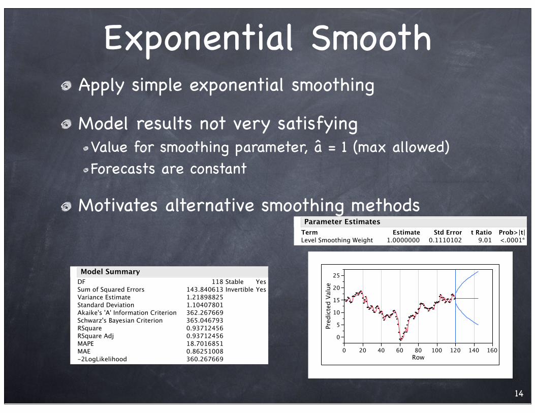
Exponential SmoothApply simple exponential smoothing

Model results not very satisfyingValue for smoothing parameter, â = 1 (max allowed)Forecasts are constant

Motivates alternative smoothing methods

14

0

5

10

15

20

25

Predic

ted V

alu

e

0 20 40 60 80 100 120 140 160

Row

Level Smoothing Weight

Term

1.0000000

Estimate

0.1110102

Std Error

9.01

t Ratio

<.0001*Prob>|t|

Parameter Estimates

DF

Sum of Squared Errors

Variance Estimate

Standard Deviation

Akaike's 'A' Information Criterion

Schwarz's Bayesian Criterion

RSquare

RSquare Adj

MAPE

MAE

-2LogLikelihood

118

143.840613

1.21898825

1.10407801

362.267669

365.046793

0.93712456

0.93712456

18.7016851

0.86251008

360.267669

Stable

Invertible

Yes

Yes

Model Summary

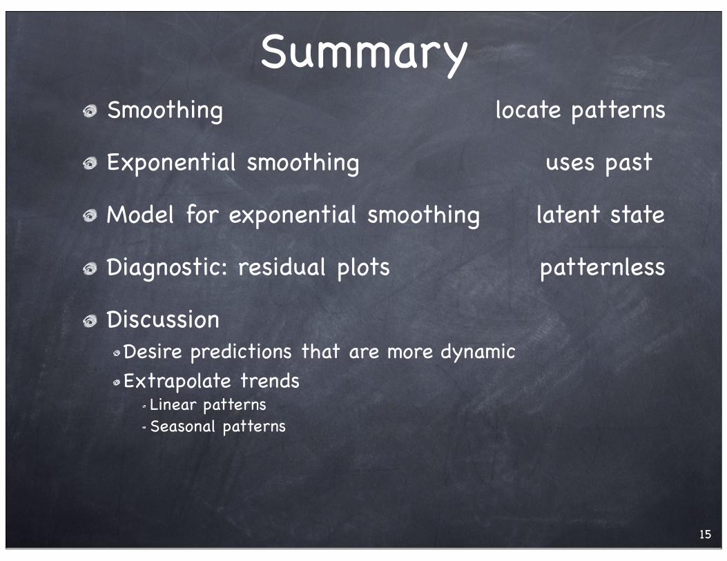
SummarySmoothing!! ! ! ! ! ! ! ! ! ! locate patterns

Exponential smoothing!! ! ! ! ! ! ! uses past

Model for exponential smoothing!! ! latent state

Diagnostic: residual plots! ! ! ! ! patternless

DiscussionDesire predictions that are more dynamicExtrapolate trends

Linear patternsSeasonal patterns

15