Exploiting temporal consistency for real-time video depth estimation∗

Haokui Zhang1, Chunhua Shen2, Ying Li1, Yuanzhouhan Cao2, Yu Liu2, Youliang Yan3

1Northwestern Polytechnical University 2University of Adelaide 3Noah’s Ark Lab, Huawei

Abstract

Accuracy of depth estimation from static images has

been significantly improved recently, by exploiting hierar-

chical features from deep convolutional neural networks

(CNNs). Compared with static images, vast information ex-

ists among video frames and can be exploited to improve

the depth estimation performance. In this work, we focus

on exploring temporal information from monocular videos

for depth estimation. Specifically, we take the advantage of

convolutional long short-term memory (CLSTM) and pro-

pose a novel spatial-temporal CSLTM (ST-CLSTM) struc-

ture. Our ST-CLSTM structure can capture not only the spa-

tial features but also the temporal correlations/consistency

among consecutive video frames with negligible increase in

computational cost. Additionally, in order to maintain the

temporal consistency among the estimated depth frames, we

apply the generative adversarial learning scheme and de-

sign a temporal consistency loss. The temporal consistency

loss is combined with the spatial loss to update the model in

an end-to-end fashion. By taking advantage of the temporal

information, we build a video depth estimation framework

that runs in real-time and generates visually pleasant re-

sults. Moreover, our approach is flexible and can be gener-

alized to most existing depth estimation frameworks. Code

is available at: https://tinyurl.com/STCLSTM

1. Introduction

Benefiting from the powerful convolutional neural net-

works (CNNs), some recent methods [47, 10, 30, 9, 21]

have achieved outstanding performance on depth estimation

from monocular static images. The success of these meth-

ods is based on the deeply stacked network structures and

large amount of training data. For instance, the state-of-

the-art depth estimation model DORN [10] has more than

one hundred of convolution layers, the high computational

cost may hamper it from practical applications. However,

in some scenarios such as automatic driving [2] and robots

navigation [35], estimating of depths in real-time is re-

∗Work was done when H. Zhang was visiting University of Adelaide.

Correspondence should be addressed to C. Shen and Y. Li.

quired. Directly extend existing methods from static image

to video sequence is not feasible because of the excessive

computational cost. In addition, sequential frames which

contain rich temporal information are usually provided in

such scenarios. The existing methods fail to take the tem-

poral information into consideration.

In this work, we exploit temporal information from

videos by making use of the convolutional long short-term

memory (CLSTM) and the generative adversarial networks

(GANs), and propose a real-time depth estimation frame-

work. We illustrate our proposed framework in Fig. 1.

It consists of three main parts: 1) spatial features extrac-

tion part; 2) temporal correlations collection part and 3)

spatial-temporal loss calculation part. The spatial features

extraction part and the temporal correlations collection part

compose our novel spatial-temporal CLSTM (ST-CLSTM)

structure. The spatial features extraction part first takes

as input n continuous frames(

x1, x2, · · · , xn)

and outputs

high level features(

f1, f2, · · · , fn)

. The temporal corre-

lations collection part then takes as input the high-level fea-

tures and outputs depth estimations(

d1, d2, · · · , dn)

. With

the cell and gate modules, the CLSTM can make use of

the cues acquired from the previous frame to reason the

current frame, and thus encode the temporal information.

As for spatial-temporal loss calculation, we first calculate

the spatial loss between the estimated and the ground-truth

depths. In order to further enforce the temporal consistency,

we design a new temporal loss by introducing a generative

adversarial learning scheme. Specifically, we apply a 3D

CNN as the discriminator which takes as input the estimated

and ground-truth depth sequences and outputs the temporal

loss. The temporal loss is combined with the spatial loss and

back propagated through the entire framework to update the

weights in an end-to-end fashion.

To summarize, our main contributions are as follows.

• We propose a novel ST-CLSTM structure that is able to

capture spatial features as well as temporal correlations

for video depth estimation. To our knowledge, this is

the first time that CLSTM is employed for video depth

estimation.

• We design a novel temporal consistency loss by using

the generative adversarial learning scheme. Our tem-

1725

poral loss can further enforce the temporal consistency

and improve the performance for video depth estima-

tion.

• Our proposed video depth estimation framework can

execute in real-time and can be generalized to most

existing depth estimation frameworks.

1.1. Related work

Depth estimation Recently, many deep learning based

depth estimation methods have been proposed and achieved

significant achievements. To name a few, Eigen et al. [9]

employed a multi-scale neural network with two compo-

nents to generate coarse estimations globally and refine the

results locally. Xie et al. [42] used shortcut connections in

their network to fuse low-level and high-level features. Cao

et al. [3] proposed to formulate depth estimation as a clas-

sification problem instead of a regression problem. Laina

et al. [21] employed a reverse huber loss to estimate depth

distributions and an up-sampling module to overcome the

low-resolution problem. Yin et al. [45] designed a loss term

to enforce geometric constraints. To further improve the

performance, some methods incorporate conditional ran-

dom fields in their methods [40, 26]. Recently the method

DORN [10] proposed a spacing-increasing discretization

(SID) policy and estimated depths with a ordinal regression

loss. Although excellent performance has been achieved,

the networks are deep and computation is heavy.

Some other works focus on estimating depth values from

videos. Zhou et al. [47] proposed to use bundle adjust-

ment as well as a super-resolution network to improve

depth estimation. Specifically, the bundle adjustment is

used to estimate depths and camera poses simultaneously,

and the super-resolution network is used to recover details.

Mahjourian et al. [30] incorporated a 3D loss with geomet-

ric constraints to estimate depths and ego-motions simul-

taneously. In this work, we propose to estimate depths by

exploiting temporal information from videos.

CLSTM in video analysis Recurrent neural networks

(RNNs), especially the long short-term memories (LSTMs)

have achieved great success in various computer vision

tasks such as language processing [34] and speech recogni-

tion [13]. With the memory cells, LSTMs can capture short

and long term temporal dependencies. However, conven-

tional LSTMs only take as input one-dimensional vectors

and thus can not be applied to image sequence processing.

To overcome this limitation, Shi et al. [43] proposed con-

volutional LSTM (CLSTM), which can capture long and

short term temporal dependencies while retaining the abil-

ity of handling two-dimensional feature maps. Recently,

CLSTMs have been used in video processing. In [39],

Song et al. proposed a Deeper Bidirectional CLSTM (DB-

CLSTM) structure which learns temporal characteristics in

a cascaded and deeper way for video salient object detec-

tion. Liu et al. [27] proposed a tree-structure based traver-

sal method to model the 3D-skeleton of a human being in

spatial-temporal domain. They applied CLSTM to handle

the noise and occlusions in 3D skeleton data, which im-

proves the temporal consistency of the results. Jiang et

al. [18] developed a two-layer ConvLSTM (2C-LSTM) to

predict video saliency. An object-to-motion convolutional

neural network has also been proposed.

GAN The generative adversarial network (GAN) has

been an active research topic since it was proposed by

Goodfellow et al. in [12]. The basic idea of GAN is the

training of two adversarial networks, a generator and a dis-

criminator. During the process of adversarial training, both

generator and discriminator become more robust. GANs

have been widely used in various applications, such as

image-to-image translation [17] and synthetic data gener-

ation [31]. GAN has been mainly used for generating im-

ages. One of the first work to apply adversarial training to

improve structured output learning might be [7], where a

discriminator loss is used to distinguish predicted pose and

ground-truth pose for pose estimation from monocular im-

ages. Recently, GANs have also been adopted in depth esti-

mation. In [1], Almalioglu et al. employed GAN to generate

sharper and more accurate depth maps.

In this paper, we design a novel temporal loss by em-

ploying GAN. Our temporal loss can enforce the temporal

consistency among video frames.

2. Our Method

In this section, we elaborate on our proposed video depth

estimation framework. We first introduce our ST-CLSTM

structure; then we present our generative adversarial learn-

ing scheme and our spatial and temporal loss functions.

2.1. ST­CLSTM

Our depth estimation framework contains three main

components: spatial feature extraction; temporal correla-

tion collection; and spatial-temporal loss calculation, as il-

lustrated in Fig. 1.

2.1.1 Spatial feature extraction network

Spatial feature extraction is the key to the performance and

processing speed as it contains the majority of trainable pa-

rameters in our depth estimation framework. In our work,

we use a modified structure proposed by Hu et al. [15].

We show the details of our spatial feature extraction net-

work in Fig. 2. The network contains an encoder, a decoder

and a multi-scale feature fusion module (MFF). The en-

coder can be any 2D CNN model, such as the VGG-16 [38],

the ResNet [14], the SENet [16], among many others. In

order to build a real-time depth estimation framework, we

1726

ConvolutionalLSTM

ConvolutionalLSTM

ConvolutionalLSTM

Spatial

loss

Temporal

consistency

loss

Frame 1

Frame 2

Frame n

Channel compression

Spatial features extraction Temporal correlations collection Spatial-temporal loss

Ground truthOutputInput

3DCNN based discriminator

Concatenate

Concatenate

Spatial feature extraction network

ST-CLSTM

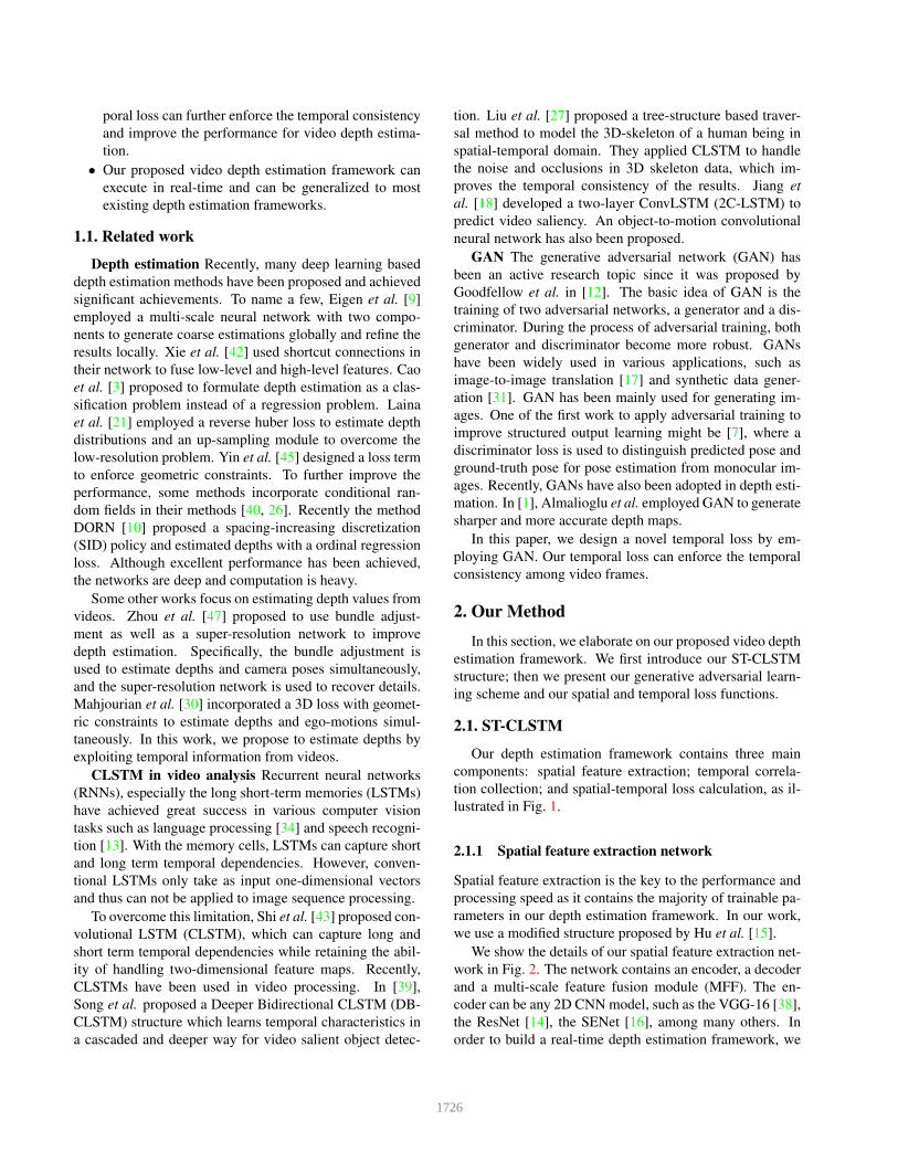
Figure 1 – Illustration of our framework. The framework contains three main parts: spatial features extraction; temporal correlations collection; and

spatial-temporal loss calculation. The first two parts consist of our ST-CLSTM structure which captures both spatial features and temporal correlations.

After the ST-CLSM generates depth estimations, a 3D CNN is introduced to calculate the temporal loss. The spatial and temporal losses are combined to

update the framework.

Frame i

Conv1 Block1 Block2 Block3 Block4

Decoder

Feature maps

Encoder

MFF

Conv2

up1x2

up2x4

up4x16

up3x8

up5x2

up6x2

up7x2

up8x2

Concatenate

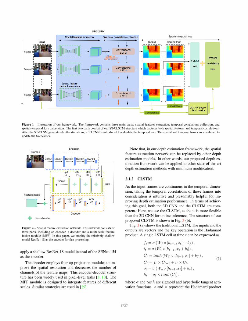
Figure 2 – Spatial feature extraction network. This network consists of

three parts, including an encoder, a decoder and a multi-scale feature

fusion module (MFF). In this paper, we employ the relatively shallow

model ResNet-18 as the encoder for fast processing.

apply a shallow ResNet-18 model instead of the SENet-154

as the encoder.

The decoder employs four up-projection modules to im-

prove the spatial resolution and decreases the number of

channels of the feature maps. This encoder-decoder struc-

ture has been widely used in pixel-level tasks [5, 10]. The

MFF module is designed to integrate features of different

scales. Similar strategies are used in [29].

Note that, in our depth estimation framework, the spatial

feature extraction network can be replaced by other depth

estimation models. In other words, our proposed depth es-

timation framework can be applied to other state-of-the-art

depth estimation methods with minimum modification.

2.1.2 CLSTM

As the input frames are continuous in the temporal dimen-

sion, taking the temporal correlations of these frames into

consideration is intuitive and presumably helpful for im-

proving depth estimation performance. In terms of achiev-

ing this goal, both the 3D CNN and the CLSTM are com-

petent. Here, we use the CLSTM, as the it is more flexible

than the 3D CNN for online inference. The structure of our

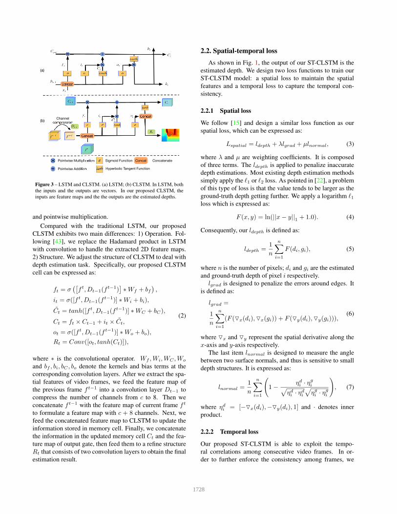
proposed CLSTM is shown in Fig. 3 (b).

Fig. 3 (a) shows the traditional LSTM. The inputs and the

outputs are vectors and the key operation is the Hadamard

product. A single LSTM cell at time t can be expressed as:

ft = σ (Wf ◦ [ht−1, xt] + bf ) ,

it = σ (Wi ◦ [ht−1, xt + bi]) ,

Ct = tanh (WC ◦ [ht−1, xt] + bC) ,

Ct = ft × Ct−1 + it × Ct,

ot = σ (Wo ◦ [ht−1, xt] + bo) ,

ht = ot × tanh (Ct) ,

(1)

where σ and tanh are sigmoid and hyperbolic tangent acti-

vation functions. ◦ and × represent the Hadamard product

1727

Pointwise Multiplication

Pointwise Addition

Concat Concatenate

Hyperbolic Tangent Function

Sigmoid Function

Concat

Concat

ConcatChannel

compression

(a)

(b)

Figure 3 – LSTM and CLSTM. (a) LSTM; (b) CLSTM. In LSTM, both

the inputs and the outputs are vectors. In our proposed CLSTM, the

inputs are feature maps and the the outputs are the estimated depths.

and pointwise multiplication.

Compared with the traditional LSTM, our proposed

CLSTM exhibits two main differences: 1) Operation. Fol-

lowing [43], we replace the Hadamard product in LSTM

with convolution to handle the extracted 2D feature maps.

2) Structure. We adjust the structure of CLSTM to deal with

depth estimation task. Specifically, our proposed CLSTM

cell can be expressed as:

ft = σ([

f t, Dt−1(ft−1)

]

∗Wf + bf)

,

it = σ([f t, Dt−1(ft−1)] ∗Wi + bi),

Ct = tanh([f t, Dt−1(ft−1)] ∗WC + bC),

Ct = ft × Ct−1 + it × Ct,

ot = σ([f t, Dt−1(ft−1)] ∗Wo + bo),

Rt = Conv([ot, tanh(Ct)]),

(2)

where ∗ is the convolutional operator. Wf ,Wi,WC ,Wo

and bf , bi, bC , bo denote the kernels and bias terms at the

corresponding convolution layers. After we extract the spa-

tial features of video frames, we feed the feature map of

the previous frame f t−1 into a convolution layer Dt−1 to

compress the number of channels from c to 8. Then we

concatenate f t−1 with the feature map of current frame f t

to formulate a feature map with c + 8 channels. Next, we

feed the concatenated feature map to CLSTM to update the

information stored in memory cell. Finally, we concatenate

the information in the updated memory cell Ct and the fea-

ture map of output gate, then feed them to a refine structure

Rt that consists of two convolution layers to obtain the final

estimation result.

2.2. Spatial­temporal loss

As shown in Fig. 1, the output of our ST-CLSTM is the

estimated depth. We design two loss functions to train our

ST-CLSTM model: a spatial loss to maintain the spatial

features and a temporal loss to capture the temporal con-

sistency.

2.2.1 Spatial loss

We follow [15] and design a similar loss function as our

spatial loss, which can be expressed as:

Lspatial = ldepth + λlgrad + µlnormal, (3)

where λ and µ are weighting coefficients. It is composed

of three terms. The ldepth is applied to penalize inaccurate

depth estimations. Most existing depth estimation methods

simply apply the ℓ1 or ℓ2 loss. As pointed in [22], a problem

of this type of loss is that the value tends to be larger as the

ground-truth depth getting further. We apply a logarithm ℓ1loss which is expressed as:

F (x, y) = ln(||x− y||1+ 1.0). (4)

Consequently, our ldepth is defined as:

ldepth =1

n

n∑

i=1

F (di, gi), (5)

where n is the number of pixels; di and gi are the estimated

and ground-truth depth of pixel i respectively.

lgrad is designed to penalize the errors around edges. It

is defined as:

lgrad =

1

n

n∑

i=1

(F (▽x(di),▽x(gi)) + F (▽y(di),▽y(gi))),(6)

where ▽x and ▽y represent the spatial derivative along the

x-axis and y-axis respectively.

The last item lnormal is designed to measure the angle

between two surface normals, and thus is sensitive to small

depth structures. It is expressed as:

lnormal =1

n

n∑

i=1

(

1−ηdi · ηgi

√

ηdi · ηdi√

ηgi · ηgi

)

, (7)

where ηdi = [−▽x(di),−▽y(di), 1] and · denotes inner

product.

2.2.2 Temporal loss

Our proposed ST-CLSTM is able to exploit the tempo-

ral correlations among consecutive video frames. In or-

der to further enforce the consistency among frames, we

1728

5x5x5 Conv 32, /2, BN+ReLU3x3x3 Max Pool, /2

5x5x5 Conv 64, /2, BN+ReLU3x3x3 Max Pool, /2

5x5x5 Conv 128, /2, BN+ReLU3x3x3 Max Pool, /2

5x5x5 Conv 256, /2, BN+ReLU3x3x3 Max Pool, /2

Global Avg Pool!"#$

RGBD 1

Binary Label

RGBD n

Figure 4 – Structure of the 3DCNN discriminator model in adversarial

learning. It contains four convolution blocks, a global average pooling

layer and a fully connected layer. It takes as input concatenated RGB-D

video frames and output a binary label which indicates the input source.

apply the generative adversarial learning scheme and de-

sign a temporal consistency loss. Specifically, after our ST-

CLSTM produces depth estimations, we introduce a three-

dimensional convolutional neural network (3D CNN) which

takes as input the estimated depth sequence and output a

score. This score represents the probability of the depth se-

quence comes from our ST-CLSTM rather than the ground-

truths. The 3D CNN is then act as a discriminator. We train

the discriminator by maximizing the probability of assign-

ing the correct label to both the estimated and ground-truth

depth sequences. Our ST-CLSTM acts as the generator. The

discriminator tries to distinguish the generator’s output (la-

belled as ‘fake’) from the ground truth depth sequence (la-

belled as ‘real’). Upon convergence we wish that the gener-

ator’s output can appear as close as possible to the ground

truth so as to confuse the discriminator. During the training

of discriminator, we train the generator simultaneously. The

objective of our generative adversarial learning is expressed

as follows:

minG

maxD

V (G,D) =

Ez∈ζ [log(D(z))] + Ex∈χ[log(1−D(G(x)))],(8)

where x = [x1, ...xn] are the input RGB frames and z =[d1, ...dn] are the ground-truth depth frames. χ and ζ are the

distributions of input RGB frames and ground-truth depths

respectively.

Since our discriminator is a binary classifier, we train it

using the cross entropy loss. The cross entropy loss then

acts as our temporal loss function. During the training of

our ST-CLSTM, we combine our temporal loss with the

aforementioned spatial loss as follows:

L = Lspatial + αLtemporal, (9)

where α is a weighting coefficient. We empirically set it to

0.1.

The detailed structure of our 3DCNN is illustrated in

Fig. 4. It is composed of 4 convolution blocks, a global av-

erage pooling layer and a fully-connected layer. Each con-

volution block contains a 3D convolution layer, followed

by a batch normalization layer, a ReLU layer and a max

pooling layer. The first 3D convolution layer and all the

max pooling layers have a stride of 2. In practice, as plot-

ted in Fig. 4, our 3DCNN takes as input concatenated RGB

and depth frames to enforce the consistency between the

video frame and the corresponding depth. In order to in-

crease the robustness of our discriminator, in our generated

input depth sequences, we randomly mix some ground-truth

depth frames with a certain probability.

Note that, the adversarial training here is mainly to en-

force temporal consistency, instead of improving the depth

accuracy of single frame’s depth as in [6].

3. Experiments

In this section, we evaluate our proposed depth estima-

tion framework on the indoor NYU Depth V2 dataset and

the outdoor KITTI dataset, and compare against a few ex-

isting depth estimation approaches.

3.1. Datasets

NYU Depth V2 contains 464 videos taken from indoor

scenes. We apply the same train/test split as in Eigen et

al. [9] which contains 249 videos for training, and 654 sam-

ples from the rest 215 videos for test. During training, we

resize the image from 640 × 480 to 320 × 240 and then

randomly crop patches of 304× 228 for training.

KITTI contains 61 outdoor video scenes captured by

cameras and depth sensors mounted on a driving car. We

apply the same train/test split as in Eigen et al. [9] which

contains 32 videos for training, and 697 samples from the

rest 29 videos for test. During training, we randomly crop

patches of size 480×320 from the original images as inputs.

3.2. Evaluation metrics

Spatial Metrics We evaluate the performance of our

framework using the commonly applied metrics defined as

follows: 1) Mean relative error (Rel): 1

N

∑N

i=1

||di−gi||1gi

; 2)

Root mean squared error (RMS):

√

1

N

∑N

i=1(di − gi)

2; 3)

Mean log10 error (log10): 1

N

∑N

i=1|| log10 di − log10 gi||1;

4) Accuracy with threshold t: Percentage of di such that

1729

max(di

gi, gidi

) = δ < t ∈ [1.25, 1.252, 1.253]. N denotes the

total number of pixels. di and gi are estimated and ground-

truth depths of pixel i, respectively.

Temporal Metrics Maintaining temporal consistency

means keeping the changes and motions among adjacent

frames of estimation results consistent with that of corre-

sponding ground truths. In order to quantitatively evaluate

the temporal consistency, we introduce two metrics: tempo-

ral change consistency (TCC) and temporal motion consis-

tency (TMC). They are defined as:

TCC(D,G) =∑n−1

i=1SSIM(abs(di − di+1), abs(gi − gi+1))

n− 1,

(10)

TMC(D,G) =∑n−1

i=1SSIM(oflow(di, di+1), oflow(gi, gi+1))

n− 1,

(11)

where D =(

d1, d2, · · · , dn)

and G =(

g1, g2, · · · , gn)

are

estimation depth maps of n consecutive frames and the cor-

responding ground truths. oflow denotes real time TV −L1

optical flow [46]. SSIM is structural similarity [41].

3.3. Implementation details

We train our proposed framework for 20 epochs. The ini-

tial learning rate of the ST-CLSTM is set to 0.0001 and de-

crease by a factor of 0.1 after every five epochs. Our spatial

feature extraction network in the ST-CLSTM is pretrained

on the ImageNet dataset. As for our 3D CNN, the initial

learning rate is set to 0.1 for the NYU Depth V2 dataset and

0.01 for the KITTI dataset. The parameters of our 3D CNN

are randomly initialized. During the generative adversarial

training, before we start to update our 3D CNN parameters,

we first train our ST-CLSTM for one epoch for the NYU

Depth V2 dataset, and two epochs for the KITTI dataset, to

make sure that our ST-CLSTM is able to generate plausible

depth estimations.

Following [15], we employ three data augmentation

methods including: 1) randomly flip the RGB image and

depth map horizontally with a probability of 50%; 2) ro-

tate the RGB image and depth map by a random degree c ∈[−5◦, 5◦]; 3) scale the brightness, contrast and saturation

values of the RGB image by a random ratio r ∈ [0.6, 1.4].

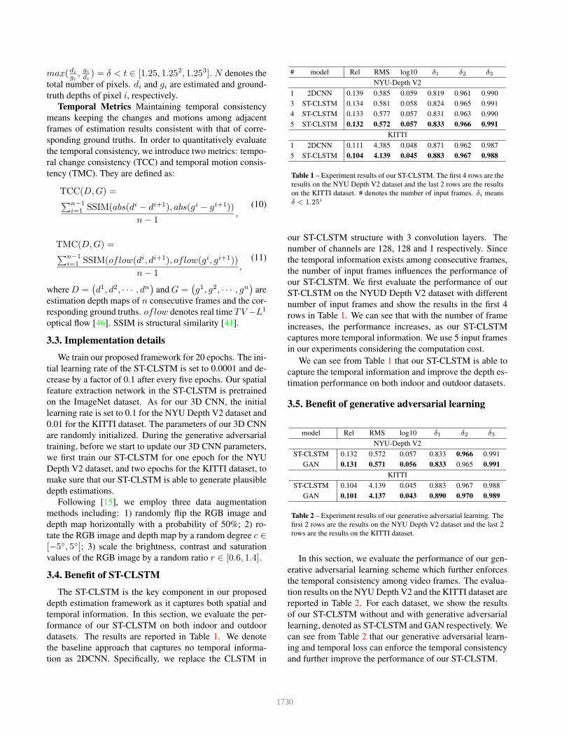
3.4. Benefit of ST­CLSTM

The ST-CLSTM is the key component in our proposed

depth estimation framework as it captures both spatial and

temporal information. In this section, we evaluate the per-

formance of our ST-CLSTM on both indoor and outdoor

datasets. The results are reported in Table 1. We denote

the baseline approach that captures no temporal informa-

tion as 2DCNN. Specifically, we replace the CLSTM in

# model Rel RMS log10 δ1 δ2 δ3

NYU-Depth V2

1 2DCNN 0.139 0.585 0.059 0.819 0.961 0.990

3 ST-CLSTM 0.134 0.581 0.058 0.824 0.965 0.991

4 ST-CLSTM 0.133 0.577 0.057 0.831 0.963 0.990

5 ST-CLSTM 0.132 0.572 0.057 0.833 0.966 0.991

KITTI

1 2DCNN 0.111 4.385 0.048 0.871 0.962 0.987

5 ST-CLSTM 0.104 4.139 0.045 0.883 0.967 0.988

Table 1 – Experiment results of our ST-CLSTM. The first 4 rows are the

results on the NYU Depth V2 dataset and the last 2 rows are the results

on the KITTI dataset. # denotes the number of input frames. δi means

δ < 1.25i

our ST-CLSTM structure with 3 convolution layers. The

number of channels are 128, 128 and 1 respectively. Since

the temporal information exists among consecutive frames,

the number of input frames influences the performance of

our ST-CLSTM. We first evaluate the performance of our

ST-CLSTM on the NYUD Depth V2 dataset with different

number of input frames and show the results in the first 4

rows in Table 1. We can see that with the number of frame

increases, the performance increases, as our ST-CLSTM

captures more temporal information. We use 5 input frames

in our experiments considering the computation cost.

We can see from Table 1 that our ST-CLSTM is able to

capture the temporal information and improve the depth es-

timation performance on both indoor and outdoor datasets.

3.5. Benefit of generative adversarial learning

model Rel RMS log10 δ1 δ2 δ3

NYU-Depth V2

ST-CLSTM 0.132 0.572 0.057 0.833 0.966 0.991

GAN 0.131 0.571 0.056 0.833 0.965 0.991

KITTI

ST-CLSTM 0.104 4.139 0.045 0.883 0.967 0.988

GAN 0.101 4.137 0.043 0.890 0.970 0.989

Table 2 – Experiment results of our generative adversarial learning. The

first 2 rows are the results on the NYU Depth V2 dataset and the last 2

rows are the results on the KITTI dataset.

In this section, we evaluate the performance of our gen-

erative adversarial learning scheme which further enforces

the temporal consistency among video frames. The evalua-

tion results on the NYU Depth V2 and the KITTI dataset are

reported in Table 2. For each dataset, we show the results

of our ST-CLSTM without and with generative adversarial

learning, denoted as ST-CLSTM and GAN respectively. We

can see from Table 2 that our generative adversarial learn-

ing and temporal loss can enforce the temporal consistency

and further improve the performance of our ST-CLSTM.

1730

Frame 1 Frame 5Frame 3 Frame 7

RGB

Ground

truth

Baseline

/2DCNN

ST-CLSTM

ST-CLSTM

+GAN

Ground

truth

Baseline

/2DCNN

ST-CLSTM

ST-CLSTM

+GAN

Figure 5 – Visual results of depth estimation on the NYU Depth V2

dataset. The top five rows are: RGB inputs, ground truth, the results of

baseline, ST-CLSTM and ST-CLSTM+GAN. For better visualization,

we present the corresponding zoom-in regions of ground truth and es-

timations results on the four bottom rows. Here, both ST-CLSTM and

ST-CLSTM+GAN are trained with 5 frames inputs. From the results

on the last row, we can see that the estimation results generated by ST-

CLSTM+GAN exhibit better temporal consistency than that of 2DCNN

and ST-CLSTM.

3.6. Improvement of temporal consistency

The major contribution of our work is to exploit tempo-

ral information for accurate depth estimation. The afore-

mentioned experiments have revealed that our proposed

ST-CLSTM and generative adversarial learning scheme are

able to better capture the temporal information and improve

the depth estimation performance. In this section, we show

the improvement of our proposed framework in the tempo-

ral dimension with both visual effects and temporal consis-

tency metrics.

We show the estimated depths of four consecutive frames

with one frame gap between each frame in Fig. 5. We first

show the RGB frames and the ground-truth depth maps in

the first two rows, then we show the depth estimations of the

baseline method (2DCNN) and our proposed framework in

Model Rel RMS log10 δ1 δ2 δ3 TCC TMC

Baseline 0.139 0.585 0.059 0.819 0.961 0.990 0.846 0.956

ST-CLSTM 0.132 0.572 0.057 0.833 0.966 0.991 0.866 0.962

3D-GAN 0.131 0.571 0.056 0.833 0.965 0.991 0.870 0.965

Table 3 – Experiment results on NYU Depth V2.

the last three rows.

We highlight a front area and a background area in

blue and red dotted windows respectively, and we maxi-

mize the blue dotted window for better visualization. Since

the four frames are consecutive, the ground-truth depths in

these four frames change smoothly. However, the baseline

method fails to maintain the smoothness. The estimated

depths vary largely. Our ST-CLSTM captures the tempo-

ral correlations and produces visually better performance

as demonstrated in Fig. 5. For all the frames, the edges

of objects are sharper and the backgrounds are smoother.

With our proposed generative adversarial learning scheme,

the temporal consistency is enforced and the performance is

further improved. The details are well maintained in all the

frames. For instance, the bars of the chair in the red dotted

window.1

3D CNN can capture the change and motion information

between consecutive frames, as it convolves the input along

both the spatial and temporal dimensions. To confuse the

3D CNN discriminator, the change and motion of estima-

tion results must keep consistent with that of corresponding

ground truths. We sampled 654 sequences from test set with

a length of 16 frames each and report the average TCC and

TMC in Table 3, from which we can see that the 3D CNN

discriminator does not only improve the estimation accu-

racy, but also better enforces the temporal consistency.

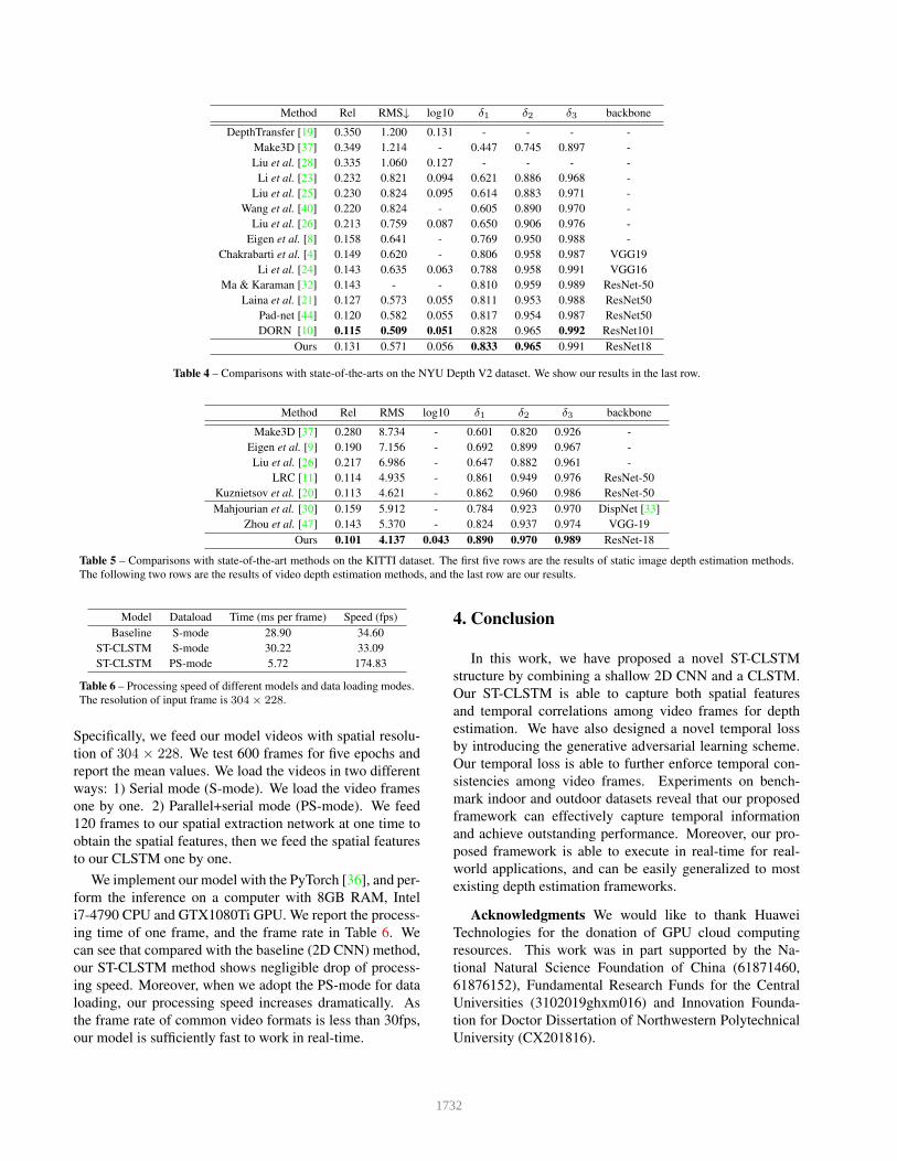
3.7. Comparisons with state­of­the­art results

In this section, we evaluate our approach on the NYU

Depth V2 dataset and the KITTI dataset and compare with

some state-of-the-art results. The results are reported in Ta-

ble 4 and Table 5 respectively. We can see that with our

captured temporal information, we outperform most state-

of-the-art methods which often use more complicated net-

work structures. The aim of our work is to exploit temporal

information for real-time depth estimation. We apply a shal-

low ResNet18 model as our backbone. The performance of

our approach can be improved with deeper backbone net-

works. We leave this as future work.

3.8. Speed analysis

One of the contributions of our work here is that our

model can execute in real-time for practical applications. In

this section, we evaluate the processing time of our model.

1Readers may refer to the demonstration video: https://youtu.

be/B705k8nunLU

1731

Method Rel RMS↓ log10 δ1 δ2 δ3 backbone

DepthTransfer [19] 0.350 1.200 0.131 - - - -

Make3D [37] 0.349 1.214 - 0.447 0.745 0.897 -

Liu et al. [28] 0.335 1.060 0.127 - - - -

Li et al. [23] 0.232 0.821 0.094 0.621 0.886 0.968 -

Liu et al. [25] 0.230 0.824 0.095 0.614 0.883 0.971 -

Wang et al. [40] 0.220 0.824 - 0.605 0.890 0.970 -

Liu et al. [26] 0.213 0.759 0.087 0.650 0.906 0.976 -

Eigen et al. [8] 0.158 0.641 - 0.769 0.950 0.988 -

Chakrabarti et al. [4] 0.149 0.620 - 0.806 0.958 0.987 VGG19

Li et al. [24] 0.143 0.635 0.063 0.788 0.958 0.991 VGG16

Ma & Karaman [32] 0.143 - - 0.810 0.959 0.989 ResNet-50

Laina et al. [21] 0.127 0.573 0.055 0.811 0.953 0.988 ResNet50

Pad-net [44] 0.120 0.582 0.055 0.817 0.954 0.987 ResNet50

DORN [10] 0.115 0.509 0.051 0.828 0.965 0.992 ResNet101

Ours 0.131 0.571 0.056 0.833 0.965 0.991 ResNet18

Table 4 – Comparisons with state-of-the-arts on the NYU Depth V2 dataset. We show our results in the last row.

Method Rel RMS log10 δ1 δ2 δ3 backbone

Make3D [37] 0.280 8.734 - 0.601 0.820 0.926 -

Eigen et al. [9] 0.190 7.156 - 0.692 0.899 0.967 -

Liu et al. [26] 0.217 6.986 - 0.647 0.882 0.961 -

LRC [11] 0.114 4.935 - 0.861 0.949 0.976 ResNet-50

Kuznietsov et al. [20] 0.113 4.621 - 0.862 0.960 0.986 ResNet-50

Mahjourian et al. [30] 0.159 5.912 - 0.784 0.923 0.970 DispNet [33]

Zhou et al. [47] 0.143 5.370 - 0.824 0.937 0.974 VGG-19

Ours 0.101 4.137 0.043 0.890 0.970 0.989 ResNet-18

Table 5 – Comparisons with state-of-the-art methods on the KITTI dataset. The first five rows are the results of static image depth estimation methods.

The following two rows are the results of video depth estimation methods, and the last row are our results.

Model Dataload Time (ms per frame) Speed (fps)

Baseline S-mode 28.90 34.60

ST-CLSTM S-mode 30.22 33.09

ST-CLSTM PS-mode 5.72 174.83

Table 6 – Processing speed of different models and data loading modes.

The resolution of input frame is 304× 228.

Specifically, we feed our model videos with spatial resolu-

tion of 304 × 228. We test 600 frames for five epochs and

report the mean values. We load the videos in two different

ways: 1) Serial mode (S-mode). We load the video frames

one by one. 2) Parallel+serial mode (PS-mode). We feed

120 frames to our spatial extraction network at one time to

obtain the spatial features, then we feed the spatial features

to our CLSTM one by one.

We implement our model with the PyTorch [36], and per-

form the inference on a computer with 8GB RAM, Intel

i7-4790 CPU and GTX1080Ti GPU. We report the process-

ing time of one frame, and the frame rate in Table 6. We

can see that compared with the baseline (2D CNN) method,

our ST-CLSTM method shows negligible drop of process-

ing speed. Moreover, when we adopt the PS-mode for data

loading, our processing speed increases dramatically. As

the frame rate of common video formats is less than 30fps,

our model is sufficiently fast to work in real-time.

4. Conclusion

In this work, we have proposed a novel ST-CLSTM

structure by combining a shallow 2D CNN and a CLSTM.

Our ST-CLSTM is able to capture both spatial features

and temporal correlations among video frames for depth

estimation. We have also designed a novel temporal loss

by introducing the generative adversarial learning scheme.

Our temporal loss is able to further enforce temporal con-

sistencies among video frames. Experiments on bench-

mark indoor and outdoor datasets reveal that our proposed

framework can effectively capture temporal information

and achieve outstanding performance. Moreover, our pro-

posed framework is able to execute in real-time for real-

world applications, and can be easily generalized to most

existing depth estimation frameworks.

Acknowledgments We would like to thank Huawei

Technologies for the donation of GPU cloud computing

resources. This work was in part supported by the Na-

tional Natural Science Foundation of China (61871460,

61876152), Fundamental Research Funds for the Central

Universities (3102019ghxm016) and Innovation Founda-

tion for Doctor Dissertation of Northwestern Polytechnical

University (CX201816).

1732

References

[1] Yasin Almalioglu, Muhamad Risqi Saputra, Pedro de Gus-

mao, Andrew Markham, and Niki Trigoni. GANVO: Unsu-

pervised deep monocular visual odometry and depth estima-

tion with generative adversarial networks. In Proc. IEEE Int.

Conf. Robotics Automation., 2019. 2

[2] Guido Borghi, Marco Venturelli, Roberto Vezzani, and Rita

Cucchiara. Poseidon: Face-from-depth for driver pose esti-

mation. In Proc. IEEE Conf. Comp. Vis. Patt. Recogn., pages

4661–4670, 2017. 1

[3] Yuanzhouhan Cao, Zifeng Wu, and Chunhua Shen. Esti-

mating depth from monocular images as classification using

deep fully convolutional residual networks. IEEE Trans. Cir-

cuits Syst. Video Technol., 28:3174–3182, 2018. 2

[4] Ayan Chakrabarti, Jingyu Shao, and Greg Shakhnarovich.

Depth from a single image by harmonizing overcomplete lo-

cal network predictions. In Proc. Advances in Neural Inf.

Process. Syst., pages 2658–2666, 2016. 8

[5] Liang-Chieh Chen, Yukun Zhu, George Papandreou, Florian

Schroff, and Hartwig Adam. Encoder-decoder with atrous

separable convolution for semantic image segmentation. In

Proc. Eur. Conf. Comp. Vis., pages 801–818, 2018. 3

[6] Richard Chen, Faisal Mahmood, Alan Yuille, and Nicholas J.

Durr. Rethinking monocular depth estimation with adversar-

ial training. arXiv: Comp. Res. Repository, 2018. 5

[7] Yu Chen, Chunhua Shen, Xiu-Shen Wei, Lingqiao Liu, and

Jian Yang. Adversarial PoseNet: A structure-aware convo-

lutional network for human pose estimation. In Proc. IEEE

Int. Conf. Comp. Vis., 2017. 2

[8] David Eigen and Rob Fergus. Predicting depth, surface nor-

mals and semantic labels with a common multi-scale convo-

lutional architecture. In Proc. IEEE Int. Conf. Comp. Vis.,

pages 2650–2658, 2015. 8

[9] David Eigen, Christian Puhrsch, and Rob Fergus. Depth map

prediction from a single image using a multi-scale deep net-

work. In Proc. Advances in Neural Inf. Process. Syst., pages

2366–2374, 2014. 1, 2, 5, 8

[10] Huan Fu, Mingming Gong, Chaohui Wang, Kayhan Bat-

manghelich, and Dacheng Tao. Deep ordinal regression net-

work for monocular depth estimation. In Proc. IEEE Conf.

Comp. Vis. Patt. Recogn., pages 2002–2011, 2018. 1, 2, 3, 8

[11] Clément Godard, Oisin Mac Aodha, and Gabriel Brostow.

Unsupervised monocular depth estimation with left-right

consistency. In Proc. IEEE Conf. Comp. Vis. Patt. Recogn.,

pages 270–279, 2017. 8

[12] Ian Goodfellow, Jean Pouget-Abadie, Mehdi Mirza, Bing

Xu, David Warde-Farley, Sherjil Ozair, Aaron Courville, and

Yoshua Bengio. Generative adversarial nets. In Proc. Ad-

vances in Neural Inf. Process. Syst., pages 2672–2680, 2014.

2

[13] Alex Graves, Abdel-rahman Mohamed, and Geoffrey Hin-

ton. Speech recognition with deep recurrent neural networks.

In Proc. IEEE Int. Conf. Acoust. Speech Signal Process.,

pages 6645–6649. IEEE, 2013. 2

[14] Kaiming He, Xiangyu Zhang, Shaoqing Ren, and Jian Sun.

Deep residual learning for image recognition. In Proc. IEEE

Conf. Comp. Vis. Patt. Recogn., pages 770–778, 2016. 2

[15] Junjie Hu, Mete Ozay, Yan Zhang, and Takayuki Okatani.

Revisiting single image depth estimation: toward higher res-

olution maps with accurate object boundaries. In IEEE Win-

ter Conf. Appl. Comp. Vis., pages 1043–1051. IEEE, 2019.

2, 4, 6

[16] Jie Hu, Li Shen, and Gang Sun. Squeeze-and-excitation net-

works. In Proc. IEEE Conf. Comp. Vis. Patt. Recogn., pages

7132–7141, 2018. 2

[17] Phillip Isola, Jun-Yan Zhu, Tinghui Zhou, and Alexei A

Efros. Image-to-image translation with conditional adversar-

ial networks. In Proc. IEEE Conf. Comp. Vis. Patt. Recogn.,

pages 1125–1134, 2017. 2

[18] Lai Jiang, Mai Xu, and Zulin Wang. Predicting video

saliency with object-to-motion cnn and two-layer convolu-

tional lstm. arXiv: Comp. Res. Repository, abs/1709.06316,

2017. 2

[19] Kevin Karsch, Ce Liu, and Sing Bing Kang. Depth transfer:

Depth extraction from video using non-parametric sampling.

IEEE Trans. Pattern Anal. Mach. Intell., 36(11):2144–2158,

2014. 8

[20] Yevhen Kuznietsov, Jorg Stuckler, and Bastian Leibe. Semi-

supervised deep learning for monocular depth map predic-

tion. In Proc. IEEE Conf. Comp. Vis. Patt. Recogn., pages

6647–6655, 2017. 8

[21] Iro Laina, Christian Rupprecht, Vasileios Belagiannis, Fed-

erico Tombari, and Nassir Navab. Deeper depth prediction

with fully convolutional residual networks. In International

conference on 3D vision, pages 239–248. IEEE, 2016. 1, 2,

8

[22] Jae-Han Lee, Minhyeok Heo, Kyung-Rae Kim, and Chang-

Su Kim. Single-image depth estimation based on fourier do-

main analysis. In Proc. IEEE Conf. Comp. Vis. Patt. Recogn.,

2018. 4

[23] Bo Li, Chunhua Shen, Yuchao Dai, Anton Van Den Hen-

gel, and Mingyi He. Depth and surface normal estimation

from monocular images using regression on deep features

and hierarchical crfs. In Proc. IEEE Conf. Comp. Vis. Patt.

Recogn., pages 1119–1127, 2015. 8

[24] Jun Li, Reinhard Klein, and Angela Yao. A two-streamed

network for estimating fine-scaled depth maps from single

RGB images. In Proc. IEEE Int. Conf. Comp. Vis., pages

3372–3380, 2017. 8

[25] Fayao Liu, Chunhua Shen, and Guosheng Lin. Deep con-

volutional neural fields for depth estimation from a single

image. In Proc. IEEE Conf. Comp. Vis. Patt. Recogn., pages

5162–5170, 2015. 8

[26] Fayao Liu, Chunhua Shen, Guosheng Lin, and Ian Reid.

Learning depth from single monocular images using deep

convolutional neural fields. IEEE Trans. Pattern Anal. Mach.

Intell., 38(10):2024–2039, 2016. 2, 8

[27] Jun Liu, Amir Shahroudy, Dong Xu, and Gang Wang.

Spatio-temporal lstm with trust gates for 3d human action

recognition. In Proc. Eur. Conf. Comp. Vis., pages 816–833.

Springer, 2016. 2

[28] Miaomiao Liu, Mathieu Salzmann, and Xuming He.

Discrete-continuous depth estimation from a single image.

In Proc. IEEE Conf. Comp. Vis. Patt. Recogn., pages 716–

723, 2014. 8

1733

[29] Jonathan Long, Evan Shelhamer, and Trevor Darrell. Fully

convolutional networks for semantic segmentation. In Proc.

IEEE Conf. Comp. Vis. Patt. Recogn., pages 3431–3440,

2015. 3

[30] Reza Mahjourian, Martin Wicke, and Anelia Angelova. Un-

supervised learning of depth and ego-motion from monoc-

ular video using 3d geometric constraints. In Proc. IEEE

Conf. Comp. Vis. Patt. Recogn., pages 5667–5675, 2018. 1,

2, 8

[31] Faisal Mahmood, Richard Chen, and Nicholas J Durr. Un-

supervised reverse domain adaptation for synthetic medical

images via adversarial training. IEEE Trans. Med. Imaging,

37(12):2572–2581, 2018. 2

[32] Fangchang Mal and Sertac Karaman. Sparse-to-dense:

Depth prediction from sparse depth samples and a single im-

age. In Proc. IEEE Int. Conf. Robotics Automation., pages

1–8. IEEE, 2018. 8

[33] Nikolaus Mayer, Eddy Ilg, Philip Hausser, Philipp Fischer,

Daniel Cremers, Alexey Dosovitskiy, and Thomas Brox. A

large dataset to train convolutional networks for disparity,

optical flow, and scene flow estimation. In Proc. IEEE Conf.

Comp. Vis. Patt. Recogn., pages 4040–4048, 2016. 8

[34] Tomáš Mikolov, Stefan Kombrink, Lukáš Burget, Jan Cer-

nocky, and Sanjeev Khudanpur. Extensions of recurrent neu-

ral network language model. In Proc. IEEE Int. Conf. Acoust.

Speech Signal Process., pages 5528–5531. IEEE, 2011. 2

[35] Piotr Mirowski, Razvan Pascanu, Fabio Viola, Hubert Soyer,

Andrew J Ballard, Andrea Banino, Misha Denil, Ross

Goroshin, Laurent Sifre, Koray Kavukcuoglu, et al. Learn-

ing to navigate in complex environments. arXiv: Comp. Res.

Repository, abs/1611.03673, 2016. 1

[36] Adam Paszke, Sam Gross, Soumith Chintala, Gregory

Chanan, Edward Yang, Zachary DeVito, Zeming Lin, Al-

ban Desmaison, Luca Antiga, and Adam Lerer. Automatic

differentiation in pytorch. 2017. 8

[37] Ashutosh Saxena, Min Sun, and Andrew Y Ng. Make3d:

Learning 3d scene structure from a single still image. IEEE

Trans. Pattern Anal. Mach. Intell., 31(5):824–840, 2009. 8

[38] Karen Simonyan and Andrew Zisserman. Very deep convo-

lutional networks for large-scale image recognition. arXiv:

Comp. Res. Repository, abs/1409.1556, 2014. 2

[39] Hongmei Song, Wenguan Wang, Sanyuan Zhao, Jianbing

Shen, and Kin-Man Lam. Pyramid dilated deeper convlstm

for video salient object detection. In Proc. Eur. Conf. Comp.

Vis., pages 715–731, 2018. 2

[40] Peng Wang, Xiaohui Shen, Zhe Lin, Scott Cohen, Brian

Price, and Alan L Yuille. Towards unified depth and semantic

prediction from a single image. In Proc. IEEE Conf. Comp.

Vis. Patt. Recogn., pages 2800–2809, 2015. 2, 8

[41] Zhou Wang, Alan Bovik, Hamid Sheikh, and Eero Simon-

celli. Image quality assessment: from error visibility to struc-

tural similarity. IEEE Trans. Image Process., 13(4):600–612,

2004. 6

[42] Junyuan Xie, Ross Girshick, and Ali Farhadi. Deep3d:

Fully automatic 2d-to-3d video conversion with deep con-

volutional neural networks. In Proc. Eur. Conf. Comp. Vis.,

pages 842–857. Springer, 2016. 2

[43] Shi Xingjian, Zhourong Chen, Hao Wang, Dit-Yan Yeung,

Wai-Kin Wong, and Wang-chun Woo. Convolutional lstm

network: A machine learning approach for precipitation

nowcasting. In Proc. Advances in Neural Inf. Process. Syst.,

pages 802–810, 2015. 2, 4

[44] Dan Xu, Wanli Ouyang, Xiaogang Wang, and Nicu Sebe.

Pad-net: multi-tasks guided prediction-and-distillation net-

work for simultaneous depth estimation and scene parsing.

In Proc. IEEE Conf. Comp. Vis. Patt. Recogn., pages 675–

684, 2018. 8

[45] Wei Yin, Yifan Liu, Chunhua Shen, and Youliang Yan. En-

forcing geometric constraints of virtual normal for depth pre-

diction. In Proc. IEEE Int. Conf. Comp. Vis., 2019. 2

[46] Christopher Zach, Thomas Pock, and Horst Bischof. A du-

ality based approach for realtime tv-l 1 optical flow. In Proc.

Annual Symp. German Assoc. Pattern Recogn., pages 214–

223. Springer, 2007. 6

[47] Lipu Zhou, Jiamin Ye, Montiel Abello, Shengze Wang, and

Michael Kaess. Unsupervised learning of monocular depth

estimation with bundle adjustment, super-resolution and clip

loss. arXiv: Comp. Res. Repository, abs/1812.03368, 2018.

1, 2, 8

1734