ANNALS OF PHYSICS: 51, 187-200 (1969)

Explicit Solution of the Continuous Baker-Campbell-Hausdorff Problem and a New Expression for the Phase Operator

I. BIALYNICKI-BIRULA, B. MIELNIK, AND J. PLEBA~~SKI

Institute of Theoretical Physics, Warsaw University, Warsaw, Poland

An explicit formula for an arbitrary function of the evolution operator is derived. With its use, the continuous analog of the Baker-Campbell-Hausdorff problem is solved. The application of this result to the quantum theory of scattering leads to a new closed expression for the phase shifts in every order of perturbation theory.

I. INTRODUCTION

In many branches of physics and mathematics we are led to study the evolution equation

(1.1)

The purpose of this paper is the derivation of a new representation for an arbitrary function of E, the evolution 0perator.l Using this representation for the function Sz = In E, we obtain the solution of the continuous analog of the Baker-Campbell-Hausdorff problem (I), (2) in a closed form.

We discuss also briefly in this paper one of the most interesting applications of our result, namely, to the scattering theory in quantum mechanics, and we derive an explicit formula for the phase shifts in every order of perturbation theory.

The evolution equation (1.1) and the initial condition for the evolution operator,

J%l 9 44 = 1, (1.2)

are equivalent to the following integral equation

1 We shall call traditionally all objects like A(t), E(r, &,) etc. the operators even though they need not be defined as operators in a vector space. All we shall need is that they form an asso- ciative algebra.

187

188 BIALYNICKI-BIRULA, MIELNIK, AND PLEBAfiSKI

The formal iterative solution2 of this equation has the form

where

The infinite series (1.4) is often written in the form of Dyson’s time-ordered exponential (3)

W, to) = T ew (/la 4 4t3). (1.6)

This representation of the evolution operator has been successfully used in quantum theories, especially in quantum electrodynamics, to obtain approximate expressions for the transition amplitudes.

The exponential representation (1.6) of the evolution operator is generalized in this paper to an arbitrary functionf(E - 1) of the evolution operator. Assuming, without any real loss of generality, thatf(0) = 1, we derive the following formula forf(E - I),

f@ - 1) = Fexp (j:, 4 A(G),

where the ordering operation F depends on the function f and is a generalization of the time-ordering of Dyson.

In Section II we derive, with the use of a resolvent operator, a simple closed formula for f(E - l), called by us the canonical representation. This canonical representation serves as an intermediate step in the derivation of (1.7), but has also some direct applications.

In Section III we introduce the concept of the F-ordering operation and we transform the canonical representation to the form (1.7). We study also in some detail the ordering operation L connected with the logarithm of the evolution operator.

In Section IV we apply our formulae for the logarithm of the evolution operator to the quantum theory of scattering. We discuss some advantages of using this

a Problems of existence and covergence will not be investigated here. The formulae appearing in this paper should be understood as purely algebraic relations in the spirit of formal power series approach.

CONTINUOUS BAKER-HAUSDORFF FORMULA 189

new representation for the phase operator in the scattering theory and we derive an explicit integral formula for the phase shift in every order of perturbation theory.

We restrict ourselves in this paper to an application in the scattering theory, but we think that our results can be also applied in other fields of physics and mathematics. To give just a few examples we may mention here possible applica- tions to statistical physics (the Liouville equation, the master equation, the Bloch equation, the Boltzmann equation), to group theory (construction of group elements from generators) and to systems of ordinary differential equations.

II. THE CANONICAL REPRESENTATION

We show in this section, that every function f of the evolution operator, which is analytic at z = 0, can be represented in the following canonical form

and

0, = o,(t, ,..., td = knwl + en-l,n--2 + - + 4,. (2.3)

Function 0, takes on values 0, l,..., II - 1 and we set 0, = 0 consistently. The canonical form off(T) is most easily found with the use of the resolvent

operator R,

where h is a complex parameter and

Ekl = E(tk - tL) = 2e(t, - tl) - 1. (2.5)

The resolvent operator R reduces to T when x is set equal to 1.

R(t, to ; A)[,=, = +T(t, to). (2.6)

3 We shall drop the index n and write 0, instead of 8,) whenever it will not lead to a confusion.

190 BIALYNICKI-BIRULA, MIELNIK, AND PLEBAtiSKI

The resolvent operator can be brought to the canonical form with the use of the following identity

; (%.,-1 + a *** ($1 + A) = & (A + l)@ (h - I)“-e-1. (2.7)

The operator R obeys the following simple differential equation.

; R(t, to ; h) = R2(r, t,, ; h). w9

TO prove this we write R in a symbolic form,

Using the dot to denote the product of two operators, which contain independent integrations with respect to tn . . . tI, and tkwl . . . tl , we can write

+~jA(E+X)A(E+X)A.~jA+..‘. (2.10)

The right-hand side in this equation is easily seen to be the formal product of two series (2.9).

The explicit solution of Eq. (2.8) is

R(t, to ; h) = %(tP to) 1 - AR&, to) ’

(2.11)

where

Rdt, to) = R(t, t,, ; AL, . (2.12)

It follows from (2.1 I), that all powers of R can be expressed in terms of its derivatives

Rn+l - 1 a”R - n! ahn’

(2.13)

Some additional properties of R are discussed in the Appendix.

CONTINUOUS BAKER-HAUSDORFF FORMULA 191

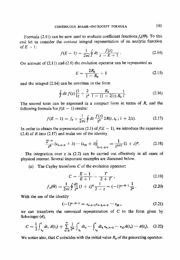
Formula (2.11) can be now used to evaluate coefficient functions&(@). To this end let us consider the contour integral representation of an analytic function OfE- 1:

On account of (2.11) and (2.6) the evolution operator can be represented as

and the integral (2.14) can be rewritten in the form

(2.14)

(2.16)

The second term can be expressed in a compact form in terms of R, and the following formula for f(E - 1) results:

f (E - 1) = f, + & f dz 9 2R(t, t,, ; 1 + 2/z). (2.17)

In order to obtain the representation (2.1) off(E - I), we introduce the expansion (2.4) of R into (2.17) and make use of the identity

~(%~-l + 4 +*- cc21 + qh 1+2,2 = A(1 + z)? (2.18)

The integration over z in (2.2) can be carried out effectively in all cases of physical interest. Several important examples are discussed below.

(a) The Cayley transform C of the evolution operator:

c= E---l T -=-> E-l-1 2-l-T

f@) = & $ g (1 + z)” & = (-1)+-B--l &.

(2.19)

(2.20)

With the use of the identity

(-l)n-e-1 = E,,,-1E,-1,12-2 *** E21, (2.21)

we can transform the canonical representation of C to the form given by Schwinger (4),

C = ; s:, dt, A(h) + nt2& s:, dt, *-- s” dtl c,z,sl ... c21A(t,J ... A&). (2.22) to

We notice also, that C coincides with the initial value R, of the generating operator.

192 BIALYNICKI-BIRULA, MIELNIK, AND PLEBAIbKI

(b) Arbitrary power ED of the evolution operator (JJ may be real or complex):

Ep = (1 + T)“, (2.23)

(1 + zY+,’ = ; (0 + p)(O + p - 1) **a (0 + p - n + 1), (2.24)

ED = 1 + nzl $ i:, dt, .*a it dt,(O + p) *.* (0 + p - n - 1) A@,) -*- A&). to (2.25)

Known expansions for E and E-l are obtained from (2.26) with the use of the identities

$(@ + 1) *-- (0 - 12 + 2) = BQ& = 8,& *** e,, , (2.26)

$0 - 1) ‘.. (0 - n) = (-l)n ss,O = (-l)n e,, a** 8,-r,, . (2.27)

(c) The logarithm Q of the evolution operator:

E = eR, D = ln(1 + T), (2.28)

m=&+l (1 + z)@ In(1 + z) = (-l>n-@-I $ O!(n - 0 - l)!. (2.29)

The canonical representation of 1;2 has the form

Q = $$ j:odh *-* jt dt,(--l)+@-l @!(n - 0 - I)! A(t,J .a. A@,). (2.30) to

In the next section we study the properties of 52 in some detail.

III. F-ORDERING OPERATIONS

Since only the symmetric part of the integrand contributes to the n-fold integral, we can rewrite the canonical representation (2.1) of f(E - 1) in the following symmetrized form,

f(E - 1) = h + fjl; f/n -*- f.dt, F(A(t,J ..a A(Q), (3.1)

(3.2)

CONTINUOUS BAKER-HAUSDORFF FORMULA 193

and the sum is extended over all n ! permutations rr of the indices in ,..., il . We call FtAn ... A,) the F-ordered product of operators A, ,..., A, . The simplest examples of F-ordered products are well known T-ordered (chronological) and Bordered (antichronological) products.

With the use of the same convention, that is adopted for the T-ordered products, namely, that the ordering operation is to be performed before the integrations, we can write (3.1) in the form

f(E - 1) = h - 1 + Few (j:,dh A(h)). (3.3)

This formula reduces to (1.7) when, as we had assumed before,f, = 1. Due to the symmetry of F(A(t,J *.a A(Q) with respect to tn ,..., t, , we can

reduce every integration in (3.1) to the integration over the simplex defined by the inequalities

t, > tnel > *** > t, ; (3.4)

f(E - 1) = So + nfl jio dt, *** j;;h Ft.Wn> a-* Aft,)). (3.5)

When the conditions (3.4) are satisfied, @(t. %, ,..., tc,) in (3.2) becomes a function of the permutation rr only. We shall denote this function by O(r). Its value is equal to the total number of chronologically ordered neighbors (i.e., tik > ti,-,) in the permutation rr,

@(?T) = @(fin )..., ti,) tn > tn-1 > *-’ t, . (3.6)

We devote the rest of this section to the study of one important ordering operation: that for the logarithm of E. We call the expression (3.2) in this case the L-ordered product and we can express it for t, > *** > t, in the form

L(A(tJ a-. A(&)) = $ c (-l)+@(“-l [e(r)]! [n - @(z-) - l]! A(&,) -.. A(ti,). * n (3.7)

For n = 1, 2, 3, 4, 5 we obtain

(3.8a)

(3.8b)

(3.8~)

(3.8d)

595/51/I-13

194 BIALYNICKI-BIRULA, MIELNIK, AND PLEBArjSKI

+ %42A*A.¶A5A,l + ~A,AlA3A,A4~ + bGbu2A31 + ~~44,&444 + 2{A,A4A,A,A,l + 3{AIA,A,A,A,l)>

where Ai = A(&) and i } denotes the multiple commutator,

(3.8e)

MA-, *.- 4 = [A,,, [An-1 ,..., [A,, 41 -**Il. (3.9)

Integrating L(A(tJ *a* A@,)) according to the formula (3.5) we obtain the nth order term in the expansion of Q. Lower order terms of this expansion have been calculated in the literature before by iterative methods. Recently, Wilcox (5) carried out this calculation up to n = 4.

It can be generally proved, that in every order of perturbation theory D is a linear combination of integrated multiple commutators. This follows either from the Friedrichs theorem (2) or more directly from the differential equation (A.7) for Q derived in the Appendix of this paper. Knowing this multiple commutator structure of 52, we can transform the r.h.s. in (3.7), with the use of the Dynkin- Specht-Weaver theorem (2), to the form

L(A(t,) a.. A@,)) = ; c (- 1) R - e(n)-1 * R

[63(n)]! [n - S(r) - l]! ; {A(&> *** A(&J}.

(W

It is actually this form of L that we used to evaluate formulae (3.8).

IV. PHASE OPERATOR AND PHASE SHIFTS

In this section we apply our results to the quantum scattering theory and we derive an explicit integral expression for the phase shift in an arbitrary order of perturbation theory. Our representation of the logarithm of the evolution operator is expected to be especially useful in this case since all approximate expressions for the phase operator obtained in perturbation theory would lead to unitary evolution operators. No violation of unitarity, often found in ordinary perturbation theory will appear in this method.

For simplicity, we restrict ourselves in this paper to the nonrelativistic quantum mechanics. Applications to relativistic quantum mechanics and field theory will be presented in a separate publication.

CONTINUOUS BAKER-HAUSDORFF FORMULA 195

Let us consider scattering of a particle with the mass p by the static potential I’. The unitary evolution operator U(t, t) in the Dirac representation obeys the equation

$ U(t, to) = -iVdt) WC &I>, (4.1)

where J/,(t) = pot T/e-“w (4.2)

and Ho = @12/A. (4.3)

With the use of the canonical representation (2.1) we can express any function f of the S operator, S = U(co, - co), in the form

X (1 + ze,,,-,) ... (1 + zf&) eiHotnVe-i*o’t”-tn-l’V *a* VemiHo’l. (4.4)

In the formula for the matrix element of f(S - l), in any representation in which H,, is diagonal, all ti integrations can be carried out leaving us with the following formula

(E’, 01’ I (f (S - 1) - fo> I E, a>

= 6(E - E’) f (-1)” $ d[ f(l/LJ(E’, a’ I VG,(E)V a*. VG,(E)V I E, a> 9Z=l

= --SW - E') f 4fU/W', a' I W + G,(E)V)-l I E, a>,

where

G,(E) = P H 0

(4.5)

and the integration in the <-plane is to be carried out along the closed contour obtained by the inversion: 5 = l/z from the contour defined before in the complex z-plane.

In the simplest case of a spherically symmetric potential we can use the complete set of spherical waves to derive an explicit integral formula for the matrix element (4.5).

We introduce the following notation

VdE, E’) = <E, 1, m I V I E’, I, m>, (4.7)

g,(E - E’) = P & + im(l + 25) S(E - E’), (4.8)

196 BIALYNICKI-BIRULA, MIELNIK, AND PLEBArjSKI

and use the completeness and orthonormality of the set 1 E, I, m),

~~~IE,I,m)dE(E,I,m/ = 1,

(E, I, m 1 E’, I’, ml> = S,,J,,4(E - E’)

and the relations

(4.9a)

(4.9b)

V 1 E, I, m> = SW dE’ V,(E, E’) 1 E’, I, m>, 0

(4.10)

G,tE’) I E, 6 m> = gdE - E’) I E, 4 m>. (4.11)

Wavefunctions (x 1 E, 1, m) are well known spherical waves

<x I E, 4 m> = (+)l” Jl+l12tkr) Y,“(y, 4, (4.12)

where k = (2t~E)‘/~, (4.13)

so that the reduced matrix element V,(E, E’) can be expressed as an integral of V(r) and Bessel functions,

VdE, E’) = P jm dr rJz+,,,tkr) V(r) J~+112Wr)- (4.14) 0

With the help of Eqs. (4.7)-(4.11), we can transform the expression (4.5) to the form

<E’, I’, m’ I (W - 1) - .A,) I 4 6 m>

= 6,,&,4(E - E’) 2 (-1)” $ d5 f(1/5) j-y dE, *.. j.; dEnml V&=1

* V,tE, El) gc& - E) VdE2 , Ed *** gd&-1 - E> VdL-1 , E). (4.15)

The following integral relation between Bessel and Neumann functions (6)

gdr, r’; E, 0 ; s * dE, Jt+l,2tk,r) g& - 9 J~+&~r’~ 0

= - +Kr - r’> JJl+l,2(kr) Jl+&r’) + 4r’ - r) J~+dkr) ~~+dW

- W + 25) J1+1,2W) Jr+I,2W)l (4.16)

enables us to express every term in (4.15) as an integral over 5 and r, ,..., r,, only.

CONTINUOUS BAKER-HAUSDORFF FORMULA 197

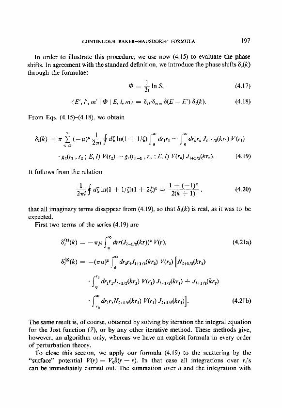
In order to illustrate this procedure, we use now (4.15) to evaluate the phase shifts. In agreement with the standard definition, we introduce the phase shifts &(k) through the formulae:

@ = 4 In S, (4.17)

(E’, I’, m’ 1 Q, 1 E, Z, mj = 6,,4,,%3(E - E’) 6,(k). (4.18)

From Eqs. (4.15)-(4.18) we obtain

. gdr, , r2 ; E, 0 VP,> ..* g&n-l , rn ; E, 0 W-d J~+l,2(krn). (4.19)

It follows from the relation

(4.20)

that all imaginary terms disappear from (4.19) so that 6,(k) is real, as it was to be expected.

First two terms of the series (4.19) are

6i1’(k) = -np jm drr(Jz+,,,(kr))2 V(r), 0

(4.21a)

@“‘W = 4~)~ jm dr2r2Jz+l,2(kr2) V(r2) [N,+l,2(kr,) 0

- f’ d~~~~J~+~~2(W WI> Jt+112(kr1) + Jt+l,2(kr2) 0

* jm drlrlN~+l~2(W W-4 J,+l,2(krl)]. T2

(4.21b)

The same result is, of course, obtained by solving by iteration the integral equation for the Jost function (7) or by any other iterative method. These methods give, however, an algorithm only, whereas we have an explicit formula in every order of perturbation theory.

To close this section, we apply our formula (4.19) to the scattering by the “surface” potential V(r) = Vo6(r - r). In that case all integrations over ri’s can be immediately carried out. The summation over n and the integration with

198 BIALYNICKI-BIRULA, MIELNIK, AND PLEBAhKI

respect to 5 can also be easily performed. The final expression for the phase shift is:

in agreement with the result obtained from the Jost function.

APPENDIX

We derive here several properties of the resolvent operator R. First, we notice, that the name resolvent is justified because R obeys the Hilbert

equation for the resolvent operators

R(t, to ; A) - W, to ; U = (4 - U R(t, fo ; 4) Rk to ; U. (A-1)

This equation follows directly from the expression (2.4) for R. Next, we derive the differential equation obeyed by R in the variable t. Since

E(t, 4,) = 1 + Wt, 4, ; I), 64.2)

we can obtain from the Hilbert equation (A.l) an expression for R in terms of E,

R(t, to ; h) = E(t, to) - 1 1 + A + (1 - A) W, to) ’

After differentiating both sides of this equality with respect to t and using the evolution equation, we obtain

3R 1 1 at= 21+)I+(I-~)EAEl+X+(I-~)E* (A.4)

With the use of (A.3) we can rewrite this equation as a differential equation for R,

d& R(t, to ; X) = +[l - (1 - X) R(t, t, ; X)1 A(t)[l + (1 + A) R(t, t, ; aI. (A.5)

In three special cases, for h = fl and 0, Eq. (A.5) becomes the differential equation for the evolution operator, for its inverse and for its Cayley transform.

aE/at = AE, (A.6a) iYE-l/at = -E-IA, (A.6b)

aqat = +(i - c) A(I + c). (A.W

CONTINUOUS BAKER-HAUSDORFF FORMULA 199

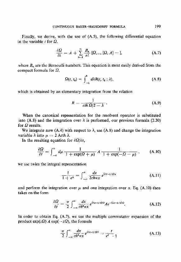
Finally, we derive, with the use of (A,5), the following differential equation in the variable t for Q.

aJ-2 _ = A + -f 1 [Q )..., [fi, A] -*- 1, at n=1 .

(A.71

where B, are the Bernoulli numbers. This equation is most easily derived from the compact formula for L?,

Q(t, to) = j1 dAR(t, t, ; A), 68) -1

which is obtained by an elementary integration from the relation

1 R = cth Ii’/2 - h * (A-9)

When the canonical representation for the resolvent operator is substituted into (A.8) and the integration over h is performed, our previous formula (2.30) for 52 results.

We integrate now (A.4) with respect to X, use (A.8) and change the integration variable X into p = 2 Arth h.

In the resulting equation for X2/i%,

aa s m dP

1 A

1 at= mm 1 + exp(Q + p) 1 + exp(-J2 - CL) ’

(A.10)

we use twice the integral representation

1 mdx -= s

(ix-l/P)Y 1 + eV -,mGe

(A.11)

and perform the integration over ~1 and one integration over x. Eq. (A.10) then takes on the form

aS2 rr m dx -=- 2 -,Ch2?TXe s

(is-1/2)s2

at /&iZ-l/2)" (A.12)

In order to obtain Eq. (A.7), we use the multiple commutator expansion of the product exp(zQ) A exp(-zQ), the formula

rr m s

dx (ix-1iz)t _ t T -,zze

-- et - 1

(A.13)

200 BIALYNICKI-BIRULA, MIELNIK, AND PLEBAhKI

and the definition of the Bernoulli numbers B,, ,

(A. 14)

Differential equation (A.7) has been obtained by Magnus (I) by a completely different method.

REFERENCES

1. W. MAGNUS, Commun. Pure Appl. Math. 7, 649 (1954). 2. W. MAGNUS, A. KARRASS, AND D. SOLITAR, “Combinatorial Group Theory,” Chap. 5.

Interscience, New York, 1966. 3. F. J. DYSON, Phys. Rev. 75, 486 (1949). 4. J. SCHWINGER, Phys. Rev. 74, 1439 (1948). 5. R. M. WILCOX, J. Math. Phys. 8, 962 (1967). 6. G. N. WATSON, “A Treatise on the Theory of Bessel Functions,” Chap. 13. University Press,

Cambridge, 1922. 7. V. DE ALFARO AND T. REGGE, “Potential Scattering,” Chap. 4, North Holland, Amsterdam,

1965.