Embed Size (px)
Citation preview

imagine • explore • learnwww.einsteinworld.com
ALBERT EINSTEIN and EINSTEIN are either trademarks or registered trademarks of The Hebrew University of Jerusalem. Represented exclusively by GreenLight. Official licensed merchandise. Website: einstein.biz © 2014 Fourier Systems Ltd. All rights reserved. Fourier Systems Ltd. logos and all other Fourier product or service names are registered trademarks or trademarks of Fourier Systems. All other registered trademarks or trademarks belong to their respective companies. einstein™World LabMate, einstein™Activity Maker, MultiLab, MiLAB and Terra Nova, are registered trademarks or trademarks of Fourier Systems LTD. First Edition, April 2014.
www.einsteinworld.com
USA8940 W. 192nd St.
Unit IMokenaIL 60448
Tel: (877) 266-4066
www.FourierEdu.com
Israel 16 Hamelacha St.POB 11681Rosh Ha’ayin 48091Tel: +972-3-901-4849 Fax: +972-3-901-4999
Experiments in C
hemistry for M
ultiLab
Experiments in Chemistry for MultiLab™
| 2 |
Table of Contents
Table Of Contents 2
Experiments By Sensors 3
Preface 3
1. Endothermic Reactions: Dissolution Of Ammonium Nitrate In Water 12
2. Endothermic Reactions: Mixing Crystals Of Barium Hydroxide and Ammonium Isothiocyanate 16
3. Endothermic Reactions: Reaction Of Citric Acid Solution With Baking Soda 20
4. Exothermic Reactions: Dissolution Of Naoh In Water 24
5. Acid - Base Titration: Reaction Of NaOH With HCl 28
6. Reduction And Oxidation (Redox) Reactions: Copper Chloride With Aluminum 32
7. Chemical Catalysis: Decomposition Of H2O2 In The Presence Of MnO2 36
8. Hess’s Law: The Conservation Of Energy In Chemistry 40
9. Heat Of Combustion 44
10. Energy Content Of Foods 48
11. Energy Content Of Fuels 52
12. Boyle’s Law 56
13. Effects Of Variations In Air Temperature On Air Pressure: The Combined Gas Law 59
14. Saltwater Conductivity 64
15. The Lambert-Beer Law 67
16. Exploring A Flame 71
17. Freezing And Melting Of Water 74
18. Another Look At Freezing Temperature 77
19. Chemical Equilibrium: Finding A Constant, Kc 80
| 3 |
Experiments by Sensors
Colorimeter
15. The Lambert-Beer Law 67
19. Chemical Equilibrium: Finding a Constant, Kc ERROR! BOOKMARK NOT DEFINED.
Conductivity
14. Saltwater Conductivity 64
pH
5. Acid - Base Titration: Reaction of NaOH with HCl 28
4. Exothermic Reactions: Dissolution of NaOH in Water 24
Pressure (150 –1150 mbar)
7. Chemical Catalysis: Decomposition of H2O2 in the Presence of MnO2Error! Bookmark not defined.
12. Effects of Variations in Air Volume on Air Pressure: Boyle’s Law 56
13. Effects of Variations in Air Temperature on Air Pressure: The Combined Gas LawERROR! BOOKMARK NOT DEFINED.
Temperature (-40 ºC to 140 ºC)
1. Endothermic Reactions: Dissolution Of Ammonium Nitrate In Water 12
2. Endothermic Reactions: Mixing Crystals of Barium Hydroxide and Ammonium Isothiocyanate 16
3. Endothermic Reactions: Reaction of Citric Acid Solution with Baking Soda 20
4. Exothermic Reactions: Dissolution of NaOH in Water 24
5. Acid - Base Titration: Reaction of NaOH with HCl 28
6. Reduction and Oxidation (Redox) Reactions: Copper Chloride with Aluminum 32
8. Hess’s Law: The Conservation of Energy in Chemistry Error! Bookmark not defined.
9. Heat of Combustion 44
10. Energy Content Of Foods 48
11. Energy Content Of Fuels 52

| 4 |
13. Effects of Variations in Air Temperature on Air Pressure: The Combined Gas LawError! Bookmark not defined.
17. Freezing and Melting of Water Error! Bookmark not defined.
10. Another Look at Freezing Temperature Error! Bookmark not defined.
Temperature (0 ºC to 1250 ºC)
16. Exploring a Flame 71

| Preface |
| 5 |
Preface This book contains 20 Chemistry experiments for students designed for use with MultiLab4™, an einstein™ LabMate and einstein™ Sensors. The most recent version of MultiLab4 can be downloaded from the FOURIER Education website. (http://fourieredu.com) For your convenience we have added an index in which the experiments are sorted according to sensor.
einstein™ LabMate The einstein™ LabMate includes the following: 6 built-in sensors:
• Heart Rate • Temperature • Humidity • Pressure • UV • Light + 4 ports for external sensors
External sensors can be connected by inserting the sensor cable into one of the sensor ports.
Connecting the einstein™ LabMate
1. Press the Power button on the top of the device to turn it on
2. When the einstein™ LabMate powers up, it will display either a green, blue or red and green flashing light.
• A blue flashing light indicates that the einstein™ LabMate is on and paired with a computer
• A green flashing light indicates that the einstein™ LabMate is on but not paired with a computer
• A red and green flashing light indicated the einstein™ LabMate is low on battery and should be
plugged into the USB charging cable.
Note: The einstein™ LabMate can also be connected to the computer via a USB cable.
To pair the einstein™LabMate+ with your Windows 7 computer's Bluetooth adaptor 1. First, verify that a Bluetooth adaptor is installed on your computer. If you are not sure how to do this,
please consult the Microsoft Support web pages. Then, pair the einstein™LabMate to your
computer, Here's how:
2. Open Devices and Printers by clicking the Start button ( ), and then, on the Start menu, clicking Devices
and Printers.
3. Click Add a device, and then follow the instructions.

| Preface |
| 6 |
4. Click the einstein™LabMate you want to add to your computer, then click Next. Your einstein™LabMate
should appear in the list of available devices under the name "LabMate" with 3 or four digits directly
after. These digits will match the last 3 or four digits of the serial number of your einstein™LabMate,
located on the back of your device. If you don't see the einstein™LabMate you want to add, make sure the
device is turned on. If you just turned on the device, it may take Windows several seconds to detect it.
Note: If you are using a Windows version other than Windows 7, please consult the Microsoft Support pages on how to pair a Bluetooth device to your computer.
Pairing einstein™LabMate with your Mac via bluetooth 1. Make sure that your computer has Bluetooth
Make sure that your computer has Bluetooth built-in or that a compatible Bluetooth adapter is connected.
Open System Preferences (from the Apple menu, choose System Preferences), then choose Bluetooth from
the View menu.
2. Turn on Bluetooth
In Bluetooth preferences, select the "On" checkbox (for earlier Mac OS X versions, click the Settings tab,
then click Bluetooth Power: On). Make sure to also turn on your einstein™LabMate
3. Set up a new device
Click “Set Up New Device” (in earlier Mac OS X versions, click the Devices tab in Bluetooth, then click "Set
Up New Device"). Your einstein™LabMate should appear in the list of available devices under the name
"LabMate" with 3 or four digits directly after. These digits will match the last 3 or four digits of the serial
number of your einstein™LabMate, located on the back of your device. If you don't see the
einstein™LabMate you want to add, make sure the device is turned on. Follow the onscreen instructions to
finish setting up your einstein™LabMate.
MultiLab4 setup
When using the einstein™ Labmate, select the MultiLab4 icon ( ) on the application desktop.
If you are in a room where others are using einstein™ LabMates, make sure you are paired with your einstein™ LabMate. The serial number appearing in the lower right of the MultiLab4™ screen should match that on the underside of your einstein™ LabMate device.

| Preface |
| 7 |
Working with Graphs in MultiLab4 The experiments in this book require the use of the MultiLab4 program to analyze the results.
Understanding Graphs
In general, graphs in MultiLab4 represent the data from one or more sensors along the y (horizontal) axis vs. time along the x (vertical) axis. It is also possible to display data from one sensor along the x axis. To change what is displayed along the x axis, click on the arrow key ( ) below the x axis. Choose any data set from the drop down menu. By default, graphs in MultiLab4 auto scale, which means you can see the entire graph displayed. Graph Toolbar:
To zoom in on one part of the graph, use the Zoom tool ( ) from the graph toolbar at the bottom of the graph window. Drag the cursor over the region of the graph you want to expand. Click the Zoom tool again to disable the zoom feature. Click on the Autoscale tool ( ) to return to the original auto scale graph. You can also move the graph using the Pan tool ( ).
Analyzing a Graph
Analyzing the information contained in a graph is one of MultiLab4’s most important and powerful functions. To analyze a graph: • Run an Experiment.
• In order to use most of MultiLab4’s analysis functions, you must select at least one point on the graph – this
is known as a cursor. Many functions require two cursors. Use the cursor tools to display first one and
then two cursors.
Note: If you are using more than one sensor, both points will appear on the same plot line.
Working with Cursors
You can display up to two cursors on the graph simultaneously. Use one cursor to display individual data recording values or to select a curve. Use two cursors to analyze the data in the graph. 1. To display the first cursor:
In the graph window, click on any point on a plot line. MultiLab4 will now display the coordinate values.
| Preface |
| 8 |
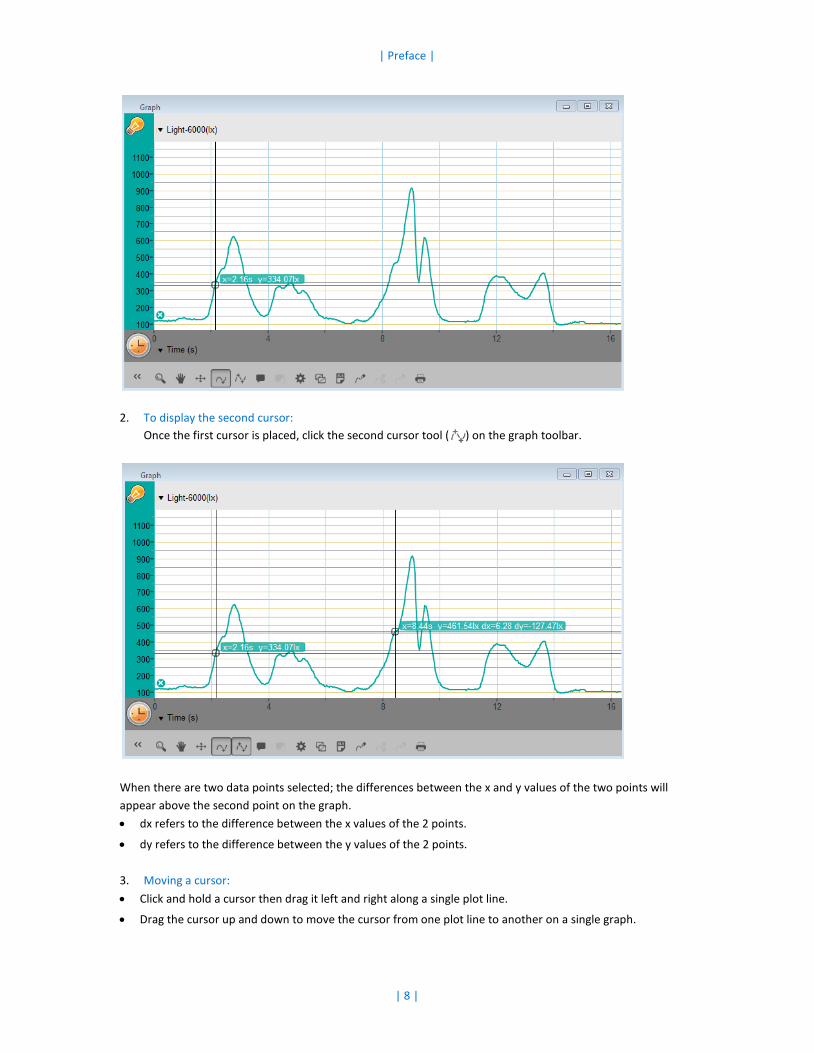
2. To display the second cursor: Once the first cursor is placed, click the second cursor tool ( ) on the graph toolbar.
When there are two data points selected; the differences between the x and y values of the two points will appear above the second point on the graph. • dx refers to the difference between the x values of the 2 points.
• dy refers to the difference between the y values of the 2 points.
3. Moving a cursor: • Click and hold a cursor then drag it left and right along a single plot line.
• Drag the cursor up and down to move the cursor from one plot line to another on a single graph.

| Preface |
| 9 |
4. To remove a cursor: • Click on the second and then the first cursor tool on the graph toolbar.
The cursors will disappear from the plot line
Working with Functions
Once you have selected a cursor, many powerful analysis tools are available. Select the Analysis toolbar to access the list of tools available to you.
Select one of the analysis tools to apply it to your data. Some of the analysis tools will draw a new plot line on the graph, displaying the results. The Math Functions tool ( ) will allow you to perform mathematical operations on your data.
Select this tool to open the Math Function window and choose the mathematical operation from the dropdown Function menu. You can choose your data set from the dropdown menu G1. An equation representing the mathematical operation will appear in bold in the Math Function window.
Some functions, such as Subtract, require you to compare 2 plot lines. To compare two plot lines: • Use the G1 and G2 dropdown menus to select the plot lines you would like to compare.
• Select Ok.
• A new plot line will appear on the graph, displaying the results.
Experimental Layout Each experiment includes the following parts: • Introduction: A brief description of the concept and theory
| Preface |
| 10 |
• Equipment: The equipment needed for the experiment
• Equipment Setup: Illustrated guide to assembling the experiment
• Current Setup Summary: Recommended setup
• Procedure: Step-by-step guide to executing the experiment
• Data Analysis
• Questions
• Further Suggestions
Sealing Many of the experiments in this book, especially those involving pressure measurements, are dependent on the flasks or test tubes being tightly sealed. Following is a guide to ensure that these experiments run smoothly. Note: To ensure a tight seal you may need to use a material such as modeling clay to seal any openings. Note: You may want to consider purchasing the einstein™ Pressure Kit which is specifically designed for these types of experiments. Once you have sealed the flask or test tube, you can test the seal.
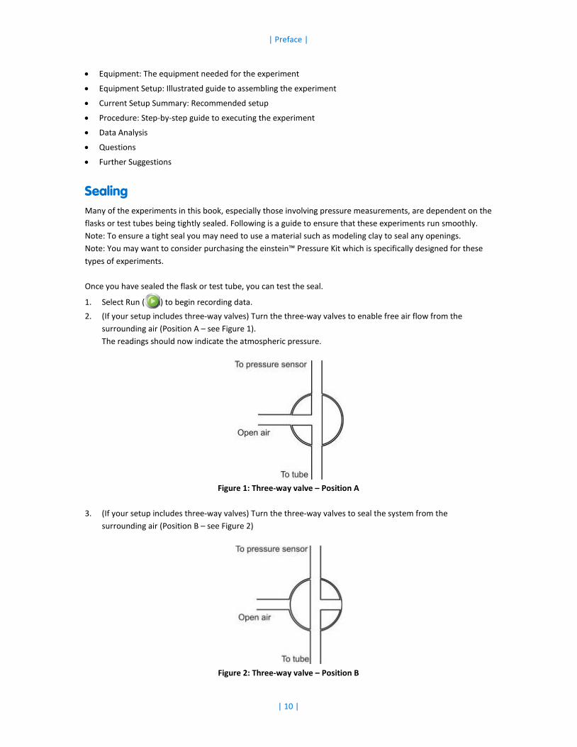
1. Select Run ( ) to begin recording data. 2. (If your setup includes three-way valves) Turn the three-way valves to enable free air flow from the
surrounding air (Position A – see Figure 1). The readings should now indicate the atmospheric pressure.
Figure 1: Three-way valve – Position A
3. (If your setup includes three-way valves) Turn the three-way valves to seal the system from the
surrounding air (Position B – see Figure 2)
Figure 2: Three-way valve – Position B

| Preface |
| 11 |
4. Press the stoppers. The pressure should rise a little and then remain constant (see Figure 3).
Figure 3
5. If the pressure drops (see Figure 4), there is a leak. Check your seals carefully and use a material such as
modeling clay to seal off any possible openings. Repeat step 4. If that doesn’t help, replace the stopper.
Figure 4
6. After you are satisfied that the containers are sealed, select Stop ( ).
Safety Precautions • Follow standard safety procedures for laboratory activities in a science classroom.
• Proper safety precautions must be taken to protect teachers and students during the experiments
described in this book.
• It is not possible to include every safety precaution or warning!
• Fourier assumes no responsibility or liability for use of the equipment, materials,
or descriptions in this book.
Pres
sure
(mba
r)
Pr
essu
re (m
bar)

| Endothermic Reactions: Dissolution of Ammonium Nitrate in Water |
| 12 |
Chapter 1
Endothermic Reactions: Dissolution of Ammonium Nitrate in Water
Figure 1
Introduction
An endothermic process is a chemical reaction in which heat is absorbed. When we perform an endothermic reaction in a flask, it initially cools. Later, heat from the surroundings flows to the flask until a temperature balance is established. In this experiment we follow temperature changes occurring during the dissolution of crystalline ammonium nitrate in water.The heat of the reaction can be calculated using the following equation:
𝑄 = 𝑚𝐶∆𝑇 (1)
Where: Q = The quantity of heat released or absorbed. m = The mass of the substance. C = The heat capacity of the substance. ∆T =The change in temperature.
| Endothermic Reactions: Dissolution of Ammonium Nitrate in Water |
| 13 |
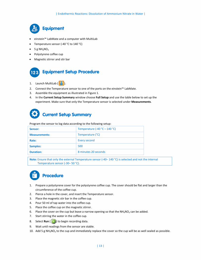
Equipment
• einstein™ LabMate and a computer with MultiLab
• Temperature sensor (-40 °C to 140 °C)
• 5 g NH4NO3
• Polystyrene coffee cup
• Magnetic stirrer and stir bar
Equipment Setup Procedure
1. Launch MultiLab ( ).
2. Connect the Temperature sensor to one of the ports on the einstein™ LabMate. 3. Assemble the equipment as illustrated in Figure 1. 4. In the Current Setup Summary window choose Full Setup and use the table below to set up the
experiment. Make sure that only the Temperature sensor is selected under Measurements.
Current Setup Summary
Program the sensor to log data according to the following setup:
Sensor: Temperature (-40 °C – 140 °C)
Measurements: Temperature (°C)
Rate: Every second
Samples: 500
Duration: 8 minutes 20 seconds
Note: Ensure that only the external Temperature sensor (-40– 140 °C) is selected and not the internal Temperature sensor (-30– 50 °C).
Procedure
1. Prepare a polystyrene cover for the polystyrene coffee cup. The cover should be flat and larger than the circumference of the coffee cup.
2. Pierce a hole in the cover, and insert the Temperature sensor. 3. Place the magnetic stir bar in the coffee cup. 4. Pour 50 ml of tap water into the coffee cup. 5. Place the coffee cup on the magnetic stirrer. 6. Place the cover on the cup but leave a narrow opening so that the NH4NO3 can be added. 7. Start stirring the water in the coffee cup.
8. Select Run ( ) to begin recording data.
9. Wait until readings from the sensor are stable. 10. Add 5 g NH4NO3 to the cup and immediately replace the cover so the cup will be as well sealed as possible.

| Endothermic Reactions: Dissolution of Ammonium Nitrate in Water |
| 14 |
11. Follow the changes in temperature in the Graph window of MultiLab until no further changes in temperature are observed.
12. Select Stop ( ) to stop collecting data.
13. Save your data by selecting Save ( ) from the Basic Tools window on the upper menu bar.
Data Analysis
For more information on working with graphs see: Working with Graphs in MultiLab. 1. On the graph, use the cursors to select the starting temperature and the the final temperature. 2. How did the temperature change during the dissolution of crystalline ammonium nitrate in water? 3. What is the difference between the two values? 4. How long did it take for the reaction to reach the final temperature? 5. Calculate the heat of the reaction using equation 1.
Note: The specific heat capacity of water at 25 °C is 4.18 J/g °C.
An example of the graph of Temperature vs. Time obtained in this experiment is shown below:
Figure 2
Tem
pera
ture
(0 C)

| Endothermic Reactions: Dissolution of Ammonium Nitrate in Water |
| 15 |
Questions
1. What kind of chemical reaction is the dissolution of ammonium nitrate in water? Base your conclusions on your observations made during the experiment you performed.
2. Try to predict the results of the dissolution of different amounts of NH4NO3 in water. How would the temperature change be effected?
3. What would be the effect of warming the water prior to the dissolution of NH4NO3? What would be the effect of cooling the water?
Further Suggestions
1. Dissolve different amounts of NH4NO3 in water. Follow changes in temperature in each case. Calculate the heat of the reaction in each case.
2. Examine the effect of increasing and decreasing the initial temperature of the water on the dissolution of NH4NO3.

| 16 |
Chapter 2
Endothermic Reactions: Mixing Crystals of Barium Hydroxide
and Ammonium Isothiocyanate
Figure 1
Introduction
When the two crystalline substances Ba(OH)2·8H2O and NH4SCN are thoroughly mixed in a flask, a heat absorbing or endothermic reaction occurs:
Ba(OH)2 ∙ 8H2O + 2NH4SCN ⟶ Ba(SCN)2 + 2NH3 + 10H2O (1)
The gaseous substance ammonia (NH3), formed in this reaction, can easily be detected due to its pungent smell. If the flask, which feels very cold to the touch, is set on a board covered with a thin layer of water, the flask and board freeze together. In this experiment we follow temperature changes that occur upon mixing crystalline barium hydroxide octahydrate with ammonium isothiocyanate. We also observe the reaction flask and the board freezing together as a result of the cooling which occurs during an endothermic reaction. The heat of the reaction can be calculated using the following equation:

| Endothermic Reactions: Mixing Crystals of Barium Hydroxide and Ammonium Isothiocyanate |
| 17 |
𝑄 = 𝑚𝐶∆𝑇 (2)
Where: Q = The quantity of heat released or absorbed. m = The mass of the substance. C = The heat capacity of the substance. ∆T =The change in temperature.
Equipment
• einstein™ LabMate and a computer with MultiLab • Temperature sensor (-40 °C to 140 °C) • 2 g of Ba(OH)2 ·8H2O • 4 g of NH4SCN • Wooden or a plastic board, approximately 5 cm x 5 cm • 10 ml glass flask • 10 cm glass rod
Equipment Setup Procedure
1. Launch MultiLab ( ).
2. Connect the Temperature sensor to one of the ports on the einstein™ LabMate. 3. Assemble the equipment as illustrated in Figure 1. 4. In the Current Setup Summary window choose Full Setup and use the table below to set up the
experiment. Make sure that only the Temperature sensor is selected under Measurements.
Current Setup Summary
Program the sensor to log data according to the following setup:
Sensor: Temperature (-40 °C – 140 °C)
Measurements: Temperature (°C)
Rate: Every second
Samples: 200
Duration: 3 minutes 20 seconds
Note: Ensure that only the external Temperature sensor (-40– 140 °C) is selected and not the internal Temperature sensor (-30– 50 °C).

| Endothermic Reactions: Mixing Crystals of Barium Hydroxide and Ammonium Isothiocyanate |
| 18 |
Procedure
1. Pour water on the board until it is covered with a thin layer of water(see Figure 1). 2. Weigh 2 g of Ba(OH)2·8H2O into the 10 ml glass flask. 3. Weigh 4 g of ammonium isothiocyanate and set it aside. 4. Insert the Temperature sensor into the barium hydroxide crystals in the flask.
5. Select Run ( ) to begin recording data.
6. Wait until readings from the Temperature sensor are stable. 7. Add the weighed NH4SCN to the flask containing the Ba(OH)2·8H2O. 8. Place the flask on the water covered board as shown in Figure 1B.
Figure 1a
9. Thoroughly mix the substances in the flask using the glass rod. 10. Follow the changes in temperature in the flask in the Graph window of MultiLab until no further changes in
temperature are observed.
11. When the temperature stabilizes, select Stop ( ) to stop collecting data.
12. Save your data by selecting Save ( ) from the Basic Tools window on the upper menu bar.
13. Try to remove the flask from the board.
Data Analysis
For more information on working with graphs see: Working with Graphs in MultiLab 1. On the graph, use the cursors to select the initial temperature and the final temperature. How did the
temperature change during this chemical reaction? What is the difference between the two values?

| Endothermic Reactions: Mixing Crystals of Barium Hydroxide and Ammonium Isothiocyanate |
| 19 |
2. How long did it take for the reaction to reach the final temperature? Calculate the heat of reaction using equation 2.
Note: The specific heat capacity of water at 25 °C is 4.18 J/g °C.
3. Describe what happened when you tried to pick up the flask. An example of the Temperature vs. Time graph obtained in this experiment is shown in the graph below.
Figure 2
Questions
1. What changes in the temperature of the flask did you observe? Explain your results. 2. What kind of chemical reaction occurred in the flask? 3. Explain what happened when you tried to lift up the flask.
Further Suggestions
1. Change the relative amounts of Ba(OH)2·8H2O and NH4SCN and follow the temperature change in each case.
2. Perform an additional endothermic reaction: Dissolution of KNO3 in water (25 g in 50 ml water). 3. Follow the rate of ammonium release in the reaction, using a Pressure sensor. In this way the reaction rate
can be measured.
Tem
pera
ture
(0 C)

| 20 |
Chapter 3
Endothermic Reactions: Reaction of Citric Acid Solution with Baking Soda
Figure 1
Introduction
An endothermic process is a chemical reaction in which heat is absorbed. When we perform an endothermic reaction in a flask, it initially cools. Later, heat from the surroundings flows to the flask until temperature balance is established. In this experiment we follow temperature changes occurring during the reaction between a citric acid solution and baking soda.
H3C6H5O7 (aq) + 3NaHCO3 (s) ⟶ 3CO2 (g) + 3H2O + Na3C6H5O7 (aq) (1)
The heat of the reaction can be calculated using the following equation:
𝑄 = 𝑚𝐶∆𝑇 (2)
Where: Q = The quantity of heat released or absorbed. m = The mass of the substance. C = The heat capacity of the substance. ∆T =The change in temperature.

| Endothermic Reactions: Reaction of Citric Acid Solution with Baking Soda |
| 21 |
Equipment
• einstein™ LabMate and a computer with MultiLab • Temperature sensor (-40 °C to 140 °C) • 25 ml citric acid (H3C6H5O7) solution • 15 g baking soda (NaHCO3) • Polystyrene coffee cup • Magnetic stirrer and stir bar • Safety goggles
Equipment Setup Procedure
1. Launch MultiLab ( ).
2. Connect the Temperature sensor to one of the ports on the einstein™ LabMate. 3. Assemble the equipment as illustrated in Figure 1. 4. In the Current Setup Summary window choose Full Setup and use the table below to set up the
experiment. Make sure that only the Temperature sensor is selected under Measurements.
Current Setup Summary
Program the sensor to log data according to the following setup:
Sensor: Temperature (-40 °C – 140 °C)
Measurements: Temperature (°C)
Rate: Every second
Samples: 500
Duration: 8 minutes 20 seconds
Note: Ensure that only the external Temperature sensor (-40– 140 °C) is selected and not the internal Temperature sensor (-30– 50 °C).

| Endothermic Reactions: Reaction of Citric Acid Solution with Baking Soda |
| 22 |
Procedure
Always wear safety goggles. 1. Prepare a polystyrene cover for the polystyrene coffee cup. The cover should be flat and larger than the
circumference of the coffee cup. 2. Pierce a hole in the cover, and insert the Temperature sensor. 3. Place the magnetic stir bar in the coffee cup. 4. Pour 25 ml of citric acid into the coffee cup. 5. Place the coffee cup on the magnetic stirrer. 6. Place the cover on the cup, but leave a narrow opening so that the baking soda (NaHCO3) can be added. 7. Start stirring the water in the coffee cup.
8. Select Run ( ) to begin recording data. Wait until readings from the sensor are stable.
9. After 20 seconds add the baking soda (NaHCO3) to the cup and immediately replace the cover to ensure that the cup is sealed.
10. Follow the changes in temperature in the Graph window of MultiLab until no further changes in temperature are observed.
11. Select Stop ( ) to stop collecting data.
12. Save your data by selecting Save ( ) from the Basic Tools window on the upper menu bar.
Data Analysis
For more information on working with graphs see: Working with Graphs in MultiLab 1. On the graph, use the cursors to select the initial temperature and the final temperature. How did the
temperature change during this chemical reaction? What is the difference between the two values? 2. How long did it take for the reaction to reach the final temperature?
Calculate the heat of the reaction using equation 2.

| Endothermic Reactions: Reaction of Citric Acid Solution with Baking Soda |
| 23 |
An example of the Temperature vs. Time graph obtained in this experiment is shown below:
Figure 2
Questions
1. What kind of chemical reaction takes place when mixing citric acid solution and baking soda? Base your conclusions on your observations from the experiment you performed.
2. Try to predict the results of mixing different amounts of baking soda in a citric acid solution. What will be the extent of the temperature change?
Further Suggestions
1. Change the relative amounts of citric acid and baking soda. Follow changes in temperature in each case. Calculate the heat of reaction in each case.
2. Follow the rate of CO2 release in the reaction using the CO2 sensor.
Tem
pera
ture
(0 C)

| 24 |
Chapter 4
Exothermic Reactions: Dissolution of NaOH in Water
Figure 1
Introduction
Nearly all chemical reactions involve either the release or absorption of heat. These reactions are classified as either exothermic or endothermic. An exothermic process is a chemical reaction in which heat is generated. When we perform an exothermic reaction in a flask, it initially warms. Later, heat from the flask flows to the surrounding air until a temperature balance is established. A calorimeter is the device used to measure the heat absorbed or generated during a chemical reaction. The heat of reaction can be calculated using the following equation:
𝑄 = 𝑚𝐶∆𝑇 (1)
Where: Q = The quantity of heat released or absorbed. m = The mass of the substance. C = The heat capacity of the substance. ∆T =The change in temperature. In this experiment we follow the temperature changes that occur during the dissolution of sodium hydroxide in water. A polystyrene coffee cup will serve as a calorimeter.

| Exothermic Reactions: Dissolution of NaOH in Water|
| 25 |
Equipment
• einstein™ LabMate and a computer with MultiLab
• pH sensor
• Temperature sensor (-40 °C to 140 °C)
• Polystyrene coffee cup
• 10 g NaOH
• Magnetic stirrer and stir bar
Equipment Setup Procedure
1. Launch MultiLab ( ).
2. Connect the pH sensor to one of the ports on the einstein™ LabMate. 3. Connect the Temperature sensor to one of the ports on the einstein™ LabMate. 4. In the Current Setup Summary window choose Full Setup and use the table below to set up the
experiment. Make sure that only the pH and Temperature sensors are selected under Measurements.
Current Setup Summary
Program the sensors to log data according to the following setup:
Sensor: pH 0-14
Measurements: pH
Sensor: Temperature (-40 °C – 140 °C)
Measurements: Temperature (°C)
Rate: Every second
Samples: 5000
Duration: 1 hour 23 minutes 20 seconds
Note: Ensure that only the external Temperature sensor (-40– 140 °C) is selected and not the internal Temperature sensor (-30– 50 °C).
Procedure
1. Prepare a polystyrene cover for the polystyrene coffee cup. The cover should be flat and larger than the circumference of the coffee cup (see Figure 1).
2. Pierce two holes in the cover: one for the pH electrode, one for the Temperature sensor. 3. Place the magnetic stir bar in the coffee cup. 4. Pour 100 ml of tap water into the coffee cup. 5. Place the coffee cup on the magnetic stirrer. 6. Place the cover on the cup, but leave a narrow opening so that NaOH can be added. 7. Start stirring the water in the coffee cup.

| Exothermic Reactions: Dissolution of NaOH in Water|
| 26 |
8. Select Run ( ) to begin recording data.
9. Start stirring the water in the coffee cup. 10. Wait until readings from the sensors are stable. 11. Add 2 g crystalline NaOH to the cup and immediately adjust the cover so that the cup is sealed as well as
possible. 12. Follow changes in pH and temperature in the Graph window of MultiLab until the readings stabilize.
13. Select Stop ( ) to stop collecting data.
14. Save your data by selecting Save ( ) from the Basic Tools window on the upper menu bar.
Data Analysis
For more information on working with graphs see: Working with Graphs in MultiLab 1. How did the pH change during the dissolution process?
On the graph, use the cursors to select the initial pH value and then the final pH value. a. Note the difference between the two values. b. Note how much time it took to reach the final pH value. c. Note the difference between the two pH values.
2. On the graph, use the cursors to determine the temperature change during the process. 3. Calculate the heat of the reaction using the temperature change you determine (∆T) and equation 1.
Note: The specific heat capacity of water at 25 °C is 4.18 J/g °C.
An example of the graph obtained in this experiment is shown below:
Figure 2
pH
Temp
Tem
pera
ture
(0 C)
pH
14
13
12
11
10
9
8
7
6
| Exothermic Reactions: Dissolution of NaOH in Water|
| 27 |
Questions
1. Was the pH change fast? Compare the time span of the pH changes with that of the temperature changes. 2. Explain the difference in the time span needed for the pH changes and the temperature changes. 3. Is the dissolution of NaOH an exothermic or endothermic reaction? Is it a vigorous reaction? Base your
conclusions on your observations of the experiment you performed. 4. Try to guess what the results of the dissolution would be if you added different amounts of NaOH to the
water. What would the pH change be in each case? What would be the extent of change in the temperature?
Further Suggestions
1. Dissolve different amounts of NaOH in water. Follow changes in pH and temperature in each case. Calculate the heat of the reaction in each case.
2. Examine the effect of the pH of the water on the dissolution of NaOH. Follow the heat of the reaction in a buffer solution. Alternatively, dissolve KOH or NH4OH in the water before dissolving the NaOH.
3. Perform an additional exothermic reaction. Dissolve anhydrous CuSO4 (white crystals) in water. Dissolution of Copper Sulfate in water forms a blue hydrated copper ion.

| 28 |
Chapter 5
Acid - Base Titration: Reaction of NaOH with HCl
Figure 1
Introduction
In aqueous solutions, adding bases to water leads to an increase in the pH of the solution, while the addition of acids leads to a decrease in the pH. The changes in the pH can be followed using either specific dyes, called indicators, or a pH electrode. Acids and bases neutralize, or reverse, the action of one another. By adding a known amount of acid to a basic solution whose concentration is not known, until it completely neutralizes it, the amount of the base can be determined. This procedure is called: Acid - Base Titration. During neutralization, acids and bases react with each other to produce ionic substances, called salts. In this experiment, changes in pH and temperature, occurring while an acid (hydrochloric acid, (Hcl)) is added to a base (sodium hydroxide (NaOH)) solution, are followed using a pH electrode and a Temperature sensor.

| Acid - Base Titration: Reaction of NaOH with HCl |
| 29 |
Equipment
• einstein™ LabMate and a computer with MultiLab
• pH sensor
• Temperature sensor (-40 °C to 140 °C)
• Polystyrene coffee cup
• 50 ml burette
• Glass funnel
• 50 ml of 0.5N NaOH (approximately)
• 100 ml of 1N HCl solution
• Safety goggles and gloves
• Magnetic stirrer and stir bar
Equipment Setup Procedure
1. Launch MultiLab ( ).
2. Connect the pH sensor to one of the ports on the einstein™ LabMate. 3. Connect the Temperature sensor to one of the ports on the einstein™ LabMate. 4. Assemble the equipment as illustrated in Figure 1. 5. In the Current Setup Summary window choose Full Setup and use the table below to set up the
experiment. Make sure that only the pH and Temperature sensors are selected under Measurements.
Current Setup Summary
Program the sensors to log data according to the following setup:
Sensor: pH 0-14
Measurements: pH
Sensor: Temperature (-40 °C – 140 °C)
Measurements: Temperature (°C)
Rate: Every second
Samples: 2000
Duration: 33 minutes 20 seconds
Note: Ensure that only the external Temperature sensor (-40– 140 °C) is selected and not the internal Temperature sensor (-30– 50 °C).

| Acid - Base Titration: Reaction of NaOH with HCl |
| 30 |
Procedure
1. Prepare a polystyrene cover for the polystyrene coffee cup. The cover should be flat and larger than the circumference of the coffee cup (see Figure 1).
2. Pierce three holes in the cover: one for the pH electrode, one for the Temperature sensor and one for the glass funnel.
3. Place the magnetic stir bar in the coffee cup. 4. Add 50 ml of the 0.5 N NaOH solution to the coffee cup. 5. Place the coffee cup on the magnetic stirrer. 6. Place the cover on the cup. 7. Start stirring the NaOH solution in the coffee cup.
8. Select Run ( ) to begin recording data. 9. Wait until readings from the sensors are stable. 10. Add, drop-by-drop, 1 N HCl solution from the burette to the cup, through the glass funnel . 11. Follow changes in pH and temperature in the Graph window of MultiLab. 12. As the pH just starts to change, stop the drip of HCl and note the volume of HCl added until that point. 13. Renew the drop-by-drop addition of HCl, following pH changes very carefully. 14. Stop the flow of HCl as soon as the pH level stabilizes.
15. Save your data by selecting Save ( ) from the Basic Tools window on the upper menu bar.
Data Analysis
For more information on working with graphs see: Working with Graphs in MultiLab 1. On the graph, use the cursors to measure the initial pH value of the solution and the final pH value. 2. How did the pH change during the neutralization process? What was the volume of HCl added when the pH
started to change? Compare it to the volume of HCl added when the NaOH was completely neutralized. 3. On the graph, select the time when the pH began to change and then select the point of neutralization.
How much time did it take? 4. On the graph, select the initial temperature and the final temperature. How did the temperature change? 5. Calculate the heat of reaction Q,
𝑄 = 𝑚𝐶𝑝∆𝑇 (1)
Where:
m = The mass of the water Cp = The heat capacity of water at constant pressure ΔT = The change in temperature
Note: The specific heat capacity of water at 25 °C is 4.18 J/g °C.

| Acid - Base Titration: Reaction of NaOH with HCl |
| 31 |
An example of the graph obtained in this experiment is shown below:
Figure 2
Questions
1. Did you observe a fast pH change? Explain the difference in the short time interval needed for the completion of the drastic changes of pH and that of the whole neutralization process.
2. Is the neutralization reaction an exothermic or endothermic reaction? Base your conclusions on the experiment you performed.
3. Try to predict what would happen if you did the acid - base titration with different concentrations of NaOH in the coffee cup. What would be the pH change in each case? What would be the extent of change in the temperature?
4. What will be the effect of reacting other acids (such as, for example, acetic acid) with NaOH?
Further Suggestions
1. Use different concentrations of NaOH with a constant concentration of HCl. 2. Calculate unknown concentrations of the titrated NaOH (or HCl). This can be done by setting the flow of
acid (or base) from the burette pipette at a constant rate. Use this flow rate together with the time data from your graph to calculate the amount of titrant added to the solution.
3. Perform acid-base titrations with different types of acids and/or bases: A weak acid with a strong base and vice versa.
pH
Temp pH
30
28
26
24
22
20
18
16
14

| 32 |
Chapter 6
Reduction and Oxidation (Redox) Reactions: Copper Chloride
with Aluminum
Figure 1
Introduction
Redox reactions involve the transfer of electrons between two chemicals. The compound that loses an electron is said to be oxidized, the one that gains an electron is said to be reduced. A compound that is oxidized is referred to as a reducing agent while a compound that is reduced is referred to as an oxidizing agent. In this experiment we will be following the temperature changes that occur during redox reaction:
2Al(s)0 + 3Cu(aq)
2+ + 6Cl(aq)− ⟶ 2Al(aq)
3+ + 3Cu(s)0 + 6Cl(aq)
− (1)
Aluminum, Al, is oxidized from Al0 to Al3+ and copper,Cu, is reduced from Cu2+to Cu0. The heat of the reaction can be calculated using the following equation:
𝑄 = 𝑚𝐶∆𝑇 (2)

| Reduction and Oxidation (Redox) Reactions: Copper Chloride with Aluminum |
| 33 |
Where: Q = The quantity of heat released or absorbed. m = The mass of the substance. C = The heat capacity of the substance. ∆T =The change in temperature.
Equipment
1. einstein™ LabMate and a computer with MultiLab 2. Temperature sensor (-40 °C to 140 °C) 3. Polystyrene coffee cup 4. 5 g CuCl2 5. Magnetic stirrer and stir bar 6. Aluminum foil 7. Safety goggles
Equipment Setup Procedure
1. Launch MultiLab ( ).
2. Connect the Temperature sensor to one of the ports on the einstein™ LabMate. 3. Assemble the equipment as illustrated in Figure 1. 4. In the Current Setup Summary window choose Full Setup and use the table below to set up the
experiment. Make sure that only the Temperature sensor is selected under Measurements.
Current Setup Summary
Program the sensor to log data according to the following setup:
Sensor: Temperature (-40 °C – 140 °C)
Measurements: Temperature (°C)
Rate: Every second
Samples: 200
Duration: 3 minutes 20 seconds
Note: Ensure that only the external Temperature sensor (-40– 140 °C) is selected and not the internal Temperature sensor (-30– 50 °C).

| Reduction and Oxidation (Redox) Reactions: Copper Chloride with Aluminum |
| 34 |
Procedure
Always wear safety goggles. 1. Prepare a polystyrene cover for the polystyrene coffee cup. The cover should be flat and larger than the
circumference of the coffee cup (see Figure 1). 2. Place the magnetic stir bar in the coffee cup. 3. Pour 50 ml of tap water into the coffee cup. 4. Place the coffee cup on the magnetic stirrer. 5. Place the cover on the cup but leave a narrow opening so that CuCl2 can be added. 6. Start stirring the water in the coffee cup.
7. Select Run ( ) to begin recording data. Wait until readings from the sensor are stable.
8. Add 5 g CuCl2 to the cup and immediately replace the cover so the cup will be as well sealed as possible. 9. Add the aluminum foil to the cup and immediately replace the cover so the cup will be as well sealed as
possible. 10. Follow the changes in temperature in the Graph window of MultiLab until no further changes in
temperature are observed.
11. Select Stop ( ) to stop collecting data.
12. Save your data by selecting Save ( ) from the Basic Tools window on the upper menu bar.
Data Analysis
For more information on working with graphs see: Working with Graphs in MultiLab 1. On the graph, use the cursors to select the initial and final temperatures. What is the difference between
them? How did the temperature change during the redox reaction? How long did it take for the reaction to reach the final temperature?
2. Calculate the heat of reaction using equation 2.
Note: The specific heat capacity of water at 25 °C is 4.18 J/g °C.

| Reduction and Oxidation (Redox) Reactions: Copper Chloride with Aluminum |
| 35 |
An example of the graph of Temperature vs. Time obtained in this experiment is shown below:
Figure 2
Questions
1. What changes occurred in the color of the aluminum foil? 2. Write the reaction that took place and write the individual redox reaction equations for copper and
aluminum. 3. Which species was reduced and which was oxidized?
Further Suggestions
1. Drop a piece of iron into a solution of copper chloride. Write the reaction that occurs, and the individual redox equations.
2. Drop a piece of zinc metal into dilute hydrochloric acid. Hydrogen (H2) is given off. Write the general reaction equation and the individual redox equations for this reaction. Which species is reduced? Which species is oxidized?
Tem
pera
ture
(0 C)

| 36 |
Chapter 7
Chemical Catalysis: Decomposition of H2O2 in the Presence of MnO2
Figure 1
Introduction
A catalyst is a chemical that increases the rate of a reaction but is not consumed by the reaction. This process is called catalysis. The catalyst enters the reaction in one step and is regenerated in another step. A pure solution of H2O2 is stable. But when a catalyst, such as MnO2, platinum metal or Fe+2 ions are added, H2O2 rapidly disproportionate to form water and molecular oxygen.
2H2O2 MnO2�⎯⎯� H2O + O2 (1)
In this experiment we use a Pressure sensor to follow the release of molecular oxygen resulting from the disproportionation of H2O2 in the presence of MnO2.

| Chemical Catalysis: Decomposition of H2O2 in the Presence of MnO2 |
| 37 |
Equipment • einstein™ LabMate and a computer with MultiLab • Two Pressure sensors (150 – 1150 mbar) • Two three-way valves • Two 10 ml glass bottles • Two rubber corks, one for each of the bottles • One 2 ml plastic syringe • Three 20-gauge syringe needles • Three short latex tubes • 3% H2O2 solution • A few crystals of MnO2
Equipment Setup Procedure
1. Launch MultiLab ( ).
2. Connect the Pressure sensors to ports on the einstein™ LabMate. 3. Assemble the equipment as illustrated in Figure 1. 4. A syringe needle (20-gauge) is inserted through the cork, until its tip projects out slightly . 5. At the other end of the syringe needle, projecting out of the upper side of the cork, attach a three-way
valve to the pressure sensor. 6. Turn the valve until its opening is directed vertically. In this position, air can flow through the valve.. 7. Insert an additional needle into one of the corks. A syringe filled with 3% H2O2 solution will be attached to
this needle later. 8. In the Current Setup Summary window choose Full Setup and use the table below to set up the
experiment. Make sure that only the Pressure sensors are selected under Measurements.
Current Setup Summary
Program the sensors to log data according to the following setup:
Sensor: Pressure 150 - 1150 mbar
Measurements: Pressure (mbar)
Sensor: Pressure 150 - 1150 mbar
Measurements: Pressure (mbar)
Rate: Every second
Samples: 500
Duration: 8 minutes 20 seconds
Note: Ensure that only the external Pressure sensors (150– 1150 mbar) are selected and not the internal Pressure sensor (0– 400 kPa).

| Chemical Catalysis: Decomposition of H2O2 in the Presence of MnO2 |
| 38 |
Procedure
1. Mark the bottles with labels 1 and 2. 2. Fill the plastic syringe with 2 ml of 3% H2O2 solution. 3. Add 8 ml water and 2 ml 3% H2O2 solution to bottle 1. 4. Add 8 ml water and a few crystals of MnO2 to bottle 2. Gently mix the solution. 5. Close the bottles tightly with the rubber corks. 6. Attach the syringe filled with H2O2 solution to bottle 2 through the additional needle inserted through
the cork.
7. Select Run ( ) to begin recording data.
8. Follow the pressure level in the Graph window of MultiLab. 9. Check that the air in the flasks is at atmospheric pressure (about 1000 mbar). 10. Inject the H2O2 solution into bottle 2 and immediately turn the valves of the two bottles to stop air flow
through them. 11. Follow changes in the pressure levels in the Graph window of MultiLab during the experiment until no
further changes in pressure are observed.
12. Select Stop ( ) to stop collecting data.
13. Save your data by selecting Save ( ) from the Basic Tools window on the upper menu bar.
Data Analysis
For more information on working with graphs see: Working with Graphs in MultiLab 1. On the graph, use the cursors to select the initial pressure and the final pressure from bottle 1. Do the
same for the second bottle. 2. How did the pressure change in each of the bottles? 3. Find the difference between the two sets of values. 4. Calculate the reaction rate of H2O2 disproportionation. Subtract the Pressure graph of the control flask
from that of the experimental flask: a. Use the cursor to select the beginning and end points of the plot line from the flask in which the MnO2
was added. b. Select Math functions ( ) from the Analysis window on the upper menu bar.
c. In the Math function window which opens, choose Subtract from the Function drop down menu. d. In the G1 drop-down menu, select Pressure (from the flask with MnO2). In the G2 drop-down menu
select Pressure (from the control flask). e. Select the new plot line. f. Next, fit a line to your processed data:
i. Select Curve fit ( ) from the Analysis window on the upper menu bar.
ii. In the Curve fit window which opens, choose Linear from the Curve fit drop down menu.
iii. The fit equation will be displayed next to the second cursor. g. The slope of the fit line is the net reaction rate.

| Chemical Catalysis: Decomposition of H2O2 in the Presence of MnO2 |
| 39 |
An example of the graph obtained in this experiment is shown below:
Figure 3
Questions
1. How is the pressure affected by the disproportionation of H2O2? 2. Compare the changes in pressure in the two flasks. Did you observe a change in flask 1? In flask 2? Explain
the differences. 3. Which of the flasks serves as a control? Explain. 4. Why is a control system needed in the experiment? 5. What is the effect of adding MnO2 crystals to the flasks? 6. What would be the effect of adding increasing amounts of MnO2 on the reaction rate? 7. What would be the effect on the H2O2 disproportionation rate of raising the temperature in the bottles
during the experiment?
Further Suggestions
1. Add increasing amounts of MnO2 to the reaction mixture and follow the reactions. 2. Calculate the reaction rate obtained in each experiment. 3. Compare the effect of different types of chemical catalysts: HBr, HI, Fe+2 ions, platinum metal. 4. Change the concentration of H2O2 added to the reaction mixture. Compare the effect of reactant
concentrations on the reaction rate along with that of the catalyst. 5. Follow the temperature changes that occur during the reaction. Evaluate the effect of temperature on the
disproportionation rate of H2O2.
Pres
sure
(mba
r)

| 40 |
Chapter 8
Hess’s Law: The Conservation of Energy in Chemistry
Figure 1
Introduction
According to Hess’s Law, if a reaction can be carried out in a series of steps, the sum of the enthalpies (total energy) of the individual steps should equal the enthalpy change for the overall reaction. The reactions we will be using in this experiment are: 1. Solid sodium hydroxide dissolving in water to form an aqueous solution of ions.
NaOH(s) ⟶ Na(aq)+ + OH(aq)
− (1)
2. Solid sodium hydroxide reacting with aqueous hydrochloric acid to form water and an aqueous solution of sodium chloride.
NaOH(s) + HCl(aq) ⟶ Na(aq)+ + Cl(aq)
− + H2O (2)
3. Solutions of aqueous sodium hydroxide and hydrochloric acid reacting to form water and aqueous sodium chloride.
Na(aq)+ + OH(aq)
− + H(aq)+ + Cl(aq)
− ⟶ H2Oℓ + Na(aq)+ + Cl(aq)
− (3)

| Hess’s Law: The Conservation of Energy in Chemistry |
| 41 |
The heat of the reaction can be calculated using the following equation:
𝑄 = 𝑚𝐶∆𝑇 (4)
Where: Q = The quantity of heat released or absorbed. m = The mass of the substance. C = The heat capacity of the substance. ∆T =The change in temperature.
Equipment
• einstein™ LabMate and a computer with MultiLab
• Temperature sensor (-40 °C to 140 °C)
• 250 ml beaker
• Polystyrene coffee cup
• Magnetic stirrer and stir bar
• 50 ml of 1.0 M NaOH
• 50 ml of 1.0 M HCl
• 100 ml of 0.5 M HCl
• 100 ml of water
• 4 g of solid NaOH
• Safety goggles and gloves
Equipment Setup Procedure
1. Launch MultiLab ( ).
2. Connect the Temperature sensor to one of the ports on the einstein™ LabMate. 3. Assemble the equipment as illustrated in Figure 1. 4. In the Current Setup Summary window choose Full Setup and use the table below to set up the
experiment. Make sure that only the Temperature sensor is selected under Measurements.
Current Setup Summary
Program the sensor to log data according to the following setup:
Sensor: Temperature (-40 °C – 140 °C)
Measurements: Temperature (°C)
Rate: Every second
Samples: 500
Duration: 8 minutes 20 seconds

| Hess’s Law: The Conservation of Energy in Chemistry |
| 42 |
Note: Ensure that only the external Temperature sensor (-40 °C – 140 °C) is selected and not the internal Temperature sensor (-30 °C – 50 °C).
Procedure
Always wear safety goggles and gloves. 1. Prepare a polystyrene cover for the polystyrene coffee cup. The cover should be flat and larger than the
circumference of the coffee cup. 2. Pierce a hole in the cover and insert the Temperature sensor. 3. Place the magnetic stir bar in the coffee cup. 4. Pour 100 ml tap water into the coffee cup. 5. Place the coffee cup on a magnetic stirrer. 6. Place the cover on the cup, but leave a narrow opening so that NaOH can be added. 7. Start stirring the water in the coffee cup.
8. Select Run ( ) to begin recording data.
9. Wait until readings from the sensor are stable. 10. Reaction #1:
a. Add 2 g crystalline NaOH to the cup and immediately replace the cover ensuring that it is sealed. b. Follow temperature changes in the Graph window of MultiLab.
c. Select Stop ( ) to stop collecting data.
d. Save your data by selecting Save ( ) from the Basic Tools window on the upper menu bar.
11. Reaction #2: a. Repeat the dissolution reaction (steps 3-10) using 100 ml of 0.5 M HCl instead of water.
Caution: Handle the HCl and NaOH with great care.
12. Reaction #3: a. Repeat steps 3-10, initially measuring out 50 ml of 1.0 M HCl into the beaker.
In step 10a, instead of solid NaOH, add 50 ml of 1.0 M NaOH.
Data Analysis
For more information on working with graphs see: Working with Graphs in MultiLab 1. For each reaction, use the cursors to mark the initial and final temperatures. 2. Find the temperature change (∆T) for each reaction. 3. Determine the mass of 100 ml of solution for each reaction (assume the density of each solution is 1 g/mL). 4. Calculate the heat released by each reaction: Use equation 4 and the specific heat of water (Cp = 4.18 J/g
˚C) to calculate the heat Q. 5. Find the change in enthalpy, ∆H (∆H = - Q) 6. Calculate moles of NaOH used in each reaction. 7. Determine ∆H/mol NaOH for each of the three reactions. 8. Combine the heats of reaction (∆H/mol) from steps 1 and 3.

| Hess’s Law: The Conservation of Energy in Chemistry |
| 43 |
An example of the graph obtained in this experiment is shown below:
Figure 2
Questions
1. According to your data, is the heat of all the reactions equal to the sum of heat of the individual reactions? 2. Find the percentage error for the experiment.
Further Suggestions
Dissolve different amounts of NaOH. Follow the changes in temperature. 1. Follow the pH changes in each reaction. 2. Dissolve anhydrous CuSO4 in water and CuSO4·5H2O(s) in water and calculate Hess’ Law for:
CuSO4 (s) + 5H2Oℓ ⟶ CuSO4 ∙ 5H2O(s) (5)
Tem
pera
ture
(0 C)

| 44 |
Chapter 9
Heat of Combustion
Figure 1
Introduction
According to Hess’s Law, if a reaction can be carried out in a series of steps, the sum of the enthalpies (total energy) of the individual steps should equal the enthalpy change for the overall reaction. In this experiment we will use Hess’s Law to analyze a reaction whose heat of reaction would be difficult to measure directly in the laboratory. We will study the heat of combustion of magnesium ribbon:
Mg(s) + 12O2 (g) ⟶ MgO(s) (1)
This equation can be obtained by combining:
MgO(s) + 2HCl(aq) ⟶ MgCl2 (aq) + H2O(ℓ) (2)
Mg(s) + 2HCl(aq) ⟶ MgCl2 (aq) + H2 (g) (3)
H2 (g) + 12O2 (g) ⟶ H2O(ℓ) (4)

| Heat of Combustion |
| 45 |
The heat of the reaction can be calculated using the following equation:
𝑄 = 𝑚𝐶∆𝑇 (5)
Where: Q = The quantity of heat released or absorbed. m = The mass of the substance. C = The heat capacity of the substance. ∆T =The change in temperature.
Equipment
• einstein™ LabMate and a computer with MultiLab
• Temperature sensor (-40 °C to 140 °C)
• 250 ml beaker
• Polystyrene coffee cup
• Magnesium ribbon, 0.5 g
• MgO, 1 g
• 500 ml 1 M HCl
• Magnetic stirrer and stir bar
• Safety goggles and gloves
Equipment Setup Procedure
1. Launch MultiLab ( ).
2. Connect the Temperature sensor to one of the ports on the einstein™ LabMate. 3. Assemble the equipment as illustrated in Figure 1. 4. In the Current Setup Summary window choose Full Setup and use the table below to set up the experiment.
Make sure that only the Temperature sensor is selected under Measurements.
Current Setup Summary
Program the sensor to log data according to the following setup:
Sensor: Temperature (-40 °C – 140 °C)
Measurements: Temperature (°C)
Rate: Every second
Samples: 500
Duration: 8 minutes 20 seconds
Note: Ensure that only the external Temperature sensor (-40 °C – 140 °C) is selected and not the internal Temperature sensor (-30 °C – 50 °C).
| Heat of Combustion |
| 46 |
Procedure
Always wear safety goggles and gloves. 1. Prepare a polystyrene cover for the polystyrene coffee cup. The cover should be flat and larger than the
circumference of the coffee cup. 2. Make a hole in the cover for the Temperature sensor. 3. Place the magnetic stir bar in the coffee cup. 4. Pour 100 ml 1.0 M HCl into the coffee cup. 5. Place the coffee cup on the magnetic stirrer. 6. Put the cover on the cup, but leave a narrow opening so that MgO can be added. 7. Start stirring the HCl in the coffee cup.
8. Select Run ( ) to begin recording data.
9. Wait until readings from the sensor are stable. 10. Reaction #1:
a. Add 1 g MgO to the cup and immediately replace the cover so that the cup will be sealed. b. Follow changes in temperature in the Graph window of MultiLab until no further changes are
observed.
c. Select Stop ( ) to stop collecting data.
d. Save your data by selecting Save ( ) from the Basic Tools window on the upper menu bar.
11. Reaction #2: a. Repeat the reaction (steps 3 - 10) using 0.5 g of magnesium ribbon rather than magnesium oxide
powder.
Data Analysis
For more information on working with graphs see: Working with Graphs in MultiLab 1. For each reaction, use the cursors to mark the initial and final temperatures. 2. Find the temperature change (ΔT) for each reaction. 3. Use equation 5 and the specific heat of water (Cp = 4.18 J/g ˚C) to calculate the heat Q (assume the density of
the HCl solution is 1 g/mL). 4. Find the change in enthalpy, ∆H (∆H = - Q) 5. Convert joules to kJ in your final answer. 6. Determine the moles of MgO and Mg used. 7. Calculate ΔH/mol for MgO and Mg.

| Heat of Combustion |
| 47 |
An example of the graph obtained in this experiment is shown below:
Figure 2
Questions
1. Determine ∆H/mol Mg for the reaction:
Mg(s) + 12O2 (g) ⟶ MgO(s) (1)
using the values for ∆H you calculated from your experimental data and:
∆H = -285.8 kJ H2 (g) + 12O2 (g) ⟶ H2Oℓ (6)
2. Determine the percentage error for the answer you obtained for Question #1. The accepted value is 602 KJ.
Further Suggestions
Determine the heat of reaction for the following equation:
CuSO4 (s) + 5H2Oℓ ⟶ CuSO4 ∙ 5H2O(s) (7)
Tem
pera
ture
(0 C)

| 48 |
Chapter 10
Energy Content of Foods
Figure 1
Introduction
All human activity requires burning calories to generate the necessary energy. In this experiment, we are going to determine the energy released (in kJ/g) by three food samples (popcorn, marshmallows and peanuts) by burning them. The released energy heats a known amount of water and can be calculated from equation 1. You obtain the energy content by dividing the obtained heat by the mass of the burnt food (equation 2):
𝑄 = 𝑚𝐶𝑝∆𝑇 (1)
Where: Q = The quantity of heat emitted/absorbed. m = The mass of the water. Cp = The heat capacity of water at constant pressure. ∆T = Temperature change of the water.
𝐸𝑓𝑜𝑜𝑑 =𝑄
𝑚𝑓𝑜𝑜𝑑 (2)
Where: Efooc = Energy content of the food mfood = Mass of the burnt food

| Energy Content of Foods |
| 49 |
Equipment
• einstein™ LabMate and a computer with MultiLab
• Temperature sensor (-40 °C to 140 °C)
• Stand with utility clamp
• Small can (≤ 50 ml) to hold the food
• Small can (100 – 200 ml) to hold the water
• Three food samples – popcorn, marshmallows and peanuts
• Scale
• Stirring rods
• Graduated cylinder
• Cold water
• Matches
Equipment Setup Procedure
1. Launch MultiLab ( ).
2. Connect the Temperature sensor to one of the ports on the einstein™ LabMate. 3. Assemble the equipment as illustrated in Figure 1. 4. In the Current Setup Summary window choose Full Setup and use the table below to set up the
experiment. Make sure that only the Temperature sensor is selected under Measurements.
Current Setup Summary
Program the sensor to log data according to the following setup:
Sensor: Temperature (-40 °C – 140 °C)
Measurements: Temperature (°C)
Rate: Every second
Samples: 200
Duration: 3 minutes 20 seconds
Note: Ensure that only the external Temperature sensor (-40 °C – 140 °C) is selected and not the internal Temperature sensor (-30 °C – 50 °C).
Procedure
1. Determine the mass of the food sample that you are going to measure by weighing it. 2. Add 50 ml cold water to the water can and determine its exact mass by weighing it. 3. Place the first food sample into the food can. Note that the samples will light more easily if they are ground
up, especially the peanuts. 4. Place the food can with the sample directly under the water can.

| Energy Content of Foods |
| 50 |
5. Insert the Temperature sensor into the water (it must not touch the bottom). 6. Start stirring the water sample in the water can.
7. Select Run ( ) to begin recording data.
8. Wait approximately one minute before you light the food sample by using a match. 9. Continue stirring the water sample until the temperature stops rising.
10. Select Stop ( ) to stop collecting data.
11. Save your data by selecting Save ( ) from the Basic Tools window on the upper menu bar.
12. Repeat procedure 1-11 for the other two food samples. Examples of the graphs obtained in this experiment are shown below:
Figure 2: Burning of 4.4 g peanuts
Figure 3: Burning of 0.5 g popcorn
Tem
pera
ture
(0 C)
Te
mpe
ratu
re (0 C)

| Energy Content of Foods |
| 51 |
Figure 4: Burning of 3.6 g marshmallows
Data Analysis
For more information on working with graphs see: Working with Graphs in MultiLab 1. Select the water temperature at the beginning of the experiment and then select the highest temperature
recorded using two cursors. a. What was the water temperature change (∆T) for each food sample? b. Calculate the heat (Q) absorbed by the water according to the equation 1. c. Weigh the remains of the food samples to determine the mass of what was left over.
2. Subtract this from the original weight of the food to arrive at mfood – the mass of the food that was burned.
Note: The specific heat capacity of water at 25 °C is 4.18 J/g °C.
Questions
1. Which food had the highest energy content (in kJ/g)? 2. Food energy is expressed in a unit called Calories (1 cal = 4.18 kJ). How many calories would a bag of 50 g
of peanuts have? 3. Peanuts have a high fat content. Marshmallows and popcorn have high carbohydrate content. What
generalization can you make from your results about the relative energy content of fats and carbohydrates?
Tem
pera
ture
(0 C)

| 52 |
Chapter 11
Energy Content of Fuels
Figure 1
Introduction
In this experiment, you will determine and compare the heat generated by two different fuels: Paraffin wax and methanol. Paraffin is a member of a group of compounds called alkanes. Gasoline and diesel oil are important alkanes which are used as fuels. Methanol and Ethanol are used as gasoline additives and gasoline substitutes. In this experiment, we are going to compare the energy content of paraffin and methanol by measuring their heat of combustion.
To determine the heat of combustion, we first burn paraffin and then methanol and calculate the heat generated by these two fuels by measuring the heat absorbed by a known amount of water:
𝑄 = 𝑚𝐶𝑝∆𝑇 (1)
Where: Q = The quantity of heat released or absorbed. m = The mass of the water. Cp = The heat capacity of water at fixed pressure. ∆T =The change in temperature.

| Energy Content of Fuels |
| 53 |
Equipment
• einstein™ LabMate and a computer with MultiLab
• Temperature sensor (-40 °C to 140 °C)
• Stand with utility clamp
• Beaker or a small can (250 ml)
• Scale
• Graduated cylinder
• Cold water
• Stirring rod
• Candle
• Methanol burner (e.g. burner from a Fondue set)
• Matches
Equipment Setup Procedure
1. Launch MultiLab ( ).
2. Connect the Temperature sensor to one of the ports on the einstein™ LabMate. 3. Assemble the equipment as illustrated in Figure 1. 4. In the Current Setup Summary window choose Full Setup and use the table below to set up the
experiment. Make sure that only the Temperature sensor is selected under Measurements.
Current Setup Summary
Program the sensor to log data according to the following setup:
Sensor: Temperature (-40 °C – 140 °C)
Measurements: Temperature (°C)
Rate: Every second
Samples: 200
Duration: 3 minutes 20 seconds
Note: Ensure that only the external Temperature sensor (-40 °C – 140 °C) is selected and not the internal Temperature sensor (-30 °C – 50 °C).
| Energy Content of Fuels |
| 54 |
Procedure
1. Determine the mass of the empty water vessel. 2. Pour 100 ml cold water into the beaker and weigh it to determine its exact mass. 3. Weigh the candle to determine its mass. 4. Use the stand to clamp the beaker above the candle. 5. Insert the Temperature sensor into the water (it must not touch the bottom). 6. Start stirring the water sample in the water can.
7. Select Run ( ) to begin recording data.
8. Wait approximately 30 seconds before lighting the candle. 9. Continue stirring the water sample while it heats up. 10. Extinguish the flame when the water reaches a temperature of 40 °C.
11. After the temperature stops rising select Stop ( ) to stop recording data.
12. Save your data by selecting Save ( ) from the Basic Tools window on the upper menu bar.
13. Weigh whatever remains of the candle (including the wax drippings) to determine the final mass of the candle.
14. Weigh the methanol burner to determine its mass. 15. Replace the candle with the methanol burner and repeat the experiment with 200 ml of water (don't
forget to weigh the water in its container). 16. Cover the burner with a piece of metal upon extinguishing it and let it cool down to room temperature. 17. Weigh the methanol burner to determine the mass of the methanol burner and leftover fuel.
Data Analysis
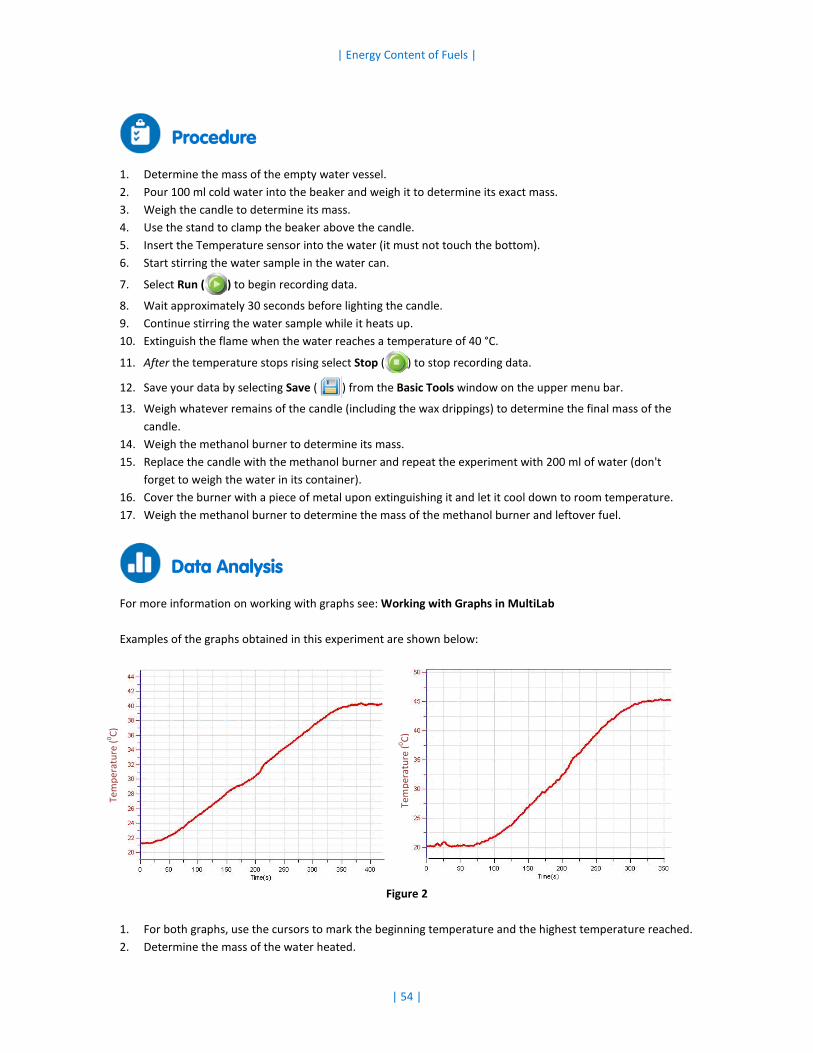
For more information on working with graphs see: Working with Graphs in MultiLab Examples of the graphs obtained in this experiment are shown below:
Figure 2
1. For both graphs, use the cursors to mark the beginning temperature and the highest temperature reached. 2. Determine the mass of the water heated.
Tem
pera
ture
(0 C)
Tem
pera
ture
(0 C)

| Energy Content of Fuels |
| 55 |
3. How much did the temperature of the water change (∆T)? 4. Calculate the heat (Q) absorbed by the water according to equation 1 5. Determine the masses of the burnt paraffin and the methanol. 6. Calculate the %-efficiency for both experiments. Divide your experimental value [kJ/g] by the appropriate
literature values and multiply the answer by 100. The literature values are 41.5 kJ/g (paraffin) and 30.0 kJ/g (ethanol).
Questions
1. Which fuel produces more energy per gram burned? Give an explanation for the difference (hint: methanol CH3OH is an oxygenated molecule, paraffin C25H52 does not contain oxygen).
2. Suggest some advantages of using ethanol (or paraffin) as a fuel. 3. Discuss the heat loss factors contributing to the inefficiency of the experiment.

| 56 |
Chapter 12
Boyle’s Law
Figure 1
Introduction
Boyle’s law states that at constant temperature, the pressure of a given mass of a dry gas is inversely proportional to its volume:
𝑃 =𝑘𝑉
(1)
Where:
P = The pressure. k = A constant. V = The volume of the gas. The magnitude of the constant depends on the temperature, the mass and the nature of the gas. In this experiment we will change the volume of air in a syringe and measure the pressure with the Pressure sensor connected directly to the syringe.

| Boyle’s Law |
| 57 |
Equipment
• einstein™ LabMate and a computer with MultiLab
• Pressure sensor (150 to 1150 mbar)
• Syringe (50 ml)
Equipment Setup Procedure
1. Launch MultiLab ( ).
2. Connect the Pressure sensor to one of the ports on the einstein™ LabMate. 3. In the Current Setup Summary window choose Full Setup and use the table below to set up the
experiment. Make sure that only the Pressure sensor is selected under Measurements.
Current Setup Summary
Program the sensor to log data according to the following setup:
Sensor: Pressure (150 to 1150 mbar)
Measurements: Pressure (mbar)
Sampling: Manual
Samples: 50
Note: Ensure that only the external Pressure sensor (150 – 1150 mbar) is selected and not the internal Pressure sensor (0 – 400 kPa).
Procedure
1. Pull out the syringe’s plunger to the 50 ml mark in order to fill the syringe with air. 2. Connect the Pressure sensor directly to the syringe’s nozzle (see Figure 1).
3. Select Run ( ) to enable recording data.
4. Collect the data manually: Select Manual Sampling ( ) each time you wish to record a data sample.
5. Make your first measurement by selecting Manual Sampling ( ).
6. Begin to push the syringe plunger inward, decreasing the volume of air inside to 45 ml, then select Manual
Sampling ( ) to make a measurement.
7. Repeat step 6 for syringe volumes of 40 ml, 35 ml, 30 ml, 25 ml and 20 ml.
8. Select Stop ( ) to stop collecting data.

| Boyle’s Law |
| 58 |
Data Analysis
For more information on working with graphs see: Working with Graphs in MultiLab 1. You now need to export the data so that you can enter the volume corresponding to each measurement
into your data table. Select Export ( ) to save the data as a csv file.
2. Open the exported data in a suitable spreadsheet or graphing program. 3. Add a column to the data and enter the volume corresponding to each measurement of pressure (see an
example in Figure 2 below).
Figure 2
4. Create a new column in which you will calculate the reciprocal of the volume. 5. Calculate the reciprocal of the volume (1/V) for each measurement. 6. Create a graph of Pressure vs. 1/Volume.
Questions
1. Is the relationship between Pressure and Volume direct or inverse? Explain.
2. Can you infer from your graph what the gas pressure will be if the volume is reduced to 10 mL?

| 59 |
Chapter 13
Effects of Variations in Air Temperature on Air Pressure: The Combined Gas Law
Figure 1
Introduction
The volume of gases, V, is affected by their temperature, T. As stated by Charles' Law, a sample of gas at a fixed pressure increases in volume linearly with temperature:
𝑉 ∝ 𝑇 (1)
𝑉𝑇
= 𝑐𝑜𝑛𝑠𝑡𝑎𝑛𝑡 (2)
Charles' Law combined with Boyle’s Law can be expressed in one statement - The Combined Gas Law. This law states that the volume occupied by a given amount of gas is proportional to the absolute temperature divided by the pressure, P:
𝑃𝑉𝑇
= 𝑐𝑜𝑛𝑠𝑡𝑎𝑛𝑡 (2)
In this experiment we investigate the relationship between pressure and temperature and their effect on gas behavior, by measuring the effect of warming a constant volume of air trapped in a sealed flask on its pressure.

| Effects of Variations in Air Temperature on Air Pressure: The Combined Gas Law |
| 60 |
Equipment
• einstein™ LabMate and a computer with MultiLab • Pressure sensor (150 – 1150 mbar) • Temperature sensor (-40 °C to 140 °C) • 50 ml glass flask • Rubber cork • 20-gauge syringe needles • Three-way valve • Stand • Magnetic stirrer/hot plate and stir bar • Safety goggles
Equipment Setup Procedure
1. Launch MultiLab ( ).
2. Connect the Pressure sensor to one of the ports on the einstein™ LabMate. 3. Connect the Temperature sensor to one of the ports on the einstein™ LabMate. 4. Assemble the equipment as illustrated in Figure 2 below. 5. A syringe needle (20-gauge) is inserted through the cork, until its tip projects slightly out of the cork
(Figure 1). 6. At the other end of the needle, projecting out of the upper side of the cork, attach a three-way valve.
Attach a Pressure sensor to the other end of the valve. 7. Turn the valve until its opening is directed horizontally. In this position, air can flow through the valve from
the flask to the surroundings. 8. In the Current Setup Summary window choose Full Setup and use the table below to set up the
experiment. Make sure that only the Pressure and Temperature sensors are selected under Measurements.
Current Setup Summary
Program the sensors to log data according to the following setup:
Sensor: Pressure 150 - 1150 mbar
Measurements: Pressure (mbar)
Sensor: Temperature (-40 °C – 140 °C)
Measurements: Temperature (°C)
Rate: Every second
Samples: 500
Duration: 8 minutes 20 seconds

| Effects of Variations in Air Temperature on Air Pressure: The Combined Gas Law |
| 61 |
Note: Ensure that only the external Pressure sensor (150– 1150 mbar) and the Temperature sensor (-40 °C – 140 °C) are selected and not the internal Pressure sensor (0– 400 kPa) or internal Temperature sensor (-30 °C – 50 °C).
Procedure
1. Assemble the equipment as illustrated in Figure 1 above. 2. Put on the safety goggles. 3. Pierce a hole in the cork, big enough to insert the tip of the Temperature sensor.
Alternatively, make a narrow slit on the side of the cork. 4. Place the magnetic stir bar in the flask. 5. Fill the glass flask with water. Leave a small volume of air in the flask, to prevent water from
reaching the needles. 6. Insert the Temperature sensor into the hole or the slit prepared in the cork. 7. Cork the flask and start stirring 8. Make sure the pressure in the flask equals atmospheric pressure (around 1000 mbar) then turn the valve
to prevent air entering the flask.
9. Select Run ( ) to begin recording data.
10. Follow the pressure level in the Graph window of MultiLab. 11. Start warming the flask. Turn the warming button of the magnetic stirrer/hot plate to a middle position.
Follow changes in pressure for about 5 minutes.
12. Select Stop ( ) to stop collecting data.
13. Save your data by selecting Save ( ) from the Basic Tools window on the upper menu bar.

| Effects of Variations in Air Temperature on Air Pressure: The Combined Gas Law |
| 62 |
Data Analysis
For more information on working with graphs see: Working with Graphs in MultiLab 1. Compare the pattern of changes in the pressure with that of temperature: Did you find any similarity
between the two of them? An example of the original graphs obtained in this experiment is shown below:
Figure 2
2. Find the correlation between the changes in temperature and pressure by displaying a graph of Pressure
vs. Temperature. Create a graph of pressure vs. temperature by selecting the down arrow from the Graph toolbar and choosing Temperature as your x-axis measure (Figure 4).
Pressure
Temperature
Tem
pera
ture
(0 C) Pressure (m
bar)
1350
1300
1250
1200
1150
1100
1000
950
900
850
800

| Effects of Variations in Air Temperature on Air Pressure: The Combined Gas Law |
| 63 |
An example of the Pressure vs. Temperature obtained in this experiment is shown below:
Figure 3
Questions
1. Changes in temperature and in pressure displayed a non-linear curve. Why? 2. What would be the shape of the curves if the flask was warmed in a bath? 3. How are the pressure changes during the experiment related to the changes in temperature?
Relate to the Pressure vs. Temperature graph. 4. What would be the effect of cooling the flask on the pressure? 5. Suppose that the water volume in the flask was reduced. What would be the effect of warming the flask
compared to the results in the present experiment?
Further Suggestions
1. Warm the flask for a while. Then, stop warming the flask. As the temperature stabilizes, start cooling the flask. Follow the changes in pressure measured in the flask
2. Perform the experiment with different water volumes in the flask. Compare the effect of warming or cooling on the pressure in each instance.
Pres
sure
(mba
r)

| 64 |
Chapter 14
Saltwater Conductivity
Figure 1
Introduction
Dissolving solid sodium chloride in water releases ions according to the following equation:
NaCl(s) ⟶ Na(aq)+ + Cl(aq)
− (1)
In this experiment we will study the effect of increasing sodium chloride concentration on conductivity. We will be measuring conductivity as the ion concentration of the solution being monitored is gradually being increased by the addition of concentrated NaCl drops.
Equipment
• einstein™ LabMate and a computer with MultiLab
• Conductivity sensor (0-20 mS)
• 200 ml distilled water
• 250 ml glass flask
• 50 ml sodium chloride solution
• Magnetic stirrer and stir bar
• Safety goggles

| Saltwater Conductivity |
| 65 |
Equipment Setup Procedure
1. Launch MultiLab ( ).
2. Connect the Conductivity sensor to one of the ports on the einstein™ LabMate. 3. Assemble the equipment as illustrated in Figure 1. 4. In the Current Setup Summary window choose Full Setup and use the table below to set up the
experiment. Make sure that only the Conductivity sensor is selected under Measurements.
Current Setup Summary
Program the sensor to log data according to the following setup:
Sensor: Conductivity (0 – 20 mS)
Measurements: Conductivity (mS)
Sampling: Manual
Samples: 20
Procedure
Always wear safety goggles. 1. Place the magnetic stir bar in the flask. 2. Pour 40 ml of distilled water into the flask and place it on the magnetic stirrer. 3. Insert the Conductivity electrode into the flask. 4. Start stirring the water in the flask.
5. Select Run ( ) to enable recording the conductivity of the solution in the flask.
6. Collect the data manually: Select Manual Sampling ( ) on the main toolbar each time you wish to
record a data sample.
7. Add one drop of sodium chloride solution to the distilled water. Stir to ensure thorough mixing. 8. Select Manual Sampling ( ) to measure the conductivity of the solution in the flask.
9. Repeat this process 9 times until you have added a total of 10 drops to the water. 10. Change the rate of stirring during the experiment and follow its effect on the rate of change in
conductance.
11. Save your data by selecting Save ( ) from the Basic Tools window on the upper menu bar.
Data Analysis
For more information on working with graphs see: Working with Graphs in MultiLab 1. Calculate the rate of change in conductance obtained in the process:
a. Select the plot line on the graph b. Select Curve fit ( ) from the Analysis window on the upper menu bar.

| Saltwater Conductivity |
| 66 |
c. In the Curve fit window which opens, choose Linear from the Curve fit drop down menu. d. The fit equation will be displayed next to the second cursor.
2. The slope of the fit line is the rate of change in conductance An example of the graph of conductivity and conductance changes obtained in this experiment is shown below. The straight line is the linear fit.
Figure 2
Questions
1. Describe the change in conductivity as the concentration of NaCl solution was increased. 2. What kind of mathematical relationship does there appear to be between conductivity and concentration?
Further Suggestions
1. Add a solution of CaCl2 (with the same concentration) in place of NaCl. 2. Try this experiment again but change the stirring rate. What is the effect on conductivity?
Explain this phenomenon.
Cond
uctiv
ity (m
S)

| 67 |
Chapter 15
The Lambert-Beer Law
Figure 1
Introduction
The amount of light penetrating a solution is known as transmittance, expressed as the ratio between the initial light intensity I0 and the intensity of the transmitted light, It, :
𝑇 =𝐼𝑡𝐼o
(1)
Where: T = Transmittance. It = Intensity of the transmitted light. I0 = Intensity of the initial light beam. Even though one might think the relationship between transmittance and absorbance would be a simple inverse relationship, the true relationship between these two variables is inverse and logarithmic (base 10):
𝐴 = log1𝑇
= − log𝑇 (2)
Where:

| The Lambert-Beer Law |
| 68 |
A = Absorption.
T = Transmittance as a number between 0 and 1, 𝑇%100
The Lambert-Beer Law defines the relationship between absorbance and concentration. The absorbance of a dissolved substance is a linear function of its concentration. The length of the light path (thickness of the cuvettes) and the extinction coefficient (a substance specific constant) determine the slope of the linear plot.
𝐴 = ε𝑑𝑐 (3)
Where:
ε = Extinction coefficient. d = Path length (width of the cuvette). c = Concentration. The Lambert-Beer Law, however, is valid only for dilute solutions. The limits for its validity differ for different materials. As a general rule, every material showing absorption of up to 0.5 - 0.6 still obeys the Lambert-Beer Law. In this experiment we observe the linear increase of absorbance of a CuSO4 solution with increasing concentrations. This will allow us to determine its extinction coefficient at a given wavelength within its absorption spectrum.
Equipment
• einstein™ LabMate and a computer with MultiLab
• Colorimeter sensor
• Four CuSO4·5 H2O solutions ranging from 0.006 to 0.05 mol/L
Equipment Setup Procedure
1. Launch MultiLab ( ).
2. Connect the Colorimeter sensor to one of the ports on the einstein™ LabMate. 3. In the Current Setup Summary window choose Full Setup and use the table below to set up the
experiment. Make sure that only the Colorimeter sensor is selected under Measurements.
Current Setup Summary
Program the sensor to log data according to the following setup:
Sensor: Colorimeter 0-100%
Measurements: Absorbance(%)
Sampling: Manual
Samples: 10

| The Lambert-Beer Law |
| 69 |
Procedure
1. Insert the red filter slide into the Colorimeter. 2. Calibrate the Colorimeter sensor (see the Colorimeter datasheet).
3. Select Run ( ) to enable recording data.
4. Measure your samples in order of increasing concentration. Collect the data manually: Select Manual
Sampling ( ) on the main toolbar each time you wish to record a data sample.
5. Select Stop ( ) to stop collecting data.
6. Save your data by selecting Save ( ) from the Basic Tools window on the upper menu bar.
An example of the graph obtained in this experiment is shown below:
Figure 2
Data Analysis
For more information on working with graphs see: Working with Graphs in MultiLab 1. Note that the Colorimeter measured transmission. Now this must be converted into absorption:
a. Use the cursor to select the plot line. b. Select Math functions ( ) from the Analysis window on the upper menu bar.
In the Math function window which opens, choose Log10 from the Function drop down menu. In the A text box enter -1. In the B text box enter 0.01. In the Name text box enter a name (e.g. Absorption).
2. You now need to export the data so that you can enter the CuSO4 concentration. Select Export ( ) from
the Graph toolbar to save the data as a csv file. 3. Open the exported data in a suitable spreadsheet or graphing program.
Tran
smitt
ance
(%)

| The Lambert-Beer Law |
| 70 |
4. Add a new column to the data table. a. If possible, give the new column a name (e.g. Concentration) and indicate the units (e.g. mol/L). b. In the table, enter the concentrations of the samples.
5. Create a graph of Absorption vs. Concentration in your spreadsheet or graphing program. A sample graph is shown in Figure 3 below.
Figure 3
6. Apply a linear fit to obtain the extinction coefficient of CuSO4 7. Divide the slope by the path length (width of the cuvette) to obtain the extinction coefficient of CuSO4.
Abso
rban
ce

| 71 |
Chapter 16
Exploring a Flame
Figure 1
Introduction
A flame does not have a uniform temperature. Temperature differences within a flame can be mapped with a thermocouple (a highly sensitive, fast responding Temperature sensor ranging from 0 °C to well over 1000 °C). In the following experiment, we are going to explore a candle flame in three characteristic areas labeled 1, 2 and 3 in Figure 1.
Equipment
• einstein™ LabMate and a computer with MultiLab
• Temperature sensor TC-K (0 °C to 1200 °C)
• Candle
• Matches
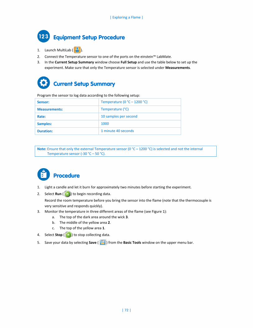
| Exploring a Flame |
| 72 |
Equipment Setup Procedure
1. Launch MultiLab ( ).
2. Connect the Temperature sensor to one of the ports on the einstein™ LabMate. 3. In the Current Setup Summary window choose Full Setup and use the table below to set up the
experiment. Make sure that only the Temperature sensor is selected under Measurements.
Current Setup Summary
Program the sensor to log data according to the following setup:
Sensor: Temperature (0 °C – 1200 °C)
Measurements: Temperature (°C)
Rate: 10 samples per second
Samples: 1000
Duration: 1 minute 40 seconds
Note: Ensure that only the external Temperature sensor (0 °C – 1200 °C) is selected and not the internal Temperature sensor (-30 °C – 50 °C).
Procedure
1. Light a candle and let it burn for approximately two minutes before starting the experiment.
2. Select Run ( ) to begin recording data.
Record the room temperature before you bring the sensor into the flame (note that the thermocouple is very sensitive and responds quickly).
3. Monitor the temperature in three different areas of the flame (see Figure 1): a. The top of the dark area around the wick 3. b. The middle of the yellow area 2. c. The top of the yellow area 1.
4. Select Stop ( ) to stop collecting data.
5. Save your data by selecting Save ( ) from the Basic Tools window on the upper menu bar.

| Exploring a Flame |
| 73 |
Data Analysis
For more information on working with graphs see: Working with Graphs in MultiLab The plot of Temperature vs. Time shows us that the flame is hottest at the top and gets cooler the lower you dip the sensor:
Figure 2
Questions
1. What are the temperatures in each of the flame zones? (1, 2 & 3). 2. Why do you think the hottest part of the flame is at the top?
Tem
pera
ture
(0 C)
1
2 3

| 74 |
Chapter 17
Freezing and Melting of Water
Figure 1
Introduction
Freezing is the process of matter changing from the liquid state to the solid state. Melting is the process of solids changing to liquids. These phase transitions occur at the freezing or melting temperature respectively. In this experiment we investigate the freezing and melting temperature of water.
Equipment
• einstein™ LabMate and a computer with MultiLab
• Temperature sensor (-40 °C to 140 °C)
• Stand with utility clamp
• Graduated cylinder
• Beaker (250 ml)
• Test tube
• Stirring rod
• Water
• Ice cubes
• Salt

| Freezing and Melting of Water |
| 75 |
Equipment Setup Procedure
1. Launch MultiLab ( ).
2. Connect the Temperature sensor to one of the ports on the einstein™ LabMate. 3. Assemble the equipment as illustrated in Figure 1. 4. In the Current Setup Summary window choose Full Setup and use the table below to set up the
experiment. Make sure that only the Temperature sensor is selected under Measurements.
Current Setup Summary
Program the sensor to log data according to the following setup:
Sensor: Temperature (-40 °C – 140 °C)
Measurements: Temperature (°C)
Rate: Every 10 seconds
Samples: 200
Duration: 33 minutes 20 seconds
Note: Ensure that only the external Temperature sensor (-40 °C – 140 °C) is selected and not the internal Temperature sensor (-30 °C – 50 °C).
Procedure (Part I, Freezing)
1. Pour at least 150 ml of ice cubes and cold water into a 250 ml beaker. 2. Put 1 ml of water into a 5 ml test tube and fix it to the stand with a clamp. Lower the test tube into the
beaker of ice water. You have to adjust the test tube so that the sample is below the ice water level. 3. Place a Temperature sensor into the water inside the test tube.
4. Select Run ( ) to begin recording data.
5. Add about five spoons of salt to the beaker and stir with a glass stirring rod.
6. After about 15 minutes select Stop ( ) to stop recording while keeping the test tube in the ice-water
bath.
7. Save your data by selecting Save ( ) from the Basic Tools window on the upper menu bar.
Procedure (Part II, Melting)
1. Select Run ( ) to start recording data again, raise the test tube and fix it in a position above the ice-
water bath. Dispose of the ice water and add 150 ml warm tap water to the beaker. Lower the test tube into the warm water.
2. After another 15 minutes select Stop ( ) on the upper tool bar to stop recording data.
3. Save your data by selecting Save ( ) from the Basic Tools window on the upper menu bar.

| Freezing and Melting of Water |
| 76 |
Data Analysis
For more information on working with graphs see: Working with Graphs in MultiLab Examples of the graphs obtained in the experiments are shown below:
Part I: Freezing water Part II: Melting the frozen water
1. What happened to the water temperature during the freezing stage and during the melting stage? 2. What is the freezing point and the melting point of the water? 3. How does the freezing point of water compare to the melting point? 4. How does the kinetic energy of the water within the test tube change during the melting and freezing
processes? Does it increase, decrease or remain the same, when: a. The temperature changes at the beginning and the end of Part I. b. The temperature remains constant in Part I. c. The temperature changes at the beginning and the end of Part II. d. The temperature remains constant in Part II.
5. Did the potential energy increase or decrease in those parts of Question 4 where kinetic energy remained constant?
Tem
pera
ture
(0 C)
Tem
pera
ture
(0 C)

| 77 |
Chapter 18
Another Look at Freezing Temperature
Figure 1
Introduction
In Experiment 17: Freezing and Melting of Water, we saw that the temperature of pure water remains constant at its freezing temperature during the freezing and melting process. Now we are going to observe the freezing process of phenyl salicylate. Furthermore, we will observe the effect on the freezing point, when a small amount of another substance (e.g. benzoic acid) is dissolved in the phenyl salicylate.
Equipment
• einstein™ LabMate and a computer with MultiLab
• Three Temperature sensors (-40 °C to 140 °C)
• 1 liter (or larger) beaker
• Test tube with 2 g phenyl salicylate
• Test tube with 2 g phenyl salicylate and a few milligrams of benzoic acid
• Stirring rod

| Another Look at Freezing Temperature |
| 78 |
Equipment Setup Procedure
1. Launch MultiLab ( ).
2. Connect the Temperature sensors to ports on the einstein™ LabMate. 3. Assemble the equipment as illustrated in Figure 1. 4. In the Current Setup Summary window choose Full Setup and use the table below to set up the
experiment. Make sure that only the Temperature sensors are selected under Measurements.
Current Setup Summary
Program the sensors to log data according to the following setup:
Sensor: Temperature (-40 °C – 140 °C)
Measurements: Temperature (°C)
Sensor: Temperature (-40 °C – 140 °C)
Measurements: Temperature (°C)
Sensor: Temperature (-40 °C – 140 °C)
Measurements: Temperature (°C)
Rate: Every second
Samples: 1000
Duration: 16 minutes 40 seconds
Note: Ensure that only the external Temperature sensors (-40 °C – 140 °C) are selected and not the internal Temperature sensor (-30 °C – 50 °C).
Procedure
1. Pour about 1 L of water into a beaker. The water should be at about 30 °C. Insert one of the Temperature sensors into this beaker to monitor the water temperature.
2. To melt your samples, prepare a second beaker with hot water (60 to 80 °C). 3. Place the two sample test tubes into the hot water until you see a clear liquid in both test tubes. 4. Place a Temperature sensor in each sample test tube and move them quickly to the beaker containing the
30 °C water.
5. Select Run ( ) to begin recording data.
6. Stir your samples slightly as long as they are melted. 7. Pay attention to the test tubes, as the clear liquid will soon contain increasing amounts of white
precipitates, until the liquid is completely frozen.
8. Save your data by selecting Save ( ) from the Basic Tools window on the upper menu bar.

| Another Look at Freezing Temperature |
| 79 |
Data Analysis
For more information on working with graphs see: Working with Graphs in MultiLab 1. What was the freezing point of pure phenyl salicylate according to your data? 2. What was the freezing point of the benzoic acid-phenyl salicylate mixture?
An example of the graph obtained in this experiment is shown below:
Figure 2
Questions
1. Based on this experiment and its result, what method could a chemist use to check whether or not an unknown liquid is pure?
2. Why does the freezing point change by dissolving another component in phenyl salicylic acid? 3. Does the nature of this change depend on the freezing point of the dissolved compound?
Freezing temperature of pure phenyl salicylate
Freezing temperature of benzoic acid-phenyl salicylate mixture
Tem
pera
ture
(0 C)

| 80 |
Chapter 19
Chemical Equilibrium: Finding a Constant, Kc
Figure 1
Introduction
One may believe that chemical reactions completely convert the initial compounds (reactants) into products. However, there are a large number of reactions resulting in a mixture of reactants and products. One example is the reaction of iron(III) ions (Fe3+) with thiocyanate ions (SCN-) forming thiocyanoiron(III) ions (FeSCN2+):
Fe(aq)3+ + SCN(aq)
− ⇌ FeSCN(aq)2+ (1)
The reactants and products in this equation are said to be in equilibrium with each other. The equilibrium constant, Kc, is a measure for the quantity of a product formed relative to the amount of the reactants still remaining (see equation 2). This means that the higher the Kc, the more product is formed. If Kc is 1, the reactant and product concentrations are similar. To determine Kc, you have to first determine the equilibrium concentrations of all the components.
Kc =[FeSCN2+]eq
[Fe3+]eq[SCN−]eq (2)
In this experiment we will use the Colorimeter sensor to determine the concentration of the reaction product. As FeSCN2+ absorbs blue light (and therefore appears as red in solution), we are going to use the blue slide of

| Chemical Equilibrium: Finding a Constant, Kc|
| 81 |
the Colorimeter sensor to determine its concentration in four samples compared to a standard solution with a known concentration of FeSCN2+. The Fe3+ concentration in this standard solution must be about 100 times higher than that of the test solutions. This high concentration, along with the low initial concentration of KSCN, forces the equilibrium far to the right, ensuring that all the SCN- ions have reacted with Fe3+ to form FeSCN2+.
Remember that the absorption of FeSCN2+ depends linearly on the concentration according to Lambert-Beer’s
Law. From the determined concentrations, we are then able to calculate the concentrations of the other components (see Data Analysis below).
Equipment
• einstein™ LabMate and a computer with MultiLab
• Colorimeter sensor
• Plastic cuvettes
• Test tubes
• Stirring rod
• Thermometer
• Scale
• 0.002 M KSCN
• 0.002 M Fe(NO3)3 in 1 M HNO3
• 0.2 M Fe(NO3)3 in 1 M HNO3 (standard solution)
• Pipettes
• Three 100 ml beakers
• Safety goggles and gloves
Attention! Fe(NO3)3 solutions are prepared from 1 M HNO3. Handle them with great care.
Equipment Setup Procedure
Always wear safety goggles and gloves. 1. Prepare four test tubes of a minimum capacity of 10 ml. Label them 1-4. 2. Pour about 30 ml of 0.002 M Fe(NO3)3 solution into a 100 ml beaker and transfer five ml of it into each of
the labeled test tubes. 3. Pour about 25 ml of the 0.002 M KSCN solution into another 100 ml beaker and transfer 2, 3, 4 and 5 ml of
this solution into test tubes 1 to 4 according to the table below. 4. Dilute each solution in the four test tubes with water according to the table below. Mix each solution
thoroughly with the glass stirring rod. Make sure that you wash and dry the rod each time before dipping it into the next solution.

| Chemical Equilibrium: Finding a Constant, Kc|
| 82 |
5. Launch MultiLab ( ).
6. Connect the Colorimeter sensor to one of the ports on the einstein™ LabMate. 7. Measure and record the temperature of one of the prepared solutions as the determined Kc depends on
the temperature. 8. Prepare the standard solution of FeSCN2+ by transferring 9 ml of 0.2 M Fe(NO3)3 into a fifth test tube
(labeled 5). Transfer 1 ml of 0.002 M KSCN into the same test tube. Stir thoroughly. 9. In the Current Setup Summary window choose Full Setup and use the table below to set up the
experiment. Make sure that only the Colorimeter sensor is selected under Measurements.
Current Setup Summary
Program the sensor to log data according to the following setup:
Sensor: Colorimeter 0-100%
Measurements: Absorbance (%)
Sampling: Manual
Samples: 10
Procedure
1. Insert the blue filter slide into the Colorimeter. 2. Calibrate the Colorimeter (refer to the Colorimeter sensor sheet).
3. Select Run ( ) to enable recording data.
4. Measure your samples and the reference sample. Collect the data manually. Select Manual Sampling
( ) on the main toolbar each time you wish to record a data sample. Note that you initially measure
transmission (%T).
5. Select Stop ( ) to stop collecting data.
6. Save your data by selecting Save ( ) from the Basic Tools window on the upper menu bar.
7. Determine the corresponding absorption (A) from the measured transmission as explained in Experiment 15: The Lambert Beer Law.
Test Tube 0.002 M Fe(NO3)3 (ml) 0.002 M KSCN (ml) H2O (ml)
1 5 2 3
2 5 3 2
3 5 4 1
4 5 5 0

| Chemical Equilibrium: Finding a Constant, Kc|
| 83 |
Data Analysis
For more information on working with graphs see: Working with Graphs in MultiLab 1. Prepare a table to write down the results for the calculations below for each of the four experiments. 2. First, calculate the initial concentrations of Fe3+ and SCN- in each test tube, based on composition and
dilution with water. Refer to step 2 of the Equipment Setup Procedure for the volume of each component used in test tubes 1-4. Note that you need to know the initial concentrations to proceed with calculating the equilibrium concentrations. The initial concentration of iron(III), [Fe3+]i, in each test tube can be calculated from the volumes and concentrations used, as follows:
[Fe3+]i =VFe(NO3)3
Vtotal× 0.002 M (3)
[Fe3+]i must be the same for all the four test tubes, as you always added the same volume of 0.002 M Fe(NO3)3 solution.
Similarly, the inital concentration of thiocyanate, [SCN-]i,in each test tube can be calculated:
[SCN−]i =VKSCNVtotal
× 0.002 M (4)
3. Compare the absorption values of your four "unknown" solutions to the absorption value from your "known" reference standard to calculate the equilibrium concentrations of thiocyanoiron(III) ion ([FeSCN2+]eq) as follows: (Here we assume that because of its relatively low concentration, all of the initial thiocyanate ion has reacted to form thiocyanoiron(III) ion and so, [FeSCN2+]std = [SCN-]i = 0.002M)
[FeSCN2+]eq =Aeq
Astd× [FeSCN2+]std (5)
Where:
Aeq = The absorbance of the "unknown" solution in equilibrium. Astd= The absorbance of the "known" standard reference solution.
4. Calculate the equilibrium concentration for Fe3+ and SCN- ([Fe3+]eq and [SCN-]eq).
[Fe3+]eq = [Fe3+]i − [FeSCN2+]eq (6)
[SCN−]eq = [SCN−]i − [FeSCN2+]eq (7)
5. Calculate Kc from equation 2 above (see Introduction) for each test tube:
Kc =[FeSCN2+]eq
[Fe3+]eq[SCN−]eq (2)

| Chemical Equilibrium: Finding a Constant, Kc|
| 84 |
6. Determine an average value for Kc. How constant were your values? An example of the Absorption vs. Test Tube graph obtained in this experiment is shown below:
Figure 2
Questions
1. What does Kc express? 2. What happens to Kc, if you add an additional aliquot or portion of one of the reactants (Fe3+ or SCN-)? 3. Why do you have to prepare the Fe(NO3)3 solutions in 1M HNO3 instead of water? 4. The standard concentration of [FeSCN2+] is known in this experiment. You could calculate it also from the
measured absorption of the standard solution (test tube 5). What additional information would you need in order to calculate it?
Abso
rptio
n

imagine • explore • learnwww.einsteinworld.com
ALBERT EINSTEIN and EINSTEIN are either trademarks or registered trademarks of The Hebrew University of Jerusalem. Represented exclusively by GreenLight. Official licensed merchandise. Website: einstein.biz © 2014 Fourier Systems Ltd. All rights reserved. Fourier Systems Ltd. logos and all other Fourier product or service names are registered trademarks or trademarks of Fourier Systems. All other registered trademarks or trademarks belong to their respective companies. einstein™World LabMate, einstein™Activity Maker, MultiLab, MiLAB and Terra Nova, are registered trademarks or trademarks of Fourier Systems LTD. First Edition, April 2014.
www.einsteinworld.com
USA8940 W. 192nd St.
Unit IMokenaIL 60448
Tel: (877) 266-4066
www.FourierEdu.com
Israel 16 Hamelacha St.POB 11681Rosh Ha’ayin 48091Tel: +972-3-901-4849 Fax: +972-3-901-4999
Experiments in C
hemistry for M
ultiLab
Experiments in Chemistry for MultiLab™