Embed Size (px)
Citation preview
Experimental Investigation of
Laser-Induced Optoacoustic Wave Propagation for Damage Detection
by
Venkateshwaran Ravi Narayanan
A Thesis Presented in Partial Fulfillment
of the Requirements for the Degree
Master of Science
Approved July 2019 by the
Graduate Supervisory Committee:
Yongming Liu, Chair
Houlong Zhuang
Qiong Nian
ARIZONA STATE UNIVERSITY
August 2019
brought to you by COREView metadata, citation and similar papers at core.ac.uk
provided by ASU Digital Repository
i
ABSTRACT
This thesis intends to cover the experimental investigation of the propagation of laser-
generated optoacoustic waves in structural materials and how they can be utilized for
damage detection. Firstly, a system for scanning a rectangular patch on the sample is
designed. This is achieved with the help of xy stages which are connected to the laser
head and allow it to move on a plane. Next, a parametric study was designed to determine
the optimum testing parameters of the laser. The parameters so selected were then used in
a series of tests which helped in discerning how the Ultrasound Waves behave when
damage is induced in the sample (in the form of addition of masses). The first test was of
increasing the mases in the sample. The second test was a scan of a rectangular area of
the sample with and without damage to find the effect of the added masses. Finally, the
data collected in such a manner is processed with the help of the Hilbert-Huang transform
to determine the time of arrival. The major benefits from this study are the fact that this is
a Non-Destructive imaging technique and thus can be used as a new method for detection
of defects and is fairly cheap as well.

ii
ACKNOWLEDGMENTS
I would like to acknowledge Dr. Liu for helping me in progressing through my research
work on this thesis and for teaching my many things along the way.
My fellow lab members who helped through the various stages of this work.
My family for being there for me emotionally.

iii
TABLE OF CONTENTS
Page
LIST OF TABLES ................................................................................................................... iv
LIST OF FIGURES .................................................................................................................. v
CHAPTER
1 INTRODUCTION ................................................................................................ 1
Background of Wave Based NDE .......................................................................... 1
Motivation and Objective ........................................................................................ 2
Major Work.............................................................................................................. 3
2 EXPERIMENTAL SETUP .................................................................................. 4
Principle of Laser Scanning .................................................................................... 5
Tests Conducted....................................................................................................... 6
Difficulties In Testing ............................................................................................ 13
3 DATA PROCESSING AND RESULTS ............................................................ 14
Data Processing ..................................................................................................... 14
Results .................................................................................................................... 16
4 CONCLUSION AND FUTURE WORK............................................................ 33
REFERENCES ...................................................................................................................... 36
APPENDIX A ........................................................................................................................ 38
APPENDIX B ........................................................................................................................ 40

iv
LIST OF TABLES
Table Page
1- Results of the parametric Test ...................................................................................... 17
2 - Results of Test 2 .......................................................................................................... 20
3- Time of Arrival data for Test 3 ..................................................................................... 22
4- Time of Arrival for data for test 4 ................................................................................ 24
5 Time of Arrival data for Test 5 ...................................................................................... 28
6 Points Detected by the different Criterion .................................................................... 30

v
LIST OF FIGURES
Figure Page
1 – Connection of Components........................................................................................... 5
2- Experimental Setup......................................................................................................... 6
3- Aluminum Sample .......................................................................................................... 7
4 - Path of the laser ............................................................................................................. 8
5 - Position of the points where the laser would be fired for scanning ............................... 9
6 - Position of the added masses ....................................................................................... 10
7 - Position of the added masses ....................................................................................... 11
8 - Position of the added masses ....................................................................................... 12
9 - Data without any Filtering ........................................................................................... 15
10 Data after filtering in the oscilloscope ......................................................................... 15
11 Signal data after Empirical Modal Decomposition ...................................................... 16
12 - No signal Received .................................................................................................... 18
13- Signal Barely Received .............................................................................................. 19
14 - Signal is clearly Received.......................................................................................... 19
15 - Plot of No. of Magnets v/s TOF ................................................................................ 21
16 - Plot of Time of Arrival v/s Distance from Sensor ..................................................... 23
17 - Testing Area .............................................................................................................. 26
18 - Plot of Tof with respect to relative position of each point ........................................ 26
19 - Isometric view of the previous plot .......................................................................... 27
20 - Location of added masses for dense Scan ................................................................. 31
21 - Dense Scan Top view of ToF .................................................................................... 31

vi
Figure 22Dense Scan ToF Isometric View of Plot ........................................................... 32
1
CHAPTER 1
INTRODUCTION
Defects of different kind exist in all the materials around us. They vary from being easily
discernible by visual inspection, (outer cracks, scratched surfaces etc.) to micro defects like
voids which require special techniques for detecting them. There are different methods to
determine the extent of these defects and they vary depending on the application of the
material. Depending on the situation, the traditional nondestructive testing methods might
not be feasible. For instance, if the situation calls for determining defects in aircrafts, ships,
heavy machinery, etc. attaching sensors for testing might not be feasible due to regulations,
cost, type of defect etc.
A good solution for such concerns might be found in non-contact nondestructive evaluation
(NDE) methods. Damage detection due to propagation of Laser induced Lamb waves is
such a method which is feasible and is something which is well documented. This project
tries to develop a novel NDE method for using the Lamb waves induced by a Pulsed Laser.
The laser is used to generate the Lamb waves in a raster scan pattern and said waves are
detected by piezoelectric sensors and then processed.
1.1 Background of wave based NDE methods
Wave based nondestructive evaluation methods are of several types. Some of the most
commonly used ones are where sensors are glued/attached to the surface of the sample for
generation of and receiving the wave signal [1]. This method is generally not feasible for
large machines are aircrafts as it would involve the usage of a large network of sensors for
damage detection which would be complex to implement as well as would have the
2
drawback being inefficient cost wise. Traditionally, this method involves gluing the
necessary sensors on the sample [2] which might cause damage on its own which further
adds to the drawback of this method. A second method involves sensor actuators at the
excitation terminal (such as a piezoelectric transducer) but laser based receiver terminal
(such as a laser vibrometer). The excitation terminal can be replaced with a laser terminal
as well making the entire process entirely non-contact based [5]. In this method, the laser
causes localized heating due to being incident on the sample. Since the material
surrounding the one incident spot is cooler, the material is not able to expand which causes
a stress wave being generated. This ultrasonic wave would then be detected by the laser
vibrometer and then the data can be processed.
Laser induced ultrasound is a concept which has been used for developing multiple testing
techniques such as in nuclear power plants [6], thermographic surface breakouts [8] and
more.
1.2 Motivation and Objective
This work thus intends to develop a novel method for utilizing the concept behind Laser
induced ultrasound to develop a testing method for plate like samples. This is achieved by
firing a MOPA laser on the sample which generates Lamb waves which are then in turn
detected with the help of Piezoelectric sensors. The data from the sensors is read with the
help of an Oscilloscope and stored in a flash drive. The data is then processed and is used
to detect the area where damage would be present.
3
1.3 Major Tasks
The major undertaking of this project was three-fold. The first was development of a
method for detection and then processing of the laser induced Ultrasound. The ultrasound
waves are detected with the help of piezoelectric sensors which are glued on the top of
sample. The second was the development of a method for a scanner system so that the laser
can move on the surface of the samples. For achieving this, ASI stages were used so that a
raster scanning of the surface of the sample could be performed. The last and final step was
development of a technique for processing the data. This was achieved by first filtering the
data and then using Hilbert-Huang Transform [3] for helping in determining a speed map
to visualize the damage.
4
CHAPTER 2
EXPERIMENTAL SETUP
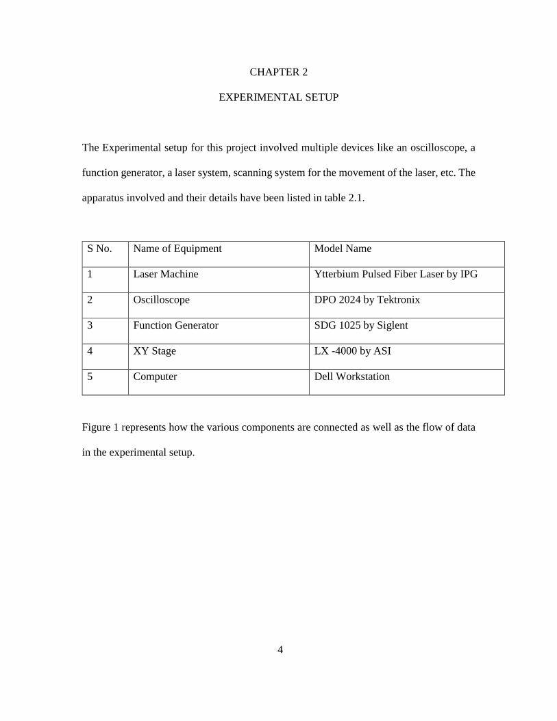
The Experimental setup for this project involved multiple devices like an oscilloscope, a
function generator, a laser system, scanning system for the movement of the laser, etc. The
apparatus involved and their details have been listed in table 2.1.
S No. Name of Equipment Model Name
1 Laser Machine Ytterbium Pulsed Fiber Laser by IPG
2 Oscilloscope DPO 2024 by Tektronix
3 Function Generator SDG 1025 by Siglent
4 XY Stage LX -4000 by ASI
5 Computer Dell Workstation
Figure 1 represents how the various components are connected as well as the flow of data
in the experimental setup.
5
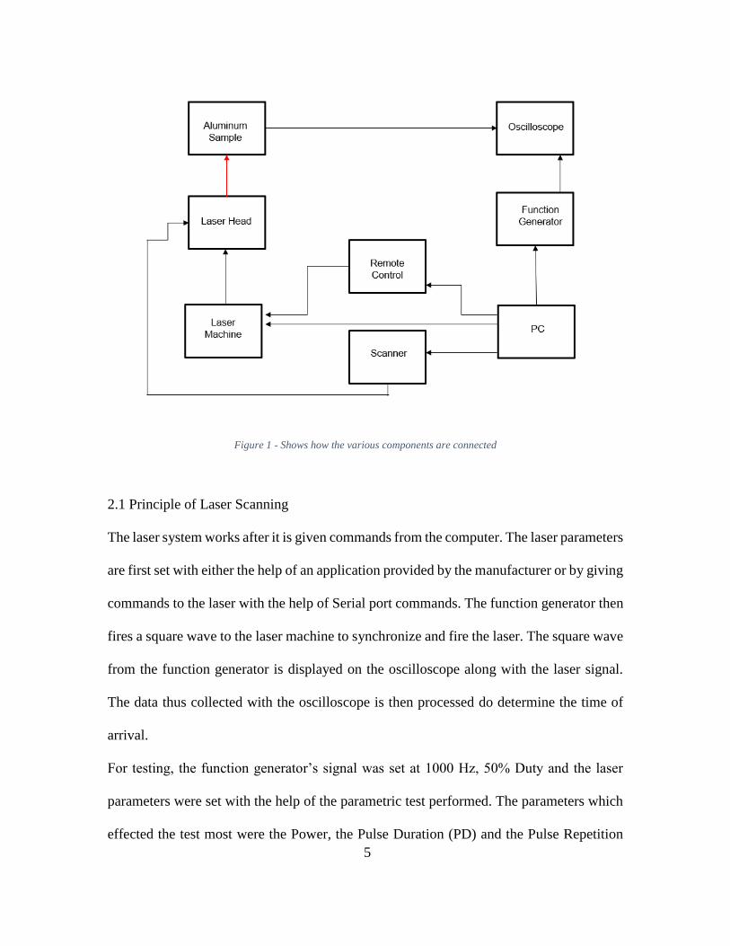
Figure 1 - Shows how the various components are connected
2.1 Principle of Laser Scanning
The laser system works after it is given commands from the computer. The laser parameters
are first set with either the help of an application provided by the manufacturer or by giving
commands to the laser with the help of Serial port commands. The function generator then
fires a square wave to the laser machine to synchronize and fire the laser. The square wave
from the function generator is displayed on the oscilloscope along with the laser signal.
The data thus collected with the oscilloscope is then processed do determine the time of
arrival.
For testing, the function generator’s signal was set at 1000 Hz, 50% Duty and the laser
parameters were set with the help of the parametric test performed. The parameters which
effected the test most were the Power, the Pulse Duration (PD) and the Pulse Repetition
6
Rate (PRR). The parameters were set as 90% Power, 200 ns PD and 60 kHz PRR for test
2.2.2 and 20 kHz for the other tests.
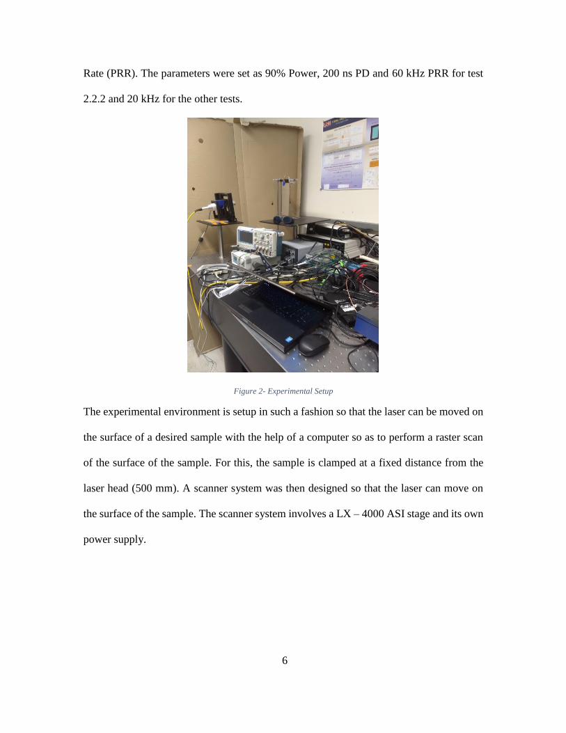
Figure 2- Experimental Setup
The experimental environment is setup in such a fashion so that the laser can be moved on
the surface of a desired sample with the help of a computer so as to perform a raster scan
of the surface of the sample. For this, the sample is clamped at a fixed distance from the
laser head (500 mm). A scanner system was then designed so that the laser can move on
the surface of the sample. The scanner system involves a LX – 4000 ASI stage and its own
power supply.
7
2.2 Tests Conducted
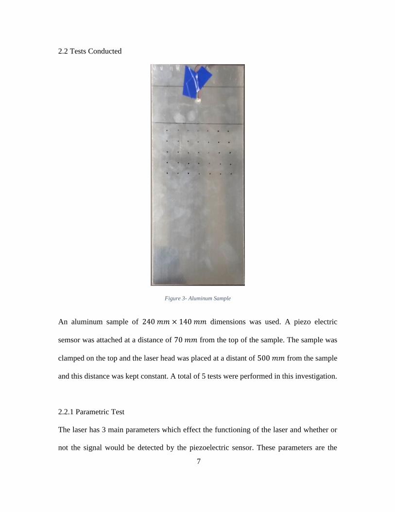
Figure 3- Aluminum Sample
An aluminum sample of 240 𝑚𝑚 × 140 𝑚𝑚 dimensions was used. A piezo electric
semsor was attached at a distance of 70 𝑚𝑚 from the top of the sample. The sample was
clamped on the top and the laser head was placed at a distant of 500 𝑚𝑚 from the sample
and this distance was kept constant. A total of 5 tests were performed in this investigation.
2.2.1 Parametric Test
The laser has 3 main parameters which effect the functioning of the laser and whether or
not the signal would be detected by the piezoelectric sensor. These parameters are the
8
Figure 4 - Path of the laser
power supplied to for the laser generation, the pulse duration of the laser and the pulse
repetition rate of the laser. The power is measured in percentage of the maximum power,
pulse duration (PD) in nanoseconds and the pulse repetition (PRR) rate in kHz. A test was
performed to determine the best combination of these three parameters which was used for
the other three parameters.
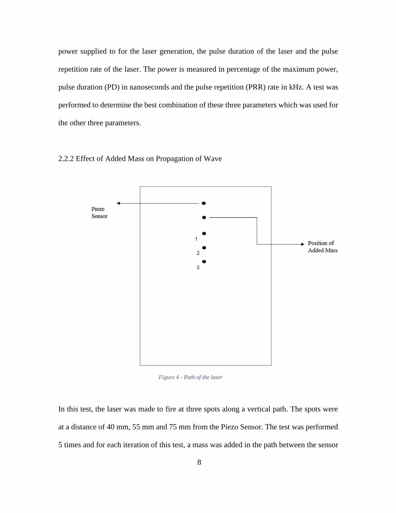
2.2.2 Effect of Added Mass on Propagation of Wave
In this test, the laser was made to fire at three spots along a vertical path. The spots were
at a distance of 40 mm, 55 mm and 75 mm from the Piezo Sensor. The test was performed
5 times and for each iteration of this test, a mass was added in the path between the sensor
9
and the spots where the laser was fired at a distance of 15 mm from the sensor. The laser
parameters for this test were set as 90% Power, 200 ns PD and 60 kHz PRR
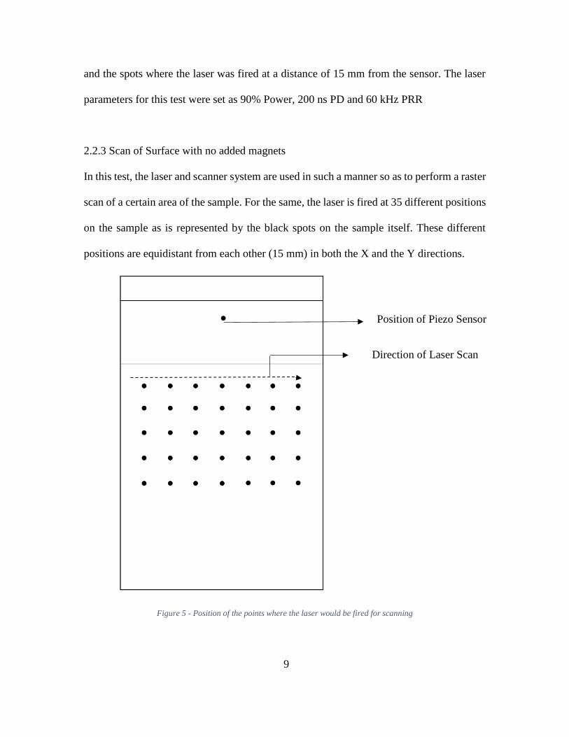
2.2.3 Scan of Surface with no added magnets
In this test, the laser and scanner system are used in such a manner so as to perform a raster
scan of a certain area of the sample. For the same, the laser is fired at 35 different positions
on the sample as is represented by the black spots on the sample itself. These different
positions are equidistant from each other (15 mm) in both the X and the Y directions.
Figure 5 - Position of the points where the laser would be fired for scanning
Position of Piezo Sensor
Direction of Laser Scan
10
A regression analysis using the data from this test was also performed to approximate and
compare the value of the wave speed.
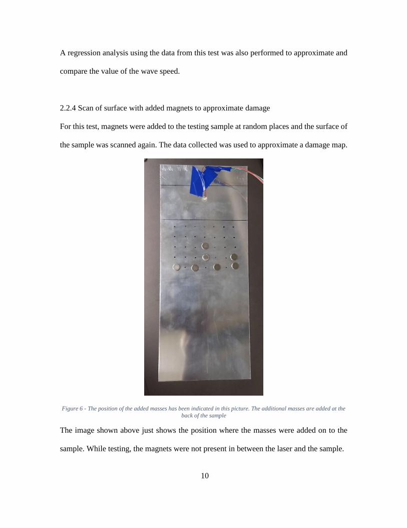
2.2.4 Scan of surface with added magnets to approximate damage
For this test, magnets were added to the testing sample at random places and the surface of
the sample was scanned again. The data collected was used to approximate a damage map.
Figure 6 - The position of the added masses has been indicated in this picture. The additional masses are added at the
back of the sample
The image shown above just shows the position where the masses were added on to the
sample. While testing, the magnets were not present in between the laser and the sample.
11
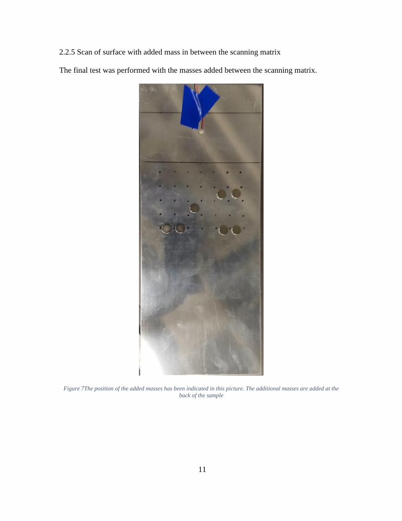
2.2.5 Scan of surface with added mass in between the scanning matrix
The final test was performed with the masses added between the scanning matrix.
Figure 7The position of the added masses has been indicated in this picture. The additional masses are added at the
back of the sample
12
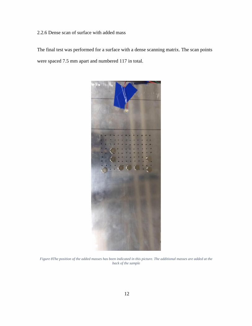
2.2.6 Dense scan of surface with added mass
The final test was performed for a surface with a dense scanning matrix. The scan points
were spaced 7.5 mm apart and numbered 117 in total.
Figure 8The position of the added masses has been indicated in this picture. The additional masses are added at the
back of the sample
13
2.3 Difficulties in Testing
The testing procedure had a few challenges, some of them being of import –
• The selection of proper parameters for the laser testing was challenging and thus
necessitated a parametric study of the laser parameters.
• Inclusion of the scanner system was troublesome as there was no optimal way to
holster the laser head onto the xy stages without damaging either in the process. A
makeshift holster needed to be created to combine both the individual systems
together to form a laser scanning system.
14
CHAPTER 3
DATA PROCESSING AND RESULTS
In this section the procedure behind the processing of the raw data as well as the results
of the aforementioned tests would be discussed. For this project, the time of arrival of the
wave was chosen as the parameter for differentiating between damaged and normal
points as there was no significant change observed in the frequency and the amplitude
changes were difficult to quantify as compared to time of arrival which was easily
determined.
3.1 Data processing
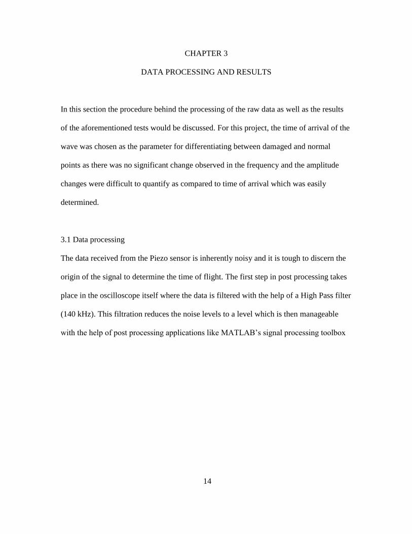
The data received from the Piezo sensor is inherently noisy and it is tough to discern the
origin of the signal to determine the time of flight. The first step in post processing takes
place in the oscilloscope itself where the data is filtered with the help of a High Pass filter
(140 kHz). This filtration reduces the noise levels to a level which is then manageable
with the help of post processing applications like MATLAB’s signal processing toolbox
15
Figure 9 - Data without any Filtering
Figure 10 Data after filtering in the oscilloscope
16
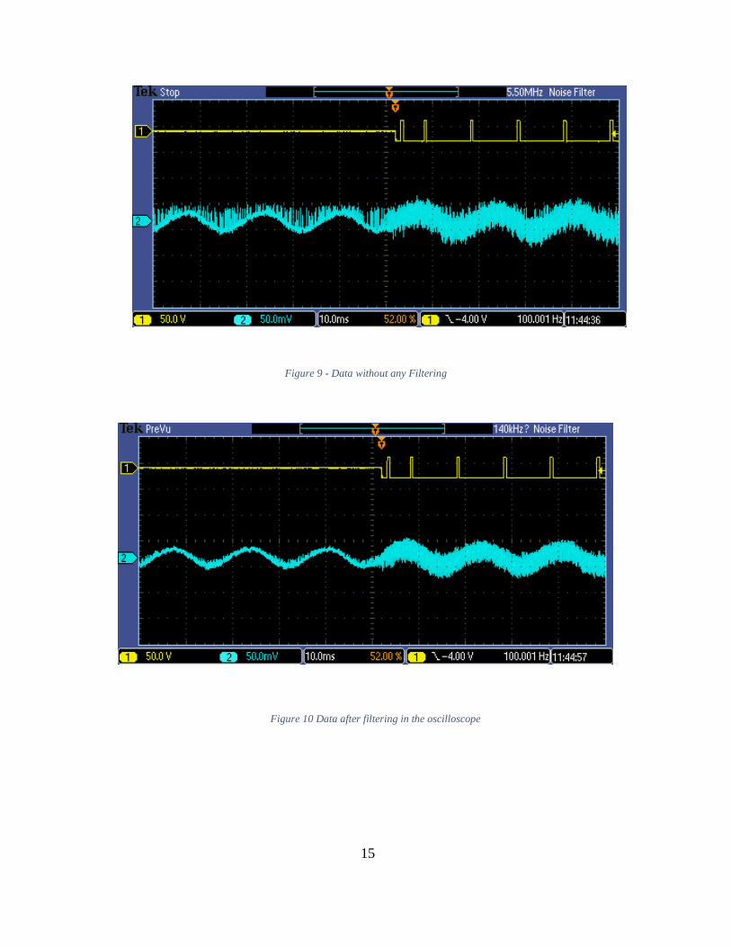
The data after being filtered from oscilloscope is stored in a flash drive and then processed
on a remote computer. It is first filtered with the help of a Butterworth Bandpass filter and
then an empirical mode decomposition is performed along with a Hilbert Spectral analysis
to determine the origin of the signal. This entire process is also called the Hilbert-Huang
transform.
Figure 11 Signal data after Empirical Modal Decomposition
As can be seen, after the post processing we can easily determine the origin of the signal.
This time difference is used to determine the time of arrival of the signal.
17
3.2 Results
The results of all the tests are covered in their own section. After the data was processed it
was tabulated for all the spots as well plotted with respect to the corresponding distance
from the Piezo Sensor
3.2.1 Parametric Test
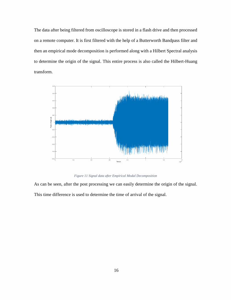
For the parametric study, the laser was fired at a spot which was at a distance of 100 mm
from the laser the variation of the Laser Power had very little effect on the received signal.
As long as the power was above 90%, the signal was clearly received. The laser can only
operate at eight specific Pulse Duration values that is, 4ns, 8ns, 14ns, 20ns, 30ns, 50ns,
100ns, 200ns. These values can be selected both from the laser device application as well
as by sending commands to the laser using the serial port. Four sets of pulse repetition rate
values were chosen for the parametric test; < 20 kHz, 20 kHz to 60 kHz, 60 kHz to 100
kHz and 100 kHz to 140 kHz. The following table shows the parametric study for the
influence of the pulse duration and pulse repetition rate on the laser signal.
Table 1- Results of the parametric Test
18
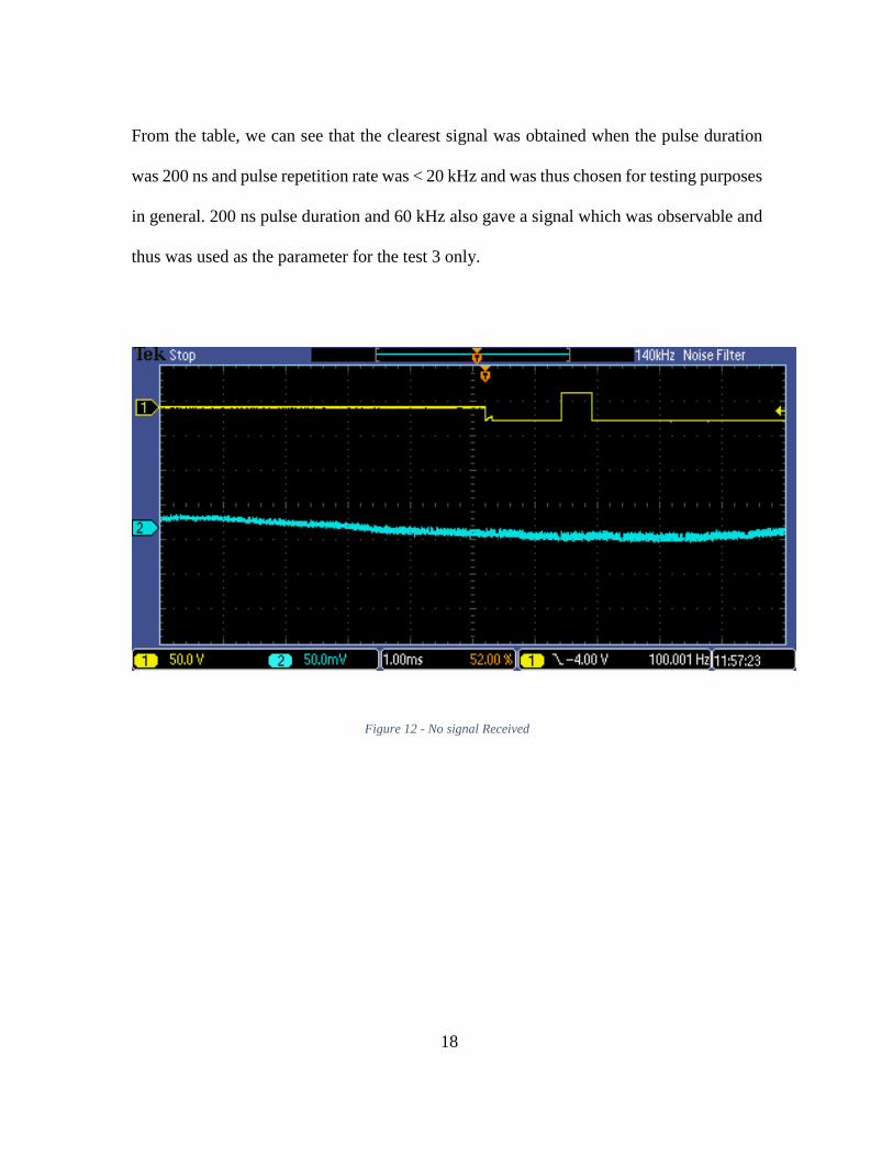
From the table, we can see that the clearest signal was obtained when the pulse duration
was 200 ns and pulse repetition rate was < 20 kHz and was thus chosen for testing purposes
in general. 200 ns pulse duration and 60 kHz also gave a signal which was observable and
thus was used as the parameter for the test 3 only.
Figure 12 - No signal Received
19
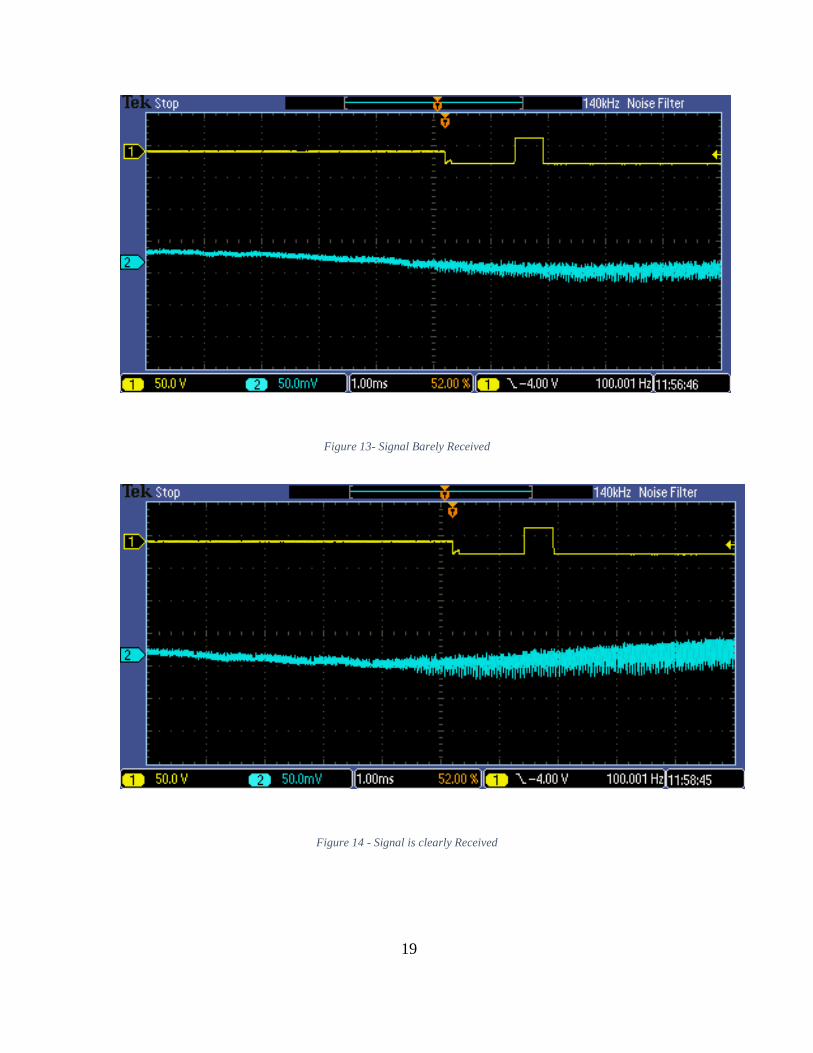
Figure 13- Signal Barely Received
Figure 14 - Signal is clearly Received
20
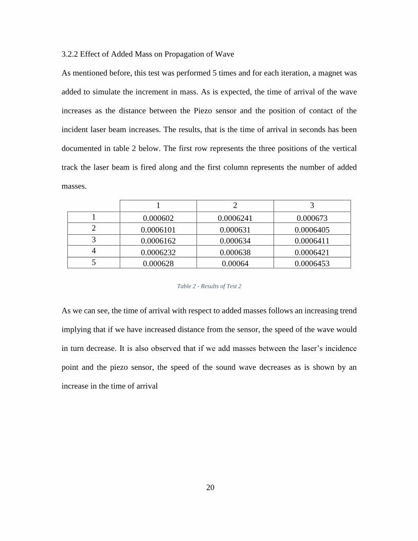
3.2.2 Effect of Added Mass on Propagation of Wave
As mentioned before, this test was performed 5 times and for each iteration, a magnet was
added to simulate the increment in mass. As is expected, the time of arrival of the wave
increases as the distance between the Piezo sensor and the position of contact of the
incident laser beam increases. The results, that is the time of arrival in seconds has been
documented in table 2 below. The first row represents the three positions of the vertical
track the laser beam is fired along and the first column represents the number of added
masses.
1 2 3
1 0.000602 0.0006241 0.000673
2 0.0006101 0.000631 0.0006405
3 0.0006162 0.000634 0.0006411
4 0.0006232 0.000638 0.0006421
5 0.000628 0.00064 0.0006453
Table 2 - Results of Test 2
As we can see, the time of arrival with respect to added masses follows an increasing trend
implying that if we have increased distance from the sensor, the speed of the wave would
in turn decrease. It is also observed that if we add masses between the laser’s incidence
point and the piezo sensor, the speed of the sound wave decreases as is shown by an
increase in the time of arrival
21
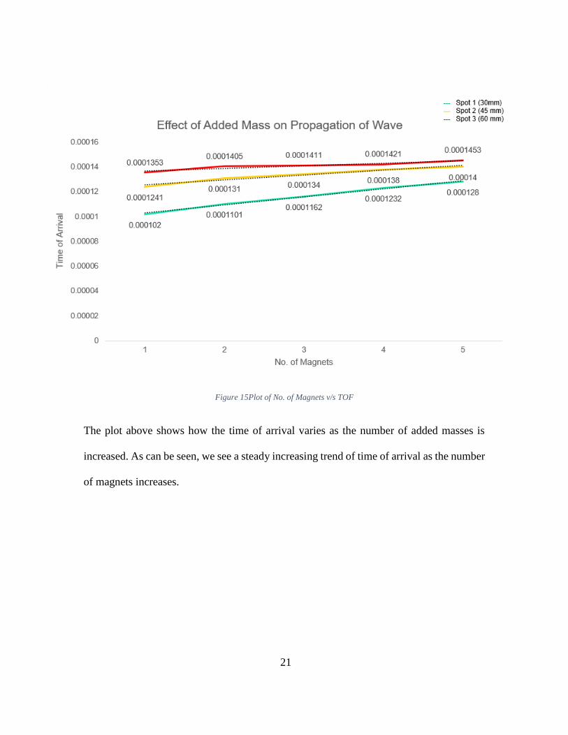
Figure 15Plot of No. of Magnets v/s TOF
The plot above shows how the time of arrival varies as the number of added masses is
increased. As can be seen, we see a steady increasing trend of time of arrival as the number
of magnets increases.
22
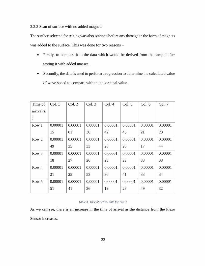
3.2.3 Scan of surface with no added magnets
The surface selected for testing was also scanned before any damage in the form of magnets
was added to the surface. This was done for two reasons –
• Firstly, to compare it to the data which would be derived from the sample after
testing it with added masses.
• Secondly, the data is used to perform a regression to determine the calculated value
of wave speed to compare with the theoretical value.
Time of
arrival(s
)
Col. 1 Col. 2 Col. 3 Col. 4 Col. 5 Col. 6 Col. 7
Row 1 0.00001
15
0.00001
01
0.00001
30
0.00001
42
0.00001
45
0.00001
21
0.00001
28
Row 2 0.00001
49
0.00001
35
0.00001
33
0.00001
28
0.00001
20
0.00001
17
0.00001
44
Row 3 0.00001
18
0.00001
27
0.00001
26
0.00001
23
0.00001
22
0.00001
33
0.00001
38
Row 4 0.00001
21
0.00001
25
0.00001
53
0.00001
36
0.00001
41
0.00001
33
0.00001
34
Row 5 0.00001
51
0.00001
41
0.00001
36
0.00001
19
0.00001
23
0.00001
49
0.00001
32
Table 3- Time of Arrival data for Test 3
As we can see, there is an increase in the time of arrival as the distance from the Piezo
Sensor increases.
23
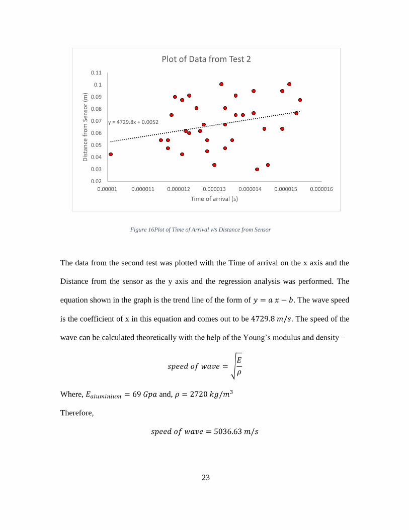
The data from the second test was plotted with the Time of arrival on the x axis and the
Distance from the sensor as the y axis and the regression analysis was performed. The
equation shown in the graph is the trend line of the form of 𝑦 = 𝑎 𝑥 − 𝑏. The wave speed
is the coefficient of x in this equation and comes out to be 4729.8 𝑚/𝑠. The speed of the
wave can be calculated theoretically with the help of the Young’s modulus and density –
𝑠𝑝𝑒𝑒𝑑 𝑜𝑓 𝑤𝑎𝑣𝑒 = √𝐸
𝜌
Where, 𝐸𝑎𝑙𝑢𝑚𝑖𝑛𝑖𝑢𝑚 = 69 𝐺𝑝𝑎 and, 𝜌 = 2720 𝑘𝑔/𝑚3
Therefore,
𝑠𝑝𝑒𝑒𝑑 𝑜𝑓 𝑤𝑎𝑣𝑒 = 5036.63 𝑚/𝑠
y = 4729.8x + 0.0052
0.02
0.03
0.04
0.05
0.06
0.07
0.08
0.09
0.1
0.11
0.00001 0.000011 0.000012 0.000013 0.000014 0.000015 0.000016
Dis
tan
ce f
rom
Sen
sor
(m)
Time of arrival (s)
Plot of Data from Test 2
Figure 16Plot of Time of Arrival v/s Distance from Sensor
24
As we can see, our experimental setup gauges the time of arrival properly as is evidenced
by the closeness of the experimental and theoretical wave speed values.
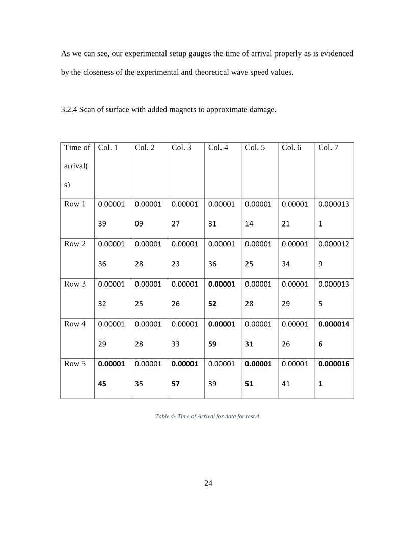
3.2.4 Scan of surface with added magnets to approximate damage.
Time of
arrival(
s)
Col. 1 Col. 2 Col. 3 Col. 4 Col. 5 Col. 6 Col. 7
Row 1 0.00001
39
0.00001
09
0.00001
27
0.00001
31
0.00001
14
0.00001
21
0.000013
1
Row 2 0.00001
36
0.00001
28
0.00001
23
0.00001
36
0.00001
25
0.00001
34
0.000012
9
Row 3 0.00001
32
0.00001
25
0.00001
26
0.00001
52
0.00001
28
0.00001
29
0.000013
5
Row 4 0.00001
29
0.00001
28
0.00001
33
0.00001
59
0.00001
31
0.00001
26
0.000014
6
Row 5 0.00001
45
0.00001
35
0.00001
57
0.00001
39
0.00001
51
0.00001
41
0.000016
1
Table 4- Time of Arrival for data for test 4
25
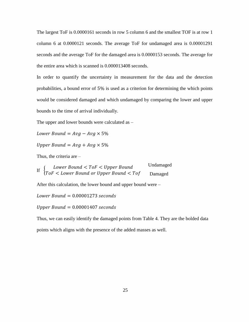
The largest ToF is 0.0000161 seconds in row 5 column 6 and the smallest TOF is at row 1
column 6 at 0.0000121 seconds. The average ToF for undamaged area is 0.00001291
seconds and the average ToF for the damaged area is 0.0000153 seconds. The average for
the entire area which is scanned is 0.000013408 seconds.
In order to quantify the uncertainty in measurement for the data and the detection
probabilities, a bound error of 5% is used as a criterion for determining the which points
would be considered damaged and which undamaged by comparing the lower and upper
bounds to the time of arrival individually.
The upper and lower bounds were calculated as –
𝐿𝑜𝑤𝑒𝑟 𝐵𝑜𝑢𝑛𝑑 = 𝐴𝑣𝑔 − 𝐴𝑣𝑔 × 5%
𝑈𝑝𝑝𝑒𝑟 𝐵𝑜𝑢𝑛𝑑 = 𝐴𝑣𝑔 + 𝐴𝑣𝑔 × 5%
Thus, the criteria are –
If {𝐿𝑜𝑤𝑒𝑟 𝐵𝑜𝑢𝑛𝑑 < 𝑇𝑜𝐹 < 𝑈𝑝𝑝𝑒𝑟 𝐵𝑜𝑢𝑛𝑑
𝑇𝑜𝐹 < 𝐿𝑜𝑤𝑒𝑟 𝐵𝑜𝑢𝑛𝑑 𝑜𝑟 𝑈𝑝𝑝𝑒𝑟 𝐵𝑜𝑢𝑛𝑑 < 𝑇𝑜𝑓
After this calculation, the lower bound and upper bound were –
𝐿𝑜𝑤𝑒𝑟 𝐵𝑜𝑢𝑛𝑑 = 0.00001273 𝑠𝑒𝑐𝑜𝑛𝑑𝑠
𝑈𝑝𝑝𝑒𝑟 𝐵𝑜𝑢𝑛𝑑 = 0.00001407 𝑠𝑒𝑐𝑜𝑛𝑑𝑠
Thus, we can easily identify the damaged points from Table 4. They are the bolded data
points which aligns with the presence of the added masses as well.
Undamaged
Damaged
26
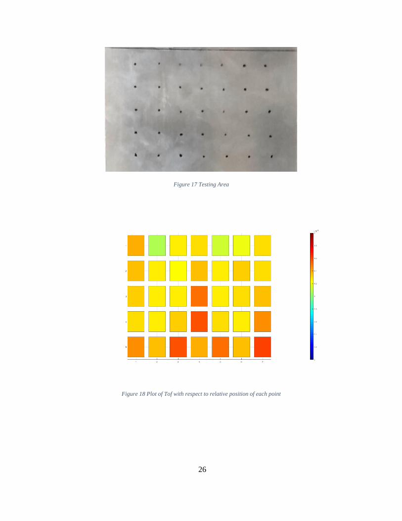
Figure 17 Testing Area
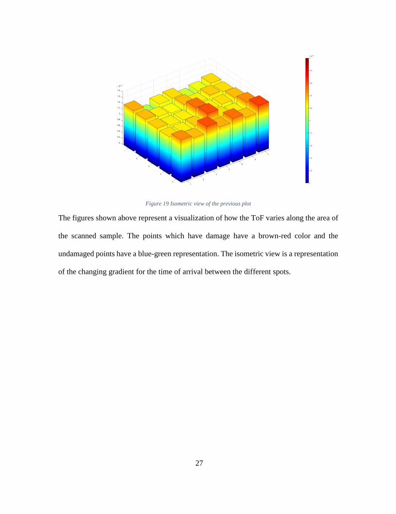
Figure 18 Plot of Tof with respect to relative position of each point
27
Figure 19 Isometric view of the previous plot
The figures shown above represent a visualization of how the ToF varies along the area of
the scanned sample. The points which have damage have a brown-red color and the
undamaged points have a blue-green representation. The isometric view is a representation
of the changing gradient for the time of arrival between the different spots.
28
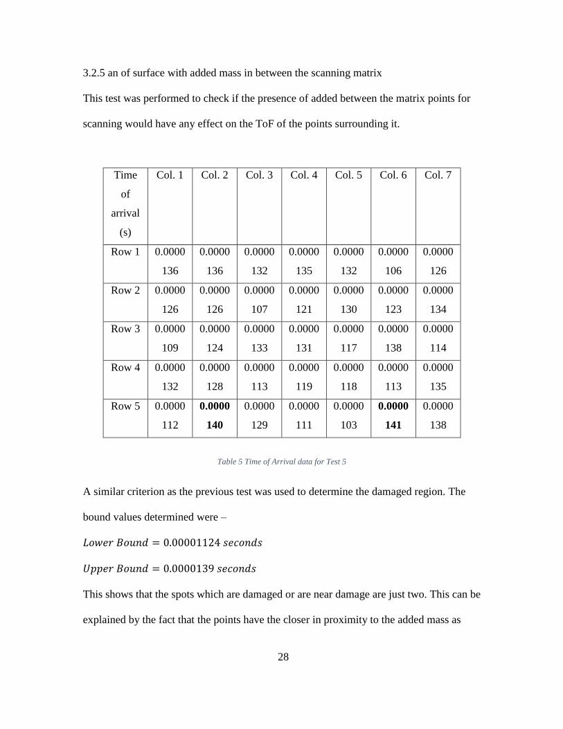
3.2.5 an of surface with added mass in between the scanning matrix
This test was performed to check if the presence of added between the matrix points for
scanning would have any effect on the ToF of the points surrounding it.
Time
of
arrival
(s)
Col. 1 Col. 2 Col. 3 Col. 4 Col. 5 Col. 6 Col. 7
Row 1 0.0000
136
0.0000
136
0.0000
132
0.0000
135
0.0000
132
0.0000
106
0.0000
126
Row 2 0.0000
126
0.0000
126
0.0000
107
0.0000
121
0.0000
130
0.0000
123
0.0000
134
Row 3 0.0000
109
0.0000
124
0.0000
133
0.0000
131
0.0000
117
0.0000
138
0.0000
114
Row 4 0.0000
132
0.0000
128
0.0000
113
0.0000
119
0.0000
118
0.0000
113
0.0000
135
Row 5 0.0000
112
0.0000
140
0.0000
129
0.0000
111
0.0000
103
0.0000
141
0.0000
138
Table 5 Time of Arrival data for Test 5
A similar criterion as the previous test was used to determine the damaged region. The
bound values determined were –
𝐿𝑜𝑤𝑒𝑟 𝐵𝑜𝑢𝑛𝑑 = 0.00001124 𝑠𝑒𝑐𝑜𝑛𝑑𝑠
𝑈𝑝𝑝𝑒𝑟 𝐵𝑜𝑢𝑛𝑑 = 0.0000139 𝑠𝑒𝑐𝑜𝑛𝑑𝑠
This shows that the spots which are damaged or are near damage are just two. This can be
explained by the fact that the points have the closer in proximity to the added mass as
29
compared to the other points and thus the time of arrival for these points is directly
influenced because of their presence.
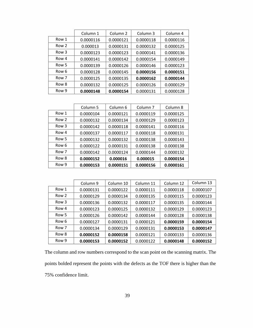
3.2.6 Dense scan of Surface
The data from the dense scan has been tabulated in the Appendix.
The data from this test was significant in number and thus a Gaussian distribution was fit
to the data with the help of MATLAB to develop a criterion for determining the defective
points with the help of their ToF. The distribution thus determined had,
𝜇 = 1.34 × 10⁻⁵ & 𝜎 = 1.28 × 10⁻⁶
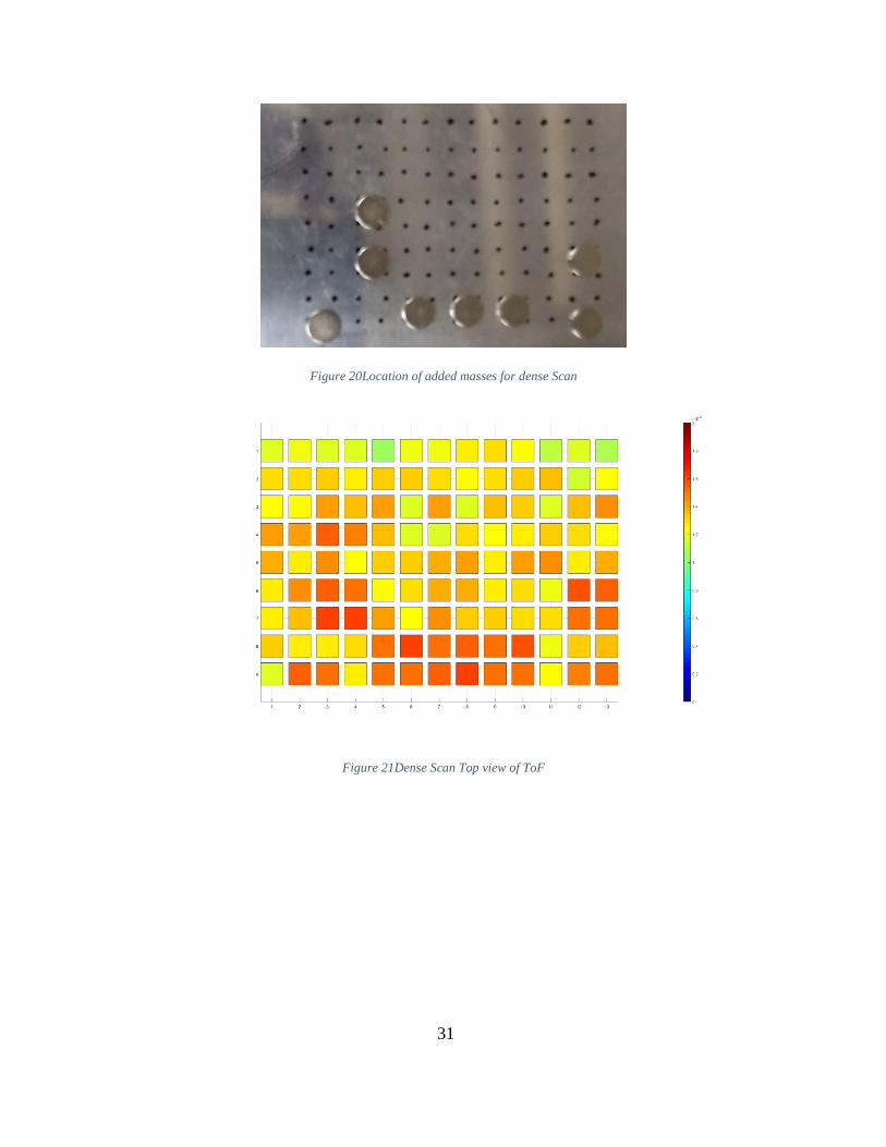
Since the test involves masses being added to simulate damage, implying that the density
at that point would be higher, the ToF for a defective point thus would be higher than the
general ToF. Thus, the criteria was that if the values lie in the cumulative probabilities for
positive z-values for a certain confidence level, they would be non-defective. The
confidence levels chosen were 95%, 90%, 85%, 80% and 75%.
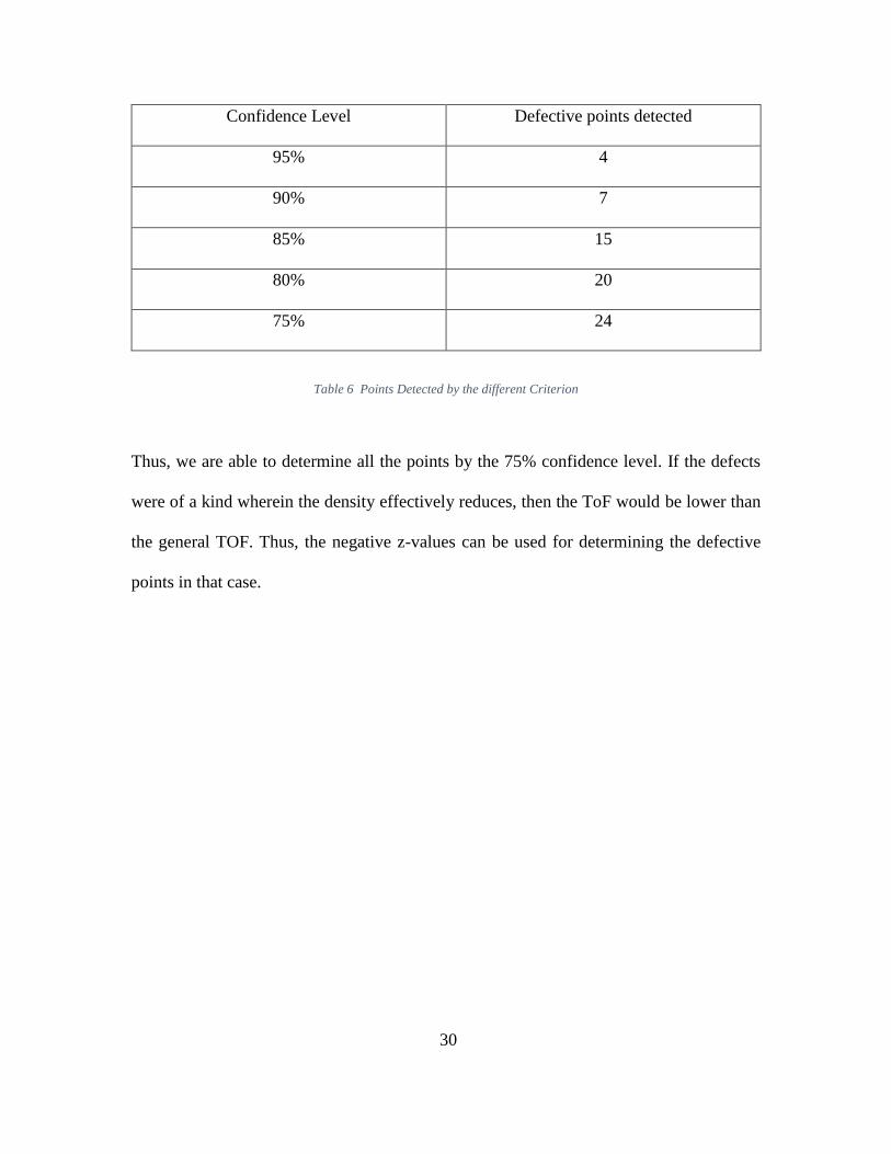
According to the scanned region, a total of 24 points should have been identified as
defective. The different confidence levels were able to determine the points with defective
ToF with varying success.
30
Confidence Level Defective points detected
95% 4
90% 7
85% 15
80% 20
75% 24
Table 6 Points Detected by the different Criterion
Thus, we are able to determine all the points by the 75% confidence level. If the defects
were of a kind wherein the density effectively reduces, then the ToF would be lower than
the general TOF. Thus, the negative z-values can be used for determining the defective
points in that case.
31
Figure 20Location of added masses for dense Scan
Figure 21Dense Scan Top view of ToF
32
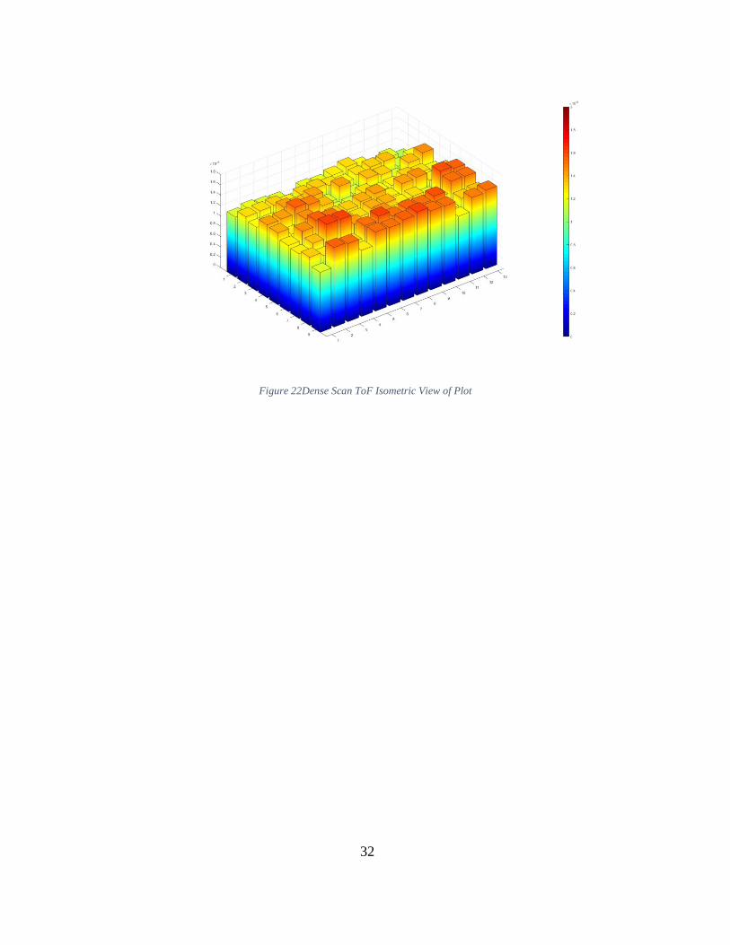
Figure 22Dense Scan ToF Isometric View of Plot
33
CHAPTER 4
CONCLUSION AND FUTURE WORK
Laser scanning technology is a widely used method for damage detection and has
extremely varied applications. It is a valuable technique as it is a non-destructive technique
which is not only cheap but in most cases is easy to setup and use.
This research focused on developing a novel method for using laser induced ultrasonic
waves for non-destructive testing. To that end first a scanning system needed to be
developed so that the laser could moved on the surface of a test sample. This was achieved
by holstering the laser head onto an ASI xy stage which was then controlled by a computer.
Once the scanner system was developed, a series of tests were performed on the sample.
The first was a parametric test which was used to decide the operational parameters of the
laser. The next test was done to determine the effect of added mass on the laser induced
ultrasound and it was found that as the number of added masses increased, so did the time
of arrival.
To establish that the time of arrival determined by this laser scanning method was indeed
logical and the wave speed thus determined would resemble the theoretical values which
can be calculated, the third test involved scanning the surface of the sample to determine
an approximate of the wave speed. This data was then plotted with respect to the distance
from the piezoelectric sensor and a linear regression was performed to determine the speed
of the ultrasound wave. The speed of the wave determined in such a fashion was found to
be close to the value which can be calculated theoretically.
34
The fourth test was a scan of the surface after masses were added to the sample’s surface
to visualize damage. The data from this test was plotted and a criterion was determined to
estimate the points which had damage. The damaged points determined from this criterion
was a perfect match to the damaged points actually present. Thus, this method was found
to be able to determine whether or not a point is damaged if the laser is fired on that specific
point. The fifth test’s purpose was to determine if the time of arrival would be affected if
the added mass in between the scanning matrix. A similar criterion as test four was used in
this test as well to find the damaged points. The criteria however only found two points to
be damaged leading to the conclusion that unless the damaged region is in close proximity
or in the path of the incidence of the laser beam, the time of arrival would not be affected.
For the final test, the scanning matrix was made denser so as to increase the number of
scanning points and masses were added to simulate damage. As the number of points
scanned in this test was more, a Normal distribution was fit to this data with the help of
MATLAB. As mass is only added to the surface, it was assumed that any ToF which is
significantly higher would be defective. Thus, the data in the positive confidence limit was
assumed to be non-defective and higher than that was defective. It was found that 80%
confidence was able to detect the most defective points easily.
In future, the entire scanning system can be improved so that more minute movements of
the laser is possible so as to improve the resolution of the scan. The scanning system also
needs to be made more robust so that the scanning of a larger area of the sample is possible.

35
The regression study performed in test 3 for the wave speed was only performed for 35
points. The sample size an be increased for a more accurate value of the wave speed. In
this study, the test number 4 was only performed with a single added mass on each of the
damaged points. For future testing the effect of the increase in the number of added masses
on the time of arrival is something which needs to be studied.
36
REFERENCES
1. Ihn, J., & Chang, F. (2004). Detection and monitoring of hidden fatigue crack
growth using a built-in piezoelectric sensor/actuator network: II. Validation using
riveted joints and repair patches. Smart Materials and Structures, 13(3), 621-630.
doi:10.1088/0964-1726/13/3/021
2. Harb, M., & Yuan, F. (2015). A rapid, fully non-contact, hybrid system for
generating Lamb wave dispersion curves. Ultrasonics, 61, 62-70.
doi:10.1016/j.ultras.2015.03.006
3. Huang, N. E. (n.d.). An Adaptive Data Analysis Method for Nonlinear and
Nonstationary Time Series: The Empirical Mode Decomposition and Hilbert
Spectral Analysis. Wavelet Analysis and Applications Applied and Numerical
Harmonic Analysis, 363-376. doi:10.1007/978-3-7643-7778-6_25
4. K. Dragan, M. Dziendzikowski, T. Uhl, and L. Ambrozinski, “Damage detection
in the aircraft structure with the use of integrated sensors - SYMOST project,” Proc.
6th Eur. Work. - Struct. Heal. Monit. 2012, EWSHM 2012, vol. 2, pp. 974–980,
2012
5. W. Ostachowicz, T. Wandowski, and P. Malinowski, “Damage Detection Using
Laser Vibrometry,” NDT Aerosp., pp. 1–8, 2010.
6. M. Ochiai, “Development and Applications of Laser-ultrasonic Testing in Nuclear
Industry,” Int. Symp. Laser Ultrason. Sci. Technol. Appl., vol. Science, T, no.
March, pp. 4–12, 2008.
7. L. Mallet, B. C. Lee, W. J. Staszewski, and F. Scarpa, “Structural health monitoring
using scanning laser vibrometry: II. Lamb waves for damage detection,” Smart
Mater. Struct., vol. 13, no. 2, pp. 261–269, 2004.
8. S. E. Burrows, S. Dixon, S. G. Pickering, T. Li, and D. P. Almond, “Thermographic
detection of surface breaking defects using a scanning laser source,” NDT E Int.,
vol. 44, no. 7, pp. 589–596, 2011.
9. Yantchev, V., & Katardjiev, I. (2013). Thin film Lamb wave resonators in
frequency control and sensing applications: A review. Journal of Micromechanics
and Microengineering, 23(4), 043001. doi:10.1088/0960-1317/23/4/043001

37
10. Kessler, S. S., Spearing, S. M., & Soutis, C. (2002). Damage detection in
composite materials using Lamb wave methods. Smart Materials and Structures,
11(2), 269-278. doi:10.1088/0964-1726/11/2/310

38
APPENDIX A
TOF DATA FOR TEST 6
39
Column 1 Column 2 Column 3 Column 4
Row 1 0.0000116 0.0000121 0.0000118 0.0000116
Row 2 0.000013 0.0000131 0.0000132 0.0000125
Row 3 0.0000123 0.0000123 0.0000141 0.0000136
Row 4 0.0000141 0.0000142 0.0000154 0.0000149
Row 5 0.0000139 0.0000126 0.0000146 0.0000123
Row 6 0.0000128 0.0000145 0.0000156 0.0000151
Row 7 0.0000125 0.0000135 0.0000162 0.0000144
Row 8 0.0000132 0.0000125 0.0000126 0.0000129
Row 9 0.0000148 0.0000154 0.0000131 0.0000128
Column 5 Column 6 Column 7 Column 8
Row 1 0.0000104 0.0000121 0.0000119 0.0000125
Row 2 0.0000132 0.0000134 0.0000129 0.0000123
Row 3 0.0000142 0.0000118 0.0000141 0.0000116
Row 4 0.0000137 0.0000117 0.0000118 0.0000131
Row 5 0.0000132 0.0000132 0.0000138 0.0000143
Row 6 0.0000122 0.0000131 0.0000138 0.0000138
Row 7 0.0000142 0.0000124 0.0000144 0.0000132
Row 8 0.0000152 0.000016 0.000015 0.0000154
Row 9 0.0000153 0.0000151 0.0000156 0.0000161
Column 9 Column 10 Column 11 Column 12 Column 13
Row 1 0.0000131 0.0000122 0.0000111 0.0000118 0.0000107
Row 2 0.0000129 0.0000134 0.0000135 0.0000115 0.0000123
Row 3 0.0000136 0.0000132 0.0000117 0.0000135 0.0000144
Row 4 0.0000123 0.0000125 0.0000132 0.0000129 0.0000123
Row 5 0.0000126 0.0000142 0.0000144 0.0000128 0.0000138
Row 6 0.0000127 0.0000131 0.0000121 0.0000159 0.0000154
Row 7 0.0000134 0.0000129 0.0000131 0.0000153 0.0000147
Row 8 0.0000152 0.0000158 0.0000121 0.0000133 0.0000136
Row 9 0.0000153 0.0000152 0.0000122 0.0000148 0.0000152
The column and row numbers correspond to the scan point on the scanning matrix. The
points bolded represent the points with the defects as the TOF there is higher than the
75% confidence limit.

40
APPENDIX B
MATLAB COMMANDS UTILIZED

41
Three major MATLAB commands were used in this project.
• The first is 𝑒𝑚𝑑 which is used to perform the empirical modal decomposition
of the signal data to determine the ToF.
• The second major command was the 𝑓𝑖𝑡𝑑𝑖𝑠𝑡 command to fit the Gaussian
distribution to the data from test 6.
• The last major command is the 𝑏𝑎𝑟3 command used for the 3d plots.