EXPERIMENTAL INVESTIGATION OF COOLANT MIXING IN VVER REACTOR FUEL BUNDLES BY PARTICLE IMAGE VELOCIMETRY

D. Tar, G. Baranyai, Gy. Ézsol, I. Tóth

Hungarian Academy of Sciences KFKI Atomic Energy Research Institute Budapest P.O. Box 49., 1525 Hungary; e-mail: tar@aeki.kfki.hu

Abstract The coolant mixing in the head part of a fuel assembly of a VVER reactor has been experimentally investigated by particle image velocimetry (PIV). By measuring the whole flow field velocity and temperature distribution the relation between the value produced by the point-based thermocouple measuring the outlet temperature of the coolant and the subchannel outlet temperatures can be established. After performance verification of the system by simple tests, the main experiments have been carried out on a 1:1 size (vertically only 1m long) model of the VVER-440/213 fuel assembly. The two-dimensional PIV velocity vector field results around the core exit thermocouple are highlighted in the paper. The measurements of the turbulent flow of coolant in the regular tube channel around the thermocouple proved that there is rotation and asymmetry in the coolant flow caused by the mixing grid, and the geometrical asymmetry of the fuel bundle. The fuel assembly model will also be used for whole flow field temperature distribution measurements by laser induced fluorescence (LIF), and the final aim is to validate CFD analysis for the head part of the fuel bundle.

1. INTRODUCTION The calculated core exit temperature in Paks NPP is determined conservatively, without taking into account any mixing. The measured values by the thermocouples mounted in the fuel bundle heads – which supply important information for the limitation of the reactor core power – and the average outlet temperatures of the coolant may differ as a consequence of incomplete mixing. Several CFD calculations have been preformed (e.g. Tóth and Aszódi, 2007) and also experimental equipment has been built (Kobzar and Oleksyuk, 2006) to investigate the mixing in the fuel assembly head and for validation of the CFD calculations by the comparison of measurement data. In our laboratory a full scale (vertically 1m long) model of the VVER-440/213 fuel assembly was constructed for the investigation of mixing of subchannel flows with different temperatures and for supplying data for CFD validation. Laser optical measurements were chosen to obtain velocity and temperature distribution by particle image velocimetry (PIV) and laser induced fluorescence (LIF). It is an advantage of PIV and LIF that whole flow field velocity and temperature distributions can be obtained in a non-intrusive manner in contrast with conventional techniques applied for similar experiments cited above. In the course of preliminary laser optical measurements – detailed description can be found in an earlier paper (Tar et al., 2006) – simple models representing a part of the fuel bundle were examined. In this paper the first part of the research project investigating the coolant mixing in the fuel bundle head is reported, which covers velocity distribution results obtained by PIV. The aim of the measurements is to establish an experimental database, as well as the validation of CFD calculations. However, this paper only discusses PIV velocity field results . The laser optical experiments are being continued by whole flow field temperature measurements with the use of the laser induced fluorescence (LIF) technique.

2

2. METHODS 2.1. The fuel bundle model

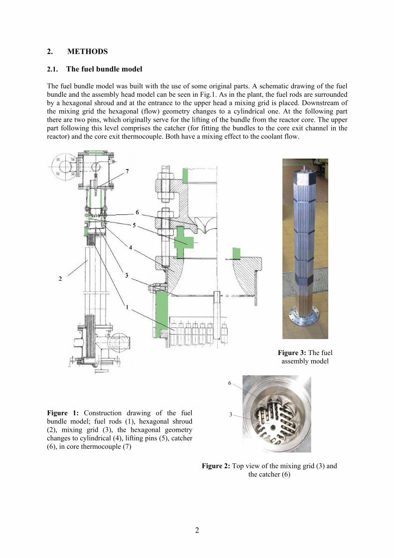
The fuel bundle model was built with the use of some original parts. A schematic drawing of the fuel bundle and the assembly head model can be seen in Fig.1. As in the plant, the fuel rods are surrounded by a hexagonal shroud and at the entrance to the upper head a mixing grid is placed. Downstream of the mixing grid the hexagonal (flow) geometry changes to a cylindrical one. At the following part there are two pins, which originally serve for the lifting of the bundle from the reactor core. The upper part following this level comprises the catcher (for fitting the bundles to the core exit channel in the reactor) and the core exit thermocouple. Both have a mixing effect to the coolant flow.

Figure 3: The fuel assembly model

Figure 1: Construction drawing of the fuel bundle model; fuel rods (1), hexagonal shroud (2), mixing grid (3), the hexagonal geometry changes to cylindrical (4), lifting pins (5), catcher (6), in core thermocouple (7)

Figure 2: Top view of the mixing grid (3) and

the catcher (6)

3

In Figs. 2 and 3 the top view of the mixing grid with the catcher and the fuel assembly model can be seen, respectively. The following parts of the model were made of glass and PMMA (plexiglas) in order to be transparent for the laser beam (green zones in Fig.1): − The 200 mm long tube part, comprising the outlet thermocouple. The coolant stream conditions

(velocity and temperature distributions) around the thermocouple housing can be investigated here.

− The tube part before the catcher is 40 mm long, it comprises the two lifting pins, which also have an influence on the velocity distributions.

− At the hexagonal part of the fuel bundle three measuring windows were created with a 120° symmetry, where the velocity and temperature distribution of the coolant leaving the fuel rods can be measured.

− The window on the top of the model enables recording the flow distribution in the cross section area, i.e. measuring the velocities in the horizontal plane.

In Figs. 4 and 5 a photo of the hydraulic loop, and that of the test section along with the PIV system are shown. 2.2. Overview of the PIV system and the measuring parameters Characteristics of the system are described in detail in an earlier paper (Tar, 2006), here only the main PIV parameters are summarised as they were typically adjusted for the measurements. The energy of the Nd YAG laser was set to 20% of the maximum 50 mJ, the diameter of the polyamide seeding particles were 20 µm, the typical interrogation area size was 16×16 pixel, and cross correlation was used for the calculation (Dantec, 2000). The time between the two laser impulses (∆t, resulting in two particle images) was set to 100 µs. The time averaged velocity field results reported in the following sub-sections have been obtained by recording 500 frame pairs at 2 Hz frequency.

Figure 4: The hydraulic loop and the fuel bundle model

Figure 5: The test section and the PIV system

4

3. RESULTS 3.1. Results of the measurements The main question to be answered by the measurement is, whether the flow is perfectly mixed or not around the core exit thermocouple. The measurements were carried out at four axial levels, where the transparent windows are placed (Fig. 1). Figure 6 shows the measurement setup and the time averaged velocity field between the top of the fuel rods and the mixing grid. The scaling factor for the absolute velocity values was calibrated to the central tube of 10.3 mm diameter. In this case the laser beam and the axis of the camera were not at 90°, but at an angle of 120°, as a result, the image recorded are distorted due to the perspective. Images were dewarped with an imaging model fit (camera calibration) describing the distortion (Dantec, 2000). At a flow rate of 90 m3/h the average lengths of the velocity vectors in this flow field were between 0.5 and 2.5 m/s. This proved to be the lowest local velocity in the flow of the whole model. Higher velocity plumes can be observed at the lower part of the image, at the fuel subchannel outlets. Regarding the upper part of the image, the effect of the mixing grid to the flow field can be clearly discovered, as the measured area extended to the mixing grid.

Figure 6: Measuring setup and time averaged velocity field between the top of the fuel rods and the

mixing grid In Fig. 7 the measuring setup and the time averaged velocity field in the area below the catcher can be seen. In this part there are two pins, which in the real fuel bundle serve for the lifting of the assemblies – in the model they were made of PMMA as the cylindrical tube part. For the absolute velocity calibration a ruler was placed to the measurement plane. The lengths of the velocity vectors in this field at 90 m3/h flow rate were between 2 and 4.5 m/s, but in the vicinity of the catcher some higher velocity plumes were observed, exceeding 5 m/s. This proved to be the highest velocity regarding the flow filed of the whole model. The influence of the mixing grid to the flow field can be also clearly discovered around the tube centreline. Around the central part of the mixing grid there is no path for the flow; it changes the upstream flow distribution, causing a low velocity region in the middle of the channel.

I i 65 5 41 6 ( 35 1 22 4) i i l 1772 1126 8 bit

5

0 5 10 15 20 25 30 35 40 45 50 55 60 65 70 75 80 85 90 95 100 105 110 115mm0

5

10

15

20

25

30

35

40

45

50

55

60

65

70

75

80

85mm

Image size: 1600×1186 (0,0), 8-bitsBurst#; rec#: 1; 1 (1), Date: 2008.04.08, Time: 12:36:53:688

Figure 7: Measuring setup and time averaged velocity field below the catcher

For the measurements of the cylindrical tube part (core exit channel, Fig. 8) the scaling factor for the absolute velocities was calibrated to the 8.5 mm diameter tube part of the thermocouple, which appears on the particle image recordings. The vertical components of the maximum velocities are around 4 m/s at 90 m3/h flow rate. The local influence of the thermometer on the time averaged velocity field can be clearly discovered (Fig. 8.a). On the time averaged vector map of the lower part of the tube (Fig.8.b) a low velocity region can be observed at the sides, which is getting narrower in the upper region; this is the influence of the catcher. An instantaneous velocity vector map measured at the lower region is also shown (Fig.8.c). The instantaneous distribution displays the fluctuations of the turbulent flow – on the vector map vortexes and plumes can be seen which disappear in the time averaged case. The chaotic instantaneous distribution is the consequence of the flow mixing effect of the mixing grid and the catcher. The vertical velocity distribution and the time averaged stress terms measured in horizontal profiles of the cylindrical tube part at the elevation of 36 mm on the vector map of Fig. 8.b can be seen in Fig. 9. On the time averaged stress diagrams u means the vertical, v means the horizontal velocity components. Both the velocity and the stress distributions show the typical form for turbulent tube flows. Some asymmetry can be observed, which can be explained by the swirling flow caused by the mixing grid.. This aspect will be investigated in more detail during the course of following measurements, when velocity and temperature distributions will be measured in the horizontal plane through the measuring window on the top of the model (Fig.1).

6

0 5 10 15 20 25 30 35 40 45 50 55 60 65 70mm0

5

10

15

20

25

30

35

40

45

50mm

Statistics vector map: Vector Statistics, 100×74 vectors (7400)Size: 1600×1184 (0,0)

(a)

0 5 10 15 20 25 30 35 40 45 50 55 60 65 70mm0

5

10

15

20

25

30

35

40

45

50mm

Vector map: Filtered, 100×74 vectors (7400), 274 disabled, 7400 substitutedBurst#; rec#: 1; 1 (1), Date: 2008.04.04, Time: 12:57:12:782A l i 2 021 2 039 2 027 2 050

(b)

0 5 10 15 20 25 30 35 40 45 50 55 60 65 70mm0

5

10

15

20

25

30

35

40

45

50mm

Vector map: Filtered, 100×74 vectors (7400), 7400 substitutedBurst#; rec#: 35; 1 (35), Date: 2008.04.03, Time: 12:40:51:859Analog inputs: -2.192; -2.212; -2.197; -2.227

(c)

Figure 8: Measuring setup and time-averaged velocity vector map around the lower part of the

thermometer (a), and at the lower part of the cylindrical tube part (b), and instantaneous velocity vector map (c), v[m/s], Q=90 m3/h

7

Figure 9: Vertical velocity magnitudes, standard deviations, and time averaged stress terms measured

in horizontal profiles of the cylindrical tube part. (Measured at 36 mm level on vector map showed on Fig. 8.b; u means the vertical, v means the horizontal velocity components.)

3.2. Discussion of the accuracy and the uncertainties A detailed general description of the image evaluation methods for PIV and of post-processing of PIV data can be found for example in the work of Raffel (1996). Below the data processing and post processing are looked over only in the case of our installed PIV system. Three main steps have been applied for the post processing of our measured PIV data: validation, time averaging, and space averaging. PIV is an instantaneous measurement technique; all spatial information is sampled at the same time so there will be some regions where there is really no meaningful input and incorrect vectors can occur (Dantec, 2000). In the case of our reported results peak height and velocity range validation have been carried out. Peak height validation validates or rejects individual vectors based on the values of the peak heights in the correlation plane where the vector displacement has been measured. Velocity-range validation rejects vectors, which are outside a certain range (Dantec, 2000). The next step of the post processing has been the time averaging of the set of our acquired data. The time averaging has been realized by calculating mean velocity vector maps. The standard deviations for each velocity components have been also calculated; they are shown on Fig.9 as the uncertainties of the velocity profiles. According the diagrams the magnitude of the vertical velocity fluctuations are lower around the centreline of the tube and higher at the sides at all the three flow rates. The final step of post processing is the filtering vector maps by arithmetic averaging over vector neighbours. Inside the averaging area the individual vectors are smoothed out by the average vector. In earlier papers (Tar, 2006) basic measurements were reported for the assessment of the accuracy and limits of producing velocity vector maps by measuring with the installed PIV system. In the course of the simple, commencing measurements by comparing the results with integrated measured values it was found, that the relative uncertainty of the space and time filtered data of the velocity vector fields was about 5 %. This uncertainty includes the systematic error which source is the determination of the absolute velocities by measuring the scaling factors. The vibration of the hydraulic loop cannot be avoided due to the relatively high flow velocities. The vibration is detectable on the particle images. By choosing correctly the interrogation areas, the effect of the vibration can be corrected on the time averaged vector maps. In the case of the measurements the ∆t (time between the two laser impulses, resulting in two particle images) was set to 100 µs, and the frequency of recording image pairs (vector maps) was 250 ms. It is possible to check a set of image pairs, and mark a fix point of the tube (for example its side) on the image, and notice whether the displacement of the fix point caused by the vibration is smaller or bigger than the size of the interrogation area. By choosing the interrogation area size big enough, the displacement will not

8

exceed its size. The result vector produced by one particle image pair can be interpreted as a spatial average within one interrogation area. By calculating the time averaged vector maps the vectors belonging to the same interrogation area position are averaged in time. The relative uncertainty of the induction flow meter installed in the main line of the loop with the range of 6.4-160 m3/h was < 1.5 % within the applied 50-90 m3/h range. Out of this ± 0.5 % can be assigned to the conversion of the flow velocity to electric signal. 4. CONCLUSION The whole flow field velocity vector map results obtained by PIV measurements compose the first part of the experimental database of the laser optical measurements carried out to investigate the coolant flow mixing in the head part of a fuel assembly model. The velocity fields were measured at three horizontal levels of the bundle; at the regions of the transparent windows according to Fig. 1. At the region where the coolant has just left the fuel rods, higher velocity plumes can be observed; indicating the influence of the subchannels (Fig. 6). The first element in the channel which causes relevant mixing of the flow is the mixing grid. Around the central part of the mixing grid there is no path for the flow; it changes the upstream flow distribution, causing a low velocity region in the middle of the channel. This low velocity region can also be detected downstream of the mixing grid (Fig. 7).. At this elevation the influence of the lifting pins and the catcher determines the flow distribution. The catcher produces higher velocity stream lines; this element is also an important mixing tool like the mixing grid. The catcher also narrows down the stream channel slightly; its effect can be seen on the velocity vector map at the cylindrical tube part (core exit channel, Fig 8.b) as lower velocity regions at the channel wall. Further downstream, near the thermocouple housing the thickness of the lower velocity region is decreasing as a turbulent velocity profile develops (Fig. 8.a). The thermocouple is in the middle of the channel in the highest velocity region. By this elevation the mixing grid, the catcher and the lifting pins have assured sufficient homogenisation of the coolant flow regarding velocity distribution; consequently there is no detectable trace of the high velocity plumes observed at the subchannel outlets. These velocity distribution measurements by PIV will be completed by temperature distribution results measured by LIF, which will allow complex analysis of the coolant mixing. 5. REFERENCES Dantec Measurement Technology, FlowMap® Particle Image Velocimetry Instrumentation (2000)

L.L. Kobzar, D.A. Oleksyuk, Experiments on Simulation of Coolant Mixing in Fuel Assembly Head

and Core Exit Channel of VVER-440 Reactor, 16th Symposium of AER, Slovakia (2006)

M. Raffel, C. Willert, J. Kompenhans, Particle Image Velocimetry, Springer (1996)

D. Tar, G. Baranyai, Gy. Ézsöl, I. Tóth, PIV System for Fluid Flow Measurement in Fuel Assembly of

Nuclear Reactor, Conference on Modelling Fluid Flow, Budapest (2006)

D. Tar, G. Baranyai, Gy. Ézsöl., I. Tóth, Application of PIV for the Measurement of Coolant Flow in

Fuel Assembly, V. Nukleáris Technikai Szimpózium, Paks (2006) – in Hungarian

S. Tóth, A. Aszódi, Preliminary Validation of VVER-440 Fuel Assembly Head CFD Model, 17th

Symposium of AER, Ukraine (2006)