Experimental Analysis of Hybrid Genetic Algorithm for the

335Information Technology and Control 2019/2/48

Experimental Analysis of Hybrid Genetic Algorithm for the Grey Pattern Quadratic Assignment Problem

ITC 2/48Journal of Information Technology and ControlVol. 48 / No. 2 / 2019pp. 335-356DOI 10.5755/j01.itc.48.2.23114

Experimental Analysis of Hybrid Genetic Algorithm for the Grey Pattern Quadratic Assignment Problem

Received 2019/04/08 Accepted after revision 2019/05/09

http://dx.doi.org/10.5755/j01.itc.48.2.23114

Corresponding author: [email protected]

Evelina StanevičienėKaunas University of Technology, Department of Multimedia Engineering, Studentų str. 50-408, LT-51368 Kaunas, Lithuania, tel. +370-37-300373, e-mail: [email protected]

Alfonsas MisevičiusKaunas University of Technology, Department of Multimedia Engineering, Studentų str. 50-416a/400, LT-51368 Kaunas, Lithuania tel. +370-37-300372, e-mail: [email protected]

Armantas OstreikaKaunas University of Technology, Department of Multimedia Engineering, Studentų str. 50-401, LT-51368 Kaunas, Lithuania tel. +370-37-300371, e-mail: [email protected]

In this paper, we present the results of the extensive computational experiments with the hybrid genetic algo-rithm (HGA) for solving the grey pattern quadratic assignment problem (GP-QAP). The experiments are on the basis of the component-based methodology where the important algorithmic ingredients (features) of HGA are chosen and carefully examined. The following components were investigated: initial population, selection of parents, crossover procedures, number of offspring per generation, local improvement, replacement of popula-tion, population restart. The obtained results of the conducted experiments demonstrate how the methodical redesign (reconfiguration) of particular components improves the overall performance of the hybrid genetic algorithm.KEYWORDS: computational intelligence, heuristics, hybrid genetic algorithms, combinatorial optimization, grey pattern quadratic assignment problem, component-based analysis.

mailto:[email protected]

Information Technology and Control 2019/2/48336

IntroductionThe grey pattern quadratic assignment problem (GP-QAP) can be considered as a special case of the quadratic assignment problem (QAP) [2]. It is stated as follows [23]. Given two matrices ( )ij n na ×=A and

( )kl n nb ×=B and the set n∏ of permutations of the inte-gers from 1 to n, find a permutation np ∈ ∏ which min-imizes the function ( )z p as described in the following formula:

1 1 ( ) ( )( ) n ni j ij p i p jz p a b= == ∑ ∑ , (1)

where 1ija = for , 1, ...,i j m= (1 m n≤ < )1 and 0ija = otherwise. In this way, the objective is changed to finding the permutation elements (1), ..., ( )p p m (1 ( ) , 1, ...,p i n i m≤ ≤ = ) such that the simplified func-tion ( )z p (regarded as an objective function of the GP-QAP) is minimized:

1 1 ( ) ( )( ) m mi j p i p jz p b= == ∑ ∑ . (2)

The values of the matrix B are seen as symmetric distances between each pair of n objects (elements). According to the definition in [23], the distances are calculated by using the following expressions:

2 2( 1) ( 1)kl r n s t n u rstub b ω− + − += = ,

1 22 2, { 1, 0,1} 1 1 2 2

1max( ) ( )rstu

w w r t w n r t w nω

∈ −

=− + + − +

,(3)

where , 1, ...,k l n= , 1, 1, ...,r t n= , 2, 1, ...,s u n= , 1 2n n n× = .We have a grid of dimensions 1 2n n× . More precisely, we have 1 2n n n= × squares in the grid: there are m black squares and n m− white squares. (Other colors may be considered instead of black and white.) This forms a grey (or color) pattern of density m n. And the aim is to have a grey (color) pattern where the black points (color points) are distributed in the most uniform

1 In our work, we will consider 2m n≤ .

possible way2,3.For solving the GP-QAP, various optimization tech-niques can be applied, including the exact and heu-ristic algorithms. The exact algorithms are usually only suitable for small-sized problems [4, 6]. For problem instances that cannot be easily solved, heu-ristic algorithms are used. In principle, a huge spec-trum of general-purpose heuristic methods (like single solution-based (trajectory-based) local search algorithms, population-based evolutionary algo-rithms, swarm intelligence algorithms, physically and biologically-inspired algorithms) [1] are potentially applicable. To be more precise, a local search-based steepest descent algorithm was examined in [4]. Tabu search methodology-based algorithms were investi-gated in [4, 23, 25]. Evolutionary/genetic algorithms have been shown to be very efficient [4, 23, 24]. The best results were achieved by applying the hybrid al-gorithms, which, in particular, combine the genetic algorithms and tabu search-based procedures [4, 13, 15, 16, 18, 20].The hybrid genetic algorithms can be seen as ensem-bles of several ingredients, features, i.e., components (like initial population construction, selection of par-ents, crossover procedure, etc.). These components may, in turn, involve alternative options (including

2 The coordinates ( , )r s of the black/color squares are cal-culated according to these formulas: ( ) 2( ) 1 1r p i n = − + ,

( )( )2( ) 1 mod 1s p i n= − + .

3 The GP-QAP can alternatively also be represented as follows [4]. Let n be the number of points, m be the number of points to be selected out of n points, and dij be the distance between points i and j. Also, let N be the set of n points and let M be the subset (cluster) of selected points. The cardinalities of N and M are equal to n and m, respectively ( | |N n= , | |M m= ). The subset M can be linked to the permutation elements (1), ..., ( )p p m such that { }( ) : 1, ...,M p i i m= = and in similar fashion the set N can be associated with the elements

(1), ..., ( )p p n where { }( ) : 1, ...,N p i i n= = . The goal is to minimize the total distance between all pairs of points in the cluster of m points, that is, the following objective function

( ) iji M j Mf M d∈ ∈= ∑ ∑ is to be minimized.This is similar to the formulation of the maximum diversity problem (MDP) [7, 11], where one wishes to select a subset M of m elements from the set N of n elements in such a way that the sum of pairwise distances between any two elements in M is not minimized but maximized instead.In this work, we use the formulation (2).


control parameters). By extracting different partic-ular components and options, we can study their impact and influence [10]. Also, by combining them in a proper way, we can reconfigure the existing algo-rithms; we can find the most promising redesigned al-gorithm architectures and build new powerful «syn-thetic» algorithm variants.The main contribution of this article is just the demonstration of the benefits of component-based approach and experimental algorithm analysis based on the computational testing of the particular ex-tracted components and options. The novel, original advantageous variants and configurations of combi-nations of algorithmic components and options are introduced and investigated.The structure of the paper is as follows. In Section 1, a high-level description of HGA for the GP-QAP is giv-en. Section 2 describes the main essential algorithmic components of HGA for the GP-QAP. The results of the computational experiments with the considered algorithmic components are presented in Section 3. The paper is completed with concluding remarks.

1. High-Level Description of Hybrid Genetic Algorithm for the GP-QAPOur genetic algorithm is based on the hybrid genetic algorithm framework where the explorative search (i.e., population-based evolutionary search) is in com-bination with the exploitative search (i.e., local im-provement of the produced offspring). (For the pre-cise description of genetic algorithms, the interested reader is advised to refer to the fundamental books on the theory of GAs, e.g., [9, 22].)Very briefly, our algorithm starts with the creation of an initial population. To ensure the high quality of the initial population, all the population members undergo local improvement (optimization) (see be-low). The genetic algorithm then performs iterations called generations until the pre-defined number of generations, genN , has been accomplished. At each generation, the standard genetic operations — selec-tion, crossover, population replacement — take place (without the direct involvement of mutation). Every new solution (offspring) produced by the crossover operator is subject to local improvement. In order to

preserve the diversity of the population members, an enhanced population replacement strategy is ad-opted. On top of this, a population restart (invasion) process is incorporated to renovate the population if the genetic variability is lost and/or idle generations occur. (A more thorough description of this algorithm is presented in [20].)The structure of our algorithm differs from the tradi-tional usual schemes of genetic algorithms. The fol-lowing are the main differences.1 No encoding/decoding is necessary. The permuta-

tion elements can be directly associated with in-dividuals’ chromosomes represented as binary bit strings in traditional GAs. (We will use the terms «solutions», «individuals», «chromosomes» in-terchangeably. We will also use the term «gene», where gene in our case corresponds to the single element ( )p i of the permutation p.)

2 The fitness of the individual is associated with the objective function value corresponding to the giv-en solution. No scaling (recalculation) is needed, except the parent selection procedure (see Sec-tion 2.2.2).

3 The crossover operator is performed at every gen-eration, i.e., the crossover probability is equal to 1.

4 As a local optimizer, we apply the hierarchical it-erated tabu search (HITS) algorithm (see Sec-tion 2.5).

5 The mutation process is integrated into the local improvement algorithm (HITS algorithm) as an inherent constituent part of this algorithm.

6 Our algorithm is also distinguished by the fact that the enhanced population replacement strategy is adopted, so that the attention is paid not only to the quality of the individuals, but also to the genetic di-versity (the mutual difference (distance) between the population members). Only individuals that are diverse enough survive for the next generation.

7 Finally, we utilize the population restart («inva-sion») mechanism to withstand the premature convergence and staled evolution. Restart process is triggered in the cases of the apparent stagnation of the genetic process.

The high-level description of the hybrid genetic algo-rithm is presented in Figure 1. The particular compo-nents of the hybrid genetic algorithm are discussed in more detail in the subsequent sections.


2. Components of the Hybrid Genetic Algorithm for the Grey Pattern Quadratic Assignment ProblemThe following are the essential components of the hy-brid genetic algorithm, which are analysed in this work:1 INITIAL POPULATION;2 SELECTION;3 CROSSOVER;

Note. The parameters InitPopVar , SelectVar , CrossVar , ReplaceVar, RestartVar control the various “scenarios” of the genetic algorithm. The parameter InitPopVar controls the way in which the initial population is created. SelectVar is to choose the particular procedure for parents selection. CrossVar enables to switch between several crossover operators. ReplaceVar and RestartVar are to manage the population replacement and restart processes, respectively.

Figure 1 Component-based description of the hybrid genetic algorithm

The high-level description of the hybrid genetic algorithm is presented in Figure 1. The particular components of the hybrid genetic algorithm are discussed in more detail in the subsequent sections. procedure Hybrid_Genetic_Agorithm; // input: n, m, B // output: p − the best found solution // parameters: PS − population size, Ngen − number of generations, // InitPopVar − initial population variant, SelectVar − selection variant, CrossVar − crossover variant, // Noffspr − number of offspring per generation, DT − distance threshold, Lidle_gen − idle generations limit, // ReplaceVar − population replacement variant, RestartVar − population restart variant // [The local improvement algorithm (hierarchical iterated tabu search algorithm) possesses its own set of parameters // (see Table 2)]

begin get data, parameters; initialize algorithm variables; create (sorted) INITIAL POPULATION P of size PS; : arg min{ ( )}

p Pp z p∗

∈= // memorize the best solution of the initial population

gen_index := 1; while gen_index ≤ Ngen do begin for i := 1 to NUMBER OF OFFSPRING PER GENERATION do begin perform SELECTION procedure to choose the parents p′, p′′ ∈ P for reproduction; produce one (or two) offspring by applying CROSSOVER operator to p′, p′′; apply LOCAL IMPROVEMENT to the produced offspring, get an (improved) solution p (and p ); if z(p ) < z(p) (or z(p ) < z(p)) then p := p (or p := p ); // memorize the best found solution add p (and p ) to a pool of offspring endfor; if number of idle generations exceeds the pre-defined limit Lidle_gen then begin POPULATION RESTART; // perform population restart (re-construction) procedure if min{ ( )} ( )

p Pz p z p∗

∈< then : arg min{ ( )}

p Pp z p∗

∈=

end // of if else perform POPULATION REPLACEMENT; // update (and sort) the population P gen_index := gen_index + 1 // go to the next generation endwhile end.

Note. The parameters InitPopVar , SelectVar , CrossVar, ReplaceVar, RestartVar control the various "scenarios" of the genetic algorithm. The parameter InitPopVar controls the way in which the initial population is created. SelectVar is to choose the particular procedure for parents selection. CrossVar enables to switch between several crossover operators. ReplaceVar and RestartVar are to manage the population replacement and restart processes, respectively.

Figure 1. Component-based description of the hybrid genetic algorithm

2. Components of the Hybrid Genetic Algorithm for the Grey Pattern Quadratic Assignment Problem The following are the essential components of the hybrid genetic algorithm, which are analysed in this work: 1. INITIAL POPULATION; 2. SELECTION; 3. CROSSOVER; 4. NUMBER OF OFFSPRING PER GENERATION; 5. LOCAL IMPROVEMENT; 6. POPULATION REPLACEMENT; 7. POPULATION RESTART.

2.1. Initial Population The initial population component is the component that determines the way in which the initial (starting)

population of solutions (individuals) is constructed. There are several options for this component (in other words, there are several variants of the creation of initial population) [17]. For this component, we will use a short syntactic notation in the form of IPx, where IP is the abbreviation for INITIAL POPULATION and x denotes the number of the option. Similar syntax will be used also for other components.

4 NUMBER OF OFFSPRING PER GENERATION;5 LOCAL IMPROVEMENT;6 POPULATION REPLACEMENT;7 POPULATION RESTART.

2.1. Initial PopulationThe initial population component is the component that determines the way in which the initial (starting) population of solutions (individuals) is constructed. There are several options for this component (in oth-


er words, there are several variants of the creation of initial population) [17]. For this component, we will use a short syntactic notation in the form of IPx, where IP is the abbreviation for INITIAL POPULA-TION and x denotes the number of the option. Similar syntax will be used also for other components.

2.1.1. Randomly Generated PopulationIn the simplest way, the genetic algorithm starts from a pure random population. No additional actions (i.e., improvement of the members of initial population) are involved. We denote this option as IP1.

2.1.2. Improved PopulationIn the remaining options, the improvement of the in-dividuals of initial population is involved. In fact, the initial population is constructed in two steps: 1) ran-dom generation, 2) improvement of the generated in-dividuals. In the second step, all the members of the population are subject to improvement by a given lo-cal improvement algorithm (see Section 2.5).There are the following available options for the im-proved initial population: uniformly improved pop-ulation (IP2), uniformly extra improved population (IP3) and non-uniformly improved population (IP4).

A Uniformly Improved PopulationAny local search methodology-based algorithm can be used for the improvement of initial population, for example, tabu search (which is just the case of the present paper). As long as the time spent for the im-provement is essentially the same for each population member, the resultant population may be thought of as uniform (with respect to the fitness of the individ-uals).Let ℑ be the (default) number of iterations of the lo-cal optimizer. Then, the overall number of iterations used for the construction of initial population is equal to

1 2C CPS ℑ⋅ , where 1 1CPS C PS= ⋅ ,

2 2C Cℑ ℑ= ⋅ . Here, PS denotes the (default) population size and 1C ,

2C are user-defined parameters (weights) such that 1 1C ≥ , 2 1C ≥ . The parameter 1C regulates the size of

the pre-initial population, so that, after improvement of the pre-initial population, 1( 1)C PS− ⋅ worst mem-bers of this population are truncated and only PS best members survive. This strategy slightly resembles a compounded approach proposed in [3], where several starting populations are maintained and the individ-uals of every population are improved.

The parameter 2C determines the actual total number of iterations used by the local optimizer during the construction of pre-initial population, so that the re-sulting number of improvement iterations during the initialization phase is equal to 2C ℑ⋅ .If 1 1C = and 2 1C = , we get the option IP2, otherwise ( 1 1C > and/or 2 1C > ) the option IP3 is obtained. Ob-viously, the larger the values of 1C , 2C , the larger is the probability that the quality of the initial population will be better. However, note that if time-consuming local optimizer is applied, then the overall number of GA’s generations should be accordingly decreased to keep the run time fixed.

B Non-Uniformly Improved PopulationIn this particular case, the number of improvement iterations at the population initialization stage is not constant, but varies according to some rule, so that the law of distribution of the fitness of individuals of the obtained population is rather non-uniform (for example, normal-like or Gaussian-like). This concept is linked to what is known as «differential improve-ment» approach [5], where more intensive improve-ment is performed on some selected solutions.In our algorithm, the initial population con-struction procedure can be chosen from three variants: IP1, IP2 and IP3. To operation-alize this, a choice-text parameter named

{" ", " ", " "}InitPopVar ∈ rand_p unif_p extr_p is used to decide which of these variants will be acti-vated. If " "InitPopVar = rand_p , IP1 will be is used; if " "InitPopVar = unif_p , IP2 is activated, other-wise IP3 will be operational. In the cases of the op-tions IP2, IP3, our algorithm keeps checks on all improved solutions. That is, after improvement of the particular solution, it is checked if the distance be-tween the improved solution p and the population P ( ( , ) min{ ( , )}

p Pp P p pδ δ

∈= 4) is greater than or equal

to the pre-defined distance threshold, DT . If it is the case, the improved solution is included into the pop-ulation (the same is true if the improved solution is better than the best population member). Otherwise, the randomly generated solution enters the popula-tion. This is to ensure the genetic variance of the ini-tial population. (More details on the construction of initial population can be found in [20].)

4 The distance δ between two solutions p1 and p2 is calculated according to this formula:

1 2 1 2( , ) { ( ) : 1, ..., } { ( ) : 1, ..., }p p m p i i m p i i mδ = − = ∩ = .


2.2. SelectionThis component is used to decide how the parental solutions (chromosomes) for reproduction are cho-sen. The following are the popular selection rules: random selection (S1), roulette wheel (fitness propor-tionate) selection (S2) and rank-based selection (S3).

2.2.1. Random SelectionThe elementary option is to choose the parental chro-mosomes in a pure blind random way (the fitness of the parents is not taken into account).

2.2.2. Roulette Wheel SelectionThe roulette wheel selection is a fitness-based selec-tion mechanism where the fitness of parents is pro-portional to the value of the objective function calcu-lated for the related solutions.In the case of roulette wheel selection [9], the scaled fitness values are utilized instead of the raw values of the objective function. The rule of selection is based on the roulette wheel criterion, which assigns to indi-vidual i in the population of PS individuals a selection probability iPr proportional to the fitness value of the individual as in this equation:

1

ii PS

j j

FPr

F==

∑, where iF ,

jF are scaled fitness values5.

2.2.3. Rank-Based SelectionAssume that all the members of the current popula-tion are sorted in the ascending order of their fitness (or the objective function values). Then, according to the rank-based rule [26], the positions (u and v) of the parents within the sorted population P are deter-mined by the formulas: 1( )u σξ = , 2( )v σξ = , u v≠ ; here 1ξ , 2ξ are distinct uniform random numbers from the interval 11, PS σ

, where PS is the population size, and σ is a real number in the interval [ ]1, 2 (σ is

5 The scaled fitness iF can be calculated as follows: 1 2i iF k f k= + , where 1

(1 )( (1 ) )

f avg

min f max f avg

S fk

f S f S f− ×

=× − + − ×

, 2 1(1 ) avgk k f= − × , fS is

the scaling factor, avgf , minf , maxf are respectively the average, min-imum and maximum fitness values before scaling. if is a raw fit-ness value (fitness before scaling) of the ith individual, which is linked to the objective function value through the following rela-tion: 0, ( )

1 ( ) , otherwisei

ii

z p zerofitf

z p zerofit>

= −, here ( )iz p is the objective

function value corresponding to the ith individual, = ×zerofit K W , K is a coefficient, W is the lower bound or the best known value of the objective function for a given problem instance (for more details, see [12]).

referred to as a selection factor). It is obvious that the better the individual, the larger probability of select-ing it for the crossover.The choice-text parameter {" ", " ", " "}SelectVar ∈ rand_sel rw_sel rb_sel

{" ", " ", " "}SelectVar ∈ rand_sel rw_sel rb_sel is utilized to choose between three options: S1 ( " "SelectVar = rand_sel ), S2 ( " "SelectVar = rw_sel ) and S3 ( " "SelectVar = rb_sel ).

2.3. CrossoverCrossover operators play a very important role in ge-netic algorithms. One of the main purposes of cross-over is to diversify the search process by recombining the genetic information present in the parental chro-mosomes. It is highly desirable that the crossover process be explorative enough to be capable of discov-ering new regions in the search space (space of poten-tial solutions).There is a great variety of the crossover procedures, which are usually oriented to work on binary bit strings [21]. However, in the GP-QAP, the chro-mosomal locations of genes are irrelevant, so the straightforward replication of standard procedures to the GP-QAP might not be effective. Anyway, it is important to preserve shared elements of predeces-sors during the recombination process. Based on the shared elements, a concept of backbone solutions is defined. The solution np ∈ Π is a backbone solu-tion (with respect to two underlying parental solu-tions 1p , 2p ) if the inequalities 1( , ) 2p p mδ ≤

, 2( , ) 2p p mδ ≤

simultaneously hold; here δ de-notes the distance between solutions. The back-bone solution thus shares information with its both underlying solutions and is close enough to both of them (or possibly equivalent to them in the sense that

1( , ) 0p pδ = and/or 2( , ) 0p pδ = ).Foreign genes (the genes that are not present in the parents) may also be useful. Such genes may be thought of as opposite genes — opposition-based genes. The solution np ∈ ∏ is an opposition-based solution with respect to the given solution p if δ( )ä p, p = m. The opposition-based solutions might possibly be more preferable than purely randomly generated solutions [28].So, we see that the main point is the preserving of the common elements (genes) in the case of back-bone solutions, while in the case of opposition-based solutions, the focus is on introducing completely


new genes. The crossover operators that follow these conceptions (conceptions of backbone and opposi-tion-based solutions) are known as a backbone-based crossover (C1) and backbone and opposition-based crossover (C2). Similar to them are the multi-parent backbone-based crossover (C3) and multi-parent back-bone and opposition based crossover (C4).The other promising conception is to adopt the greedy-based approach by choosing the genes from the parents. This principle is put into practice in the greedy crossover (C5) and greedy opposition-based crossover (C6).There are also crossover procedures which take into account the problem-specific information and are tailored to the particular properties of the problem. An example is the averaging crossover (C7), which is based on calculating the average integer value be-tween the two corresponding values in the parental solutions. A specific crossover operator entitled as tabu merging process (C8), which is proposed in [4], also belongs to this type of crossover procedures.Finally, an extra variant is possible with no crossover at all (C9). This option may be viewed as an asexual self-replication.The parameter {" ", " ", " ", " ", " ", " ", " ", " ", " "}CrossVar ∈ 1 2 3 4 5 6 7 8 9

{" ", " ", " ", " ", " ", " ", " ", " ", " "}CrossVar ∈ 1 2 3 4 5 6 7 8 9 serves as a switch between nine options: C1, …, C9. All the crossover operators corre-sponding to these options (including the crossover from [4]) are implemented by the authors of this pa-per6. Some operational implementation aspects are as follows.To create the backbone solution, it is enough to main-tain one-dimensional array of gene frequency values, freq. The values of freq are calculated by this expression:

{ }( ) : { ( ) : 1, ..., }, { ( ) : 1, ..., }freq i i i p' j j m i p'' j j m= ∈ = ∈ = , where 1, ...,i n= and p' , p'' are the parental solutions (more than two parents may be used). The m genes with the largest frequency values are then picked up (ties are broken randomly). The chosen genes consti-tute the backbone solution.The obtained solution can be partially optimized to ensure a higher quality of the offspring. A greedy adap-tive procedure (GAP) is applied for this purpose. The GAP receives a partial (backbone) solution ~p (the el-

6 The source texts (in C# programming language) of the crossover operators can be found at: https://www.personalas.ktu.lt/~alfmise/

ements ~ ~(1), ..., ( )p p γ ) as an input. The integer num-ber γ (0 mγ< < ) is the controlling parameter for the GAP, which determines the actual size of the partial solution. The GAP chooses the element, one at a time, and adds it to the current partial solution. In partic-ular, GAP adds at each iteration q ( 1, ...,q m γ= − ) the element from the set of unselected elements with the minimum possible contribution to the value of the ob-jective function. This is continued until the solution is completed. The detailed description of GAP is pro-vided in [20].In the case of greedy crossover, the same procedure is used, except that 0γ = (which means that the input solution is empty) and that the elements are chosen from the parental solutions.Regarding the opposition-based solution, this is op-erationalized by maintaining a long-term memory ar-ray ltm, where ( )ltm i contains the number of times the element (gene) i ever appeared in an offspring solu-tion. The memory is initialized with zeros once before starting the genetic algorithm. Its values are updated whenever a new offspring solution is created. To ob-tain the opposition-based solution, it is sufficient to pick up m items with the smallest frequency from the long-term memory (ties are broken randomly).

2.4. Number of Offspring per GenerationThis is to control how many offspring are created be-fore updating the current population and continuing with the next generation. Usually, in the standard ver-sions of GAs, a single offspring per generation is pro-duced. We call this option single offspring (NOG1).The other options are also possible, where several off-spring are created [19]. For example, suppose that λ offspring are produced (in our algorithm, offsprNλ = ). In other words, a generation consists of producing λ offspring. With this, we are a bit closer to the nature. We can assign a «juvenile» status for all newly born offspring, so that the juveniles are not reproductive for some time. By the next generation, the juveniles develop into adults and become reproductive.We have tried three options: 1) 2λ = (NOG2), 2) 2PSλ = (NOG3) and 3) PSλ = (NOG4). In all cases, the newly produced offspring ( juveniles) are added to a pool (temporary population) consisting of λ off-spring. The extended population of PS λ+ members is yielded. The offspring in the pool are not altered during the current generation. At the end of the gen-


eration, PS individuals are selected out of PS λ+ indi-viduals to form the new population for the next gener-ation (also see Section 2.6).Note that if the number of offspring is increased ( 1λ > ), then the total number of generations should be ac-cordingly decreased in order to stay within the same run time.

2.5. Local ImprovementThe local improvement (local optimizer) is very likely the most important component of the hybrid genetic algorithm. In contrast to the crossover operator, this component is responsible for the intensification of the search process. It is rather exploitative and con-centrates the search in rather limited areas of the search space, staying in the neighbourhood of the off-spring solution. Various heuristic algorithms can be adopted for this task. In most cases, these are the sin-gle solution-based algorithms, which get the offspring solution as an initial solution and return (a possibly) improved solution for the further consideration.In this work, we use the hierarchical iterated tabu search approach, where the basic principle is to mul-tiply reuse the tabu search (TS) [8] algorithm. We remind that the main idea of tabu search is based on the prohibition of returning to the solutions that have been visited recently. The prohibition period, i.e., the tabu tenure is one of the controlling parameters of TS. The memory structure called a tabu list is used for the prohibited solutions. In our case, the TS process itself consists of iterations trying to interchange the elements of the current solution. In particular, TS it-eratively swaps an element of the set { ( ) : 1, ..., }p i i m= with another element of the set { ( ) : 1, ..., }p j j m n= + . If the found best solution is not in the tabu list or the tabu aspiration criterion is satisfied, then the new ob-tained solution replaces the current one. A secondary memory is utilized to archive high-quality solutions. The TS procedure restarts from time to time from one of these solutions if the minimum objective function value is not improved for _idle iterL iterations. Addition-ally, we apply a special technique [27] to reduce the number of interchangeable elements during the TS procedure (for more details, see [20]).The HITS algorithm is kth-level7 iterated tabu search (ITS) algorithm, which consists of ( 1)k − th-level ITS

7 We used 7k = .

algorithm, candidate acceptance rule and perturba-tion procedure. The kth-level ITS algorithm trans-forms the current solution into the optimized solu-tion using ( 1)k − th-level procedure. Perturbation is applied to the chosen optimized candidate solution, which is selected by a defined candidate acceptance rule. The perturbed solution serves as an input for the ( 1)k − th-level procedure, which starts immediately after the perturbation process has been executed. The ( 1)k − th-level algorithm includes the ( 2)k − th-level algorithm, and so on (all the way down to the 0th-level procedure). The best found solution is the result of the HITS algorithm.The solution perturbation procedure consists of ran-dom mutation (shuffling) and reconstruction of the mutated solution. For reconstruction, we use the greedy adaptive procedure (see Section 2.3), where

mutmγ µ= − , here mutµ is referred to as a mutation rate. (More details can be found in [20].)Assume that the (default) total number of (global) iterations of the hierarchical iterated tabu search al-gorithm is equal to ℑ ; meanwhile, τ is the number of (internal) iterations of the self-contained tabu search procedure (in our algorithm, hierQℑ = ). The pertur-bation procedure (including the mutation process) is then performed once every τ iterations. We will call this scheme (( , , 1)ℑ τ -scheme) as a neutral variant (LI1). The other options (schemes) are as follows.

2.5.1. Diversified Quick SearchIf the value of τ is decreased and the value of ℑ re-mains constant, this means that the search process is rather quick and, at the same time, diversified, scat-tered over several regions in the search space. We call this option diversified quick search (LI2). (In particu-lar, we use the scheme ( , 2, 1)ℑ τ in our experiments.)

2.5.2. Extensive SearchOn the contrary, if the value of τ is increased (and the value of ℑ stays unchanged), this means that the search process is quite intensive, rather extensified than diversified. We refer to this option as exten-sive search (LI3). (Particularly, we use the scheme ( , 2 , 1)ℑ τ in our work.)

2.5.3. Quick SearchIf the value of τ remains unchanged and the value of ℑ is decreased instead, this results in the search process


which is pretty quick (like in the option LI2), but is not so diversified (scattered). We call this option quick (localized) search (LI4). (The scheme ( 2 , , 1)ℑ τ is, in particular, used in this work.)

2.5.4. Diversified Extensive SearchFinally, if the value of τ stays constant and the val-ue of ℑ is increased, this leads to the search process which is relatively extensive (like in the option LI3); at the same time, the search is diversified, rather than concentrated in some localized region. This option is termed as diversified extensive search (LI5). (The scheme (2 , , 1)ℑ τ is, particularly, used in our experi-mentation.)The number of generations of HGA should be accord-ingly adjusted in the case of options LI2−LI5 (in or-der to stay within the fixed run time).

2.6. Population Replacement

The purpose of this component is to update the pop-ulation according to some pre-defined strategy. Two basic population replacement policies are steady state replacement and generational replacement [22]. In the first case, new individuals are inserted into the cur-rent population as soon as they are produced. In the generational replacement strategy, an intermediate population (pool) is usually created before updating the current population. This means that individuals can only reproduce with individuals from the same generation before moving to the next generation. Two popular generational replacement strategies are known as the " "µ λ+ -update and " , "µ λ -update.Suppose that the size of a population is equal to µ and the number of newly created individuals is equal to λ (in our algorithm, PSµ = , offsprNλ = ). Then, in the case of " "µ λ+ -update, the individuals chosen for the next generation are the best µ members of P Pµ λ∪ , where Pµ is the current generation’s population and Pλ denotes the pool of newly created individuals. (For example, if 1λ = , then the single offspring simply re-places the worst member of the population (provided that the offspring is better than the worst population member — otherwise, the offspring is ignored).)In the " , "µ λ scheme, λ new individuals replace their related predecessors in the current population. Typ-ically, the children replace their worse parents. The fitness of the children is not taken into consideration.

Based on these standard strategies, modified strate-gies may be introduced. In the schemes we formally denote as " , "µ λ ε+ -update and " , , "µ λ ε -update, a minimum distance criterion is introduced. That is, after the offspring solution is improved, it is checked whether the new solution ( p) differs enough from the other solutions in the population. Particularly, it is checked if the minimum distance between the new solution and the remaining members of popula-tion ( ( , ) min{ ( , )}

p Pp P p pδ δ

∈= ) is not less than the

distance threshold, ε (in our algorithm, DTε = (see Section 2.1.2)). If this condition is not satisfied, the new solution is not allowed to enter the population (unless the new solution is better than the best pop-ulation member). These modified strategies are to maintain the sufficient diversity of the members of population.Based on the above strategies, the following replace-ment options are considered: worst individual con-ditional replacement (or PR1 according to our rule of notation), worst individual unconditional replacement (PR2), modified conditional replacement (worst-or-best update) (PR3), worse parent conditional replace-ment (PR4), worse parent unconditional replacement (PR5). (Let the value of λ be equal to 1 without a loss of generality.)

2.6.1. Worst Individual Conditional ReplacementIn this particular case, the newly produced offspring solution simply takes the place of the worst member of the current population, but under the necessary condition that the new offspring is better than the worst individual in terms of the objective function value. The minimum distance criterion must be sat-isfied, i.e., the condition min{ ( , )}

p Pp pδ ε

∈≥ must hold

for the offspring solution p. If this criterion is not met, the offspring is deleted (the population remains unaltered) and the algorithm continues with the next generation. (Note, however, that this criterion is disobeyed if the offspring appears better than the best population individual.)

2.6.2. Worst Individual Unconditional ReplacementIn this case, the newly created offspring replaces the worst individual in the current population ignoring the fitness of this individual. Still, the minimum dis-tance criterion must be satisfied.


2.6.3. Modified Conditional ReplacementThis is similar to the option PR1. Additionally, it is tested if the offspring is better than the best individ-ual of the current population. If this is the case, then exactly the best individual (rather than the worst in-dividual) is replaced. Again, the minimum distance criterion must be fulfilled.

2.6.4. Worse Parent Conditional ReplacementThe current option is also very close to the option PR1. The only difference is that the offspring replac-es its respective worse parent (but not the worst in-dividual) if only the offspring is better than its relat-ed parent with respect to the value of the objective function.

2.6.5. Worse Parent Unconditional ReplacementThis option is very similar to the option PR4, except that the successor solution automatically replaces its respective worse predecessor disregarding the fitness of the predecessor.It should be noted that in all above options, the sur-vival of the best member in the population is ensured. This aspect is commonly known as elitism.The parameter {" ", " ", " ", " ", " "}ReplaceVar ∈ wi_r_1 wi_r_2 mod_r wp_r_1 wp_r_2

{" ", " ", " ", " ", " "}ReplaceVar ∈ wi_r_1 wi_r_2 mod_r wp_r_1 wp_r_2 is utilized to oper-ationalize the replacement process. The following is the correspondence between the parameter values and the actual replacement options: " "wi_r_1 — PR1, " "wi_r_2 — PR2, " "mod_r — PR3, " "wp_r_1 — PR4, " "wp_r_2 — PR5.

2.7. Population RestartThe population restart (invasion) component also plays an important role since it is responsible for diversification of the evolutionary search in the sit-uations where the diversity of the individuals is lost and the search process becomes stagnated [14]. In such cases, some mechanisms should be incorporat-ed to restart the overall process by starting from the renovated (regenerated) population. These mecha-nisms differ in essence in how the new population is obtained. Two main opposite strategies may be seen as «hot restart» and «cold restart». In the hot restart, only small perturbations are applied to the stagnated population, whereas large population changes take place in the case of the cold restart.

The rate (frequency) at which the restarts occur is also a very significant factor by designing the re-start-based genetic algorithm.The simplest option is no restarts (PRS1). In this case, no restarts are involved at all.

2.7.1. Restart from Random PopulationThis option is to disregard all the individuals of the current population and generate new random popula-tion from scratch. This may be seen as a restart from new random population (PRS2).

2.7.2. Multi-MutationThe restart from an entirely new population may seem too aggressive. A more gentle option is multi-mutation, where mutation process is applied to all the members of population instead of complete-ly destroying the current population. The advantage of mutation is that the strength of mutation can be flexibly controlled by the user. For example, the user can decide to choose between strong multi-muta-tion (PRS3) (50% of genes are mutated) and mild multi-mutation (PRS4) (10% of genes are mutated).

2.7.3. Opposition-Based ReconstructionThe next option is called opposition-based reconstruc-tion (PRS5). In this particular case, the newly built solutions are not purely randomly generated solu-tions. Instead, they are opposition-based (opposite) solutions with respect to the existing solutions of the stagnated population. The rule of construction of op-posite solutions is analogous to that used in the oppo-sition-based crossover operators.

2.7.4. Gene TranslocationGene translocation (PRS6) procedure is slightly sim-ilar to the multi-parent crossover procedure. The distinguishing feature is that many children are pro-duced instead of a single child. The principle is: «ma-ny-parents-many-children». The genes «migrate» be-tween the chromosomes of all the individuals in the population. Usually, «foreign» genes are excluded and there are no explicit mutations, which are the case of multi-mutation.

2.7.5. Chaotic GenerationThis is similar to the option PRS2. The difference is that the new random population is generated by the


means of chaotic logistic mapping function (logistic map)8: 1 (1 )l l lx rx x+ = − , where lx is a real number be-tween zero and one (in our case, 0 0.49)x = , 0, 1, ...l = ; r is a parameter (in our case, 4.0)r = . This way, the real numbers 0 1, , ...x x are used to constitute the ran-dom sequences of genes of the new population. This option is denoted as PRS7.In our algorithm, the restart process is triggered if the solutions of the population are not improved for

_idle genL generations (here _idle genL is an idle genera-tions limit). After restart, all renovated individuals are improved by the local optimizer using the in-creased number of iterations, rhierQ (see Table 2).The parameter

{ }" ", " ", " ", " "," ", " ", " "RestartVar ∈ no_rest rest_rand_p strong_mut mild_mutoppos gene_trans chaot_gen

{ }" ", " ", " ", " "," ", " ", " "RestartVar ∈ no_rest rest_rand_p strong_mut mild_mutoppos gene_trans chaot_gen

serves as a switch between seven options: PRS1, …, PRS7. The correspondence between the param-eters and options is as follows: " "no_rest — PRS1, " "rest_rand_p — PRS2, " "strong_mut — PRS3, " "mild_mut — PRS4, " "oppos — PRS5,

Table 1 Values of the control parameters of the basic configuration of hybrid genetic algorithm

Parameter Value Remarks

Population size, PS 20

Number of generations, genN 100

Initial population variant, InitPopVar “unif_p»

Selection variant, SelectVar “rand_sel»

Crossover variant, CrossVar “2»

Number of offspring per generation, offsprN 1

Distance threshold, DT 0.15m 0 DT m≤ ≤

Idle generations limit, _idle genL 0.15 genN _0 idle gen genL N≤ ≤

Population replacement variant, ReplaceVar “mod_r»

Population restart variant, RestartVar “strong_mut»

" "gene_trans — PRS6, " "chaot_gen — PRS7. All the restart procedures are implemented by the au-thors of this paper.Before presenting the results of the computational experiments, we declare the following collection (set) of options — IP3, S1, C2, NOG2, LI1, PR3, PRS2 — as the «basic configuration» of our hybrid genetic algo-rithm. The choice of these particular options is on the basis of the preliminary experimentation described in [20] and also the pre-experimental knowledge and experience. The values of the control parameters corresponding to the basic configuration (variant) of HGA are presented in Tables 1 and 2. The basic con-figuration is shortly denoted by BASIC.For the modified configurations of HGA, we will use short notations like IP1, S3, and so on. For example, the notation IP1 means that the assemblage of options of the corresponding configuration of HGA is ob-tained from the basic set of options by simply remov-ing the existing option (IP3) and replacing it by the new option (IP1) (IP1 ≡ IP3, S1, C2, NOG2, LI1, PR3, PRS2 \ IP3 ∪ IP1.

8

8 See the website: https://en.wikipedia.org/wiki/Logistic_map


3. Computational ExperimentsOur hybrid genetic algorithm was implemented by us-ing C# programming language. The C# 5.0 compiler was used with the flag «Optimize code». The compu-tational experiments have been carried out on a per-sonal computer running Windows 7 Enterprise. The CPU parameters are as follows: model − Intel Core i5-3450, cores − 4, instruction set − 64 bit, base frequen-cy − 3100 MHz.We have tested our algorithm on the medium and large-scaled GP-QAP instances with 256n = and

1024n = , respectively. These instances are generated according to the method described in [23]9. The grids are of dimensions 16 16× ( 1 2= = 16n n ) and 32 32× ( 1 2 32n n= = ), respectively. The values of the grey den-sity parameter m varies from 95 to 104 for 256n = . For

1024n = , the values of m are as follows: 50, 60, 70, 80, 90, 100, 110, 120, 130, 140.As a performance criterion for our algorithm, we use the average relative percentage deviation (θ ) of the yielded solutions from the best known solu-

9 These instances can also be found at the website: https://www.personalas.ktu.lt/~alfmise/.

Table 2 Values of the control parameters of the local improvement algorithm (hierarchical iterated tabu search algorithm)

Parameter Value Remarks

Number of hierarchical iterated tabu search iterations, hierQ 256 0 1 2 3 4 5 6 7hierQ Q Q Q Q Q Q Q Q= × × × × × × × †

Number of initial hierarchical iterated tabu search iterations, ihierQ

4096 ihierQ = 0 1 2 3 4 5 6 72 2 2 2Q Q Q Q Q Q Q Q× × × × × × ×

Number of restart hierarchical iterated tabu search iterations, rhierQ

1296 rhierQ = 0 1 2 3Q Q Q Q× × × × 4 5 6 71.5 1.5 1.5 1.5Q Q Q Q× × ×

Number of tabu search iterations, τ 50

Idle iterations limit, _idle iterL 0.2τ _0 idle iterL τ< <

Neighbourhood size factor for tabu search, ρ 0.4 0ρ >

Tabu tenure, h 0.3m 0h >

Randomization coefficient for tabu search, α 0.02 0 1α< <

Mutation rate for hierarchical iterated tabu search, mutµ 0.15m 0 mut mµ< <

† 0 1 2 3 4 5 6 7 2Q Q Q Q Q Q Q Q= = = = = = = = . 0 7, ...,Q Q denote respectively the corresponding numbers of iterations of the 0th-level, …, 7th-level iterated tabu search algorithm.

tion (BKS). It is calculated by the following formula: [ ]100( ) %z BKV BKVθ = − , where z is the average

objective function value over 10 runs of the algorithm, while BKV denotes the best known value of the objec-tive function that corresponds to the BKS. (BKVs are from [20].) At every run, the algorithm is applied to the given values of n and m, each time starting from a new random initial population. Note that the current run is interrupted if BKS is found, even without reaching the maximum number of generations, genN .Firstly, we have experimented with the following con-figurations (variants) of HGA:1) BASIC, 2) IP1, 3) IP3, 4) S2, 5) S3, 6) C1, 7) C3, 8) C4, 9) C5, 10) C6;

11) C7, 12) C8, 13) C9, 14) NOG1, 15) NOG3, 16) NOG4, 17) LI2, 18) LI3, 19) LI4, 20) LI5;

21) PR1, 22) PR2, 23) PR4, 24) PR5, 25) PRS1, 26) PRS3, 27) PRS4, 28) PRS5, 29) PRS6, 30) PRS7.Some configurations are omitted for the sake of brev-ity, because we think that the results of these configu-rations are of insufficient quality.The obtained results of computational experiments are presented in Tables 3−8.


Table 3 Results of the comparison of different configurations (variants) of HGA (n = 256)(part I)

m BKV‡θ ‡‡ Time‡‡‡

(sec.)BASIC IP1 IP3♣ S2 S3 C1 C3 C4 C5 C6

95 48081112 0.021 0.077 0.000 0.020 0.014 0.011 0.015 0.021 0.005 0.017 80

96 49182368 0.057 0.134 0.014 0.078 0.080 0.078 0.077 0.080 0.074 0.085 120

97 50344050 0.053 0.105 0.000 0.033 0.062 0.048 0.039 0.061 0.046 0.031 100

98 51486642 0.079 0.120 0.023 0.104 0.083 0.095 0.082 0.083 0.086 0.086 120

99 52660116 0.085 0.105 0.023 0.079 0.074 0.074 0.069 0.077 0.071 0.078 120

100 53838088 0.076 0.082 0.040 0.075 0.069 0.069 0.054 0.075 0.056 0.077 130

101 55014262 0.085 0.096 0.042 0.078 0.083 0.079 0.075 0.077 0.076 0.086 120

102 56202826 0.081 0.092 0.050 0.088 0.082 0.088 0.071 0.081 0.071 0.078 110

103 57417112 0.047 0.070 0.026 0.052 0.054 0.052 0.052 0.055 0.051 0.067 110

104 58625240 0.026 0.073 0.017 0.031 0.040 0.021 0.026 0.041 0.028 0.034 110

Average: 0.061 0.095 0.024 0.064 0.064 0.062 0.056 0.065 0.056 0.064

‡ BKV − the best known value;‡‡ θ − average relative percentage deviation from the best known value;‡‡‡ average CPU time per one run;♣ enlarged number of iterations of the hierarchical iterated tabu search for the initial population improvement is used ( 2 4C = ).Notes. 1. In the case of S2, we used 3fS = , 5K = (see Section 2.2.2). 2. In the case of S3, we used 2.0σ = (see Section 2.2.3). 3. In the cases of C1, C2, we used 2mγ = (see Section 2.3). In all cases, enlarged pre-initial population is used ( 1 2C = ).

Table 4 Results of the comparison of different configurations (variants) of HGA (n = 1024) (part I)

m BKVθ Time

(sec.)BASIC IP1 IP3 S2 S3 C1 C3 C4 C5 C6

50 2730510 0.000 0.002 0.000 0.000 0.000 0.000 0.000 0.000 0.000 0.000 230

60 4136400 0.031 0.080 0.012 0.022 0.035 0.022 0.030 0.030 0.033 0.027 2830

70 5868614 0.067 0.177 0.041 0.079 0.065 0.081 0.067 0.053 0.050 0.079 3900

80 7919112 0.018 0.052 0.011 0.016 0.015 0.017 0.013 0.018 0.015 0.019 2710

90 10331422 0.345 0.477 0.280 0.369 0.340 0.338 0.372 0.373 0.355 0.363 3570

100 13103420 0.276 0.304 0.268 0.276 0.273 0.260 0.262 0.278 0.260 0.291 2840

110 16177106 0.239 0.284 0.223 0.244 0.242 0.225 0.227 0.238 0.227 0.254 3150

120 19631156 0.102 0.292 0.047 0.083 0.078 0.063 0.077 0.084 0.081 0.080 3020

130 23460170 0.495 0.732 0.296 0.530 0.490 0.460 0.331 0.413 0.454 0.571 2790

140 27873238 0.352 0.403 0.337 0.334 0.345 0.336 0.294 0.323 0.344 0.354 2730

Average: 0.193 0.280 0.152 0.195 0.188 0.180 0.167 0.181 0.182 0.204


Table 5 Results of the comparison of different configurations (variants) of HGA (n = 256) (part II)

m BKVθ Time

(sec.)C7 C8 C9 NOG1 NOG3 NOG4 LI2 LI3 LI4 LI5

95 48081112 0.014 0.021 0.009 0.011 0.000 0.000 0.025 0.032 0.019 0.021 140

96 49182368 0.076 0.076 0.064 0.078 0.014 0.000 0.080 0.068 0.079 0.086 180

97 50344050 0.052 0.031 0.027 0.048 0.014 0.000 0.060 0.039 0.047 0.054 140

98 51486642 0.088 0.065 0.071 0.095 0.036 0.028 0.100 0.084 0.093 0.106 190

99 52660116 0.067 0.072 0.066 0.074 0.052 0.052 0.072 0.073 0.069 0.083 190

100 53838088 0.062 0.071 0.059 0.069 0.065 0.054 0.068 0.067 0.068 0.088 160

101 55014262 0.065 0.065 0.075 0.079 0.077 0.061 0.078 0.066 0.084 0.080 180

102 56202826 0.083 0.084 0.067 0.088 0.081 0.083 0.089 0.087 0.079 0.084 160

103 57417112 0.036 0.049 0.026 0.052 0.042 0.040 0.051 0.051 0.051 0.057 120

104 58625240 0.034 0.028 0.021 0.021 0.020 0.010 0.047 0.028 0.034 0.034 130

Average: 0.058 0.056 0.049 0.062 0.040 0.033 0.067 0.060 0.062 0.069

Table 6 Results of the comparison of different configurations (variants) of HGA (n = 1024) (part II)

m BKVθ Time

(sec.)C7 C8 C9 NOG1 NOG3 NOG4 LI2 LI3 LI4 LI5

50 2730510 0.000 0.000 0.000 0.000 0.000 0.000 0.000 0.000 0.000 0.000 240

60 4136400 0.019 0.028 0.028 0.022 0.033 0.038 0.046 0.017 0.027 0.025 3610

70 5868614 0.045 0.065 0.037 0.081 0.091 0.091 0.120 0.037 0.065 0.074 3090

80 7919112 0.013 0.009 0.012 0.017 0.019 0.016 0.025 0.012 0.018 0.017 3430

90 10331422 0.347 0.319 0.296 0.338 0.372 0.378 0.420 0.291 0.358 0.385 3310

100 13103420 0.277 0.258 0.256 0.260 0.280 0.286 0.300 0.267 0.271 0.281 3320

110 16177106 0.238 0.237 0.209 0.225 0.267 0.257 0.302 0.237 0.238 0.252 4170

120 19631156 0.080 0.070 0.068 0.063 0.118 0.080 0.233 0.016 0.079 0.105 3190

130 23460170 0.494 0.299 0.456 0.460 0.512 0.548 0.609 0.140 0.552 0.529 4080

140 27873238 0.339 0.346 0.320 0.336 0.361 0.363 0.385 0.315 0.355 0.356 4090

Average: 0.185 0.163 0.168 0.180 0.205 0.206 0.244 0.133 0.196 0.202


Table 7 Results of the comparison of different configurations (variants) of HGA (n = 256) (part III)

m BKVθ Time

(sec.)PR1 PR2 PR4 PR5 PRS1 PRS3 PRS4 PRS5 PRS6 PRS7

95 48081112 0.025 0.019 0.006 0.032 0.005 0.016 0.000 0.005 0.012 0.028 70

96 49182368 0.086 0.067 0.072 0.067 0.023 0.078 0.028 0.075 0.059 0.077 110

97 50344050 0.042 0.055 0.041 0.048 0.023 0.058 0.000 0.030 0.049 0.053 90

98 51486642 0.092 0.083 0.094 0.097 0.049 0.082 0.000 0.060 0.080 0.082 110

99 52660116 0.084 0.074 0.072 0.084 0.062 0.078 0.031 0.081 0.083 0.081 100

100 53838088 0.068 0.081 0.065 0.079 0.065 0.070 0.027 0.072 0.067 0.079 100

101 55014262 0.078 0.085 0.079 0.090 0.078 0.076 0.044 0.066 0.082 0.082 90

102 56202826 0.078 0.090 0.087 0.088 0.092 0.094 0.051 0.073 0.084 0.094 90

103 57417112 0.049 0.067 0.049 0.052 0.055 0.046 0.023 0.041 0.046 0.056 90

104 58625240 0.028 0.034 0.026 0.041 0.028 0.021 0.015 0.028 0.028 0.028 80

Average: 0.063 0.066 0.059 0.068 0.048 0.062 0.022 0.053 0.059 0.066

Table 8 Results of the comparison of different configurations (variants) of HGA (n = 1024) (part III)

m BKVθ Time

(sec.)PR1 PR2 PR4 PR5 PRS1 PRS3 PRS4 PRS5 PRS6 PRS7

50 2730510 0.000 0.000 0.000 0.000 0.000 0.000 0.000 0.000 0.000 0.000 250

60 4136400 0.032 0.037 0.029 0.040 0.038 0.026 0.012 0.033 0.025 0.031 3060

70 5868614 0.060 0.067 0.053 0.078 0.063 0.060 0.008 0.076 0.078 0.090 3270

80 7919112 0.016 0.022 0.018 0.016 0.023 0.012 0.001 0.015 0.011 0.020 2890

90 10331422 0.329 0.404 0.339 0.392 0.345 0.347 0.170 0.362 0.385 0.359 2750

100 13103420 0.278 0.279 0.278 0.286 0.281 0.268 0.259 0.274 0.283 0.279 2520

110 16177106 0.244 0.268 0.252 0.269 0.255 0.243 0.217 0.244 0.245 0.247 2230

120 19631156 0.102 0.087 0.091 0.103 0.103 0.076 0.009 0.091 0.094 0.082 2490

130 23460170 0.506 0.546 0.498 0.581 0.511 0.476 0.045 0.498 0.494 0.486 2480

140 27873238 0.352 0.364 0.358 0.370 0.360 0.347 0.301 0.356 0.361 0.354 2180

Average: 0.192 0.207 0.192 0.214 0.198 0.186 0.102 0.195 0.198 0.195


We found out that the following configurations (vari-ants) are quite efficient: IP3, S3, C1, C3, C5, C8, NOG2, NOG3, NOG4, LI3, PR3, PR4, PRS4.Based on these promising configurations, we have de-signed another 8 algorithmic configurations, which intermix the available algorithm components in pre-viously unexamined ways10:1) S3-LI3, 2) S3-C1-LI3-PRS4, 3) S3-NOG3-LI3-PRS4, 4) S3-C1-NOG3-LI3-PRS4, 5) S3-C3-NOG3-LI3-PRS4, 6) S3-C5-NOG3-LI3-PRS4, 7) S3-C8-NOG3-LI3-PRS4, 8) S3-C8-NOG4-LI3-PRS4.Remind that we use the short syntax. For example, S3-LI3 ≡ IP3, S1, C2, NOG2, LI1, PR3, PRS2 \ S1 \ LI1 ∪ S3 ∪ LI3, and so on.The results of these new composed configurations are summarized in Tables 9 and 10.The results of experiments provide strong evidence that the initial population construction is one of the most important components of HGA (not counting the local improvement). The conclusion is that the quality of the initial population should be as high as possible. Improved and extra-improved populations are clearly preferable to random or low-quality initial populations despite the fact that the smaller number of generations is adopted in the case of improved ini-tial population.The selection component influences the behaviour of HGA less than the remaining components according to our analysis.Regarding the crossover operators, it is of high impor-tance that these operators respect the problem-spe-cific information of the problem at hand. The main conclusion is as follows: the specific crossover op-erators are preferable to general-purpose crossover procedures, or at least they are very good alternative ways to the canonical operators. Also, it is observed that good crossover procedures not only include re-combination of genes, but also greedy like or fast local search operations, which enable to obtain the partial-ly optimized offspring already at the stage of recombi-nation of the parents’ genetic material.There is no straightforward answer as to the number of offspring per generation. Despite the analogy of

10 We present the results of these particular configurations be-cause the results of other tried configurations are of lower quality.

natural behaviour, many offspring are not necessary in the GA. Maintaining a single or few offspring has its advantage in that the updating of the population occurs more rapidly, which helps the speeding up of the evolution process.It is also shown that the local improvement process, along with the related numerical parameters, is in-deed of the highest importance for HGA. The pro-longed extensive improvement (more iterations of the improvement algorithm) is deemed to have greater potential as compared to the quick, concentrated im-provement (less iterations of the improvement algo-rithm) for a fixed CPU time budget. The values of the parameters hierQ and τ should be carefully calibrated to achieve the best desirable effect (here, hierQ denotes the total number of iterations of the hierarchical im-provement algorithm, τ is the number of the TS iter-ations). Overall, it is recommended that the value of the ratio hier

gen

QN

(or genNτ ) be large enough (given that

hier genQ N const⋅ = ), where genN is the number of gen-erations of HGA. (For example, 100hierQ = , 50genN = would be better than = 50hierQ , 100genN = .) We ob-served that the solution quality is more sensitive to the value of τ than hierQ (if other conditions remain unchanged). So, larger values of τ are recommended, especially if the problem size n is also large.We notice that the problem-specific, tuned local op-timizer should be adopted to save the computation time.More attention should be paid to the design and im-plementation of the population replacement compo-nent. It is worth to try new non-traditional replace-ment schemes. Not only the fitness of the individuals is important, but also the distance between popula-tion members. The variability of the individuals of the population must be ensured.As to the population restarts (invasions), we think that this aspect might have been in part underestimated by the researchers. In many GAs, the restarts are not used at all. But we believe that including restarts into the standard GAs has big potential. Only it is question-able what kind of restart techniques are more advan-tageous. So far, we have learned that adopting the «hot restarts» (for example, mild mutations applied to all population members) might be quite promising. The additional experiments are required to determine the


Table 9 Results of the comparison of different configurations (variants) of HGA (n = 256) (part IV)

m BKV

θ

Time (sec.)S3-LI3

S3-C1-LI3-

PRS4

S3-NOG3-

LI3- PRS4

S3-C1-NOG3-

LI3- PRS4

S3-C3-NOG3-

LI3- PRS4

S3-C5-NOG3-

LI3- PRS4

S3-C8-NOG3-

LI3- PRS4

S3-C8-NOG3-

LI3-PRS4♣

S3-C8-NOG3-

LI3- PRS4♣♣

S3-C8-NOG4-

LI3-PRS4♣♣

95 48081112 0.000 0.000 0.000 0.000 0.000 0.000 0.000 0.000 0.000 0.000 200

96 49182368 0.049 0.035 0.021 0.000 0.000 0.035 0.007 0.000 0.000 0.007 450

97 50344050 0.000 0.000 0.000 0.000 0.000 0.000 0.000 0.000 0.000 0.000 210

98 51486642 0.037 0.030 0.015 0.000 0.000 0.000 0.000 0.000 0.000 0.000 230

99 52660116 0.044 0.052 0.035 0.000 0.021 0.040 0.012 0.017 0.013 0.003 550

100 53838088 0.051 0.058 0.052 0.042 0.023 0.029 0.015 0.011 0.016 0.016 610

101 55014262 0.076 0.059 0.059 0.036 0.035 0.030 0.024 0.019 0.024 0.015 610

102 56202826 0.059 0.063 0.064 0.045 0.045 0.050 0.027 0.032 0.041 0.027 740

103 57417112 0.031 0.026 0.026 0.026 0.026 0.026 0.015 0.021 0.023 0.018 600

104 58625240 0.021 0.021 0.021 0.018 0.021 0.019 0.011 0.013 0.013 0.015 540

Average: 0.037 0.034 0.029 0.017 0.017 0.023 0.011 0.011 0.013 0.010

♣ enlarged initial population is used ( 1 3C = );♣♣ enlarged number of tabu search iterations is used ( 200τ = ).

Table 10 Results of the comparison of different configurations (variants) of HGA (n = 1024) (part IV)

m BKV

θ

Time (sec.)S3-LI3

S3-C1-LI3-

PRS4

S3-NOG3-

LI3- PRS4

S3-C1-NOG3-

LI3- PRS4

S3-C3-NOG3-

LI3- PRS4

S3-C5-NOG3-

LI3- PRS4

S3-C8-NOG3-

LI3- PRS4

S3-C8-NOG3-

LI3- PRS4

S3-C8-NOG3-

LI3- PRS4

S3-C8-NOG4-

LI3- PRS4

50 2730510 0.000 0.000 0.000 0.000 0.000 0.000 0.000 0.000 0.000 0.000 860

60 4136400 0.012 0.012 0.012 0.012 0.012 0.012 0.012 0.012 0.012 0.012 3600

70 5868614 0.043 0.035 0.031 0.032 0.032 0.026 0.018 0.019 0.021 0.021 4750

80 7919112 0.016 0.011 0.009 0.009 0.008 0.010 0.005 0.004 0.006 0.004 5440

90 10331422 0.328 0.308 0.336 0.276 0.253 0.212 0.029 0.037 0.063 0.058 4570

100 13103420 0.269 0.274 0.265 0.270 0.275 0.274 0.237 0.223 0.243 0.231 3910

110 16177106 0.230 0.224 0.217 0.217 0.233 0.223 0.171 0.190 0.201 0.177 4650

120 19631156 0.004 0.014 0.008 0.006 0.009 0.005 0.005 0.001 0.002 0.001 5030

130 23460170 0.127 0.082 0.079 0.009 0.007 0.009 0.007 0.007 0.007 0.007 3570

140 27873238 0.309 0.303 0.320 0.250 0.223 0.256 0.140 0.124 0.164 0.155 6180

Average: 0.134 0.126 0.128 0.108 0.105 0.103 0.062 0.062 0.072 0.067


Table 11 Best known values for the large-sized GP-QAP instances (n = 1024)

m BKV m BKV m BKV m BKV m BKV m BKV m BKV m BKV

2 390 66 5132250 130 23460170 194 57086766 258 106260632 322 176517006 386 262819150 450 363665156

3 1954 67 5312762 131 23897592 195 57739124 259 107273354 323 177709740 387 264317294 451 365361310

4 3908 68 5493398 132 24335656 196 58392270 260 108286116 324 178948624 388 265791714 452 367056444

5 9488 69 5675784 133 24773832 197 59055298 261 109299348 325 180153234 389 267231448 453 368754728

6 15882 70 5868614 134 25213730 198 59710314 262 110313464 326 181363520 390 268698768 454 370451410

7 24290 71 6061636 135 25653062 199 60357328 263 111323160 327 182597560 391 270205824 455 372157104

8 32808 72 6253544 136 26091040 200 61005880 264 112349256 328 183801048 392 271688930 456 373863658

9 45844 73 6451748 137 26536474 201 61656140 265 113366358 329 185037426 393 273140696 457 375575430

10 60310 74 6658646 138 26980064 202 62313154 266 114381534 330 186243166 394 274657412 458 377289052

11 75878 75 6866464 139 27426740 203 62979360 267 115403394 331 187471730 395 276180114 459 379005274

12 91852 76 7077272 140 27873238 204 63648372 268 116415772 332 188682406 396 277657516 460 380724964

13 114040 77 7287952 141 28319430 205 64329116 269 117454596 333 189927124 397 279172978 461 382449898

14 136706 78 7497962 142 28761578 206 65021762 270 118462682 334 191124810 398 280677404 462 384174962

15 160770 79 7708934 143 29211334 207 65721964 271 119472414 335 192368640 399 282179032 463 385902750

16 185552 80 7919112 144 29649520 208 66422364 272 120505296 336 193596576 400 283712492 464 387628048

17 218392 81 8147012 145 30118164 209 67136312 273 121573256 337 194844496 401 285200154 465 389368514

18 251618 82 8363950 146 30588480 210 67852496 274 122629730 338 196104848 402 286711938 466 391105794

19 288006 83 8600584 147 31065948 211 68585494 275 123624616 339 197349714 403 288225764 467 392843892

20 324794 84 8839620 148 31546098 212 69315338 276 124651172 340 198600114 404 289724016 468 394587900

21 365546 85 9079818 149 32025690 213 70050648 277 125732424 341 199870596 405 291260654 469 396332818

22 407406 86 9322672 150 32508848 214 70789536 278 126783124 342 201177000 406 292824902 470 398083462

23 451448 87 9563920 151 32992712 215 71527862 279 127839732 343 202505966 407 294381376 471 399837320

24 496888 88 9818424 152 33479148 216 72259864 280 128932972 344 203822602 408 295853078 472 401592882

25 549180 89 10074140 153 33968988 217 72990332 281 129989952 345 205164326 409 297441076 473 403351666

26 603368 90 10331422 154 34461110 218 73726832 282 131044966 346 206500130 410 298998414 474 405112104

27 659044 91 10600710 155 34955468 219 74466810 283 132108970 347 207849032 411 300563294 475 406875344

28 716280 92 10871062 156 35450196 220 75201458 284 133187012 348 209218954 412 302088470 476 408637620

29 777436 93 11138470 157 35944108 221 75953890 285 134274040 349 210604866 413 303688980 477 410409038

30 837798 94 11411510 158 36437606 222 76713866 286 135364426 350 211889464 414 305224788 478 412182568

31 907090 95 11679880 159 36933614 223 77465610 287 136441394 351 213270308 415 306845268 479 413959340

32 975008 96 11944352 160 37426912 224 78218352 288 137549224 352 214657946 416 308393388 480 415733856

33 1050792 97 12237102 161 37947342 225 78977922 289 138637260 353 216003554 417 309969764 481 417519180


m BKV m BKV m BKV m BKV m BKV m BKV m BKV m BKV

34 1125558 98 12523996 162 38464394 226 79744456 290 139677068 354 217373862 418 311420318 482 419302686

35 1203646 99 12813836 163 38982592 227 80520900 291 140801272 355 218705420 419 313094242 483 421092758

36 1281132 100 13103420 164 39500208 228 81287994 292 141875610 356 220094764 420 314652760 484 422883164

37 1368444 101 13398254 165 40025416 229 82061894 293 142916356 357 221480240 421 316172166 485 424678088

38 1456842 102 13691306 166 40550006 230 82837128 294 144026694 358 222855502 422 317825280 486 426473544

39 1547598 103 13988062 167 41078930 231 83613898 295 145175322 359 224213630 423 319428868 487 428272184

40 1638808 104 14288780 168 41606240 232 84406568 296 146290048 360 225564514 424 321022500 488 430071632

41 1736236 105 14593444 169 42140968 233 85225404 297 147454448 361 226984558 425 322637088 489 431876322

42 1834074 106 14899130 170 42673974 234 86030804 298 148527002 362 228376202 426 324266210 490 433683572

43 1935946 107 15216394 171 43219476 235 86829778 299 149672540 363 229795484 427 325898680 491 435492454

44 2042792 108 15537796 172 43787404 236 87618540 300 150827224 364 231191072 428 327457994 492 437303524

45 2147200 109 15857934 173 44361196 237 88445972 301 151952048 365 232452308 429 328993270 493 439118116

46 2260650 110 16177106 174 44933388 238 89239062 302 153122860 366 233891082 430 330616714 494 440933678

47 2373506 111 16504524 175 45511224 239 90075414 303 154282700 367 235279264 431 332246332 495 442752278

48 2482832 112 16837956 176 46091442 240 90875504 304 155417120 368 236710772 432 333874768 496 444570032

49 2607474 113 17174378 177 46680202 241 91698908 305 156547208 369 238187632 433 335514106 497 446397066

50 2730510 114 17508602 178 47274350 242 92523578 306 157637358 370 239560518 434 337154026 498 448224550

51 2857088 115 17849756 179 47871440 243 93371894 307 158826642 371 241007278 435 338796402 499 450053654

52 2988998 116 18191920 180 48462430 244 94187252 308 159975500 372 242479798 436 340435998 500 451883116

53 3120248 117 18535442 181 49056670 245 95044544 309 161114056 373 243861204 437 342076542 501 453718668

54 3257234 118 18902942 182 49654614 246 95865322 310 162278886 374 245342850 438 343718980 502 455554546

55 3398018 119 19272770 183 50258968 247 96720682 311 163452700 375 246762156 439 345362184 503 457391626

56 3535048 120 19631156 184 50876864 248 97531736 312 164632658 376 248177836 440 347009592 504 459230104

57 3684478 121 20001764 185 51494526 249 98361638 313 165822918 377 249642256 441 348669786 505 461073188

58 3829950 122 20370638 186 52115066 250 99225594 314 166988238 378 251101810 442 350325606 506 462916382

59 3984538 123 20746696 187 52731636 251 100062350 315 168178906 379 252535872 443 351981700 507 464761614

60 4136400 124 21117234 188 53348334 252 100898116 316 169340652 380 254011358 444 353638456 508 466607612

61 4291962 125 21484868 189 53959660 253 101733670 317 170523972 381 255486362 445 355296090 509 468457260

62 4447434 126 21852518 190 54571808 254 102566006 318 171723584 382 256914322 446 356954184 510 470307298

63 4604860 127 22218924 191 55185346 255 103399158 319 172868988 383 258421702 447 358612252 511 472158510

64 4762688 128 22581376 192 55788864 256 104232704 320 174034368 384 259861698 448 360270272 512 474010112

65 4949042 129 23021790 193 56452088 257 105247082 321 175343090 385 261377866 449 361968220


most effective variants of the restart procedures. New types of restart techniques are needed. The attention should also be paid to the other factors linked to re-starts, for example, restarts criteria and/or rates.Overall, the conducted experiments exhibit that the quality of the obtained results is very encouraging.We report that, for one of the best designed compo-nent combinations — S3-C8-NOG3-LI3-PRS4 — the best known solution was found at least 1 time out of 10 runs for every examined value of m for 256n = .On the whole, the BKV was found at least 1 time in 10 runs 183 times. In summary, the best known solution was found 878 times. Our algorithm found the BKS in about 40% of the runs with 100m < . The newly de-signed algorithmic configurations achieved the BKS in nearly 85% of the cases with 100m < , while the par-ticular variant S3-C1-NOG3-LI3-PRS4 found the BKS in 100% of these cases.For 1024n = , the BKV was found at least 1 time in 10 runs 66 times. Overall, the best known value was achieved 455 times.The average relative deviation from BKV for all tested

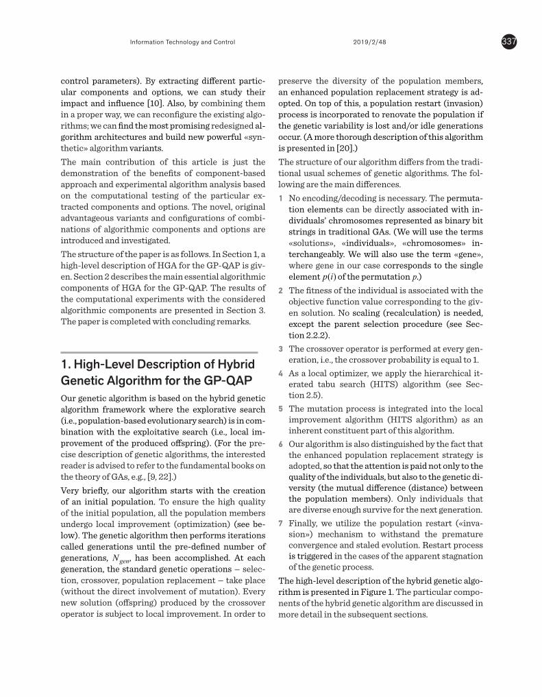
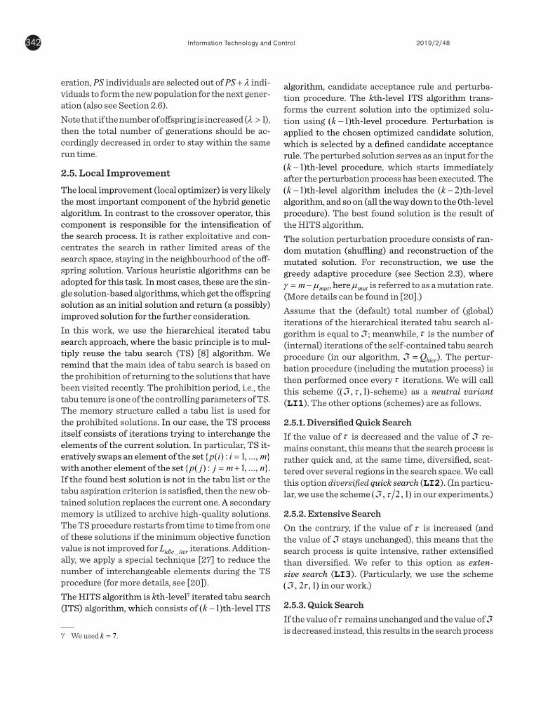
Figure 2 Examples of (pseudo-)optimal grey frames (n = 1024): (a) m = 300, (b) m = 301, (c) m = 302, (d) m = 303, (e) m = 304, (f ) m = 305, (g) m = 306, (h) m = 307

Figure 2. Examples of (pseudo-)optimal grey frames ( 1024n = ):

(a) 300m = , (b) 301m = , (c) 302m = , (d) 303m = , (e) 304m = , (f) 305m = , (g) 306m = , (h) 307m =

It is also shown that the local improvement process, along with the related numerical parameters, is indeed of the highest importance for HGA. The prolonged extensive improvement (more iterations of the improvement algorithm) is deemed to have greater potential as compared to the quick, concentrated improvement (less iterations of the improvement algorithm) for a fixed CPU time budget. The values of the parameters hierQ and τ should be carefully calibrated to achieve the best desirable effect (here, hierQ denotes the total number of iterations of the hierarchical improvement algorithm, τ is the number of the TS iterations). Overall, it is recommended that the value of the ratio

hier

gen

QN

(or genNτ ) be large enough (given that hier genQ N const⋅ = ), where genN is the number of generations of HGA. (For

example, 100hierQ = , 50genN = would be better than = 50hierQ , 100genN = .) We observed that the solution quality is more sensitive to the value of τ than hierQ (if other conditions remain unchanged). So, larger values of τ are recommended, especially if the problem size n is also large.

We notice that the problem-specific, tuned local optimizer should be adopted to save the computation time. More attention should be paid to the design and implementation of the population replacement component. It is

worth to try new non-traditional replacement schemes. Not only the fitness of the individuals is important, but also the distance between population members. The variability of the individuals of the population must be ensured.

As to the population restarts (invasions), we think that this aspect might have been in part underestimated by the researchers. In many GAs, the restarts are not used at all. But we believe that including restarts into the standard GAs has big potential. Only it is questionable what kind of restart techniques are more advantageous. So far, we have learned that adopting the "hot restarts" (for example, mild mutations applied to all population members) might be quite promising. The additional experiments are required to determine the most effective variants of the restart procedures. New types of restart techniques are needed. The attention should also be paid to the other factors linked to restarts, for example, restarts criteria and/or rates.

Overall, the conducted experiments exhibit that the quality of the obtained results is very encouraging. We report that, for one of the best designed component combinations — S3-C8-NOG3-LI3-PRS4 — the best known

solution was found at least 1 time out of 10 runs for every examined value of m for 256n = . On the whole, the BKV was found at least 1 time in 10 runs 183 times. In summary, the best known solution was

found 878 times. Our algorithm found the BKS in about 40% of the runs with 100m < . The newly designed algorithmic configurations achieved the BKS in nearly 85% of the cases with 100m < , while the particular variant S3-C1-NOG3-LI3-PRS4 found the BKS in 100% of these cases.

For 1024n = , the BKV was found at least 1 time in 10 runs 66 times. Overall, the best known value was achieved 455 times.

The average relative deviation from BKV for all tested values of m was only 0.048% for 256n = ; while the deviation for 1024n = was 0.166%.

For 256n = , we were able to find the best known solution in all 10 runs for 95, 96, 97, 98, 99m = . For 1024n = , we found the BKS at least once in 10 runs for 50, 70, 80, 120, 130m = . We found the BKS in all 10 runs for 50m = .

(a) (b) (c) (d)

(e) (f) (g) (h)

values of m was only 0.048% for 256n = ; while the de-viation for 1024n = was 0.166%.For 256n = , we were able to find the best known solution in all 10 runs for 95, 96, 97, 98, 99m = . For

1024n = , we found the BKS at least once in 10 runs for 50, 70, 80, 120, 130m = . We found the BKS in all 10

runs for 50m = .For the promising ensemble of options S3-C8-NOG4-LI3-PRS4, the average deviation never was larger than 0.027% for 256n = , while the cumulative average deviation of this ensemble for all 10 tested values of m is equal to 0.01% for 256n = . For our favourite as-semblage S3-C8-NOG3-LI3-PRS4, the deviation never was larger than 0.223% for 1024n = , while the cumu-lative deviation of this assemblage is equal to 0.06% for 1024n = .We used the configuration S3-C8-NOG3-LI3-PRS4 in additional extensive experiments with the large-sized problem instances ( = 1024n ). The enlarged size of the initial population was used. We also used the increased number of generations and increased number of iterations of the local optimizer (HITS al-gorithm). The number of runs of HGA was increased,


as well. During the experiments, we were successful to achieve new record solutions for 91 values of m. The results are reported in Table 11. The new BKVs are in bold face. All the remaining best known values are from [20]. It is very likely that with the greater run-time resources, the outcome may be improved with possibility of uncovering more best-known solutions.In Figure 2, we provide some graphical representa-tions (color frames) corresponding, in particular, to 300, 301, 302, 303, 304, 305, 306, 307m = . In the graphical illustrations, the 1024-square-grids are rep-licated 8 times horizontally and 8 times vertically for the visibility convenience. The squares’ color is blue (instead of black). The color code is #0000FF (in ac-cordance with the RGB color model), where "red" 0= , "green" 0= , "blue" 255= .

4. Concluding RemarksIn this paper, we present the results of the extensive computational experiments with the hybrid genetic algorithm for the grey pattern quadratic assignment problem. The experiments are based on analysing of various algorithmic features, i.e., components and their influence on the overall performance of HGA. The following essential components were examined: initial population, selection of parents, crossover procedures, number of offspring, local improvement, population replacement and population restart.

It has been ascertained that various components play different roles and they are not equally import-ant. The results of the computational experiments demonstrate the high importance of the initial pop-ulation and local improvement components. Starting from the improved initial population is indeed much more advantageous than using the random popula-tion. Overall, maintaining the superior-quality popu-lation is an essential aspect for HGA.Note that the aggressive, intensive local improvement of the offspring is preferable to fast, inexpensive local improvement; this is especially true for the large-sized problem instances. In these cases, the results obviously demonstrate the dominance of the local improvement (i.e., “exploitative”) component over “explorative” components (for example, crossover procedures).The experimental analysis indicates that it is of great importance to operate with highly diversified popula-tions and make use of the proper restart mechanism for avoiding the loss of genetic variability and the premature convergence of the genetic algorithm. The factor of the strength of restart of the stagnated popu-lation is very important.We emphasize that the large number of best known solutions were achieved for the GP-QAP instances of size 1024 by applying our found favourite configura-tion of the hybrid genetic algorithm.Our used methodology might be adapted for other types of heuristic algorithms. Also, it may be interest-ing to design an algorithmic framework for automatic configuring of the different components.

References1. Boussaïd, I., Lepagnot, J., Siarry, P. A Survey on Optimi-

zation Metaheuristics. Information Sciences, 2013, 237, 82-117. https://doi.org/10.1016/j.ins.2013.02.041

2. Çela, E. The Quadratic Assignment Problem: Theory and Algorithms, Kluwer, 1998. https://doi.org/10.1007/978-1-4757-2787-6

3. Drezner, Z. Compounded Genetic Algorithms for the Quadratic Assignment Problem. Operations Research Letters, 2005, 33(5), 475-480. https://doi.org/10.1016/j.orl.2004.11.001

4. Drezner, Z. Finding a Cluster of Points and the Grey Pattern Quadratic Assignment Problem. OR Spectrum,

2006, 28(3), 417-436. https://doi.org/10.1007/s00291-005-0010-7

5. Drezner, Z., Misevičius, A. Enhancing the Performance of Hybrid Genetic Algorithms by Differential Improve-ment. Computers & Operations Research, 2013, 40(4), 1038-1046. https://doi.org/10.1016/j.cor.2012.10.014

6. Drezner, Z., Misevičius, A., Palubeckis, G. Exact Algo-rithms for the Solution of the Grey Pattern Quadrat-ic Assignment Problem. Mathematical Methods of Operations Research, 2015, 82(1), 85-105. https://doi.org/10.1007/s00186-015-0505-1

7. Erkut, E. The Discrete p-Dispersion Problem. Europe-

https://doi.org/10.1016/j.ins.2013.02.041

https://doi.org/10.1007/978-1-4757-2787-6

https://doi.org/10.1007/978-1-4757-2787-6

https://doi.org/10.1016/j.orl.2004.11.001

https://doi.org/10.1016/j.orl.2004.11.001

https://doi.org/10.1007/s00291-005-0010-7

https://doi.org/10.1007/s00291-005-0010-7

https://doi.org/10.1016/j.cor.2012.10.014

https://doi.org/10.1007/s00186-015-0505-1

https://doi.org/10.1007/s00186-015-0505-1


an Journal of Operational Research, 1990, 46(1), 48-60. https://doi.org/10.1016/0377-2217(90)90297-O

8. Glover, F., Laguna, M. Tabu Search, Kluwer, 1997. https://doi.org/10.1007/978-1-4615-6089-0

9. Goldberg, D. E. Genetic Algorithms in Search, Optimiza-tion and Machine Learning, Addison-Wesley, 1989.

10. Hoos, H. H. Programming by Optimization. Commu-nications of the ACM, 2012, 55(2), 70-80. https://doi.org/10.1145/2076450.2076469

11. Kuby, M. J. Programming Models for Facility Dis-persion: The p-Dispersion and Maxisum Dispersion Problems. Geographical Analysis, 1987, 19(4), 315-329. https://doi.org/10.1111/j.1538-4632.1987.tb00133.x

12. Lim, M. H., Yuan, Y., Omatu, S. Efficient Genetic Algo-rithms Using Simple Genes Exchange Local Search Policy for the Quadratic Assignment Problem. Com-putational Optimization and Applications, 2000, 15(3), 249-268. https://doi.org/10.1023/A:1008743718053

13. Misevičius, A. Experiments with Hybrid Genetic Algo-rithm for the Grey Pattern Problem. Informatica, 2006, 17(2), 237-258.

14. Misevicius, A. Restart-Based Genetic Algorithm for the Quadratic Assignment Problem. In Research and De-velopment in Intelligent Systems XXV, Proceedings of AI-2008, the Twenty-eighth SGAI International Con-ference on Innovative Techniques and Applications of Artificial Intelligence, (Eds.) Bramer, M., Coenen, F., Petridis, M., Springer, 2008, 91-104. https://doi.org/10.1007/978-1-84882-171-2_7

15. Misevičius, A. Generation of Grey Patterns Using an Improved Genetic-Evolutionary Algorithm: Some New Results. Information Technology and Control, 2011, 40(4), 330-343. https://doi.org/10.5755/j01.itc.40.4.983

16. Misevičius, A., Guogis, E., Stanevičienė, E. Computa-tional Algorithmic Generation of High-Quality Colour Patterns. In Information and Software Technologies, 19th International Conference, ICIST 2013, (Eds.) Skersys, T., Butleris, R., Butkienė, R., Proceedings, Communications in Computer and Information Sci-ence (CCIS), 403, Springer, 2013, 285-296. https://doi.org/10.1007/978-3-642-41947-8_24

17. Misevičius, A., Kuznecovaitė, D. Investigating Some Strategies for Construction of Initial Populations in Genetic Algorithms. Computational Science and Tech-

niques, 2017, 5(1), 560-573. https://doi.org/10.15181/csat.v5i1.1277

18. Misevičius, A., Rubliauskas, D. Performance of Hybrid Genetic Algorithm for the Grey Pattern Problem. Infor-mation Technology and Control, 2005, 34(1), 15-24.

19. Misevičius, A., Rubliauskas, D. Testing of Hybrid Ge-netic Algorithms for Structured Quadratic Assignment Problems. Informatica, 2009, 20(2), 255-272.

20. Misevičius, A., Stanevičienė, E. A New Hybrid Genet-ic Algorithm for the Grey Pattern Quadratic Assign-ment Problem. Information Technology and Control, 2018, 47(3), 503-520. https://doi.org/10.5755/j01.itc.47.3.20728

21. Pavai, G., Geetha, T. V. A Survey on Crossover Operators. ACM Computing Surveys, 2017, 49(4), 1-43. https://doi.org/10.1145/3009966

22. Sivanandam, S. N., Deepa, S. N. Introduction to Genetic Algorithms, Springer, 2008.

23. Taillard, E. Comparison of Iterative Searches for the Quadratic Assignment Problem. Location Science, 1995, 3(2), 87-105. https://doi.org/10.1016/0966-8349(95)00008-6

24. Taillard, E., Gambardella, L. M. Adaptive Memories for the Quadratic Assignment Problem. Tech. Report ID-SIA-87-97, Lugano, Switzerland, 1997.

25. Talbi, E.-G., Hafidi, Z., Geib, J.-M. Parallel Tabu Search for Large Optimization Problems. In Meta-Heuris-tics: Advances and Trends in Local Search Paradigms for Optimization, (Eds.) Voß, S., Martello, S., Osman, I. H., Roucairol, C., Kluwer, 1998, 345-358. https://doi.org/10.1007/978-1-4615-5775-3_24

26. Tate, D. M., Smith, A. E. A Genetic Approach to the Quadratic Assignment Problem. Computers & Op-erations Research, 1995, 22(1), 73-83. https://doi.org/10.1016/0305-0548(93)E0020-T

27. Wu, Q., Hao, J.-K. A Hybrid Metaheuristic Method for the Maximum Diversity Problem. European Journal of Operational Research, 2013, 231(2), 452-464. https://doi.org/10.1016/j.ejor.2013.06.002

28. Zhou, Y., Hao, J.-K., Duval, B. Opposition-Based Memet-ic Search for the Maximum Diversity Problem. IEEE Transactions on Evolutionary Computation, 2017, 21(5), 731-745. https://doi.org/10.1109/TEVC.2017.2674800

https://doi.org/10.1016/0377-2217(90)90297-O

https://doi.org/10.1007/978-1-4615-6089-0

https://doi.org/10.1145/2076450.2076469

https://doi.org/10.1145/2076450.2076469

https://doi.org/10.1111/j.1538-4632.1987.tb00133.x

https://doi.org/10.1023/A:1008743718053

https://doi.org/10.1007/978-1-84882-171-2_7

https://doi.org/10.1007/978-1-84882-171-2_7

https://doi.org/10.5755/j01.itc.40.4.983

https://doi.org/10.1007/978-3-642-41947-8_24

https://doi.org/10.1007/978-3-642-41947-8_24

https://doi.org/10.15181/csat.v5i1.1277

https://doi.org/10.15181/csat.v5i1.1277



https://doi.org/10.1145/3009966

https://doi.org/10.1145/3009966

https://doi.org/10.1016/0966-8349(95)00008-6

https://doi.org/10.1016/0966-8349(95)00008-6

https://doi.org/10.1007/978-1-4615-5775-3_24

https://doi.org/10.1007/978-1-4615-5775-3_24

https://doi.org/10.1016/0305-0548(93)E0020-T

https://doi.org/10.1016/0305-0548(93)E0020-T

https://doi.org/10.1016/j.ejor.2013.06.002

https://doi.org/10.1016/j.ejor.2013.06.002

https://doi.org/10.1109/TEVC.2017.2674800

Documents

Experimental Analysis of Hybrid Genetic Algorithm for the