Experience Data Quality - Society of Actuaries

Experience Data QualityHow to Clean and Validate Your Data

Full Report

©2011, SOA and LL Global, Inc.SM | 3

Table of Contents Acknowledgement ........................................................................................................................................... 4

Introduction .................................................................................................................................................... 5

1. Relevance and Source of the Data ................................................................................................................. 7

2. Data Cleansing ............................................................................................................................................. 8

2.1 Causes of Data Errors .............................................................................................................................. 8

2.2 Defining Data Validity Errors ................................................................................................................... 9

2.2.1 Missing Value Errors ........................................................................................................................ 9

2.2.2 Data Format Errors ........................................................................................................................ 10

2.2.3 Coding Errors ................................................................................................................................ 10

2.3 Defining Data Accuracy Errors ............................................................................................................... 11

2.3.1 Experience Period Error ................................................................................................................. 11

2.3.2 Other Missing Value Error .............................................................................................................. 12

2.3.3 Relationship of Numeric Field Error ................................................................................................. 12

2.4 Detection Techniques ........................................................................................................................... 13

2.4.1 Automation ................................................................................................................................... 13

2.4.2 100 Records .................................................................................................................................. 13

2.4.3 Frequency Distribution .................................................................................................................. 14

2.4.4 Sampling ....................................................................................................................................... 15

2.5 Solutions.............................................................................................................................................. 16

2.5.1 Deleting ........................................................................................................................................ 16

2.5.2 Ignoring ........................................................................................................................................ 17

2.5.3 Correcting ..................................................................................................................................... 17

2.5.4 Filling In ........................................................................................................................................ 18

3. Data Validation .......................................................................................................................................... 19

3.1 Data Consistency .................................................................................................................................. 19

3.1.1 Time Horizon ................................................................................................................................. 19

3.1.2 Inconsistency ................................................................................................................................ 19

3.1.3 Longitudinal .................................................................................................................................. 21

3.2. Data Reasonability ............................................................................................................................... 21

3.3 Data Completeness and Credibility ........................................................................................................ 22

Appendix – Sampling Methods........................................................................................................................ 23

Data Quality Software .................................................................................................................................... 30

Glossary ........................................................................................................................................................ 31

Bibliography .................................................................................................................................................. 32


Acknowledgement

LIMRA and the Society of Actuaries (SOA) extend their gratitude to the members of the Project

Oversight Group (POG) for their input and review throughout this project.

Representing LIMRA Representing the Society of Actuaries

Danielle Brancard Bud Ruth, Chair, Project Oversight Group

Cathy Ho Sharon S. Brody

Elaine Tumicki JJ Lane Carroll

Susan Deakins

John Have

Kevin Pledge

Peter Weber

Ronora Stryker, SOA Research Actuary

Jan Schuh, SOA Sr. Research Administrator

The report was primarily authored by Cathy Ho and Danielle Brancard with assistance and input from

the Project Oversight Group. The opinions and views expressed and conclusions reached by the authors

are their own and do not represent any official position or opinion of the Project Oversight Group

members or their employers, Society of Actuaries or its members, and LIMRA or its members.


Introduction

In the current economic environment, having high quality data is essential for a competitive edge. Poor

quality data is an issue in all industries. The Data Warehouse Institute estimated that data quality

problems cost U.S. businesses over $600 billion a year. Specifically for life insurers, the quality of data

used in experience studies is the primary focus of this paper. Industry experience studies are resources

life insurers use to manage and monitor their blocks of businesses. However, current voluntary

submissions to the Individual Life Experience Committee of the SOA (ILEC) annual experience study data

calls continue to be inconsistent. This leads to delays, reduced analysis, and possible data compromises

in the reported results. With the principle-based reserving approach of the NAIC , it is likely that

mandatory experience reporting will be required. Unlike the ILEC data submissions, the responsibility

for high quality data in the NAIC data submissions will be on the life insurers.

The purpose of this paper is to provide an overview of the data cleansing and validation role specific to

the life insurance experience study process. Very little has been written about data cleansing and

validation specifically for data used in the life insurance experience study. Discussions in this paper will

include common data errors, likely causes of these errors, methods for detecting these errors, and

possible solutions. While the examples and techniques are focused on life insurance, most can be easily

translated for use with other insurance products. This can be used as reference material for actuaries

and analysts involved in experience studies.

It is first important to understand the impact of poor data quality and the value of good quality data.

Data quality problems specific to the experience study process are harder to measure. Using inaccurate

experience results could lead to bad pricing and product design, which leads directly to profitability risk

and possible capital and surplus strain. This could also lead to reserve adequacy issues down the road.

For many companies, a significant decline in sales due to over pricing could lead to solvency issues.

Figure 1: Implications of Poor Quality Experience Data

Poor Quality Experience Data

Inaccurate Experience Study Results

Risk to Profitability

Antiselection Risk

Inappropriate Reinsurance

Risk to Capital & Surplus

Reserve Adequacy Risk

Risk to Company Rating


While mispricing can be seen immediately through sales results, other consequences of poor experience

data occur much later. For example, different aspects of valuation such as risk based capital, DAC, and

tax reserves depend heavily on experience projections. Using inaccurate experience study results for

these projections could lead to considerable changes in reserves, decline in capital and surplus, and

possible downgrades to the company’s financial ratings. Misunderstanding or not knowing the true

experience of a block of business can also lead to inappropriate reinsurance decisions.

It is because of the seriousness of these implications that the role of data cleansing and validation is vital

to the life insurance experience study process. And because of the magnitude of the costs due to data

quality problems, several data management and data quality tools exist in the current marketplace.

While many of these data management and data quality tools have the ability to provide high quality

data in general, they are not as well suited to life insurance experience study data. This is mainly due to

the uniqueness of experience study data, with wide variations in acceptable values and outliers.

One tool that has been created specifically for use with life insurance experience study data is the SOA

Data Quality Tool. The SOA Data Quality Tool software was created to specifically detect many of the

common data errors found in experience studies, described in later sections. It also provides different

views of the data to allow a knowledgeable analyst to visually detect the more complex errors.

However, this tool is limited to the data collected utilizing the VM-51 format.

Software of any kind should be considered an aid to data cleansing and validation. It is not meant to be

a replacement for analysts and actuaries. Whether a system is purchased or built in-house, the need

for a well trained and knowledgeable analyst or actuary to review the data is crucial.


1. Relevance and Source of the Data

The first steps to quality data are to know the source of the data and how the data will be used. Data

source is particularly important with inter/intra-company studies as data formats are more likely to vary

from source to source. Because a poor quality data source will require more time and resources to

resolve data issues, creating and using a good quality source should be the primary goal. When data

errors are found to be contained within the data source, it is generally recommended that corrections

be made to the data source. However, corporate guidelines should take precedence as there may be

other parties who feel that the source admin systems should be the system of record even, if the data is

incorrect. Because of this, other options are discussed in later chapters and sections.

The relevance of the data is equally important. Time and resources spent compiling the data and

resolving data issues would have been wasted if the data were not used for the experience study. An

example would be collecting premium payment patterns for a standard mortality study. While premium

payment pattern data would be beneficial in a universal life premium persistency study, it is not likely to

be used in a mortality study. In addition to unused data fields, there is also the possibility that the

results of the entire study are obsolete or outdated. Special attention should be given to the time

horizon of the experience data as well as the time frame of the data cleansing, validation and analysis.


2. Data Cleansing

The objective of data cleansing is to have valid and accurate data. Data validity is the foundation for

data cleansing and validation. Without valid data, all other data cleansing and validation would be a

waste of time. For example, if a house is constructed on a deficient concrete slab, at some point the

foundation will crumble causing the construction to collapse. The same is true for this first and most

basic step in data cleansing – data validity.

Data validity checks are needed to provide a solid basis for all other data cleansing and validation

checks. While it is possible to detect data validity errors within other aspects of data cleansing and

validation, the time and effort are better spent focused on finding and correcting common data validity

errors first before moving on to more complex data checks. However, before digging into definitions

and examples of data validity and accuracy errors, it is helpful to understand how some errors come

about.

2.1 Causes of Data Errors

Data validity errors are more common and widespread than data accuracy errors. They are also more

frequent in inter/intra-company studies. Both of these types of errors can occur in all records

throughout the data for a specific field (field error) or for certain records in specific fields (value error).

In many instances, they are caused by data entry errors when policy information is initially entered into

the source data. In other instances, a specific data field may not have been stored in the source data or

was lost during system migrations. Another common cause is that the error occurred when collecting

the data from the source data.

Frequently, data entry error is to blame for the data validity and accuracy errors within the source data.

For many companies with legacy systems, some fields were never collected initially, entered incorrectly,

or were lost or changed during system migrations. The occasional data entry errors will likely produce

errors with a random pattern, while the other causes will likely produce errors in blocks of records or a

number of consecutive records.

Other incidences of data validity and accuracy errors occur during data compiling, when the wrong field

is pulled out of the source data. An example of this would be pulling a character field from the system

to use as a numeric field within the experience data. While the character field may contain accurate

data, translating them into a numeric value may leave a significant portion of records with errors.

Because of the numerous fields within most data sources and experience study data, it is easy to mix up

the necessary fields and the order of the fields. This cause is especially common in inter/intra-company

studies where multiple data sources are used. Even for intra-company studies, it is unlikely that data

sources are identical. Multiple data sources increase the chances of data validity and accuracy errors

caused when collecting data for the experience study.

With understanding of various causes of data errors, the first step in data cleansing is to identify the

errors within the policy data. Sections 2.2 and 2.3 define data validity and data accuracy errors,


respectively. Once the errors are defined and understood, section 2.4 discusses various techniques to

identify these errors within the policy data.

2.2 Defining Data Validity Errors

As stated before, data validity errors are more common and widespread than data accuracy errors.

Three general types of data validity errors are discussed in the subsections below: missing value, data

format, and coding errors.

2.2.1 Missing Value Errors

Depending on the specific field, end result analysis, and the programming for the analysis, some fields

will have legitimate missing values. These are not considered invalid data and are ignored in this paper.

Before attempting to find the missing value errors, it is important to understand what is considered an

error within the data. The first step is to understand how the analysis programs are set up. For

example, can the program handle a blank/null value in a numeric, character, and date field? If no, then

all missing field values are considered errors.

The example below focuses on the gender field. Depending on the circumstances, a blank/null value

could be a valid value. For example, unisex policies may not be coded in this field. However, the analyst

must be aware that the missing values may lead to an issue if the results are to be compared with only

male and female mortality experience tables.

If the programming can handle blank/null values, then the next step is to identify and list which fields

should not have missing values, in some cases listing fields that are allowed missing values could result

in a shorter list. To create this missing field list, one must have knowledge of what analysis will be done

in the study. At a minimum, the basic info about the insured is required. This would include fields such

as policy number or unique identifying number, date of birth, gender, and face amount. In addition

other fields should be added to the list if they are to be included in the experience study. For example,

the issue date field should be added to the list if analysis of experience by issue age is planned. If

experience by underwriting type is desired then the underwriting type field should be included within

the list.


The fields mentioned so far are standard to most policies. There are fields tied to specific policies that

may have legitimate missing values for a good portion of the data. These missing value errors are

typically contingent on other fields. It is not recommended that these be added to the missing value

field list as it would likely mean more time shifting through the legitimate missing values than finding

missing value errors. These types of errors are discussed in the data accuracy section.

2.2.2 Data Format Errors

The first step in understanding data format errors is to know the source data and what is to be collected

for the experience study. Oftentimes, variations within different data sources can cause problems.

These errors can also easily occur during system migrations or conversions. For example, data source 1

may store a field as a numeric while data source 2 uses a character or string format for the same field.

Combining the two for the experience study would cause a data format error due to the inconsistency.

This situation can also occur for fields containing both numeric and character values.

With string and character formats, a value of 1 is not necessarily the same as a value of 01. But with a

numeric format, both values would be equivalent. These discrepancies become a setback during the

analysis phase and are better off processed during the early data cleansing phase.

Another common data format error is with date fields, such as date of birth, issue date, and termination

date. Different data sources may use different variations of date formats from one another, making it

difficult to compile experience data by month or year. Using consistent date formats, like DD-MM-YY or

MM-DD-YY, for example, would eliminate the discrepancies. There is also a preference to using the

YYYYMMDD as it can be more effortlessly sorted numerically.

2.2.3 Coding Errors

Coding errors, also called mapping or translation errors, occur when a field value is not an accepted

value for the field. The definition encompasses missing value and data format errors. However, since the

paper has addressed these errors already , this section will focus on other coding errors.

The common example is that a field is defined to have a number of stated values, but contain more than

those values. The gender field is defined as 1, 2, and 3 for male, female, and unisex. Any values other

than 1, 2, or 3 would constitute coding errors.

Taking the prior example from data format errors, for the two-character field the values ‘1 ’, ‘ 1’, and

‘01’ are considered different values. The first value contains a ‘1’ followed by a blank space, while the

second value starts with a blank space followed by ‘1’. The third value uses ‘0’ to fill in the blank space

before the ‘1’. It may be the case that only ‘ 1’ (blank space followed by ‘1’) is an acceptable value for

this field. This is not considered a data format error because the field is defined as a two-character field

and values within the field are two characters. However, this is a coding error because not all values

within this field are accepted values.


There are also more complex coding errors that involve more than one field. In the case of termination

date, the error is tied to whether or not the policy is terminated. If the policy is inforce, a date value

within the termination date field is considered a coding error. Depending on how the analysis program is

set up, acceptable values may be a blank or a pre-assigned value to denote a blank.

Coding errors also occur in date fields. Incorrect dates such as 9/31 or 2/29 (in a non-leap year) are

considered coding errors. Depending on the type of software used in the source and data compiling, this

may be easily detected.

2.3 Defining Data Accuracy Errors

Even if data pass the data validity error checks, it is still possible to have inaccurate data. A thorough

data cleansing includes both data validity and data accuracy checks. Data accuracy in this context

relates to data errors outside of data validity errors. This step essentially goes over the data with a “fine-

toothed comb”. While it is possible to find data validity errors in this step, the process is not

recommended due to the additional time and resources needed for data accuracy checks.

Data inaccuracies are more complicated than invalid data but are also less frequent; however, it does

require more knowledge of the data and how the data will be used. Examples of common accuracy

errors include experience period error, other missing value errors, and relationship of numeric field

errors, described below.

2.3.1 Experience Period Error

One common error is data outside of the experience period. While the records may contain valid data,

any policy not within the experience period is considered inaccurate. This includes policies issued after

the experience period and terminations not within the experience period. For example, if the

experience study is for 2009-2010, all policies issued after 2010, terminated before 2009, and

terminated after 2010 are considered errors.


A subset of this error is with observation years and when each inforce policy has a record for each

observation year. Using the prior example, records with an observation year of 2009 should not contain

policies with issue year 2010 or termination date in 2010.

2.3.2 Other Missing Value Error

For missing value errors, a list of identified fields that should not have missing values should have been

created (see section 2.2.1.). For those not on this list, some records with missing values are considered

data accuracy errors. A common error is the policy status and additional termination information that

are necessary for experience studies. Fields used for additional termination information contain

legitimate missing values. A termination date is expected only for terminated policies, whereas inforce

policies will have legitimate missing values for termination date. Therefore, only terminated policies

should be checked for missing values in this field. Possible solutions for this error are discussed in

section 3.5, a specific solution for this is discussed in example 2 of section 3.5.4.

Another example of this is the death benefit option field. This field is used only for universal and

variable universal life policies and will have legitimate missing values for term and whole life policies. If

most of the policies are UL or VUL, then it is more beneficial to add this field within the missing value

field list.

2.3.3 Relationship of Numeric Field Error

Many of the numeric fields in the experience data have ties to other numeric fields, much like

observation year, experience year, issue year, and termination year within the experience period error.

Other examples of these types of errors are listed below.

Example 1: Face amount and cash value. Within individual life experience data, the cash value

of a policy should always be less than the face amount of the policy.

Example 2: Face amount and premium. Similar to Example 1, the premium paid at any one

point or in total should always be less than the face amount of the policy.


Example 3: Issue age and attained age. Issue age should normally be less than or equal to

attained age.

2.4 Detection Techniques

There are several ways to find valid data errors. The main constraints are time and resources in

exchange for a higher portion of valid data. With the advanced computing power that is widely

available, more detection and corrections can be automated. Automation can greatly reduce the

analyst’s time constraints. For larger volumes of data, hardware computing time and resources could

become significant. This is unlikely to be an issue for most companies, but inter/intra-company studies

with tens or hundreds of millions of records could take hours to pick through.

2.4.1 Automation

Automating the detection of valid data errors is

straightforward. It is time consuming to initialize, but once

completed only minimal maintenance is needed. For each

field on the list, programming may be put in place to detect

valid data errors and apply solutions. The solutions should

be manually approved prior to automation.

In cases where data fields being used for the experience study are uncertain and changing, it may not be

worth the time and effort to program automated checks. This situation would have to depend solely on

techniques with an analyst’s review. Whether the automated program is minimal or thorough, an

analyst should still review the data.

2.4.2 100 Records

One of the simplest techniques is to grab 100 consecutive records and visually inspect them for errors.

This is the quickest and easiest way to detect valid data errors where an entire field is incorrect. This

approach also uses consecutive records to more efficiently detect block errors. While this is a very

effective technique in detecting large scale errors and errors within the 100 records, it is not an effective

technique at detection errors within the data as a whole.

An example of this would be policies issued in 1990 with an administrative system that did not retain

each policy’s distribution channel. Unless the data were sorted, this block of business was added to the

experience data together and consecutive records will have missing values in the distribution channel

field. The number of records is somewhat arbitrary. A smaller set is likely to miss blocks of records with

similar errors, while a larger set could become difficult for the analyst to review.


This method’s starting point can be chosen arbitrarily. In some cases it may be beneficial to have

additional filters. With the previous example, because of the extra information stored on separate

accounts for variable universal life policies, data were incorrectly collected for annual premium, causing

the null values within this field. Reviewing the 100 records may show a few records with missing values

in the annual premium field. However, filtering for only variable universal life policies, it becomes clear

that this is a widespread error.

This is a very effective technique in detecting errors within the 100 records; however, it is not an

effective technique at detecting errors within the data set as a whole. This technique must be repeated

several times, depending on the size of the data set, to be truly effective, but quickly becomes time

consuming. Even with several iterations, the probability of finding random data entry errors is low.

There is also the added probability of human error when reviewing the 100 records with each iteration.

2.4.3 Frequency Distribution

For reasonable sized data sets, the use of frequency tables,

whether this is a straight numeric table or graphed, is a

practical and thorough approach. Running a summary report

of record counts by field values allows for a relatively quick

visual check for valid data errors. Note that these reports are

fairly uncomplicated for fields with discrete and limited values.

An example of such a field is gender, where the number of

distinct values is likely under 10.

But for fields with indiscrete or limitless values, such as face

amount and premium, a basic frequency table would be

cumbersome. For these types of fields, bands and ranges are

recommended for quicker error detection.

The frequency table technique can also be used with larger volume data and inter/intra-company

studies; however, the analyst must weigh the trade-off between precision versus time and resources.


2.4.4 Sampling

For larger volume data, an alternative method is to apply detecting techniques to a sample of the

experience data. This technique can also be applied to a smaller volume of data, but is unlikely to

increase the percentage of valid data for the additional time and resources spent. Appropriate sample

size and sampling techniques are described in more detail in the Appendix section. Sampling methods

discussed in the appendix include simple random sampling, stratification, systemic and cluster sampling.

For individual company studies, sampling within categories should be considered. The most

fundamental categorization is by product. Whether it’s a simple two category split of term and

permanent products or categorized by each individual product is up to the analyst. Keep in mind that

the greater the number of categories, the higher the probability of error detection — but also the

greater the use of resources and time.

Sampling: Intra-Company For intra-company studies, a similar decision must be made on how to

sample. Sampling categories based on company should be considered for intra-company studies when

there are multiple data sources, data of each subsidiary company is a reasonable size, and where some

subsidiaries are closed blocks of business or purchased blocks. Categorizing by company allows the

analyst to focus on one block of business at a time. This becomes particularly important when detecting

other errors because more knowledge and understanding of the data is necessary.

In cases where subsidiary data are relatively small, categorizing by company is not recommended. This

runs into the constraints trade-off with using sampling for smaller individual company data.

Sampling: Inter-Company Because of the variance in experience by company, it is vital to

categorize by company, along with other subcategories, for inter-company studies. Inter-company

experience data should rarely be treated as a whole for data cleansing and validation. Instead, each

company’s experience data should be cleansed and validated separately. This is also due to the

differences in data source and data submission. The techniques mentioned above are all applicable. For

larger volume data, sampling should be considered.

It may be argued that in this case the law of large numbers allows for a lesser percentage of valid data.

However, the implications and use of the results should be heavily weighted when allocating resources

to data validation and cleansing.

After identifying the appropriate records, a decision must be made whether to delete the records from

the data, correct the error, or make other adjustments. In certain cases, correcting the error may not be

feasible. However, for smaller data sets, removing the records from the policy data set may be an issue

for the experience study in terms of credibility, exposure, and depth of analysis. In these situations,

alternative solutions may be more suitable than removing the records. Solutions and examples are

discussed in the next section.


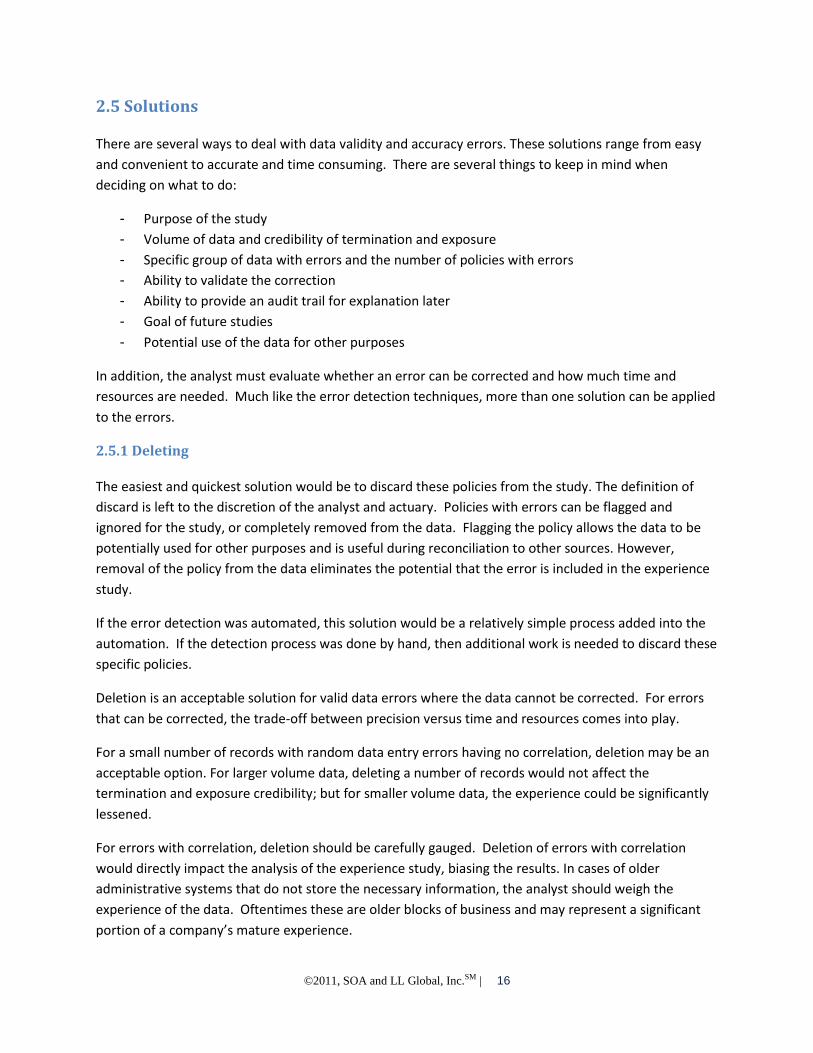
2.5 Solutions

There are several ways to deal with data validity and accuracy errors. These solutions range from easy

and convenient to accurate and time consuming. There are several things to keep in mind when

deciding on what to do:

- Purpose of the study

- Volume of data and credibility of termination and exposure

- Specific group of data with errors and the number of policies with errors

- Ability to validate the correction

- Ability to provide an audit trail for explanation later

- Goal of future studies

- Potential use of the data for other purposes

In addition, the analyst must evaluate whether an error can be corrected and how much time and

resources are needed. Much like the error detection techniques, more than one solution can be applied

to the errors.

2.5.1 Deleting

The easiest and quickest solution would be to discard these policies from the study. The definition of

discard is left to the discretion of the analyst and actuary. Policies with errors can be flagged and

ignored for the study, or completely removed from the data. Flagging the policy allows the data to be

potentially used for other purposes and is useful during reconciliation to other sources. However,

removal of the policy from the data eliminates the potential that the error is included in the experience

study.

If the error detection was automated, this solution would be a relatively simple process added into the

automation. If the detection process was done by hand, then additional work is needed to discard these

specific policies.

Deletion is an acceptable solution for valid data errors where the data cannot be corrected. For errors

that can be corrected, the trade-off between precision versus time and resources comes into play.

For a small number of records with random data entry errors having no correlation, deletion may be an

acceptable option. For larger volume data, deleting a number of records would not affect the

termination and exposure credibility; but for smaller volume data, the experience could be significantly

lessened.

For errors with correlation, deletion should be carefully gauged. Deletion of errors with correlation

would directly impact the analysis of the experience study, biasing the results. In cases of older

administrative systems that do not store the necessary information, the analyst should weigh the

experience of the data. Oftentimes these are older blocks of business and may represent a significant

portion of a company’s mature experience.


2.5.2 Ignoring

An alternative to deletion is to ignore the error. This is just as easy and quick of a solution as deletion;

however, more hands-on review and analysis is required before implementing. Unlike deletion where

the entire policy would be discarded, this approach keeps the policy in place but ignores the specific

field of the policy. Instead of looking at groups of records with similar errors, this approach looks at the

number of errors within each record. If a record contains only one error, it may be worthwhile to use

the ignoring approach rather than deleting. As with deleting, termination and exposure credibility is still

an issue when applying this technique over correcting the error.

If analysis is planned for the smoker status field and several records have a missing value only for this

field, it would be valuable to keep these records and ignore the error for smoker status. These policies

will still contribute to the overall experience and other analysis. Additionally, the missing value can be

- Left blank - noting that these errors are accepted

- Replaced with a value not reflective of the field

- Flagged to be ignored for specific analysis

If smoker status includes the values 1 through 5 and the replacement approach is selected, a value

should be chosen outside of the range so that these policies are not accidently included in the smoker

analysis.

For records with few errors, ignoring those errors may benefit the overall study — although errors

within critical fields should not be considered for this technique. Including records with missing

termination status and ignoring the error would add no benefit to an experience study. Records with

missing ages would be of little use for a mortality study but can still be beneficial in a lapse study.

For inter/intra-company studies and individual company studies where credibility is less of a concern,

this solution is favored over deletion.

2.5.3 Correcting

The most precise and preferred technique is to correct the data. Some valid data errors are fairly simple

and quick to correct. The most common of these tend to be errors that occur when compiling the data,

such as grabbing incorrect fields or putting the fields in the wrong order.

Other common errors occur when dealing with multiple data sources and having to translate field values

to a common value. For example, the gender field in admin system 1 is coded (M, F, U) while admin

system 2 is assumed to be coded (male, female, unisex). However, admin system 2 also has codes

(unisex-male, unisex-female). If these two codes were not anticipated, then the gender fields for these

records are likely blanks.


2.5.4 Filling In

In some cases the error comes from the source and cannot be fixed. Rather than deleting or ignoring

the error, another alternative is to try to decipher the true value by using other valid fields for the

policy.

Example 1: The error is in the smoker status field. If the nonsmoker preferred class contains

valid data, it can be implied that the policy has nonsmoker status.

Example 2: The error is a missing termination date for a terminated policy. The premium

paid-to-date can be a reasonable substitute.

These examples are straightforward, but others may not be. It is recommended that an analyst with

knowledge of the data use this technique rather than automating.


3. Data Validation

Data validation detects potential data errors not easily found in the data cleansing step and also

assesses the soundness of the experience data as well as the study results. Data cleansing and data

validation go hand in hand. If data cleansing is considered the foundation of a house, then data

validation would be considered the framework of the house. It is possible to build a house without a

foundation, but the result would be questionable. And without a framework, it would be difficult to

build a house. The same is true for data cleansing and data validation. It is possible to omit data

cleansing and go straight to data validation. The errors are likely to show up during the analysis phase.

Omitting the data validation, on the other hand, is likely to produce questionable experience study

results.

This chapter describes the three common phases of data validation: consistency, reasonability, and

completeness.

3.1 Data Consistency

While data for other business may fluctuate significantly over different time periods, most data used for

experience studies should be fairly consistent from study to study. This section discusses the

appropriate time horizons, ways to compare the data to gauge data consistency, and longitudinal

consistency.

3.1.1 Time Horizon

The time span chosen for the experience study depends mainly on the goals of the study. If the main

goal of the study is to continuously trend lapse experience, one full policy year or two consecutive

calendar years of data may be appropriate. In this case, products influenced by economic conditions

can be easily seen in the trends. However, if the goal is to compare mortality experience to industry

tables, then a greater time horizon would be more suitable.

The same applies to the frequency and timeliness of experience studies. For lapse (and possibly

mortality) experience of new and rapidly selling products, annual or biennial studies when data becomes

available is more applicable. When the goal is to compare original pricing assumptions to actual

experience on a block of business, longer time periods with less frequent studies are suitable. Especially

for shorter time horizons, the analyst must also keep in mind the volume of data.

3.1.2 Inconsistency

With the time horizon set, the next step is to gauge data consistency. There are several reasons data

inconsistency would occur. The most common cause is incorrect data. While the data may have passed

the data cleansing phase, it is still possible that certain records are incorrect. A simple example of this is

when analyzing a specific block of business or a particular subsidiary. Inconsistency in the data


compared with prior studies may indicate the wrong block of business or subsidiary. On the other hand,

inconsistency could also signal changes in products and business plan.

In general, comparison should be made of the year-over-year change in the number of policies, face

amount, and premium. Percentage change should be small, less than ±5%, unless there is reasonable

cause. This is due to the greater portion of mature business consistency between studies, with the small

changes due to termination offsetting new sales. A larger percentage increase may be an indicator that

inappropriate data have been included while a larger percentage decrease could indicate data are

missing from the study. Reasonable causes for a larger percentage change range include a new product

gaining market share, a change in business strategy, or a sell-off of a block of business. The lack of

change may also be indicative of an issue.

Below are some examples of varying levels of comparison. Each can be used on its own or combined

with others.

1. Overall Totals The most basic method is to compare data totals between studies. This

method is quick and simple, but not thorough.

a. If the data is a closed block of business then the totals should decline from study to

study due to terminations. Increases would signal incorrect data.

b. For younger companies with less mature experience, a greater percentage of fluctuation

is expected. In this case, it is difficult to tell whether the inconsistency is natural or due

to error.

c. For inter/intra-company studies, this level of comparison should be used only when

there is consistency in participating companies from study to study.

2. By Product This method requires more knowledge of the data by product line. Whether this

is split by the main product lines (whole life, term, universal life, & variable life) or a more

detailed split (10-yr term, 20-yr term, etc.), the analyst must be familiar with what is happening

and what has happened to the business. This finer split also allows for better detection of

incorrect data.

a. A larger decline in whole life offsetting a larger increase in term may show consistency

with overall totals comparison. However, a comparison by product line will tell a

different story.

b. Similar to the overall totals comparison, a discontinued product should trend a decline

from study to study, while a newer product will show greater fluctuation.

3. By Observation Year In addition to comparing consistency between studies, it is also

recommended that comparison be done within the current study when possible. For studies

with a time horizon of more than one year, there should be consistency between observation

years.

4. By Company For inter/intra-company studies, it is recommended that comparisons are done

at the company level, due to the large volume of data. In addition, errors are more likely to hide

within inter-company studies where contributing companies vary from study to study. Breaking

out the comparison by company reduces the chances of such errors.


3.1.3 Longitudinal

Longitudinal data inconsistencies are more likely to occur in experience studies with longer time

horizons or when shorter time horizon studies are compiled across time, as is true for the inter-company

mortality study. These inconsistency errors can occur when changes are made to policies.

An example of this would be if a policy was reported as a death in late 2008, but was then reinstated

two months later in 2009 as a false claim. Mortality study for experience year 2008 would show the

policy has a claim; however, the mortality study for experience year 2009 would credit the policy as

inforce. When the two studies were compiled into a larger mortality experience study, this specific

policy would create a longitudinal data consistency error.

This type of error can be potentially time and resource consuming, particularly for inter/intra-company

studies with large volumes of data to sift through. There are no simple techniques to detect these

errors, but robust computer programming can flag potential policies with these errors. In cases where

policy record identifiers are consistent, data sets can be merged and mapped through programming to

eliminate errors. As with the other data errors, a knowledgeable analyst or actuary is necessary.

3.2. Data Reasonability

In some cases, it is hard to detect a data issue until the analysis begins. This is particularly true for larger

volume of data such as inter/intra-company studies. Data reasonability refers to the reasonability of the

data based on the experience results. As with data consistency, experience results should be expected

to be somewhat consistent from study to study. Trends can form over time. Similar to data consistency,

a comparison of the results from study to study will highlight potential data issues.

The most likely causes of reasonability errors are policies missing from the data, the data contain

policies not within the scope of the experience study, and miscoded fields. The latter refers to

miscoding, such as a policy coded as simplified issue when it should be a non-medical underwriting

policy.

1. Unexpected Spikes Unexpected spikes in experience results are usually a good indicator of

possible data issues. When results are graphed, these can be easily detected as the anomalies

along a smoother trend. There are few expected spikes within experience results; the most

common example would be shock lapse rates at the end of level premium term periods.

2. Change in Experience Any notable changes in experience should be analyzed in more

detail. While an improvement in mortality is expected, a significant improvement may indicate

potential issues in the termination cause field, unreported deaths, or missing terminated

policies. There are cases where significant changes are due to changes in business strategy,

such as the introduction of a policy retention program.

3. Change in Trend Shifts in trends are also a good indicator of possible data issues. First year

lapse rates for whole life are typically the highest among all policy years. If results show that

third year lapse rates exceed first year lapse rates, there could be a potential issue for whole life

policies in the first duration and third duration.


4. Trends in Data Trends in particular parts of the data can also be an indicator of data issues.

Specifically watch for fewer terminations near the end of the experience period. This may

indicate late reporting and perhaps the data was extracted too soon.

As with other data errors, the analyst must make a decision whether to remove, ignore, or correct the

data. In some cases it is difficult and time consuming to correct the data. Removing or ignoring may be

the most efficient solution. However, the issues of data completeness and credibility become more likely

problems.

3.3 Data Completeness and Credibility

Data completeness and data credibility go hand in hand where data completeness refers to the amount of accurate and available data for use in the experience analysis and data credibility refers to the data’s ability to provide reliable and trustworthy results. A greater degree of data completeness implies the opportunity for a more extensive analysis of the experience results, as well as greater credibility. When applying solutions for data errors, the analyst should always keep this issue in mind. While it is easier to remove or ignore the error, not spending the time to correct a correctable error could lead to loss of analysis.

The problem with data completeness is a greater issue for inter/intra-company studies. Some data sets may not contain all required fields. In this case, a decision must be made whether to exclude various company experiences from particular results or remove the analysis altogether. A similar time and resource trade-off exists, but due to the voluntary nature of inter-company studies it is more difficult to acquire data corrections. On the other hand, because of the larger volume of data, there is less worry about credibility with inter-company studies.

Determining the level of data completeness is solely up to the actuary or analyst. Credibility for

individual company and intra-company data however should be estimated with inter-company studies.

For additional information about credibility please refer to: http://www.soa.org/research/research-

projects/life-insurance/research-credibility-theory-pract.aspx

http://www.soa.org/research/research-projects/life-insurance/research-credibility-theory-pract.aspx

http://www.soa.org/research/research-projects/life-insurance/research-credibility-theory-pract.aspx


Appendix – Sampling Methods

How long would it take to carefully look through 4 million records and analyze the data? It is

probably possible, yet, time consuming. This is when sampling methods come into play. While the

amount of data is reduced, rather than a full population, analysts will want the data to be reflective of

the full population being sampled so accurate analyses can be made. Random samples give a better

representation of the population because every object or person, in a specific sampling frame, is given

an equal opportunity to be picked for the subset. Analysts can also apply their conclusions from what

they discover about the sample data to the whole population. It is vital that data are not biased in the

subset, as making an analysis about the full population is what is intended.

The following sampling techniques will allow the sample to represent the population: simple random

sampling, systematic sampling, stratified random sampling, and cluster sampling. However, one may be

more effective or efficient than another—their results differ from case to case. Additionally, there are

advantages and disadvantages to each of these methods.

A.1 Simple Random Sampling

Simple random sampling is the most straightforward method used in which every entity of the

population has an equal chance to be selected for the sample. Data probably are easiest to collect in

this method, but the steps need to be carefully followed because data can become erroneous very

easily.

A.1.1 How to Gather the Data

An effective technique is a random number generator. Each entity of the population would be

assigned a number while the random number generator would produce n numbers, where n equals the

proper sample size associated with the sampling frame. For instance, if the data contain 100 records,

records should be assigned numbers from 1 to 100. The random number generator should then

generate the appropriate set of different random numbers. The numbers randomly picked should be

matched up with the records that are assigned, and those are the records that will be used in the

sample.

Additionally, many programming systems have random number generators, such as Excel, SAS,

SPSS, Minitab, C++, and Java, to name a few. In fact, several of these systems have simple random

sampling functions built in. Ho and Brancard used SAS programs for many of their calculations.

Before an analyst can begin a simple random sample (SRS) an effective sample size needs to be

determined. The analyst must first determine an appropriate margin of error and confidence level, and

then calculate the sample size by using other variables including the population size, proportion, and a z-

score.


A.1.2 Assigning Variables

The margin of error and confidence level are very important because they help determine the

measure of precision for a sample size. The most common margin of error used is 5 percent; however,

anything less can be used. The most typical choices for a confidence level are 95% and 99%. The 95%

confidence level is most commonly used — although a 99% confidence level will provide higher

precision. Confidence levels between 95% and 99% can also be used. The reason why a larger

confidence level is more commonly used is because the results are not far off from the true answer, or

what would be determined from the whole population. A lower margin of error and a higher confidence

level necessitate a large sample size, which can be costly; however, these results will ultimately lead to

higher precision. This technique would support the initiative of choosing between time and resources as

opposed to cost. The margin of error is also known as variable d and the confidence level is classified as

α, the Greek symbol called alpha.

When calculating the sample size, the proportion (p) is very important because the sample

should be a true illustration of the sampling space. Sometimes the proportion is unknown, so

researchers tend to use a proportion of 50% (0.5); that way the sample sizes calculated will show a

conservative number to be sampled. These sample sizes will provide the fewest samples needed to

provide the best precision. If the proportion is known, it is most appropriate to use that in the formula.

The last variable that needs to

be found is the z-score (z). The z-score is

calculated using the confidence level and

a normal distribution statistics test. The

most common confidence levels, 95%

through 99%, can be found in Table A. If

a different confidence level needs to be calculated, the following steps can be done:

1. If the confidence level is 95% (0.95= ) and

it is normally distributed, it is known that

the tail ends equal

each. See

Figure B: Normal Distribution With 95%

Confidence for a visual.

2. The next step is to find the value of z.

Normal distributions calculate the values

from right to left and the area under the

curve equals 1. So, the area of the left tail

needs to be added to the 95%, ending up with an area of to the left of z.

This area needs to be looked up in the z-score chart. The areas are listed in the main part of

the table and the z-scores are listed in the first row and first column. Once the area [0.975] is

found in the chart, this will match up to a certain z-score along the first column and first row.

The z-score will be the sum of the row heading and column heading. So, 0.975 has 1.9 as its

Table A: Z-Score by Confidence Level

Confidence

Level 95% 96% 97% 98% 99%

Z-score 1.96 2.06 2.17 2.33 2.576

Figure B: Normal Distribution With 95% Confidence


row header and 0.06 as its column header

(see Table C); therefore,

. The z-score for a 95% confidence

level equals 1.96. The negative z-score

equals the negative: -1.96.

Once all the variables are accounted for,

they can be entered in the following two equations:

Variables Formula 1

Formula 2

Margin of error d

z-score z

Proportional variable p

q

Sample size 1 Sample size 2 Population N

Example:

Company XYZ would like to use the SRS method on its experience

study data of 4 million policies. What sample size should be used to

achieve a margin of error, d, of 3% with a confidence level of 95%?

A.1.3 Recommended Sample Sizes

Table D was created by Ho and Brancard based on the formulas given above. It has been broken

out by the two most common confidence levels — 95% and 99% — as well as margin of error. There are

many population sizes to choose from; however, if the population being surveyed is not listed, the

previous steps of this chapter should be used to determine the best sample size. Additionally,

depending on the confidence level and margin of error used, a limit exists on the appropriate sample

size for a certain population. For example, for a 95% confidence level with a 5% margin of error, a

minimum sample size of 384 can be used for a population of 225,000 or greater. For a 99% confidence

level with a 5% margin of error, a minimum sample size of 664 can be used for a population of 10 million

or greater.

Table C

z … 0.05 0.06 0.07

… … … … …

1.8 … 0.9678 0.9686 0.9693

1.9 … 0.9744 0.975 0.9756

2.0 … 0.9798 0.9803 0.9808

Variables From Example

d .03

z 1.96

p 0.5

q 0.5

N 4,000,000


Table D: Sample Size by Population, Confidence Level, and Margin of Error (d)

Confidence Level of 95%, z=1.96 Confidence Level of 99%, z=2.576

Population Size (N) d=5% d=3% d=1% d=5% d=3% d=1%

250,000 384 1,063 9,249 662 1,830 15,557

500,000 384 1,065 9,423 663 1,837 16,057

1,000,000 384 1,066 9,513 663 1,840 16,319

5,000,000 384 1,067 9,586 663 1,843 16,535

10,000,000 384 1,067 9,595 664 1,843 16,562

50,000,000 384 1,067 9,602 664 1,843 16,584

Please note that while these recommended sample sizes have statistically high confidence intervals and

low margins of error, they should not be used to replace the experience data for analysis purposes. To

replace the experience data with a sample, a much larger sample size or the use of stratification

sampling technique is recommended.

A.1.4 Confidence Interval

To finalize the SRS process, a confidence interval must be determined. The results, margin of

error, and confidence level are needed for this. The interval should look like this: , where

the results are (alpha) confident ( ). Suppose 57% of a sample answered “yes” to a

question and there is a 3% margin of error. 54% to 60% of the entire relevant population would have

chosen “yes.” This can be said because SRS is used to be representative of the population being

sampled. The confidence level, which measures the accuracy of a result, would then be applied to the

interval. Therefore, the example above would be 95% accurate.

A.2 Systematic Random Sampling

Systematic sampling is a simplified form of random sampling. Similar to simple random

sampling, this technique is used to pick a sample (n) from the sampling space. The sample is easily

obtained by first selecting, at random, a number from the first k elements in the sampling space, which

is ultimately known as a random start. After the starting point is determined, every kth entity will be

chosen until the whole population has been sampled.

A.2.1 Drawing a Sample

To draw a sample systematically, the analyst must choose a 1-in-k sample. This can be

determined very easily. Additionally, the sample size can be found using the same steps as in

determining the sample size in simple random sampling. If the sampling space (population) is 1 million

and the sample size is 1,066, then k must be less than or equal to

; therefore, k must be

less than or equal to

.

The analyst also has the option to change the starting point at the beginning and throughout the

population. For instance, a number between 1 and 9 is randomly picked— 5 —that is where the 1-in-k


sample will start until the sample size is achieved. Another variation is to choose a starting point by

randomly selecting a number between 1 and 9. The 1-in-k sample will start there for a specified number

of times and a new number will be randomly selected from the next 10 numbers. This will recur until

the sample size is achieved. The randomness is important so results will encompass no or little bias.

A.3 Stratified Random Sampling

Stratified random sampling is an effective technique to use, but it can be complicated at first.

Stratification is done by separating the population entities into separate groups, called strata, and then

selecting a simple random sample or a systematic sample from each stratum. In fact, this method can

show more precision than simple random sampling, but should be used only if the groups, or “strata,”

can be easily classified. There are two types of stratification: proportionate and nonproportionate,

where proportionate is the more valuable method of the two. This method makes sure the sample size

of each stratum is proportionate to the population size of each stratum. This section concentrates only

on proportionate stratification.

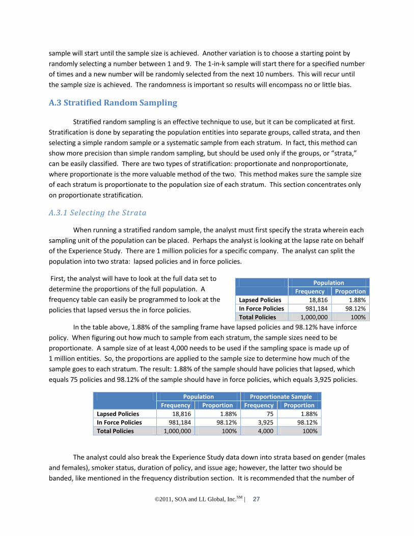
A.3.1 Selecting the Strata

When running a stratified random sample, the analyst must first specify the strata wherein each

sampling unit of the population can be placed. Perhaps the analyst is looking at the lapse rate on behalf

of the Experience Study. There are 1 million policies for a specific company. The analyst can split the

population into two strata: lapsed policies and in force policies.

First, the analyst will have to look at the full data set to

determine the proportions of the full population. A

frequency table can easily be programmed to look at the

policies that lapsed versus the in force policies.

In the table above, 1.88% of the sampling frame have lapsed policies and 98.12% have inforce

policy. When figuring out how much to sample from each stratum, the sample sizes need to be

proportionate. A sample size of at least 4,000 needs to be used if the sampling space is made up of

1 million entities. So, the proportions are applied to the sample size to determine how much of the

sample goes to each stratum. The result: 1.88% of the sample should have policies that lapsed, which

equals 75 policies and 98.12% of the sample should have in force policies, which equals 3,925 policies.

Population Proportionate Sample

Frequency Proportion Frequency Proportion

Lapsed Policies 18,816 1.88% 75 1.88%

In Force Policies 981,184 98.12% 3,925 98.12%

Total Policies 1,000,000 100% 4,000 100%

The analyst could also break the Experience Study data down into strata based on gender (males

and females), smoker status, duration of policy, and issue age; however, the latter two should be

banded, like mentioned in the frequency distribution section. It is recommended that the number of

Population

Frequency Proportion

Lapsed Policies 18,816 1.88%

In Force Policies 981,184 98.12%

Total Policies 1,000,000 100%


strata defined should not exceed five. Importantly, simple random sampling or systematic sampling

need to be performed on each stratum once the analyst calculates how many entities need to be pulled

for the sample.

A.3.2 Recommended Sample Sizes

Ho and Brancard tested out different sample sizes based on a certain

population size and recommend the following sample sizes in table E.

Compared to Simple Random Sampling, the sample sizes to the

associated sampling space, is significantly smaller using Stratification.

This supports the advantage that precision can be achieved at a smaller

cost. Note that the recommended sample sizes are meant to be used for

basic experience study analysis where only 2 stratification classes are

created. If additional fields are to be analyzed, it is recommended that

additional stratification classes are added. In these cases, minimum sample sizes would increase.

A.4 Random Cluster

Random cluster samplings are used when a population is too large or naturally has clusters, also

known as primary sampling units. This method differs from the other three because the groups are

those being randomly selected, not the individuals. Unfortunately, this sampling method doesn’t show

the most precision compared to simple random sampling and stratification, but it is still substantial,

especially when a budget exists. This method does show similarity to stratification, as both of them

have subgroups of the population; however, the cluster sampling method includes all of the entities in a

cluster (one-stage cluster), while the stratification method samples from each stratum.

This technique would be most appropriate to use if an analyst is looking at the number of life

insurance policies from certain companies. The analyst could perform a random cluster sample by

randomly selecting life insurance companies. For a one-stage cluster sample, the entities within these

companies would be part of the sample, also known as the primary sampling units. For a two-stage

cluster sample, the next step would be to randomly select a cluster of entities within the primary

sampling units. These clusters would then be considered secondary sampling units.

A.5 Recommendations for Sampling Techniques

There are many types of sampling techniques, although, Ho and Brancard believe that the four

mentioned sampling methods are the best choices for several reasons. Most importantly, these

methods produce samples that are representative of the populations. Additionally, at least one of these

methods is very attainable for a company’s own needs. As mentioned throughout the different sections,

advantages and disadvantages exist for each method. Table F was created to easily organize those

analyses.

Table E: Sample Size by Population

Population Sample Size

50,000,000 9,375

40,000,000 8,000

10,000,000 7,250

1,000,000 4,000

500,000 3,500

100,000 649


Table F: Advantages and Disadvantages of Sampling Methods

Method Advantage Disadvantage

Simple Random Sampling *Use if the population being used is fully up-to-date and time and money are not an issue.

Easy to create the sample.

Every entity of the population has an equal chance of being selected for the sample.

Unbiased

Representative of the population

The “list” must comprise the whole population being sampled. It may be hard to obtain the most current list.

It may be hard to go through a full list of entities, especially when the population is large.

This method could be very costly.

Need to use a certain sample size in order to obtain certain precision in results.

Systematic Sampling *Use if time and/or costs are limited. Although beware of hidden patterns when sample is collected.

Simple technique o May be less complicated to create

a program.

The population would be sampled uniformly.

The 1-in-k method could follow a certain pattern in the population. o This could ultimately leave the

sample biased and would not be representative of the population.

Stratified Random Sampling (Proportionate) *Use if proportions can be found from the main sampling frame and apply them to the sample. Also use if strata can be easily defined. Ho, Brancard prefer this method if the latter can be done.

More precision with a smaller sample size and less costs.

Very representative of the population.

Subgroups (strata) can be represented proportionately.

Strata can be hard to define.

Most complex method.

Cluster Sampling *Use when on a budget, when clusters naturally exist, or when clusters can easily be created.

Convenient to use when clusters naturally exist in the data.

Inexpensive

Simple technique

Data can be more complicated to analyze.

Larger sampling errors than other methods.

Least representative of the population compared with the other methods.

Entities within each cluster could be very similar and could lead to skewed results.


Data Quality Software Below is a list of popular data quality software current available on the market. This list does not

encompass all available software.

BDQS (BDQS)

Data Quality (Business Objects)

DataFlux (SAS)

Data State (IBM)

Data Quality (Informatica)

Trillium Software

Data Quality Tool (SOA)


Glossary Coding Errors – one of the Data Validity Errors. These are also called mapping or translation errors,

where the value of a field falls outside the acceptable values. For example, if the gender field

contains the values M, F, U, a value of X would be considered a coding error.

Data Accuracy Errors – second part of the data cleansing process. Data accuracy errors include

experience period, other missing values, and relational numeric field errors.

Data Cleansing – process of producing accurate and valid, error-free data.

Data Completeness Errors – part of the data validation process. Data completeness refers to the

amount of accurate and available data for use in the experience study analysis.

Data Consistency Errors – part of the data validation process. Data consistency checks for possible

errors through fluctuation of business across time.

Data Format Errors – one of the Data Validity Errors. These are errors with the wrong format.

Examples include inconsistent date fields (MM-DD-YY versus DD-MM-YY) as well numeric fields

showing up as characters (‘01’, ‘1 ‘, ‘ 1’).

Data Reasonability Errors – part of the data validation process. These errors are more easily seen

within the results of the experience study. Reasonability and trend of the results should exist.

Changes in trends, experience or spikes in lapse rates would signal potential data errors.

Data Validation – process of producing consistent, reasonable, and complete data.

Data Validity Errors– first part of the data cleansing process. Data validity errors include missing

values, coding errors, and format errors.

Experience Period Errors – one of the Data Accuracy Errors. This error is specific to data outside of

the experience period. Any policy not within the experience period is considered inaccurate. This

includes policies issued after the experience period and terminations not within the experience

period.

Inconsistency Errors – one of the Data Consistency Errors. Data used for experience studies, when

aggregate, should contain minimal fluctuation from study to study. This is especially true for

inter/intra-company studies and individual studies of companies with mature blocks of business.

Longitudinal Errors – one of the Data Consistency Errors. These errors occur when there are

changes to the inforce status of the policy between time spans of separate study. When these

studies are compiled into a larger experience study, longitudinal errors occur.

Missing Value Errors – one of the Data Validity Errors. These are errors within fields where values

are blank or zero but should not be.

Relationship of Numeric Field Errors – one of the Data Accuracy Errors. Certain numeric fields in

the experience data are relational to each other. Examples would be premium, face amount, and

cash value. Premium, or cash value, should never be greater than face amount.

Time Horizon Errors – one of the Data Consistency Errors. The time span of the experience data

should depend on the type of experience study and experience study results will be used. The

timing of the data as well as the time span of the data must be considered. Results from using older

experience data may not be reasonable and using one year’s worth of data may not be appropriate.


Bibliography

Actuarial References Actuarial IQ (Information Quality), CAS Data Management Educational Materials Working Party, 2009

ASOP No. 23: Data Quality, Actuarial Standards Board, 2004

Herzog, Thomas, Data Quality: Theory and Practice, SOA Annual Meeting, 2003

Herzog, Fritz, Williams, Data Quality and Record Linkage Techniques, New York: Spring Science + Business Media, 2007

Prevosto, Virginia R. , Is it time for your data’s annual check-up?, The Actuarial Digest, 2011

Spell, Darrell, Data Quality, SOA Health Valuation Bootcamp, 2009

Other Data Quality & Cleansing References Eckerson, Wayne W., Data Quality and the Bottom Line, The Data Warehouse Institute, 2001

McQuown, Gary , “SAS® Macros are the Cure for Quality Control Pains” <http://www2.sas.com/proceedings/sugi29/093-29.pdf>

Orli, Richard J., “Data Quality Methods” < http://www.kismeta.com/cleand1.html>,1996>

Tukey, Exploratory Data Analysis, New York: Addison Wesley, 1977

U.S. Social Security Administration, various publications.

Vannan, Elizabeth, Quality Data – An Improbable Dream?, Educause Quarterly, 2001

Statistics References “Determining Sample Size,” University of Florida IFAS Extension. <http://edis.ifas.ufl.edu/pd006> [Accessed 28 September 2011].

Hoel, Paul G., Elementary Statistics, 2nd ed., New York: London: Sydney: John Wiley and Sons, Inc., 1966.

“Organizational Research: Determining Appropriate Sample Size in Survey Research,” Organizational Systems Research Association. <http://www.osra.org/itlpj/bartlettkotrlikhiggins.pdf> [Accessed 28 September 2011].

Scheaffer, Richard L., Mendenhall III, William, and Ott, Lyman, Elementary Survey Sampling, 5th ed., Belmont: Duxbury Press, 1996.

“Simple Random Sampling,” Experiment-Resources. <http://www.experiment-resources.com/simple-random-sampling.html> [Accessed 28 September 2011].

Slonim, Morris James, Sampling: A Quick, Reliable Guide to Practical Statistics, New York: Simon and Schuster, 1960.

“Statistic, Probability, and Survey Sampling,” Stat Trek. <http://stattrek.com> [Accessed 28 September 2011].

http://www2.sas.com/proceedings/sugi29/093-29.pdf

http://www.kismeta.com/cleand1.html%3e,1996

http://edis.ifas.ufl.edu/pd006

http://www.osra.org/itlpj/bartlettkotrlikhiggins.pdf

http://www.experiment-resources.com/simple-random-sampling.html

http://www.experiment-resources.com/simple-random-sampling.html

http://stattrek.com/

009090-1211 (415-43-0-P28)

This publication is a benefit of LIMRA membership. No part may be shared with other organizations or reproduced in any form without the Society of Actuaries’ or LL Global’s written permission.

Documents

Experience Data Quality - Society of Actuaries