library/jacksonj

Help Booklet

Excel 2007

byJames Jackson

library/jacksonj

The Excel 2007 interface represents possibly the biggest change Microsoft has made to the look and feel of the program and to how you get at its myriad features. No matter what you do -- from opening files or adding formulas to creating charts or even just using a menu -- you’ll find things have changed.

1. The Microsoft Office button. The big button on the upper left-hand corner of the screen replaces the old File menu from previous versions of Excel. You’ll find familiar features for opening files, saving files, printing files and so on, but there’s a lot more here as well, as you’ll discover later in this guide.

2. The Quick Access Toolbar. Just to the right of the Office button is the Quick Access toolbar, with buttons for using Excel’s most common features, including Save, Undo, Redo, Sort, Print Preview and more, but you can add and remove buttons for any functions you please.

3. The Ribbon. Love it or hate it, the Ribbon is the main way you’ll work with Excel. Instead of old-style menus, in which menus have submenus, submenus have sub-submenus and so on, the Ribbon groups small icons for common tasks together in tabs on a big, well, ribbon. So, for example, when you click the Insert tab, the Ribbon appears with buttons for items that you can insert into a spreadsheet, such as charts, tables, pivot tables, clip art or a hyperlink.

4. The Scrollbar. This is largely unchanged from previous versions of Excel; use it to scroll up and down. There are a couple of minor changes. At the top, there’s a double arrow that when clicked upon, expands the area at the top of the worksheet that displays the contents of the current cell. Just below the double arrow is a tiny button that looks like a minus sign that lets you split your screen in two.

5. The View toolbar. There is now a View toolbar at the bottom right of the screen that lets you choose between Normal, Page Layout and Page Break Preview -- a view that will show you how your spreadsheet will look when it prints. There’s also a slider that lets you zoom in or out of your document.

The Toolbar

library/jacksonj

The Ribbon, by default, is divided into seven tabs, with an optional eighth one (Developer) that you can display by clicking the Office button and choosing Excel Options > Popular > Show Developer tab in the Ribbon.

Here’s a rundown of the tabs and what each one does:

Home: This contains commonly used Excel features, such as inserting formulas, formatting tables, rows, cells and text, and sorting and filtering.

Insert: As you might guess, this one handles anything you might want to insert into a document, such as charts, pivot tables, tables, pictures, clip art, text, WordArt.

Page layout: Here’s where you’ll change margins, page size and orientation, define your print area, set page breaks, specify which rows and columns will print on each page and so on.

Formulas: If you’re a spreadsheet jockey, you’ll be spending a lot of time on this tab. As the name says, it’s where you’ll go to insert and work with formulas. It organizes all of Excel’s formulas into categories, such as Financial, Logical, Math & Trig, and so on, so they’re all within easy reach. And it also gives you quick access to useful formula-checking features, such as error-checking and the ability to trace precedents and dependents.

Data: Whatever you need to do with data, you’ll find it here. For example, you can use this tab to import data from a wide variety of sources, including the Web, Access, SQL Server and so on. You’ll also be able to filter and sort data, validate your data, group and ungroup data, and perform data analysis, among other features.

Review: Need to check spelling and grammar, look up a word in a thesaurus, work in markup mode, review other people’s markups or compare documents? This is the tab for you. It also lets you protect worksheets and workbooks, and share workbooks.

View: Here’s where to go when you want to change the view in any way, including displaying or turning off gridlines and the formula bar, zooming in and out, splitting and hiding panes, and so on.

Developer: If you write code or create forms and applications for Excel, this is your tab. It also includes macro handling, so power users might also want to visit here every once in a while.

The Ribbon

library/jacksonj

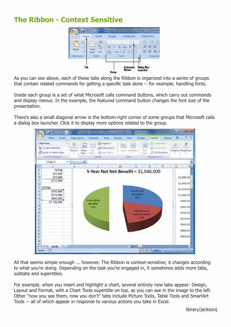
The Ribbon - Context Sensitive

All that seems simple enough ... however. The Ribbon is context-sensitive; it changes according to what you’re doing. Depending on the task you’re engaged in, it sometimes adds more tabs, subtabs and supertitles. For example, when you insert and highlight a chart, several entirely new tabs appear: Design, Layout and Format, with a Chart Tools supertitle on top, as you can see in the image to the left.Other “now you see them, now you don’t” tabs include Picture Tools, Table Tools and SmartArt Tools -- all of which appear in response to various actions you take in Excel.

As you can see above, each of these tabs along the Ribbon is organized into a series of groups that contain related commands for getting a specific task done -- for example, handling fonts.

Inside each group is a set of what Microsoft calls command buttons, which carry out commands and display menus. In the example, the featured command button changes the font size of the presentation.

There’s also a small diagonal arrow in the bottom-right corner of some groups that Microsoft calls a dialog box launcher. Click it to display more options related to the group.

library/jacksonj

The Office Button

There are two more new Excel tools that you’ll want to get to know -- the Office button and the Quick Access toolbar. Think of the Office button as a greatly expanded File menu from the Excel 2003 days -- the File menu on steroids. As you can see in the figure below, it’s where to go for the various Open, Save, New, Print and related options and also includes a list of all your recently opened files.

Clicking the Office button reveals everything the File menu used to, and more.

But there are three particularly noteworthy new features here as well -- Prepare, Publish and Convert. Convert lets you convert documents saved in older formats to the new Microsoft Office Open XML format, which is the new Office standard. For Excel, the extension is .xlsx. Publish does exactly what it says; it gives options for publishing a document. If your company uses a document management server or SharePoint, you can publish it there.

Use Prepare when you’ve finished your worksheet and are ready to share it with others. There are plenty of great options here, such as marking a document as final; encrypting the document; inspecting it for hidden metadata and information you’d prefer remain private; and adding a digital signature. Because Excel 2007 isn’t yet widely deployed, a particularly useful feature here is running the Compatibility Checker, which will let you know whether the worksheet contains features not supported by earlier Excel versions.

library/jacksonj

The Office Button - Customise

For those who like to fiddle with the Excel interface and how it works, the Excel Options button, located at the bottom of the Office button’s box, lets you customize Excel in many ways, including how you work with formulas, and rules for error-checking worksheets. It has many of the features that you accessed via Tools > Options in previous versions of Excel, plus more. It’s far better organized and easier to use than Tools > Options was.

Even those who can’t stand the Excel makeover and the Ribbon will find at least one thing to cheer about -- the Quick Access toolbar. This nifty little tool seems innocuous enough, but spend some time with it and you’ll see it’s one of the best additions to the new interface.The three buttons on the left -- Save, Undo and Redo -- aren’t particularly noteworthy, but the small icon to the right that looks like a small chart -- the Quick Layout button -- is exceedingly useful. Highlight a chart, click the button and a selection of premade chart layouts appear. Click the one you want, and it will immediately be applied to the chart.

Probably the most helpful customization for Excel 2007 is to add buttons the Quick Access toolbar, and there are several ways to do so. Directly to the right of the Quick Layout button, the nearly invisible Down arrow is the key to the Quick Access toolbar. Click it and you’ll be able to add and remove toolbar buttons for a preset list of about 10 commands.

To add buttons for additional commands, select More Commands from this list. The screen below appears. (You can also get to this screen by clicking the Office button and choosing Excel Options and then Customize.)

Adding buttons to the Quick Access toolbar.

Choose a command from the left-hand side of the screen that you want to add to the Quick Access toolbar and click Add. You can change the order of the buttons by highlighting a button on the right side of the screen and using the Up and Down arrows to move it.

The list of commands you see on the left may seem somewhat limited at first. That’s because Excel is showing you only the most popular commands. There are plenty of others you can add. Click the drop-down menu under “Choose commands from” at the top of the screen, and you’ll see other lists of commands -- All Commands, Home Tab and so on. Select any option, and there will be plenty of commands you can add.

library/jacksonj

Saving

On the Quick Access Toolbar, click Save, or press CTRL+S.

Type a name for the document, and then click Save.

Excel saves the document in a default location. To save the document in a different location, select another folder in the Favorite Links if your computer is running Windows Vista, or in the Save in list if your computer is running Microsoft Windows XP. If you want to change the default location where Excel saves documents, adjust the settings for saving documents.

Format

Excel Document (xlsx) - Excel 2007 format, can only be opened in Excel 2007

Excel 97-2003 Document (xls) - Standard format can be opened in Excel 2007 and all other versions of Excel. If you are not sure which version of Excel you have at home use this version.

library/jacksonj

If a file has been damaged and you cannot open it by normal means, you may be able to recover its content by using the Open and Repair feature.

Click the Microsoft Office Button , and then click Open.

Browse to the file that you want to recover, and click it (do not double-click it).

Click the arrow next to the Open button, and then click Open and Repair.

Open and Recover

Printing

Click the Microsoft Office Button , and then click Print.

Keyboard shortcut - To display the Print dialog box, press CTRL+P.

Click the options that you want, such as the number of slides or which slides you want to print.

Applies to programs that use the Microsoft Office Fluent user interface: To print without using the Print dialog box, click the Microsoft Office Button, point to the arrow next to Print, and then click Quick Print.

library/jacksonj

Keyboard Shortcuts

f you’re a fan of Excel 2003’s keyboard shortcuts, take heart -- most of them still work in 2007. So keep using them.

You can also use a clever set of keyboard shortcuts for working with the Ribbon. Press the Alt key and a tiny letter or number icon appears on the menu for each tab -- for example, the letter H for the Home tab. Now press that letter on your keyboard, and you’ll display that tab or menu item. When the tab appears, there will be letters and numbers for most options on the tab as well.

Using the Alt key helps you master the Ribbon.Once you’ve started to learn these shortcuts, you’ll naturally begin using key combinations. So instead of pressing Alt then H to display the home tab, you can press Alt-H together. The following table shows the most useful Alt key combinations in Excel 2007.

Excel 2007 Alt key combinations

Alt-F Office buttonAlt-H Home tabAlt-N Insert tabAlt-P Page Layout tabAlt-M Formulas tabAlt-A Data tabAlt-R Review tabAlt-W View tabAlt-L Developer tab

library/jacksonj

Sorting Data

Sorting data

Thishas been expanded to 64 levels. Best of all, while you can still sort data based on values (to sort a date column chronologically, for instance), you can also sort by font, color or icon used with conditional formatting. Thus, you can display all your green traffic lit cells together, followed by the yellow lights, then the red.

Other visualization tools eliminate the need for complicated macros or formulas. New conditional formatting options let you highlight duplicates, unique values, the top/bottom 10%, values above or below the average, cells less than or greater than a specified value, or cells within a range (highlighting cells containing values between 1 and 10, for example).

Pivot Tables

If you don’t need to see all values, the vastly improved Filter feature puts check boxes (for up to 1,000 values) in a pull-down list, allowing you to easily pick multiple values to display. Likewise, the new Remove Duplicates feature hides rows based on the duplicate values in columns you specify.

Among the notable improvements in Excel are tools to make existing features easier to use. Take PivotTables, for example. (For the uninitiated, PivotTables allow you to view your data differently -- think “slice and dice.” For example, you can summarize sales by agent by month or, with a simple drag-and-drop motion, summarize sales by month and within month by agent.)

In Excel 2007, you still set up PivotTables using a wizard, which is slightly changed from Excel 2003. However, once you have a PivotTable defined, manipulating it is considerably easier.

Instead of dragging and dropping elements within the table itself, you can use the wizard to make choices -- checking boxes to select which fields to display or choose sorting options, for example. Excel 2007 makes it easier to switch columns and rows, filter values, and use or hide field names. In addition, conditional formatting (those data bars or traffic lights we mentioned) can be applied to cells displayed in PivotTables.

library/jacksonj

Macros

At first glance, macros -- ingenious shortcuts you can create for performing repetitive tasks -- seem to have been banished from Excel 2007. But they’re still there; display the Developer tab, and you’ll find them in all their glory. In fact, the Developer toolbar puts the macro tools at easier reach than they were in previous versions of Excel.

All your macro controls are in the Code group on the Developer tab.You’ll find everything you want in the Code group on the Developer tab. Record a macro by click-ing the Record Macro button, manage your macros by clicking the Macros button and configure security for macros by clicking the Macro Security button.

Any macros you created in previous versions of Excel should work fine in Excel 2007.

Visualization Tools

Charts and graphs now support 16 million colors, and improved color support is evident through-out this version, especially in several new visual tools for highlighting data. For example, in Excel 2007 you can use conditional formatting to set the background color of a cell or use a colored bar (called a data bar) -- the length corresponds to the cell’s value.

You can also add icons to cells based on their value, giving your worksheet a dashboard-like qual-ity. For example, assigning traffic-light icons to a range of cells is a snap, and Excel’s built-in logic assigns colored circles based on the value of the cell: green for the highest third, yellow for the middle third and red for the bottom third.

Similarly, a four- or five-icon set (such as set of vertical bars similar to what your cell phone uses to indicate signal strength) displays icons based on which quartile or quintile the value falls into.

Conditional formatting rules are easy to adjust.In all cases, you can control the ranges for each icon in the set -- allowing you, for instance, to use a green traffic light to indicate only the highest 10% of values.

library/jacksonj

Themes

One of the promises of the Ribbon interface, according to Microsoft, is that some features are more obvious and usable. That’s certainly true of Styles, a formatting tool from previous versions of Excel that is now available using a “gallery” interface introduced in Office 2007.

You can quickly apply a collection of settings, from the font used to the background color and border style to cells, tables and PivotTables. As you mouse over the choices, Excel 2007 applies each style to your selection so you can preview the effect without making the change permanent.

One particularly noteworthy improvement to formatting is how Styles now respond to changes within your worksheet. In Excel 2003, you could apply a “green bar” effect so that the background color in rows alternated between green and white. However, once you added a row, the pattern was interrupted, and you needed to reapply the AutoFormat, a clumsy and awkward procedure.

In Excel 2007, that same pattern is adjusted whenever you add one or more rows. (Styles are equally smart when you add columns, for patterns that alternate between columns.) Styles will even adjust when you filter or hide rows or columns.

Themes, new to Office 2007, are style collections that include a color scheme, font, fill effects and more. Shared by several Office 2007 applications, themes can be applied to charts, tables and PivotTables in Excel, giving your work a consistent look and feel. That’s especially useful when you’re creating a chart that you want to copy to PowerPoint or Word.

To use Themes, select the Page Layout tab and click the Themes button to choose a new theme. You can also customize any theme or create new ones. One important caveat: Be aware that Themes only work if you’re using Word’s new Office XML format; they won’t work on old-style .xls files.

library/jacksonj

Table Tools

Excel’s new table features make it less likely you’ll have inconsistent formulas. Once you identify a contiguous range of cells as a table, Excel provides calculated columns. For example, if you add a column to the right of your table and enter a formula in any row, the formula will be copied to all cells in that new column, saving the time of executing a copy/paste command.

Even smarter, add a row and Excel is sure to include it in a total on the bottom row. (In previous versions of Excel, adding a row at the top or bottom of a range meant you risked omitting cells in that row from the sum formula.)

Furthermore, options on the Table Tools Design context-sensitive tab let you toggle the formatting of the first column or the first row. One click and you can add a Total row (though Excel lacks a similar command to add a Total column), then change what each column in that row computes (total, average, minimum and so on).

In addition, as you scroll down through a lengthy table, Excel replaces the column headings (the gray boxes with A/B/C above the columns) with values from the table’s header row -- a subtle improvement, to be sure, but it’s a more efficient technique than having to freeze rows to see column headings.

library/jacksonj

Format Changes

You’ll have to deal with four new XML-based file formats in Excel 2007 -- .xlsx for standard worksheets, .xlsm for those with macros, plus .xltx and .xltm for templates. Like Word 2007, Excel 2007 offers a compatibility checker and tells you if your workbook contains features that previous versions of Excel won’t support. Choose Office button > Prepare > Run Compatibility Checker to launch it.

If you’re sharing documents, you’ll probably want to save them in Excel 2003 format to maintain compatibility with other users -- at least until the new 2007 file format becomes the standard or you know your recipient has the free patch that lets Office 2003 users read and work with 2007 files.

Setting the default Save format.

To set Excel 2007 to save to the 2003 format by default, click on the Office button and then the Excel Options button. In the left panel of the screen that appears, click Save, then locate the “Save workbooks” area on the right. From the “Save files in this format” drop-down list, choose Excel 97-2003 Workbook and click OK.