HAL Id: hal-03241669https://hal.archives-ouvertes.fr/hal-03241669

Submitted on 28 May 2021

HAL is a multi-disciplinary open accessarchive for the deposit and dissemination of sci-entific research documents, whether they are pub-lished or not. The documents may come fromteaching and research institutions in France orabroad, or from public or private research centers.

L’archive ouverte pluridisciplinaire HAL, estdestinée au dépôt et à la diffusion de documentsscientifiques de niveau recherche, publiés ou non,émanant des établissements d’enseignement et derecherche français ou étrangers, des laboratoirespublics ou privés.

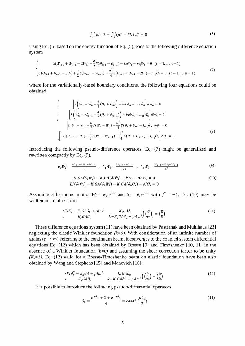
Exact Solutions for the Vibration of Finite GranularBeam Using Discrete and Gradient Elasticity Cosserat

ModelsSina Massoumi, Noël Challamel, Jean Lerbet

To cite this version:Sina Massoumi, Noël Challamel, Jean Lerbet. Exact Solutions for the Vibration of Finite GranularBeam Using Discrete and Gradient Elasticity Cosserat Models. Journal of Sound and Vibration,Elsevier, 2020. �hal-03241669�

1

Exact Solutions for the Vibration of Finite Granular Beam Using Discrete and Gradient Elasticity Cosserat Models

Sina Massoumi a, Noël Challamel b,*, Jean Lerbet a

a Univ. Evry – Université Paris-Saclay, Laboratoire de Mathématiques et Modélisation d’Evry, LaMME –UMR CNRS 8071, 23 bvd de France, 91037 Evry – France

b Univ. Bretagne Sud, IRDL – UBS – UMR CNRS 6027, Centre de Recherche, Rue de Saint Maudé – BP 92116, 56321 Lorient cedex – France

Abstract The present study theoretically investigates the free vibration problem of a discrete granular system. This problem can be considered as a simple model to rigorously study the effects of the microstructure on the dynamic behavior of the equivalent continuum structural model. The model consists of uniform grains confined by discrete elastic interactions, to take into account the lateral granular contributions. This repetitive discrete system can be referred to discrete Cosserat chain or a lattice elastic model with shear interaction. First for the simply supported granular beam resting on Winkler foundations, due to the critical frequencies which concern the nature of the dynamic results, the natural frequencies are exactly calculated, starting from the resolution of the linear difference eigenvalue problem. The natural frequencies of such a granular model are analytically calculated for whatever modes. It is shown that the difference equations governed to the discrete system converge to the differential equations of the Bresse-Timoshenko beam resting on Winkler foundation (also classified as a continuous Cosserat beam model) for an infinite number of grains. A gradient Bresse-Timoshenko model is constructed from continualization of the difference equations. This continuous gradient elasticity Cosserat model is obtained from a polynomial or a rational expansion of the pseudo-differential operators, stemming from the continualization process. Scale effects of the granular chain are captured by the continuous gradient elasticity model. The natural frequencies of the continuous gradient Cosserat models are compared with those of the discrete Cosserat model associated with the granular chain. The results clarify the dependency of the beam dynamic responses to the beam length ratio. Keywords: Granular medium; Cosserat continuum; Discrete Cosserat formulation; Gradient elasticity; Timoshenko beam.

* Corresponding author. E-mail address: noel.challamel@univ-ubs.fr.

2

1. Introduction In order to adapt a standard continuum theory to granular materials, it is necessary to

introduce the independent rotational degrees of freedom (DOF) in addition to the conventional translational ones. This helps to describe accurately the relative movements between the microstructure and the average macroscopic deformations. One may obtain higher-order gradient continua with additional degrees of freedom. One may also obtain Cosserat modeling that consequently leads to non-classical continuum or polar continuum theories (Cosserat type theories, e.g. Cosserat and Cosserat [1]; Nowacki [2]). Voigt [3] was the pioneer of developing this concept who first showed the existence of couple –stress in materials. Cosserat continuum theories belong to the larger class of generalized continua which introduce intrinsic length scales into continuum mechanics via higher-order gradients or additional degrees of freedom (Eringen [4, 5], Forest [6]). Feng [7] analyzed the behavior of the granular medium considering normal, shear and rotation interactions. In contrast, the classical continuum mechanics ignores the rotational interactions among particles and neglects the size effect of material particles. Schwartz et al. [8] studied dispersive analysis of a granular medium with normal and shear interactions neglecting the rotation effects.

On the other hand, in beam analysis, the Bresse-Timoshenko model takes into account both beam shear flexibility and rotatory inertia (Bresse [9] and Timoshenko [10, 11]). The effects of shear and rotational inertia can be significant in case of calculating eigenfrequencies for short beams, or in case of sufficiently small shear modulus. The Bresse-Timoshenko beam model is also a generalization of the Euler-Bernoulli model and admits a kinematics with two independent fields, a field of transverse displacement and a field of rotation. Timoshenko pointed out that the effects of cross-sectional dimensions on the beam dynamic behavior and frequencies could be significant. Timoshenko [10, 11] calculated the exact eigenfrequencies for such a beam with two degrees of freedom resting on two simple supports. Several lattice models have been developed based on microstructured Timoshenko in order to go further in understanding the structure behavior (see Ostoja-Starzewski [12] and Attar et al. [13]). The static and dynamic properties of a Cosserat-type lattice interface studied by Vasiliev et al. [14]. Calculation of eigenfrequencies for a Bresse-Timoshenko beam with any boundary conditions and elastic interaction with a rigid medium is obtained by Wang and Stephens [15], Manevich [16] or Elishakoff et al. [17] (see more recently Elishakoff [18] and Challamel and Elishakoff [19]). Bresse-Timoshenko beam theory is merely a one-dimensional Cosserat continuum medium by considering two independent translational and rotational degrees of freedom (Rubin [20] and Exadaktylos [21]). Thus, there is a fundamental link between these two continuum theories. In this paper, it is noticed the relation between Coasserat discrete theories and the continuum ones.

The present study focuses on the vibration of a granular beam with both bending and shear granular interactions. The granular beam is assumed to interact elastically with a rigid elastic support, a discrete elastic foundation labeled as a discrete Winkler foundation (Winkler [22]). Note that the difference equations governed to the model coincide with the ones of Cosserat granular model of Pasternak and Mühlhaus [23] in the absence of an elastic foundation, but differ from the ones of the discrete shear model studied by Duan et al. [24]. However, for some specific bending/ shear interaction modeling, the model developed by Bacigalupo and Gambarotta [25] can be mathematically reformulated with the difference equation presented in this paper.

This paper is arranged as follows: First, a discrete granular beam model is introduced from a geometrical and a mechanical point of view. The grain interaction and material parameters are defined in detail. Then from the dynamic analysis of the lattice beam model, the deflection

3

equations of the finite granular beam are derived. This fourth-order linear difference equation is solved by using the exact resolution of the difference equation. For an infinite number of grains, the deflection equation of a continuous beam (a fourth-order linear differential equation) is obtained asymptotically. Next, the eigenfrequencies of the discrete granular model and the continuous one, are obtained and compared as well. In the end, two asymptotic continualization methods are used to investigate continuous beam from the discrete lattice problem. With this aim, the polynomial expansion of Taylor and the rational expansion of Padé (with involved pseudo-differential operators) are used to derive new enriched beam models. These two nonlocal continualization approaches with the introduction of the gradient terms engage the neighbor influences which allow the passage from discrete result to continuous ones and simultaneously capture the length effect.

2. Granular Model A granular beam of length L resting on two simple supports is modeled by a finite number of grains interacting together. Such a model could be presented by considering the microstructured granular chain comprising n+1 rigid grains with diameter a (a=L/n) that are connected by n shear and rotational springs, as shown in Figure 1. It is assumed that the elastic support springs are located at the center of each rigid grain. Each grain has two degrees of freedom which are denoted by Wi for the deflection and 𝛩𝛩𝑖𝑖 for the rotation. This model is slightly different from the one of Challamel et al. [26] where the nodal kinematics and the Winkler elastic foundation are located at the grain interface. The aim of this paper consists in finding the vibration equation of this granular chain and then trying to obtain the natural frequencies.

(a)

(b)

4

Fig. 1. A discrete shear granular chain model composed of n+1 grain; (a) undeformed and (b) deformed.

The total kinetic energy of the model may be expressed as follows:

𝑇𝑇 =12�𝑚𝑚𝑖𝑖��𝑊𝑖𝑖

2𝑛𝑛

𝑖𝑖=0

+12�𝐼𝐼𝑚𝑚𝑖𝑖��𝛩𝑖𝑖

2𝑛𝑛

𝑖𝑖=0

(1)

where for i in [1, n-1], 𝐼𝐼𝑚𝑚𝑖𝑖 = 𝜌𝜌𝐼𝐼𝐼𝐼𝑛𝑛

= 𝜌𝜌𝐼𝐼𝐼𝐼 is the second moment of inertia of the beam segment and 𝑚𝑚𝑖𝑖 is the mass term for each grain that is defined for the inter grains by 𝑚𝑚𝑖𝑖 = 𝜌𝜌𝐼𝐼.

The strain energy function due to deformed shear spring (shear term) is given by

𝑈𝑈𝑠𝑠 =12�𝑆𝑆�𝑊𝑊𝑖𝑖+1 −𝑊𝑊𝑖𝑖 − 𝐼𝐼

𝛩𝛩𝑖𝑖+1 + 𝛩𝛩𝑖𝑖

2�2𝑛𝑛−1

𝑖𝑖=0

(2)

where S is the shear stiffness which can be expressed with respect to the shear stiffness 𝐾𝐾𝑠𝑠𝐺𝐺𝐺𝐺 of the equivalent beam. The shear stiffness parameter could be defined as 𝑆𝑆 = 𝐾𝐾𝑠𝑠𝐺𝐺𝐺𝐺

𝑎𝑎= 𝑛𝑛𝐾𝐾𝑠𝑠𝐺𝐺𝐺𝐺

𝐼𝐼 in

which G is the shear modulus, A is the cross-sectional area of the beam and Ks is an equivalent shear correction coefficient. In the present formulation, the kinematic variables are measured at nodes i located at the center of each grain, which is consistent with the approach followed for instance by Pasternak and Mühlhaus [23].

The strain energy function due to deformed rotational springs (bending term) may be obtained by

Ub =12� C(Θi+1 − Θi)2n−1

i=0

(3)

where C is the rotational stiffness located at the connection between each grain. This discrete stiffness can be expressed with respect to the bending stiffness EI of the equivalent beam and thus would be defined as 𝐶𝐶 = 𝐸𝐸𝐼𝐼

𝑎𝑎= 𝑛𝑛𝐸𝐸𝐼𝐼

𝐼𝐼 . where E is Young’s modulus and I is the second moment

of area. The elastic energy in the discrete elastic support (Winkler [22]) is given by

𝑈𝑈𝑊𝑊𝑖𝑖𝑛𝑛𝑊𝑊𝑊𝑊𝑊𝑊𝑊𝑊 =12�𝐾𝐾𝑊𝑊𝑖𝑖

2𝑛𝑛

𝑖𝑖=0

(4)

where K=ka is the discrete stiffness of the elastic support and is attached to the center of each grain.

The Lagrangian of the system may be defined as 𝐿𝐿 = 𝑇𝑇 − (𝑈𝑈𝑠𝑠 + 𝑈𝑈𝑏𝑏 + 𝑈𝑈𝑊𝑊𝑖𝑖𝑛𝑛𝑊𝑊𝑊𝑊𝑊𝑊𝑊𝑊) which slightly differs from the shear lattice model considered by Ostoja-Starzewski [12] for the shear term. By substituting the kinetic and potential terms, the Lagrangian may be expressed as:

𝐿𝐿 = �12∑ 𝑚𝑚𝑖𝑖��𝑊𝑖𝑖

2𝑛𝑛𝑖𝑖=0 + 1

2∑ 𝐼𝐼𝑚𝑚𝑖𝑖��𝛩𝑖𝑖

2𝑛𝑛𝑖𝑖=0 � − �1

2∑ 𝑆𝑆 �𝑊𝑊𝑖𝑖+1 −𝑊𝑊𝑖𝑖 − 𝐼𝐼 𝛩𝛩𝑖𝑖+1+𝛩𝛩𝑖𝑖

2�2

𝑛𝑛−1𝑖𝑖=0 + 1

2∑ 𝐶𝐶(𝛩𝛩𝑖𝑖+1 − 𝛩𝛩𝑖𝑖)2𝑛𝑛−1𝑖𝑖=0 +

12∑ 𝐾𝐾𝑊𝑊𝑖𝑖

2𝑛𝑛𝑖𝑖=0 �

(5)

The system of difference equations for both the discrete displacement and rotation fields is obtained from application of Hamilton’s principle, given by:

5

∫ 𝛿𝛿𝐿𝐿 𝑑𝑑𝑑𝑑𝑡𝑡2𝑡𝑡1

= ∫ (𝛿𝛿𝑇𝑇 − 𝛿𝛿𝑈𝑈) 𝑑𝑑𝑑𝑑𝑡𝑡2𝑡𝑡1

= 0 (6)

Using Eq. (6) based on the energy function of Eq. (5) leads to the following difference equation system

�𝑆𝑆(𝑊𝑊𝑖𝑖+1 + 𝑊𝑊𝑖𝑖−1 − 2𝑊𝑊𝑖𝑖) −

𝐼𝐼2 𝑆𝑆

(𝛩𝛩𝑖𝑖+1 − 𝛩𝛩𝑖𝑖−1) − 𝑘𝑘𝐼𝐼𝑊𝑊𝑖𝑖 − 𝑚𝑚𝑖𝑖��𝑊𝑖𝑖 = 0 (𝑖𝑖 = 1, … ,𝑛𝑛 − 1)

𝐶𝐶(𝛩𝛩𝑖𝑖+1 + 𝛩𝛩𝑖𝑖−1 − 2𝛩𝛩𝑖𝑖) +𝐼𝐼2 𝑆𝑆

(𝑊𝑊𝑖𝑖+1 −𝑊𝑊𝑖𝑖−1) −𝐼𝐼2

4 𝑆𝑆(𝛩𝛩𝑖𝑖+1 + 𝛩𝛩𝑖𝑖−1 + 2𝛩𝛩𝑖𝑖) − 𝐼𝐼𝑚𝑚𝑖𝑖��𝛩𝑖𝑖 = 0 (𝑖𝑖 = 1, … ,𝑛𝑛 − 1)

(7)

where for the variationally-based boundary conditions, the following four equations could be obtained

⎩⎪⎪⎪⎨

⎪⎪⎪⎧ �𝑆𝑆 �𝑊𝑊1 −𝑊𝑊0 −

𝐼𝐼2

(𝛩𝛩1 + 𝛩𝛩0)� − 𝑘𝑘𝐼𝐼𝑊𝑊0 − 𝑚𝑚0��𝑊0� 𝛿𝛿𝑊𝑊0 = 0

�𝑆𝑆 �𝑊𝑊𝑛𝑛 −𝑊𝑊𝑛𝑛−1 −𝐼𝐼2

(𝛩𝛩𝑛𝑛 + 𝛩𝛩𝑛𝑛−1)� + 𝑘𝑘𝐼𝐼𝑊𝑊𝑛𝑛 + 𝑚𝑚𝑛𝑛��𝑊𝑛𝑛� 𝛿𝛿𝑊𝑊𝑛𝑛 = 0

�𝐶𝐶(𝛩𝛩1 − 𝛩𝛩0) +𝐼𝐼2 𝑆𝑆

(𝑊𝑊1 −𝑊𝑊0) −𝐼𝐼2

4 𝑆𝑆(𝛩𝛩1 + 𝛩𝛩0) − 𝐼𝐼𝑚𝑚0��𝛩0� 𝛿𝛿𝛩𝛩0 = 0

�−𝐶𝐶(𝛩𝛩𝑛𝑛−1 − 𝛩𝛩𝑛𝑛) −𝐼𝐼2 𝑆𝑆

(𝑊𝑊𝑛𝑛 −𝑊𝑊𝑛𝑛−1) +𝐼𝐼2

4 𝑆𝑆(𝛩𝛩𝑛𝑛 + 𝛩𝛩𝑛𝑛−1) − 𝐼𝐼𝑚𝑚𝑛𝑛��𝛩𝑛𝑛� 𝛿𝛿𝛩𝛩𝑛𝑛 = 0

(8)

Introducing the following pseudo-difference operators, Eq. (7) might be generalized and rewritten compactly by Eq. (9).

𝛿𝛿0𝑊𝑊𝑖𝑖 = 𝑊𝑊𝑖𝑖+1+2𝑊𝑊𝑖𝑖+𝑊𝑊𝑖𝑖−14

, 𝛿𝛿1𝑊𝑊𝑖𝑖 = 𝑊𝑊𝑖𝑖+1−𝑊𝑊𝑖𝑖−12𝑎𝑎

, 𝛿𝛿2𝑊𝑊𝑖𝑖 = 𝑊𝑊𝑖𝑖+1−2𝑊𝑊𝑖𝑖+𝑊𝑊𝑖𝑖−1𝑎𝑎2

(9)

𝐾𝐾𝑠𝑠𝐺𝐺𝐺𝐺(𝛿𝛿2𝑊𝑊𝑖𝑖) − 𝐾𝐾𝑠𝑠𝐺𝐺𝐺𝐺(𝛿𝛿1𝛩𝛩𝑖𝑖) − 𝑘𝑘𝑊𝑊𝑖𝑖 − 𝜌𝜌𝐺𝐺��𝑊𝑖𝑖 = 0𝐸𝐸𝐼𝐼(𝛿𝛿2𝛩𝛩𝑖𝑖) + 𝐾𝐾𝑠𝑠𝐺𝐺𝐺𝐺(𝛿𝛿1𝑊𝑊𝑖𝑖) − 𝐾𝐾𝑠𝑠𝐺𝐺𝐺𝐺(𝛿𝛿0𝛩𝛩𝑖𝑖) − 𝜌𝜌𝐼𝐼𝛩𝛩𝚤𝚤

= 0

(10)

Assuming a harmonic motion 𝑊𝑊𝑖𝑖 = 𝑤𝑤𝑖𝑖𝑒𝑒𝑗𝑗𝑗𝑗𝑡𝑡 and 𝛩𝛩𝑖𝑖 = 𝜃𝜃𝑖𝑖𝑒𝑒𝑗𝑗𝑗𝑗𝑡𝑡 with 𝑗𝑗2 = −1, Eq. (10) may be written in a matrix form

�𝐸𝐸𝐼𝐼𝛿𝛿2 − 𝐾𝐾𝑠𝑠𝐺𝐺𝐺𝐺𝛿𝛿0 + 𝜌𝜌𝐼𝐼𝜔𝜔2 𝐾𝐾𝑠𝑠𝐺𝐺𝐺𝐺𝛿𝛿1𝐾𝐾𝑠𝑠𝐺𝐺𝐺𝐺𝛿𝛿1 𝑘𝑘−𝐾𝐾𝑠𝑠𝐺𝐺𝐺𝐺𝛿𝛿2 − 𝜌𝜌𝐺𝐺𝜔𝜔2� �

𝜃𝜃𝑤𝑤�𝑖𝑖

= �00� (11)

These difference equations system (11) have been obtained by Pasternak and Mühlhaus [23] neglecting the elastic Winkler foundation (k=0). With consideration of an infinite number of grains (𝑛𝑛 → ∞) referring to the continuum beam, it converges to the coupled system differential equations Eq. (12) which has been obtained by Bresse [9] and Timoshenko [10, 11] in the absence of a Winkler foundation (k=0) and assuming the shear correction factor to be unity (Ks=1). Eq. (12) valid for a Bresse-Timoshenko beam on elastic foundation have been also obtained by Wang and Stephens [15] and Manevich [16].

�𝐸𝐸𝐼𝐼𝜕𝜕𝑥𝑥2 − 𝐾𝐾𝑠𝑠𝐺𝐺𝐺𝐺 + 𝜌𝜌𝐼𝐼𝜔𝜔2 𝐾𝐾𝑠𝑠𝐺𝐺𝐺𝐺𝜕𝜕𝑥𝑥𝐾𝐾𝑠𝑠𝐺𝐺𝐺𝐺𝜕𝜕𝑥𝑥 𝑘𝑘−𝐾𝐾𝑠𝑠𝐺𝐺𝐺𝐺𝜕𝜕𝑥𝑥2 − 𝜌𝜌𝐺𝐺𝜔𝜔2� �

𝜃𝜃𝑤𝑤� = �0

0� (12)

It is possible to introduce the following pseudo-differential operators

𝛿𝛿0 =𝑒𝑒𝑎𝑎𝜕𝜕𝑥𝑥 + 2 + 𝑒𝑒−𝑎𝑎𝜕𝜕𝑥𝑥

4= 𝑐𝑐𝑐𝑐𝑐𝑐ℎ2 (

𝐼𝐼𝜕𝜕𝑥𝑥2

) (13)

6

𝛿𝛿1 =𝑒𝑒𝑎𝑎𝜕𝜕𝑥𝑥 − 𝑒𝑒−𝑎𝑎𝜕𝜕𝑥𝑥

2𝐼𝐼=𝑐𝑐𝑖𝑖𝑛𝑛ℎ (𝐼𝐼𝜕𝜕𝑥𝑥)

𝐼𝐼

𝛿𝛿2 =𝑒𝑒𝑎𝑎𝜕𝜕𝑥𝑥 − 2 + 𝑒𝑒−𝑎𝑎𝜕𝜕𝑥𝑥

𝐼𝐼2=

4𝐼𝐼2𝑐𝑐𝑖𝑖𝑛𝑛ℎ2 (

𝐼𝐼𝜕𝜕𝑥𝑥2

)

The relation could be obtained between these operators as

𝛿𝛿2𝛿𝛿0 = 𝛿𝛿0𝛿𝛿2 = 𝛿𝛿12 (14)

The same relations could be obtained for the pseudo-difference operators of Eq. (9). Going back to the discrete granular beam model Eq. (11), this characteristic equation has nontrivial solutions only if the determinant of the matrix is zero. Using the property of Eq. (14) gives the fourth-order difference equation for the deflection as follows:

[𝐸𝐸𝐼𝐼𝛿𝛿22 + �𝜌𝜌𝐼𝐼𝜔𝜔2 −

𝑘𝑘𝐸𝐸𝐼𝐼𝐾𝐾𝑠𝑠𝐺𝐺𝐺𝐺

+𝐸𝐸𝐼𝐼𝜌𝜌𝜔𝜔2

𝐾𝐾𝑠𝑠𝐺𝐺� 𝛿𝛿2 + (𝑘𝑘 − 𝜌𝜌𝐺𝐺𝜔𝜔2)𝛿𝛿0 −

𝑘𝑘𝜌𝜌𝐼𝐼𝜔𝜔2

𝐾𝐾𝑠𝑠𝐺𝐺𝐺𝐺+𝜌𝜌2𝐼𝐼𝜔𝜔4

𝐾𝐾𝑠𝑠𝐺𝐺]𝑤𝑤𝑖𝑖 = 0

(15)

[𝐸𝐸𝐼𝐼𝛿𝛿22 + �𝜌𝜌𝐼𝐼𝜔𝜔2 −

𝑘𝑘𝐸𝐸𝐼𝐼𝐾𝐾𝑠𝑠𝐺𝐺𝐺𝐺

+𝐸𝐸𝐼𝐼𝜌𝜌𝜔𝜔2

𝐾𝐾𝑠𝑠𝐺𝐺� 𝛿𝛿2 + (𝑘𝑘 − 𝜌𝜌𝐺𝐺𝜔𝜔2)𝛿𝛿0 −

𝑘𝑘𝜌𝜌𝐼𝐼𝜔𝜔2

𝐾𝐾𝑠𝑠𝐺𝐺𝐺𝐺+𝜌𝜌2𝐼𝐼𝜔𝜔4

𝐾𝐾𝑠𝑠𝐺𝐺]𝜃𝜃𝑖𝑖 = 0

(16)

Neglecting the Winkler elastic foundation (k=0), Eq. (15) leads to

[𝛿𝛿22 + 𝜔𝜔2 �

𝜌𝜌𝐸𝐸

+𝜌𝜌𝐾𝐾𝑠𝑠𝐺𝐺

�𝛿𝛿2 − 𝜔𝜔2(𝜌𝜌𝐺𝐺𝐸𝐸𝐼𝐼

𝛿𝛿0 −𝜌𝜌2𝜔𝜔2

𝐸𝐸𝐾𝐾𝑠𝑠𝐺𝐺)]𝑤𝑤𝑖𝑖 = 0

(17)

Duan et al. [24] also studied a discrete Timoshenko beam model based on rigid links where the displacement fields are defined at the joint element. The scheme of their study slightly differs from the granular model considered in this paper, essentially from the last term in the fourth-order difference equation of each model. The appearance of pseudo-difference operator δ0 in this model in comparison with Duan et al. [24], stems from the enhanced shear interaction modeling of the granular elements which refers to the fundamental difference of the two microstructural models.

[𝛿𝛿22 + 𝜔𝜔2 �

𝜌𝜌𝐸𝐸

+𝜌𝜌𝐾𝐾𝑠𝑠𝐺𝐺

�𝛿𝛿2 − 𝜔𝜔2(𝜌𝜌𝐺𝐺𝐸𝐸𝐼𝐼

−𝜌𝜌2𝜔𝜔2

𝐸𝐸𝐾𝐾𝑠𝑠𝐺𝐺)]𝑤𝑤𝑖𝑖 = 0

(18)

Eq. (17) and Eq. (18) are the governing deflection equations of two alternative discrete granular models for studying the beam vibration and its dynamic responses. The fourth-order difference equation Eq. (15) is equivalent to the one of Challamel et al. [27] in the static range (𝜔𝜔 = 0). Considering infinite number of grains (𝑛𝑛 → ∞) for the continuum beam, the fourth-order differential equation valid for a Bresse-Timoshenko beam on Winkler elastic foundation is given by Eq. (19) which also could be compared well by Wang and Stephens [15], Cheng and Pantelides [28] and Manevich [16].

𝑑𝑑4𝑤𝑤𝑑𝑑𝑥𝑥4

+ �𝜌𝜌𝑗𝑗2

𝐸𝐸�1 + 𝐸𝐸

𝑊𝑊𝑠𝑠𝐺𝐺� − 𝑊𝑊

𝑊𝑊𝑠𝑠𝐺𝐺𝐺𝐺� 𝑑𝑑

2𝑤𝑤𝑑𝑑𝑥𝑥2

− (𝜌𝜌𝑗𝑗2

𝐸𝐸�𝐺𝐺𝐼𝐼

+ 𝑊𝑊𝑊𝑊𝑠𝑠𝐺𝐺𝐺𝐺

− 𝜌𝜌𝑗𝑗2

𝑊𝑊𝑠𝑠𝐺𝐺� − 𝑊𝑊

𝐸𝐸𝐼𝐼)]𝑤𝑤 = 0 (19)

3. Exact Solution 3.1 Resolution of The Difference Equation In this section, the exact solution for the fourth-order linear difference eigenvalue problem

of Eq. (15) will be established (see the books of Goldberg [29] or Elaydi [30] for the general solution of linear difference equations). This approach, as detailed for instance by Elishakoff

7

and Santoro [31, 32], has been used to analyze the error in the finite difference based probabilistic dynamic problems. Eq. (15) and Eq. (16) restricted to the vibration terms, the linear fourth-order difference equation may be expanded as

(𝑤𝑤𝑖𝑖+2 − 4𝑤𝑤𝑖𝑖+1 + 6𝑤𝑤𝑖𝑖 − 4𝑤𝑤𝑖𝑖−1 + 𝑤𝑤𝑖𝑖−2) + 𝐼𝐼2 �𝜌𝜌𝐼𝐼𝐸𝐸𝐼𝐼𝜔𝜔2 − 𝑊𝑊

𝐾𝐾𝑠𝑠𝐺𝐺𝐺𝐺+ 𝜌𝜌𝐺𝐺𝑗𝑗2

𝐾𝐾𝑠𝑠𝐺𝐺𝐺𝐺� (𝑤𝑤𝑖𝑖+1 − 2𝑤𝑤𝑖𝑖 + 𝑤𝑤𝑖𝑖−1) +

𝐼𝐼4 � 𝑊𝑊4𝐸𝐸𝐼𝐼

− 𝜌𝜌𝐺𝐺𝑗𝑗2

4𝐸𝐸𝐼𝐼� (𝑤𝑤𝑖𝑖+1 + 2𝑤𝑤𝑖𝑖 + 𝑤𝑤𝑖𝑖−1) + 𝐼𝐼4(− 𝑊𝑊𝜌𝜌𝐼𝐼𝑗𝑗2

𝐸𝐸𝐼𝐼𝐾𝐾𝑠𝑠𝐺𝐺𝐺𝐺+ 𝜌𝜌2𝐼𝐼𝐺𝐺𝑗𝑗4

𝐸𝐸𝐼𝐼𝐾𝐾𝑠𝑠𝐺𝐺𝐺𝐺)𝑤𝑤𝑖𝑖 = 0

(20)

(𝜃𝜃𝑖𝑖+2 − 4𝜃𝜃𝑖𝑖+1 + 6𝜃𝜃𝑖𝑖 − 4𝜃𝜃𝑖𝑖−1 + 𝜃𝜃𝑖𝑖−2) + 𝐼𝐼2 �𝜌𝜌𝐼𝐼𝐸𝐸𝐼𝐼𝜔𝜔2 − 𝑊𝑊

𝐾𝐾𝑠𝑠𝐺𝐺𝐺𝐺+ 𝜌𝜌𝐺𝐺𝑗𝑗2

𝐾𝐾𝑠𝑠𝐺𝐺𝐺𝐺� (𝜃𝜃𝑖𝑖+1 − 2𝜃𝜃𝑖𝑖 + 𝜃𝜃𝑖𝑖−1) +

𝐼𝐼4 � 𝑊𝑊4𝐸𝐸𝐼𝐼

− 𝜌𝜌𝐺𝐺𝑗𝑗2

4𝐸𝐸𝐼𝐼� (𝜃𝜃𝑖𝑖+1 + 2𝜃𝜃𝑖𝑖 + 𝜃𝜃𝑖𝑖−1) + 𝐼𝐼4(− 𝑊𝑊𝜌𝜌𝐼𝐼𝑗𝑗2

𝐸𝐸𝐼𝐼𝐾𝐾𝑠𝑠𝐺𝐺𝐺𝐺+ 𝜌𝜌2𝐼𝐼𝐺𝐺𝑗𝑗4

𝐸𝐸𝐼𝐼𝐾𝐾𝑠𝑠𝐺𝐺𝐺𝐺)𝜃𝜃𝑖𝑖 = 0

(21)

As was mentioned in the previous section these two equation systems are true for all grains except the two ends. For simply supported boundary conditions as shown in figure 1 and with respect to Eq. (8), the four boundary conditions are formulated as:

⎩⎪⎨

⎪⎧

𝑊𝑊0 = 0𝑊𝑊𝑛𝑛 = 0

𝐶𝐶(𝛩𝛩1 − 𝛩𝛩0) + 𝑎𝑎2𝑆𝑆(𝑊𝑊1 −𝑊𝑊0) − 𝑎𝑎2

4𝑆𝑆(𝛩𝛩1 + 𝛩𝛩0) − 𝐼𝐼𝑚𝑚0��𝛩0 = 0

𝐶𝐶(𝛩𝛩𝑛𝑛 − 𝛩𝛩𝑛𝑛−1) + 𝑎𝑎2𝑆𝑆(𝑊𝑊𝑛𝑛 −𝑊𝑊𝑛𝑛−1) − 𝑎𝑎2

4𝑆𝑆(𝛩𝛩𝑛𝑛 + 𝛩𝛩𝑛𝑛−1) + 𝐼𝐼𝑚𝑚𝑛𝑛��𝛩𝑛𝑛 = 0

(22)

The two last equations of Eq. (22) are actually second-newton laws for the boundary grains and could be rewritten in the compact form by

𝑀𝑀1/2 + 𝑎𝑎

2𝑉𝑉1/2 = 𝐼𝐼𝑚𝑚0��𝛩0

−𝑀𝑀𝑛𝑛−1/2 −𝑎𝑎2𝑉𝑉𝑛𝑛−1/2 = 𝐼𝐼𝑚𝑚𝑛𝑛��𝛩𝑛𝑛

(23)

where

𝑀𝑀1/2 = 𝐶𝐶(𝛩𝛩1 − 𝛩𝛩0), 𝑉𝑉1/2 =𝐼𝐼2𝑆𝑆 �𝑊𝑊1 −𝑊𝑊0 −

𝐼𝐼2

(𝛩𝛩1 + 𝛩𝛩0)�

𝑀𝑀𝑛𝑛−1/2 = 𝐶𝐶(𝛩𝛩𝑛𝑛 − 𝛩𝛩𝑛𝑛−1), 𝑉𝑉𝑛𝑛−1/2 =𝐼𝐼2𝑆𝑆(𝑊𝑊𝑛𝑛 −𝑊𝑊𝑛𝑛−1 −

𝐼𝐼2

(𝛩𝛩𝑛𝑛 + 𝛩𝛩𝑛𝑛−1))

(24)

On the other hand, Eq. (7) could be applied for the boundary grains by considering two fictitious grains (i=-1 and i=n+1) connected to the system with fictitious springs. The equilibrium conditions of the boundary grains could be written by Eq. (25).

𝑀𝑀1/2 − 𝑀𝑀−1/2 +𝐼𝐼2

(𝑉𝑉1/2 − 𝑉𝑉−1/2) = 𝐼𝐼𝑚𝑚0��𝛩0

𝑀𝑀𝑛𝑛−1/2 − 𝑀𝑀𝑛𝑛+1/2 +𝐼𝐼2

(𝑉𝑉𝑛𝑛−1/2 − 𝑉𝑉𝑛𝑛+1/2) = 𝐼𝐼𝑚𝑚𝑛𝑛��𝛩𝑛𝑛

(25)

where

𝑀𝑀−1/2 = 𝐶𝐶(𝛩𝛩0 − 𝛩𝛩−1), 𝑉𝑉−1/2 =𝐼𝐼2𝑆𝑆(𝑊𝑊0 −𝑊𝑊−1 −

𝐼𝐼2

(𝛩𝛩0 + 𝛩𝛩−1))

𝑀𝑀𝑛𝑛+1/2 = 𝐶𝐶(𝛩𝛩𝑛𝑛+1 − 𝛩𝛩𝑛𝑛), 𝑉𝑉𝑛𝑛+1/2 =𝐼𝐼2𝑆𝑆(𝑊𝑊𝑛𝑛+1 −𝑊𝑊𝑛𝑛 −

𝐼𝐼2

(𝛩𝛩𝑛𝑛+1 + 𝛩𝛩0))

(26)

The antisymmetric conditions lead to:

8

𝑀𝑀−1/2 = −𝑀𝑀1/2, 𝑉𝑉−1/2 = 𝑉𝑉1/2

𝑀𝑀𝑛𝑛+1/2 = −𝑀𝑀𝑛𝑛−1/2, 𝑉𝑉𝑛𝑛+1/2 = 𝑉𝑉𝑛𝑛−1/2

(27)

Ones could be concluded that

𝛩𝛩1 = 𝛩𝛩−1 , 𝑊𝑊1 = −𝑊𝑊−1

𝛩𝛩𝑛𝑛−1 = 𝛩𝛩𝑛𝑛+1, 𝑊𝑊𝑛𝑛−1 = −𝑊𝑊𝑛𝑛+1

(28)

Using the recent conditions in Eq. (7) for i=0 and i=n, leads to

𝐶𝐶(𝛩𝛩1 − 𝛩𝛩0) +

𝐼𝐼2𝑆𝑆(𝑊𝑊1 −𝑊𝑊−1 −

𝐼𝐼2

(𝛩𝛩1 + 𝛩𝛩0)) −𝐼𝐼𝑚𝑚0

2��𝛩0 = 0

𝐶𝐶(𝛩𝛩𝑛𝑛−1 − 𝛩𝛩𝑛𝑛) +𝐼𝐼2𝑆𝑆(𝑊𝑊𝑛𝑛+1 −𝑊𝑊𝑛𝑛−1 −

𝐼𝐼2

(𝛩𝛩𝑛𝑛 + 𝛩𝛩𝑛𝑛−1)) −𝐼𝐼𝑚𝑚𝑛𝑛

2��𝛩𝑛𝑛 = 0

(29)

where 𝐼𝐼𝑚𝑚0 and 𝐼𝐼𝑚𝑚𝑛𝑛 represent the second moment of inertia for the boundary grains with consideration of the fictitious elements (i=-1 and n+1). Comparing the two systems of equations Eq. (22) and Eq. (29) result that the fictitious system behaves the same as the real model with the associated boundary conditions as follows:

𝐺𝐺𝑑𝑑 𝑖𝑖 = 0 ∶ 𝑤𝑤0 = 0 ; 𝑤𝑤1 = −𝑤𝑤−1 → 𝛿𝛿2𝑤𝑤0 = 0

𝐺𝐺𝑑𝑑 𝑖𝑖 = 𝑛𝑛 ∶ 𝑤𝑤𝑛𝑛 = 0 ; 𝑤𝑤𝑛𝑛−1 = −𝑤𝑤𝑛𝑛+1 → 𝛿𝛿2𝑤𝑤𝑛𝑛 = 0

(30)

These boundary conditions have been used also by Hunt et al. [33] for the problem of static bifurcation of granular chains under axial load. The non-dimensional quantities may be introduced

𝛺𝛺2 = 𝑗𝑗2𝜌𝜌𝐺𝐺𝐼𝐼4

𝐸𝐸𝐼𝐼 , 𝜇𝜇𝑠𝑠 = 𝐸𝐸

𝐾𝐾𝑠𝑠 𝐺𝐺 , 𝑟𝑟 = �𝐼𝐼

𝐺𝐺 , 𝑟𝑟∗ = 𝑊𝑊

𝐼𝐼 , 𝑘𝑘∗ = 𝑊𝑊𝐼𝐼4

𝐸𝐸𝐼𝐼

(31)

𝛺𝛺 is a dimensionless frequency; 𝜇𝜇𝑠𝑠 is inversely proportional to the shear stiffness; and 𝑟𝑟∗ is proportional to the rotatory inertia. The solution of the linear difference equation is thought in the form

𝑤𝑤𝑖𝑖 = 𝐵𝐵𝜆𝜆𝑖𝑖 (32)

where B is a constant. Therefore the characteristic equation could be obtained by replacing Eq. (32) in Eq. (20) as

(𝜆𝜆 +1𝜆𝜆

)2 + �𝜆𝜆 +1𝜆𝜆� 𝜖𝜖 + 𝜏𝜏 = 0 (33)

where the parameters 𝜖𝜖 and 𝜏𝜏 can be defined as

𝜖𝜖 = �𝑟𝑟∗2𝛺𝛺2

𝑛𝑛2�1 + 𝜇𝜇𝑠𝑠 −

14𝑟𝑟∗2𝑛𝑛2

� −𝑟𝑟∗2𝑘𝑘∗𝜇𝜇𝑠𝑠𝑛𝑛2

+𝑘𝑘∗

4𝑛𝑛4− 4�,

𝜏𝜏 = �𝑟𝑟∗2𝛺𝛺2

𝑛𝑛4�−𝜇𝜇𝑠𝑠𝑟𝑟∗

2𝑘𝑘∗ + 𝜇𝜇𝑠𝑠𝑟𝑟∗2𝛺𝛺2� + 2�

𝑘𝑘∗

4𝑛𝑛4−𝛺𝛺2

4𝑛𝑛4� − 2(

𝑟𝑟∗2𝛺𝛺2

𝑛𝑛2(1 + 𝜇𝜇𝑠𝑠) −

𝑟𝑟∗2𝑘𝑘∗𝜇𝜇𝑠𝑠𝑛𝑛2

) + 4�

(34)

Solving Eq. (33) leads to the equation obtained by Zhang et al. [34] which could be written

9

𝜆𝜆 +1𝜆𝜆

=−𝜖𝜖 ± √𝜖𝜖2 − 4 𝜏𝜏

2

(35)

Eq. (35) admits four solutions written

𝜆𝜆1,2 =−𝜖𝜖 + √𝜖𝜖2 − 4 𝜏𝜏

4± �(

𝜖𝜖 − √𝜖𝜖2 − 4 𝜏𝜏4

)2 − 1 (36)

𝜆𝜆3,4 =−𝜖𝜖 − √𝜖𝜖2 − 4 𝜏𝜏

4± 𝑗𝑗�1 − (

𝜖𝜖 + √𝜖𝜖2 − 4 𝜏𝜏4

)2 (37)

where 𝑗𝑗2 = −1. On the other hand, it is important to notice that according to Eq. (35) the results of 𝜆𝜆 + 1

𝜆𝜆 are in the ranges of (−∞, −2] or [2, +∞).

The limited cases when 𝜆𝜆 + 1𝜆𝜆 = ±2 would happen for 𝜆𝜆 = ±1 which refers to the critical

frequencies. The critical frequencies of the system are inconsistent condition with Eq. (32) would be obtained by assuming:

𝜏𝜏 = ±2𝜖𝜖 − 4 (38)

Replacing 𝜏𝜏 and 𝜖𝜖 by using Eq. (34), ones could be obtained as:

(𝑟𝑟∗2𝛺𝛺𝑐𝑐𝑊𝑊2

𝑛𝑛2− 4)(

𝜇𝜇𝑠𝑠𝑟𝑟∗2

𝑛𝑛2(𝛺𝛺𝑐𝑐𝑊𝑊2 − 𝑘𝑘∗) − 4) = 0

(39)

1𝑛𝑛4

((𝛺𝛺𝑐𝑐𝑊𝑊2 − 𝑘𝑘∗)(𝜇𝜇𝑠𝑠 𝑟𝑟∗4𝛺𝛺𝑐𝑐𝑊𝑊2 − 1)) = 0 (40)

Therefore, two branches of critical frequencies would be obtained as follows

𝛺𝛺𝑐𝑐𝑊𝑊1,1 = 2𝑛𝑛𝑟𝑟∗

, 𝛺𝛺𝑐𝑐𝑊𝑊1,2 = �4𝑛𝑛2

𝜇𝜇𝑠𝑠𝑟𝑟∗2+ 𝑘𝑘∗

(41)

𝛺𝛺𝑐𝑐𝑊𝑊2,1 = √𝑘𝑘∗ , 𝛺𝛺𝑐𝑐𝑊𝑊2,2 = �1

𝜇𝜇𝑠𝑠𝑟𝑟∗4

(42)

The critical frequencies of the first branch depend on the grain number (microstructure parameter), mechanical properties and beam geometry (macrostructure parameters) while the second branch critical frequencies are only defined as a function of the beam mechanical properties and geometry. On the other hand, comparing these critical values with the those of the Timoshenko continuum beam resting on the Winkler foundations (see Wang and Stephens [15]), leads to the equivalency of the second branch critical values (Eq. (42)) to the Timoshenko continuum beam’s. For an infinite number of grains, since the first branch critical frequencies (𝛺𝛺𝑐𝑐𝑊𝑊1,1 and 𝛺𝛺𝑐𝑐𝑊𝑊1,2) leads to infinite values and consequently disappear, so only the second branch would remain. These critical values could be shown as follows

𝜔𝜔𝑐𝑐𝑊𝑊2,1 = 𝜔𝜔𝑐𝑐𝑊𝑊𝑇𝑇𝑖𝑖𝑇𝑇𝑇𝑇𝑠𝑠ℎ𝑒𝑒𝑛𝑛𝑒𝑒𝑇𝑇 1 = �𝑘𝑘𝜌𝜌𝐺𝐺

, 𝜔𝜔𝑐𝑐𝑊𝑊2,2 = 𝜔𝜔𝑐𝑐𝑊𝑊𝑇𝑇𝑖𝑖𝑇𝑇𝑇𝑇𝑠𝑠ℎ𝑒𝑒𝑛𝑛𝑒𝑒𝑇𝑇 2 = �𝐾𝐾𝑠𝑠 𝐺𝐺𝐺𝐺𝜌𝜌𝐼𝐼

(43)

10

The behavior of the beam deflection solution would be separated by the critical frequencies into different regimes and depending on the frequencies values, the results would be in a distinct manner. For a finite number of grains, four regimes would be occurred categorized as follows: when 0 < 𝛺𝛺 < 𝛺𝛺𝑐𝑐𝑊𝑊2,2 there are two exponential terms and two traveling waves since 𝜆𝜆1,2 are real and 𝜆𝜆3,4 are imaginary. In this case, the deflection equation form would be obtained from Eq. (54).

When 𝛺𝛺𝑐𝑐𝑊𝑊2,2 < 𝛺𝛺 < 𝛺𝛺𝑐𝑐𝑊𝑊1,2 , 𝜆𝜆1,2,3,4 are all imaginary and therefore all terms represent traveling waves and for this case the deflection equation form would be obtained from Eq. (55). For 𝛺𝛺𝑐𝑐𝑊𝑊1,2 < 𝛺𝛺 < 𝛺𝛺𝑐𝑐𝑊𝑊1,1 again there are two exponential terms and two traveling waves since 𝜆𝜆1,2 are imaginary and 𝜆𝜆3,4 are real and the deflection equation form would be obtained from Eq. (56). Finally, for 𝛺𝛺𝑐𝑐𝑊𝑊1,1 < 𝛺𝛺 , since all parameters of 𝜆𝜆1,2,3,4 are real, thus whole terms represent exponential terms which leads to the deflection equation form of Eq. (57).

For specific value of grain number 𝛺𝛺𝑐𝑐𝑊𝑊1,1 and 𝛺𝛺𝑐𝑐𝑊𝑊2,2 would be equal together. This leads to the reduction of the four regimes to three.

𝑛𝑛 = 1

2𝑟𝑟∗�𝜇𝜇𝑠𝑠 =

𝐿𝐿2�𝐾𝐾𝑠𝑠 𝐺𝐺𝐺𝐺

𝐸𝐸𝐼𝐼

(44)

The results are shown for a case study of 50 grains and the dimensionless parameters of 𝜇𝜇𝑠𝑠 =4.28, 𝑟𝑟∗ = 0.029, 𝑘𝑘∗ = 15 in Figure 2. In this example, the values of the critical frequencies are respectively 𝛺𝛺𝑐𝑐𝑊𝑊1,1 = 3464.1, 𝛺𝛺𝑐𝑐𝑊𝑊1,2 = 1673.7, 𝛺𝛺𝑐𝑐𝑊𝑊2,1 = 3.87 and 𝛺𝛺𝑐𝑐𝑊𝑊2,2 = 579.8.

(a) (b)

(c) (d)

(e) (f)

(g) (h)

11

Fig. 2. Schematic behavior of the wave vector regarding the eigenfrequencies for finite grain number (n=50). (a), (c), (e) and (g) correspond to the real part and (b), (d), (f) and (h) correspond to the imaginary part of the wave vector.

For an infinite number of grains, since the first two critical values converge to the infinite, so the previous different regimes reduce to two regimes: when 0 < 𝛺𝛺 < 𝛺𝛺𝑐𝑐𝑊𝑊2,2 there are two exponential terms and two traveling waves as 𝜆𝜆1,2 are real and 𝜆𝜆3,4 are imaginary and thus the deflection equation form would be obtained from Eq. (54). When 𝛺𝛺𝑐𝑐𝑊𝑊2,2 < 𝛺𝛺 , 𝜆𝜆1,2,3,4 are all imaginary and thus all terms represent traveling waves. This case leads to the deflection equation form of Eq. (55). These two regimes correspond to the ones obtained for the continuum beam of Timoshenko resting on Winkler foundations.

(a) (b)

(c) (d)

(e) (f)

(g) (h)

Fig. 3. The effects of the eigenfrequencies on the wave behavior for a general discrete beam contains infinite grain number (𝑛𝑛 → ∞). (a), (c), (e) and (g) correspond to the real part and (b), (d), (f) and (h) correspond to the imaginary part of the wave vector.

Therefore, 𝜆𝜆1,2 can be rewritten for 𝛺𝛺 < 𝛺𝛺𝑐𝑐𝑊𝑊2,2 and 𝛺𝛺𝑐𝑐𝑊𝑊1,2 < 𝛺𝛺 (see also Elishakoff and Santoro [32] for a similar presentation applied to the finite difference formulation of Euler-Bernoulli beams) as

12

𝜆𝜆1,2 = 𝑐𝑐𝑐𝑐𝑐𝑐ℎ 𝜗𝜗 ± 𝑐𝑐𝑖𝑖𝑛𝑛ℎ 𝜗𝜗 (45)

where

𝑐𝑐𝑐𝑐𝑐𝑐ℎ 𝜗𝜗 =−𝜖𝜖4

+12��

−𝜖𝜖2

�2− 𝜏𝜏 =

−𝜖𝜖2− 𝑐𝑐𝑐𝑐𝑐𝑐𝑐𝑐

(46)

𝑐𝑐𝑐𝑐𝑐𝑐 𝑐𝑐 =−𝜖𝜖4−

12��

−𝜖𝜖2

�2− 𝜏𝜏

(47)

while 𝜆𝜆1,2 would be obtained for 𝛺𝛺𝑐𝑐𝑊𝑊2,2 < 𝛺𝛺 < 𝛺𝛺𝑐𝑐𝑊𝑊1,2

𝜆𝜆1,2 = 𝑐𝑐𝑐𝑐𝑐𝑐𝜗𝜗 ± 𝑗𝑗𝑐𝑐𝑖𝑖𝑛𝑛𝜗𝜗 (48)

where

𝑐𝑐𝑐𝑐𝑐𝑐 𝜗𝜗 =−𝜖𝜖4

+12��

−𝜖𝜖2

�2− 𝜏𝜏

(49)

On the other hand, 𝜆𝜆3,4 would be defined for 𝛺𝛺 < 𝛺𝛺𝑐𝑐𝑊𝑊1,1 by

𝜆𝜆3,4 = 𝑐𝑐𝑐𝑐𝑐𝑐𝑐𝑐 ± 𝑗𝑗𝑐𝑐𝑖𝑖𝑛𝑛𝑐𝑐 (50)

where

𝑐𝑐 = 𝐼𝐼𝑟𝑟𝑐𝑐𝑐𝑐𝑐𝑐𝑐𝑐 (−𝜖𝜖4− 1

2��−𝜖𝜖

2 �2− 𝜏𝜏)

(51)

And for 𝛺𝛺𝑐𝑐𝑊𝑊1,1 < 𝛺𝛺

𝜆𝜆3,4 = 𝑐𝑐𝑐𝑐𝑐𝑐ℎ𝑐𝑐 ± 𝑐𝑐𝑖𝑖𝑛𝑛ℎ𝑐𝑐 (52)

𝑐𝑐 = 𝐼𝐼𝑟𝑟𝑐𝑐𝑐𝑐𝑐𝑐𝑐𝑐ℎ (−𝜖𝜖4− 1

2��−𝜖𝜖

2 �2− 𝜏𝜏)

(53)

In view of Eq. (46) and (47), there are three possible general solutions for 𝑤𝑤𝑖𝑖 depending on the critical values of the frequencies which may be represented as

𝑤𝑤𝑖𝑖 = 𝐺𝐺1 𝑐𝑐𝑐𝑐𝑐𝑐 𝑖𝑖𝑐𝑐 + 𝐺𝐺2 𝑐𝑐𝑖𝑖𝑛𝑛 𝑖𝑖𝑐𝑐 + 𝐺𝐺3 𝑐𝑐𝑐𝑐𝑐𝑐ℎ 𝑖𝑖𝜗𝜗 + 𝐺𝐺4 𝑐𝑐𝑖𝑖𝑛𝑛ℎ 𝑖𝑖𝜗𝜗 (𝛺𝛺 < 𝛺𝛺𝑐𝑐𝑊𝑊2,2 ) (54)

𝑤𝑤𝑖𝑖 = 𝐵𝐵1 𝑐𝑐𝑐𝑐𝑐𝑐 𝑖𝑖𝑐𝑐 + 𝐵𝐵2 𝑐𝑐𝑖𝑖𝑛𝑛 𝑖𝑖𝑐𝑐 + 𝐵𝐵3 𝑐𝑐𝑐𝑐𝑐𝑐 𝑖𝑖𝜗𝜗 + 𝐵𝐵4 𝑐𝑐𝑖𝑖𝑛𝑛 𝑖𝑖𝜗𝜗 (𝛺𝛺𝑐𝑐𝑊𝑊2,2 < 𝛺𝛺 < 𝛺𝛺𝑐𝑐𝑊𝑊1,2 ) (55)

𝑤𝑤𝑖𝑖 = 𝐶𝐶1 𝑐𝑐𝑐𝑐𝑐𝑐ℎ 𝑖𝑖𝑐𝑐 + 𝐶𝐶2 𝑐𝑐𝑖𝑖𝑛𝑛ℎ 𝑖𝑖𝑐𝑐 + 𝐶𝐶3 𝑐𝑐𝑐𝑐𝑐𝑐 𝑖𝑖𝜗𝜗 + 𝐶𝐶4 𝑐𝑐𝑖𝑖𝑛𝑛 𝑖𝑖𝜗𝜗 (𝛺𝛺𝑐𝑐𝑊𝑊1,2 < 𝛺𝛺 < 𝛺𝛺𝑐𝑐𝑊𝑊1,1 ) (56)

𝑤𝑤𝑖𝑖 = 𝐷𝐷1 𝑐𝑐𝑐𝑐𝑐𝑐ℎ 𝑖𝑖𝑐𝑐 + 𝐷𝐷2 𝑐𝑐𝑖𝑖𝑛𝑛ℎ 𝑖𝑖𝑐𝑐 + 𝐷𝐷3 𝑐𝑐𝑐𝑐𝑐𝑐ℎ 𝑖𝑖𝜗𝜗 + 𝐷𝐷4 𝑐𝑐𝑖𝑖𝑛𝑛ℎ 𝑖𝑖𝜗𝜗 (𝛺𝛺𝑐𝑐𝑊𝑊1,1 < 𝛺𝛺 ) (57)

For the simply supported discrete system by substituting Eq. (30) in Eq. (54), (55), (56) and (57) the boundary conditions could be defined in matrix form, respectively

13

�

1𝑐𝑐𝑐𝑐𝑐𝑐(𝑛𝑛𝑐𝑐)2 𝑐𝑐𝑐𝑐𝑐𝑐 𝑐𝑐

2𝑐𝑐𝑐𝑐𝑐𝑐 𝑐𝑐 𝑐𝑐𝑐𝑐𝑐𝑐(𝑛𝑛𝑐𝑐)

0𝑐𝑐𝑖𝑖𝑛𝑛(𝑛𝑛𝑐𝑐)

02𝑐𝑐𝑐𝑐𝑐𝑐 𝑐𝑐 𝑐𝑐𝑖𝑖𝑛𝑛(𝑛𝑛𝑐𝑐)

1𝑐𝑐𝑐𝑐𝑐𝑐ℎ(𝑛𝑛𝜗𝜗)2 𝑐𝑐𝑐𝑐𝑐𝑐ℎ 𝜗𝜗

2 𝑐𝑐𝑐𝑐𝑐𝑐ℎ 𝜗𝜗 𝑐𝑐𝑐𝑐𝑐𝑐ℎ(𝑛𝑛𝜗𝜗)

0𝑐𝑐𝑖𝑖𝑛𝑛ℎ(𝑛𝑛𝜗𝜗)

02 𝑐𝑐𝑐𝑐𝑐𝑐ℎ 𝜗𝜗 𝑐𝑐𝑖𝑖𝑛𝑛ℎ(𝑛𝑛𝜗𝜗)

�

⎣⎢⎢⎡𝐺𝐺1𝐺𝐺2𝐺𝐺3𝐺𝐺4⎦⎥⎥⎤

= 0

(58)

�

1𝑐𝑐𝑐𝑐𝑐𝑐(𝑛𝑛𝑐𝑐)2 𝑐𝑐𝑐𝑐𝑐𝑐 𝑐𝑐

2𝑐𝑐𝑐𝑐𝑐𝑐 𝑐𝑐 𝑐𝑐𝑐𝑐𝑐𝑐(𝑛𝑛𝑐𝑐)

0𝑐𝑐𝑖𝑖𝑛𝑛(𝑛𝑛𝑐𝑐)

02𝑐𝑐𝑐𝑐𝑐𝑐 𝑐𝑐 𝑐𝑐𝑖𝑖𝑛𝑛(𝑛𝑛𝑐𝑐)

1𝑐𝑐𝑐𝑐𝑐𝑐(𝑛𝑛𝜗𝜗)2 𝑐𝑐𝑐𝑐𝑐𝑐 𝜗𝜗

2 𝑐𝑐𝑐𝑐𝑐𝑐 𝜗𝜗 𝑐𝑐𝑐𝑐𝑐𝑐(𝑛𝑛𝜗𝜗)

0𝑐𝑐𝑖𝑖𝑛𝑛(𝑛𝑛𝜗𝜗)

02 𝑐𝑐𝑐𝑐𝑐𝑐 𝜗𝜗 𝑐𝑐𝑖𝑖𝑛𝑛(𝑛𝑛𝜗𝜗)

�

⎣⎢⎢⎡𝐵𝐵1𝐵𝐵2𝐵𝐵3𝐵𝐵4⎦⎥⎥⎤

= 0

(59)

�

1𝑐𝑐𝑐𝑐𝑐𝑐ℎ(𝑛𝑛𝑐𝑐)2 𝑐𝑐𝑐𝑐𝑐𝑐ℎ 𝑐𝑐

2𝑐𝑐𝑐𝑐𝑐𝑐ℎ 𝑐𝑐 𝑐𝑐𝑐𝑐𝑐𝑐 ℎ(𝑛𝑛𝑐𝑐)

0𝑐𝑐𝑖𝑖𝑛𝑛ℎ(𝑛𝑛𝑐𝑐)

02𝑐𝑐𝑐𝑐𝑐𝑐ℎ 𝑐𝑐 𝑐𝑐𝑖𝑖𝑛𝑛 ℎ(𝑛𝑛𝑐𝑐)

1𝑐𝑐𝑐𝑐𝑐𝑐(𝑛𝑛𝜗𝜗)2 𝑐𝑐𝑐𝑐𝑐𝑐 𝜗𝜗

2 𝑐𝑐𝑐𝑐𝑐𝑐 𝜗𝜗 𝑐𝑐𝑐𝑐𝑐𝑐(𝑛𝑛𝜗𝜗)

0𝑐𝑐𝑖𝑖𝑛𝑛(𝑛𝑛𝜗𝜗)

02 𝑐𝑐𝑐𝑐𝑐𝑐 𝜗𝜗 𝑐𝑐𝑖𝑖𝑛𝑛ℎ(𝑛𝑛𝜗𝜗)

�

⎣⎢⎢⎡𝐶𝐶1𝐶𝐶2𝐶𝐶3𝐶𝐶4⎦⎥⎥⎤

= 0

(60)

�

1𝑐𝑐𝑐𝑐𝑐𝑐ℎ(𝑛𝑛𝑐𝑐)2 𝑐𝑐𝑐𝑐𝑐𝑐ℎ 𝑐𝑐

2𝑐𝑐𝑐𝑐𝑐𝑐ℎ 𝑐𝑐 𝑐𝑐𝑐𝑐𝑐𝑐ℎ(𝑛𝑛𝑐𝑐)

0𝑐𝑐𝑖𝑖𝑛𝑛ℎ(𝑛𝑛𝑐𝑐)

02𝑐𝑐𝑐𝑐𝑐𝑐ℎ 𝑐𝑐 𝑐𝑐𝑖𝑖𝑛𝑛ℎ(𝑛𝑛𝑐𝑐)

1𝑐𝑐𝑐𝑐𝑐𝑐ℎ(𝑛𝑛𝜗𝜗)2 𝑐𝑐𝑐𝑐𝑐𝑐ℎ 𝜗𝜗

2 𝑐𝑐𝑐𝑐𝑐𝑐ℎ 𝜗𝜗 𝑐𝑐𝑐𝑐𝑐𝑐ℎ(𝑛𝑛𝜗𝜗)

0𝑐𝑐𝑖𝑖𝑛𝑛ℎ(𝑛𝑛𝜗𝜗)

02 𝑐𝑐𝑐𝑐𝑐𝑐ℎ 𝜗𝜗 𝑐𝑐𝑖𝑖𝑛𝑛ℎ(𝑛𝑛𝜗𝜗)

�

⎣⎢⎢⎡𝐷𝐷1𝐷𝐷2𝐷𝐷3𝐷𝐷4⎦

⎥⎥⎤

= 0

(61)

Setting the determinant of the homogeneous coefficient matrix of Eq. (58), (59), (60) and (61) to zero would be simplified

4 𝑐𝑐𝑖𝑖𝑛𝑛(𝑛𝑛𝑐𝑐) 𝑐𝑐𝑖𝑖𝑛𝑛ℎ(𝑛𝑛𝜗𝜗) (𝑐𝑐𝑐𝑐𝑐𝑐𝑐𝑐 − 𝑐𝑐𝑐𝑐𝑐𝑐ℎ 𝜗𝜗)2 = 0 (62)

4 𝑐𝑐𝑖𝑖𝑛𝑛(𝑛𝑛𝑐𝑐) 𝑐𝑐𝑖𝑖𝑛𝑛(𝑛𝑛𝜗𝜗) (𝑐𝑐𝑐𝑐𝑐𝑐𝑐𝑐 − 𝑐𝑐𝑐𝑐𝑐𝑐 𝜗𝜗)2 = 0 (63)

4 𝑐𝑐𝑖𝑖𝑛𝑛ℎ(𝑛𝑛𝑐𝑐) 𝑐𝑐𝑖𝑖𝑛𝑛(𝑛𝑛𝜗𝜗) (𝑐𝑐𝑐𝑐𝑐𝑐ℎ𝑐𝑐 −𝑐𝑐𝑐𝑐𝑐𝑐 𝜗𝜗)2 = 0 (64)

4 𝑐𝑐𝑖𝑖𝑛𝑛ℎ(𝑛𝑛𝑐𝑐) 𝑐𝑐𝑖𝑖𝑛𝑛ℎ(𝑛𝑛𝜗𝜗) (𝑐𝑐𝑐𝑐𝑐𝑐ℎ𝑐𝑐 −𝑐𝑐𝑐𝑐𝑐𝑐ℎ 𝜗𝜗)2 = 0 (65)

It is found from Eq. (62), (63) and (64) that sin(𝑛𝑛𝑐𝑐) = 0 and or sin(𝑛𝑛𝜗𝜗) = 0. Thus, the natural vibration modes are obtained from the trigonometric shape function 𝑤𝑤𝑖𝑖 = 𝐵𝐵 𝑐𝑐𝑖𝑖𝑛𝑛(𝑖𝑖𝑐𝑐) and or 𝑤𝑤𝑖𝑖 = 𝐵𝐵 𝑐𝑐𝑖𝑖𝑛𝑛(𝑖𝑖𝜗𝜗) which lead to the fundamental natural vibration frequency, which are associated with the non-trivial condition:

For i = n, 𝑤𝑤𝑖𝑖 = 0 ⇒ 𝑐𝑐𝑖𝑖𝑛𝑛(𝑛𝑛𝑛𝑛) = 0 ⇒ 𝑛𝑛 =𝑝𝑝𝑝𝑝𝑛𝑛

, 𝑛𝑛 = 𝑐𝑐,𝜗𝜗 (66)

On the other hand, one would be obtained from Eq. (65) that 𝑐𝑐 = 𝜗𝜗 which leads to

−𝜖𝜖 + √𝜖𝜖2 − 4 𝜏𝜏4

=−𝜖𝜖 − √𝜖𝜖2 − 4 𝜏𝜏

4 ⇒ 𝜖𝜖2 − 4 𝜏𝜏 = 0

(67)

The frequencies could be obtained from Eq. (67) as follows

𝛺𝛺 = �32𝑛𝑛4 − 𝑘𝑘∗ + 4𝑘𝑘∗𝑟𝑟∗2𝑛𝑛2(1 + 2𝜇𝜇𝑠𝑠(1 + 2𝑟𝑟∗2𝑛𝑛2(1 − 𝜇𝜇𝑠𝑠))) ± 𝐺𝐺∗

𝐵𝐵∗

(68)

14

Where 𝐺𝐺∗ and 𝐵𝐵∗ are defined by

𝐺𝐺∗ = 16𝑛𝑛3�𝑘𝑘∗(𝑘𝑘∗𝜇𝜇𝑠𝑠𝑟𝑟∗6 − 16𝜇𝜇𝑠𝑠3𝑟𝑟∗6𝑛𝑛4 + 32𝜇𝜇𝑠𝑠2𝑟𝑟∗6𝑛𝑛4 + 8𝜇𝜇𝑠𝑠2𝑟𝑟∗4𝑛𝑛2 − 16𝜇𝜇𝑠𝑠𝑟𝑟∗6𝑛𝑛4 + 4𝜇𝜇𝑠𝑠𝑟𝑟∗4𝑛𝑛2 − 𝜇𝜇𝑠𝑠𝑟𝑟∗2 + 4𝑟𝑟∗4𝑛𝑛2 − 𝑟𝑟∗2) + 4𝑛𝑛2 (69)

𝐵𝐵∗ = −16𝜇𝜇𝑠𝑠2𝑟𝑟∗4𝑛𝑛4 + 32𝜇𝜇𝑠𝑠𝑟𝑟∗

4𝑛𝑛4 + 8𝜇𝜇𝑠𝑠𝑟𝑟∗2𝑛𝑛2 − 16𝑟𝑟∗4𝑛𝑛4 + 8𝑟𝑟∗2𝑛𝑛2 − 1 (70)

For a simplified case by neglecting the elastic foundation, one could be obtained for the dynamic response as

𝛺𝛺 =8𝑛𝑛2�(4𝑟𝑟∗𝑛𝑛 + (4𝑟𝑟∗2𝑛𝑛2(𝜇𝜇𝑠𝑠 − 1) − 1))(4𝑟𝑟∗𝑛𝑛 − (4𝑟𝑟∗2𝑛𝑛2(𝜇𝜇𝑠𝑠 − 1) − 1))

𝐵𝐵∗

(71)

the exact resolution of the dynamic analysis of the granular system that would be studied here is only true for the frequencies lower than 𝛺𝛺𝑐𝑐𝑊𝑊1,2. Since 𝛺𝛺𝑐𝑐𝑊𝑊1,2 is a function of grain number, the results could be compared well for an infinite number of grains with the ones of the Timoshenko continuum beam. Therefore, regarding to Eq. (66) the deflection and rotation angle of each grain could be obtained by the following equation while 𝛺𝛺 < 𝛺𝛺𝑐𝑐𝑊𝑊1,2

𝑤𝑤𝑖𝑖 = B sin �𝑖𝑖𝑝𝑝𝑝𝑝𝑛𝑛� (72)

where p is the mode number or natural number (1 ≤ 𝑝𝑝 < 𝑛𝑛 for 𝑤𝑤𝑖𝑖 and 0 ≤ 𝑝𝑝 ≤ 𝑛𝑛 for 𝜃𝜃𝑖𝑖) and i is the grain number (0 ≤ 𝑖𝑖 ≤ 𝑛𝑛). By substituting Eq. (66) in Eq. (47), one could be written

𝑐𝑐𝑐𝑐𝑐𝑐 �𝑝𝑝𝑝𝑝𝑛𝑛� =

−𝜖𝜖4−

12��

−𝜖𝜖2

�2− 𝜏𝜏

(73)

2𝜖𝜖 𝑐𝑐𝑐𝑐𝑐𝑐 �𝑝𝑝𝑝𝑝𝑛𝑛� + 𝜏𝜏 + 4(𝑐𝑐𝑐𝑐𝑐𝑐 �

𝑝𝑝𝑝𝑝𝑛𝑛�)2 = 0 (74)

which is a quartic equation. Using non-dimensional eigenfrequency parameters

�𝜇𝜇𝑠𝑠𝑊𝑊∗4

𝑛𝑛4� 𝛺𝛺4 + �2𝑊𝑊

∗2

𝑛𝑛2�1 + 𝜇𝜇𝑠𝑠 −

14𝑊𝑊∗2𝑛𝑛2

� 𝑐𝑐𝑐𝑐𝑐𝑐 �𝑝𝑝𝑝𝑝𝑛𝑛� − 𝜇𝜇𝑠𝑠𝑊𝑊∗

4𝑊𝑊∗

𝑛𝑛4− 1

2𝑛𝑛4− 2𝑊𝑊∗2

𝑛𝑛2(1 + 𝜇𝜇𝑠𝑠)� 𝛺𝛺2 +

�2(− 𝑊𝑊∗2𝑊𝑊∗𝜇𝜇𝑠𝑠𝑛𝑛2

+ 𝑊𝑊∗

4𝑛𝑛4− 4) 𝑐𝑐𝑐𝑐𝑐𝑐 �𝑝𝑝𝑝𝑝

𝑛𝑛� + 𝑊𝑊∗

2𝑛𝑛4+ 2𝑊𝑊∗2𝑊𝑊∗𝜇𝜇𝑠𝑠

𝑛𝑛2+ 4 + 4(𝑐𝑐𝑐𝑐𝑐𝑐 �𝑝𝑝𝑝𝑝

𝑛𝑛�)2� = 0

(75)

Neglecting the terms of Winkler elastic foundation (𝑘𝑘∗ = 0), Eq. (75) leads to

�𝜇𝜇𝑠𝑠𝑊𝑊∗4

𝑛𝑛4� 𝛺𝛺4 − �4𝑊𝑊

∗2

𝑛𝑛2(1 + 𝜇𝜇𝑠𝑠) 𝑐𝑐𝑖𝑖𝑛𝑛2 �𝑝𝑝𝑝𝑝

2𝑛𝑛� + 1

𝑛𝑛4𝑐𝑐𝑐𝑐𝑐𝑐2 �𝑝𝑝𝑝𝑝

2𝑛𝑛�� 𝛺𝛺2 + �16 𝑐𝑐𝑖𝑖𝑛𝑛4 �𝑝𝑝𝑝𝑝

2𝑛𝑛�� = 0 (76)

The last equation is different from the quartic equation of Duan et al. [24] that had been obtained

as follows:

�𝜇𝜇𝑠𝑠𝑊𝑊∗4

𝑛𝑛4� 𝛺𝛺4 − �4𝑊𝑊

∗2

𝑛𝑛2(1 + 𝜇𝜇𝑠𝑠) 𝑐𝑐𝑖𝑖𝑛𝑛2 �𝑝𝑝𝑝𝑝

2𝑛𝑛� + 1

𝑛𝑛4� 𝛺𝛺2 + �16 𝑐𝑐𝑖𝑖𝑛𝑛4 �𝑝𝑝𝑝𝑝

2𝑛𝑛�� = 0 (77)

Going back to Eq. (75), it could be written in the compact form

15

𝛺𝛺4 − 𝐵𝐵𝛺𝛺2 + 𝐶𝐶 = 0 (78)

in which the coefficients of B and C are defined

𝐵𝐵 = −2𝑛𝑛2

𝜇𝜇𝑠𝑠𝑟𝑟∗2�1 + 𝜇𝜇𝑠𝑠 −

14𝑟𝑟∗2𝑛𝑛2

� 𝑐𝑐𝑐𝑐𝑐𝑐 �𝑝𝑝𝑝𝑝𝑛𝑛� + 𝑘𝑘∗ +

12𝜇𝜇𝑠𝑠𝑟𝑟∗4

+2𝑛𝑛2

𝜇𝜇𝑠𝑠𝑟𝑟∗2(1 + 𝜇𝜇𝑠𝑠),

𝐶𝐶 = 2𝑛𝑛4

𝜇𝜇𝑠𝑠𝑊𝑊∗4 (− 𝑊𝑊∗2𝑊𝑊∗𝜇𝜇𝑠𝑠

𝑛𝑛2+ 𝑊𝑊∗

4𝑛𝑛4− 4) 𝑐𝑐𝑐𝑐𝑐𝑐 �𝑝𝑝𝑝𝑝

𝑛𝑛� + 𝑊𝑊∗

2𝜇𝜇𝑠𝑠𝑊𝑊∗4 + 2𝑛𝑛2𝑊𝑊∗

𝑊𝑊∗2+ 4𝑛𝑛4

𝜇𝜇𝑠𝑠𝑊𝑊∗4 (1 + 𝑐𝑐𝑐𝑐𝑐𝑐 �𝑝𝑝𝑝𝑝

𝑛𝑛�)2

(79)

Eq. (78) has two real positive roots

𝛺𝛺 = �𝐵𝐵±�𝐵𝐵2−4 𝐶𝐶2

(80)

Eq. (80) shows that for a given mode number (p), there are two valid positive roots which refer to two branches of the eigenfrequency spectrum, in distinction of the one obtained for the Euler-Bernoulli beam associated with a single positive root. The same phenomenon for the continuum Bresse-Timoshenko beam has been already investigated by Traill-Nash and Collar [35] and Manevich [16].

The natural frequencies of the granular chain represented in Figure 1 could be presented in a single form

𝜔𝜔 = 𝛺𝛺𝐼𝐼2 �

𝐸𝐸𝐼𝐼𝜌𝜌𝐺𝐺

(81)

Substituting Eq. (80) in Eq. (81) give the exact eigenfrequencies of the granular beam as a function of grain number (n) and for whatever mode numbers (p). The recent natural frequency was obtained by the assumption of 𝛺𝛺 < 𝛺𝛺𝑐𝑐𝑊𝑊1,2 which means that it needs to be able to support both the low and high frequencies. Therefore, the maximum value of 𝛾𝛾 must be less than 𝛺𝛺𝑐𝑐𝑊𝑊1,2. Here the validity of this hypothesis is checked by analyzing the behavior of Eq. (81). Since 𝛾𝛾 is an ascending function of mode number (p) and knowing the mode number values cannot exceed the grain number, thus the maximum value of 𝛾𝛾 could be obtained for p=n which leads to

𝛾𝛾𝑚𝑚𝑎𝑎𝑥𝑥 = �𝑊𝑊∗

2+ 2𝑛𝑛2

𝜇𝜇𝑠𝑠𝑊𝑊∗2 (1 + 𝜇𝜇𝑠𝑠) ± �(𝑊𝑊

∗

2+ 2𝑛𝑛2

𝜇𝜇𝑠𝑠𝑊𝑊∗2 (1 + 𝜇𝜇𝑠𝑠))2 − 𝑛𝑛4

𝜇𝜇𝑠𝑠𝑊𝑊∗4 (+ 4𝑊𝑊∗2𝑊𝑊∗𝜇𝜇𝑠𝑠

𝑛𝑛2+ 16)

(82)

According to the definition of 𝛺𝛺𝑐𝑐𝑊𝑊1,2 Eq. (82) could be rewritten in the short form as follows

𝛾𝛾𝑚𝑚𝑎𝑎𝑥𝑥 = �𝛺𝛺𝑐𝑐𝑐𝑐1,22

2+ 2𝑛𝑛2

𝑊𝑊∗2± �(

𝛺𝛺𝑐𝑐𝑐𝑐1,22

2+ 2𝑛𝑛2

𝑊𝑊∗2)2 −

4𝑛𝑛2𝛺𝛺𝑐𝑐𝑐𝑐1,22

𝑊𝑊∗2

(83)

Simplifying Eq. (83), leads to the two max frequency values (Eq. (84)) each refers to the one branch. Therefore, Eq. (81) could be verified well for the range of high-frequency values, the natural frequencies of the discrete system do not exceed their critical values and thus the general solution form of the beam deflection remains in the harmonic and trigonometric manner.

𝛾𝛾𝑚𝑚𝑎𝑎𝑥𝑥,1 = 𝛺𝛺𝑐𝑐𝑊𝑊1,1 , 𝛾𝛾𝑚𝑚𝑎𝑎𝑥𝑥,2 = 𝛺𝛺𝑐𝑐𝑊𝑊1,2 (84)

By considering low mode number (p<<n) and for the continuum case when 𝑛𝑛 → ∞, the assumption of 𝑐𝑐𝑐𝑐𝑐𝑐 �𝑝𝑝𝑝𝑝

𝑛𝑛�~1− 1

2(𝑝𝑝𝑝𝑝𝑛𝑛

)2 could be applied to Eq. (75). This leads to

16

�𝜇𝜇𝑠𝑠𝑊𝑊∗4

𝑛𝑛4� 𝛺𝛺4 + �2𝑊𝑊

∗2

𝑛𝑛2�1 + 𝜇𝜇𝑠𝑠 −

14𝑊𝑊∗2𝑛𝑛2

� (1 − 12�𝑝𝑝𝑝𝑝𝑛𝑛�2

)−𝜇𝜇𝑠𝑠𝑊𝑊∗4𝑊𝑊∗

𝑛𝑛4− 1

2𝑛𝑛4− 2𝑊𝑊∗2

𝑛𝑛2(1 + 𝜇𝜇𝑠𝑠)� 𝛺𝛺2 +

�2(− 𝑊𝑊∗2𝑊𝑊∗𝜇𝜇𝑠𝑠𝑛𝑛2

+ 𝑊𝑊∗

4𝑛𝑛4− 4) (1 − 1

2�𝑝𝑝𝑝𝑝𝑛𝑛�2

) + 𝑊𝑊∗

2𝑛𝑛4+ 2𝑊𝑊∗2𝑊𝑊∗𝜇𝜇𝑠𝑠

𝑛𝑛2+ 4 + 4 (1 − �𝑝𝑝𝑝𝑝

𝑛𝑛�2

+ 14

(𝑝𝑝𝑝𝑝𝑛𝑛

)4)� = 0

(85)

Eq. (85) can be simplified

𝛺𝛺4 − �𝑝𝑝2𝑝𝑝2

𝜇𝜇𝑠𝑠𝑊𝑊∗2 (1 + 𝜇𝜇𝑠𝑠) +𝑘𝑘∗ + 1

𝜇𝜇𝑠𝑠𝑊𝑊∗4� 𝛺𝛺2 + �(𝑊𝑊

∗𝑝𝑝2𝑝𝑝2

𝑊𝑊∗2+ 𝑝𝑝4𝑝𝑝4

𝜇𝜇𝑠𝑠𝑊𝑊∗4) + 𝑊𝑊∗

𝜇𝜇𝑠𝑠𝑊𝑊∗4� = 0 (86)

and in the compact form

𝛺𝛺4 − 𝐵𝐵𝛺𝛺2 + 𝐶𝐶 = 0 (87)

where the two coefficients of B and C are defined as:

𝐵𝐵 = 𝑝𝑝2𝑝𝑝2

𝜇𝜇𝑠𝑠𝑊𝑊∗2 (1 + 𝜇𝜇𝑠𝑠) + 1

𝜇𝜇𝑠𝑠𝑊𝑊∗2 �𝜇𝜇𝑠𝑠𝑟𝑟∗

2𝑘𝑘∗ + 1𝑊𝑊∗2� , 𝐶𝐶 = 𝑝𝑝4𝑝𝑝4

𝜇𝜇𝑠𝑠𝑊𝑊∗4 + 𝑊𝑊∗𝑝𝑝2𝑝𝑝2

𝑊𝑊∗2+ 𝑊𝑊∗

𝜇𝜇𝑠𝑠𝑊𝑊∗4, (88)

Solving the quartic equation of (87) leads to the eigenfrequency values of the continuous beam that would be obtained again by Eq. (81) and with 𝛾𝛾 expressed as follows:

𝛾𝛾 = � 𝑝𝑝2𝑝𝑝2

2𝜇𝜇𝑠𝑠𝑊𝑊∗2(1 + 𝜇𝜇𝑠𝑠) + 𝑊𝑊∗

2+ 1

2𝜇𝜇𝑠𝑠𝑊𝑊∗4± �( 𝑝𝑝2𝑝𝑝2

2𝜇𝜇𝑠𝑠𝑊𝑊∗2(1 + 𝜇𝜇𝑠𝑠) + 𝑊𝑊∗

2+ 1

2𝜇𝜇𝑠𝑠𝑊𝑊∗4)2 − ( 𝑊𝑊∗

𝜇𝜇𝑠𝑠𝑊𝑊∗4+ 𝑊𝑊∗𝑝𝑝2𝑝𝑝2

𝑊𝑊∗2+ 𝑝𝑝4𝑝𝑝4

𝜇𝜇𝑠𝑠𝑊𝑊∗4)

(89)

These results agree with the ones obtained by Wang and Stephens [15], Cheng and Pantelides [28] and Manevich [16]. Also with the negligence of the Winkler elastic foundation (k*=0), it could be compared well to Timoshenko [10, 11].

3.2 Continuum Solution In the limit case for the continuum beam, the fourth-order differential equation including the

Winkler elastic foundation could be considered in dimensionless form

𝑑𝑑4𝑤𝑤�𝑑𝑑��𝑥4

+ �𝑟𝑟∗2𝛺𝛺2(1 + 𝜇𝜇𝑠𝑠) − 𝑟𝑟∗2𝑘𝑘∗𝜇𝜇𝑠𝑠�𝑑𝑑2𝑤𝑤�𝑑𝑑��𝑥2

− �𝑟𝑟∗2𝛺𝛺2 �𝜇𝜇𝑠𝑠𝑟𝑟∗2𝑘𝑘∗ + 1

𝑊𝑊∗2− 𝜇𝜇𝑠𝑠𝑟𝑟∗

2𝛺𝛺2� − 𝑘𝑘∗�𝑤𝑤� = 0 (90)

Eq. (90) is obtained by Wang and Stephens [15] and the non-dimensional parameters can be introduced

��𝑥 = 𝑥𝑥𝐼𝐼 , 𝑤𝑤� = 𝑤𝑤

𝐼𝐼 , 𝑑𝑑

2𝑤𝑤�𝑑𝑑𝑋𝑋2

= 𝐿𝐿 𝑑𝑑2𝑤𝑤𝑑𝑑𝑥𝑥2

, 𝑑𝑑4𝑤𝑤�𝑑𝑑𝑋𝑋4

= 𝐿𝐿3 𝑑𝑑4𝑤𝑤𝑑𝑑𝑥𝑥4

(91)

For simply supported beam, the solution of Eq. (90) can be proposed by

𝑤𝑤�(��𝑥) = sin(𝑝𝑝𝑝𝑝��𝑥) (92)

Substituting Eq. (92) in Eq. (90) leads to the following quartic frequency equation.

�𝜇𝜇𝑠𝑠𝑟𝑟∗4�𝛺𝛺4 − �𝑟𝑟∗2 �𝜇𝜇𝑠𝑠𝑟𝑟∗2𝑘𝑘∗ + 1𝑊𝑊∗� + 𝑟𝑟∗2𝑝𝑝2𝑝𝑝2(1 + 𝜇𝜇𝑠𝑠)� 𝛺𝛺2 + �𝑟𝑟∗2𝑘𝑘∗𝜇𝜇𝑠𝑠𝑝𝑝2𝑝𝑝2 + 𝑘𝑘∗ + 𝑝𝑝4𝑝𝑝4� = 0 (93)

which can be considered in the compact form

𝛺𝛺4 − 𝐵𝐵𝛺𝛺2 + 𝐶𝐶 = 0 (94)

The two coefficients of B and C are defined as:

17

𝐵𝐵 = 𝑝𝑝2𝑝𝑝2

𝜇𝜇𝑠𝑠𝑊𝑊∗2 (1 + 𝜇𝜇𝑠𝑠) + 1

𝜇𝜇𝑠𝑠𝑊𝑊∗2 �𝜇𝜇𝑠𝑠𝑟𝑟∗

2𝑘𝑘∗ + 1𝑊𝑊∗2� , 𝐶𝐶 = 𝑝𝑝4𝑝𝑝4

𝜇𝜇𝑠𝑠𝑊𝑊∗4 + 𝑊𝑊∗𝑝𝑝2𝑝𝑝2

𝑊𝑊∗2+ 𝑊𝑊∗

𝜇𝜇𝑠𝑠𝑊𝑊∗4 (95)

So, the natural frequencies of the continuous beam could be obtained from the quartic equation of Eq. (94). The results are in the same form as Eq. (81) with substitution of Eq. (89) and can be compared well to Wang and Stephens [15], Cheng and Pantelides [28] and Manevich [16]. If the elastic Winkler foundation is neglected (k*=0) the eigenfrequency values will be similar to the ones obtained by Timoshenko [10, 11].

The sensitivity analysis is performed for the granular chain by assuming the following set of dimensionless parameters for four grain number values (n=5; n=20; n=35; n=50)

𝜇𝜇𝑠𝑠 = 4.28 and 𝑘𝑘∗ ∈ {1.875, 480, 4502, 18750} (96)

In Figure 4, the frequency results obtained by the exact solution of the discrete lattice model have been compared with those of Duan et al. [24]. In this asymptotic analysis, the length of the beam considered constant for instance and by increasing the number of grains subsequently reducing the grain diameter (a) the natural frequencies of the system are obtained. Since the local continuum solution of the problem (mentioned in Eq. (95)) is independent of the grain number, the results do not change by varying the grain number. Each model leads to two branches of frequency. Regarding to the first branch (lower frequencies), for each typical values of the grain number, the results of two discrete model, diverge from each other and also from the continuum ones by increasing the mode number, starting from two different values of mode number. While for the second branch these two results are close to each other (Figure 5).

(a) (b)

(c) (d)

18

Fig. 4. Comparison of the first branch natural frequencies for the discrete exact, Duan et al. [24] and continuum solutions with respect to the mode number (p) and grain number: (a) 𝑛𝑛 = 5, (b) 𝑛𝑛 = 20, (c) 𝑛𝑛 = 35 and (d) 𝑛𝑛 = 50 for 𝜇𝜇𝑠𝑠 = 4.28, 𝑟𝑟∗ = 0.007 and 𝑘𝑘∗ = 0.

The results for the second branches of eigenfrequencies have been shown in Figure 5, both for the equivalent continuum beam and the two discrete ones with respect to the mode number (p) and four grain number values (n=5; n=20; n=35; n=50). It can be concluded the exact solution of the discrete model always predicts lower frequencies than the continuum one. As it is expected, by increasing the ratio of n/p, the results of the two discrete models converge to the continuous ones. The coincidence of the results happens for the second branch when the ratio of n/p is typically higher than the approximate value of 3, while this approximate limit value is typically 2 for the first branch. Furthermore, for the first branch or lower frequencies, the results of the discrete model developed in this paper are closer to the continuum ones in compare with the ones obtained by Duan et al. [24], for a typical value of the mode number. While this conclusion is opposite for the second branch which means for small values of the grain number Duan et al. [24] predict the dynamic response closer to the continuum ones.

(a) (b)

(c) (d)

19

Fig. 5. Comparison of the second branch natural frequencies for the discrete exact, Duan et al. [24] and continuum solutions with respect to the mode number (p) and grain number: (a) 𝑛𝑛 = 5, (b) 𝑛𝑛 = 20, (c) 𝑛𝑛 = 35 and (d) 𝑛𝑛 = 50 for 𝜇𝜇𝑠𝑠 = 4.28, 𝑟𝑟∗ = 0.07 and 𝑘𝑘∗ = 0.

Here, for a constant grain number and various geometric dimensionless parameters (𝑟𝑟∗), the results have been compared and shown for the two branches respectively in Figure. 6 and Figure. 7. Increasing the values of the length ratio, the results obtained by discrete exact solution and Duan et al. [24] converge each other, for both the first and second branches. For the first branch, it can be understood that generally the behavior of the exact discrete solution is closer to the continuum one in compare with Duan et al. [24], for low values of the mode number (p). On the other hand, for the second branch or higher frequencies, the behavior of the results obtained by the exact model introduced in this paper is more sensitive to the length ratio.

(a) (b)

(c) (d)

20

Fig. 6. Comparison of the first branch natural frequencies for the discrete exact, Duan et al. [24] and continuum solutions with respect to the mode number (p) and grain number: (a) 𝑟𝑟∗ = 0.004, (b) 𝑟𝑟∗ = 0.022, (c) 𝑟𝑟∗ = 0.04 and (d) 𝑟𝑟∗ = 0.058 for 𝑛𝑛 = 20, 𝜇𝜇𝑠𝑠 = 4.28 and 𝑘𝑘∗ = 0.

(a) (b)

(c) (d)

Fig. 7. Comparison of the second branch natural frequencies for the discrete exact, Duan et al. [24] and continuum solutions with respect to the mode number (p) and grain number: (a) r∗ = 0.004, (b) r∗ = 0.022, (c) r∗ = 0.04 and (d) r∗ = 0.058 for n = 20, μs = 4.28 and k∗ = 0.

In Figure. 8, the effect of length ratio (beam thickness/beam length) regarding to the grain number has been studied for two typical mode number (p=1 and p=10). The minimum values of the required grain number (n*) have been also determined and reported when the difference between the discrete and continuum results start to be smaller than 1%. It can be concluded

21

generally that in order to achieve the continuum results from discrete solution, whether the length ratio decrease or the mode number increase, the grain number value needs to increase.

(a) (b)

Fig. 8. Analysis of the grain number effect on the frequencies (discrete exact solution) for the mode number (a) 𝑝𝑝 = 1 and (b) 𝑝𝑝 = 10 with respect to the length ratio (𝑟𝑟∗ = 0.029) for 𝜇𝜇𝑠𝑠 = 4.28 and 𝑘𝑘∗ = 1.87.

4. Nonlocal Approximate Solutions - Continuous Approach The fourth-order difference equations of Eq. (19) may be continualized in two general ways:

the simplest approach is based on the polynomial expansions in which the finite differences operators are expanded with the Taylor approximation. This leads to a higher-order gradient Cosserat continuum theory. Another effective method considers a rational expansion based on the Padé approximation which could give better homogenized solution compared to the Taylor series (see for instance Duan et al. [24] for the application of this technique to granular system). The second strategy is based on homogenization of the equations by means of a discrete Fourier transformation. The result, in this case, is a Kunin-type non-local theory.

In the next section, the discrete nature of the granular beam structure which has been modeled utilizing the difference equation as Eq. (19) is continualized by applying the Taylor series and the Padé approximation.

4.1 Polynomial Expansion (Taylor Series Approximant)

The general solution for the granular beam will be investigated by a continualization transform based on exponential pseudo-differential operators. The following pseudo-differential operators are defined in order to introduce the relation between the discrete and the equivalent continuous system holds for a sufficiently smooth deflection function (Salvadori [36]):

𝑤𝑤𝑖𝑖 = 𝑤𝑤 (x = ia)

𝑤𝑤𝑖𝑖+1 = ∑ 𝑎𝑎𝑒𝑒𝐷𝐷𝑥𝑥𝑒𝑒

𝑊𝑊!∞𝑊𝑊=0 𝑤𝑤(𝑥𝑥) = �1 + 𝑎𝑎𝐷𝐷𝑥𝑥1

1!+ 𝑎𝑎2𝐷𝐷𝑥𝑥2

2!+ 𝑎𝑎3𝐷𝐷𝑥𝑥3

3!+ ⋯�𝑤𝑤(𝑥𝑥) = 𝑒𝑒𝑎𝑎𝐷𝐷𝑥𝑥𝑤𝑤(𝑥𝑥); x = ia

(97)

Subsequently, the involved pseudo-differential equations 𝛿𝛿22𝑤𝑤(𝑥𝑥), 𝛿𝛿2𝑤𝑤(𝑥𝑥) and 𝛿𝛿0𝑤𝑤(𝑥𝑥) may be defined as:

22

𝛿𝛿22𝑤𝑤(𝑥𝑥) = �𝑊𝑊

2𝑎𝑎𝐷𝐷𝑥𝑥−4𝑊𝑊𝑎𝑎𝐷𝐷𝑥𝑥+6−4𝑊𝑊−𝑎𝑎𝐷𝐷𝑥𝑥+𝑊𝑊−2𝑎𝑎𝐷𝐷𝑥𝑥

𝑎𝑎4�𝑤𝑤(𝑥𝑥) = (1 + 𝑎𝑎2𝐷𝐷𝑥𝑥2

6+ 𝑎𝑎4𝐷𝐷𝑥𝑥4

80+ 𝑂𝑂(𝐼𝐼6𝐷𝐷𝑥𝑥6))𝐷𝐷𝑥𝑥4𝑤𝑤(𝑥𝑥)

𝛿𝛿2𝑤𝑤(𝑥𝑥) = (𝑊𝑊𝑎𝑎𝐷𝐷𝑥𝑥−2+𝑊𝑊−𝑎𝑎𝐷𝐷𝑥𝑥

𝑎𝑎2)𝑤𝑤(𝑥𝑥) = (1 + 𝑎𝑎2𝐷𝐷𝑥𝑥2

12+ 𝑎𝑎4𝐷𝐷𝑥𝑥4

360+ O(𝐼𝐼6𝐷𝐷𝑥𝑥6))𝐷𝐷𝑥𝑥2𝑤𝑤(𝑥𝑥)

𝛿𝛿0𝑤𝑤(𝑥𝑥) = �𝑊𝑊𝑎𝑎𝐷𝐷𝑥𝑥+2+𝑊𝑊−𝑎𝑎𝐷𝐷𝑥𝑥

4�𝑤𝑤(𝑥𝑥) = (1 + 𝑎𝑎2𝐷𝐷𝑥𝑥2

4+ 𝑎𝑎4𝐷𝐷𝑥𝑥4

48+ O(𝐼𝐼6𝐷𝐷𝑥𝑥6))𝑤𝑤(𝑥𝑥)

(98)

Substitution of the fourth-order expansions of Eq. (98) for the pseudo-differential operators in Eq. (15) leads to

[𝐸𝐸𝐼𝐼(1 +𝐼𝐼2𝐷𝐷𝑥𝑥2

6)𝐷𝐷𝑥𝑥4 + �𝜌𝜌𝐼𝐼𝜔𝜔2 −

𝑘𝑘𝐸𝐸𝐼𝐼𝐾𝐾𝑠𝑠𝐺𝐺𝐺𝐺

+𝐸𝐸𝐼𝐼𝜌𝜌𝐺𝐺𝜔𝜔2

𝐾𝐾𝑠𝑠𝐺𝐺𝐺𝐺� (1 +

𝐼𝐼2𝐷𝐷𝑥𝑥2

12)𝐷𝐷𝑥𝑥2 + (𝑘𝑘 − 𝜌𝜌𝐺𝐺𝜔𝜔2)(1 +

𝐼𝐼2𝐷𝐷𝑥𝑥2

4)

−𝑘𝑘𝜌𝜌𝐼𝐼𝜔𝜔2

𝐾𝐾𝑠𝑠𝐺𝐺𝐺𝐺+𝜌𝜌2𝐼𝐼𝐺𝐺𝜔𝜔4

𝐾𝐾𝑠𝑠𝐺𝐺𝐺𝐺]𝑤𝑤(𝑥𝑥) = 0

(99)

Next a gradient-type differential equation could be obtained as follow with multiplication of the last equation by (1 − 𝑎𝑎2𝐷𝐷𝑥𝑥2

3) and neglecting higher-order terms in 𝐼𝐼4.

[𝐸𝐸𝐼𝐼 �1 −𝐼𝐼2𝐷𝐷𝑥𝑥2

6�𝐷𝐷𝑥𝑥4 + �𝜌𝜌𝐼𝐼𝜔𝜔2 −

𝑘𝑘𝐸𝐸𝐼𝐼𝐾𝐾𝑠𝑠𝐺𝐺𝐺𝐺

+𝐸𝐸𝐼𝐼𝜌𝜌𝐺𝐺𝜔𝜔2

𝐾𝐾𝑠𝑠𝐺𝐺𝐺𝐺��1 −

𝐼𝐼2𝐷𝐷𝑥𝑥2

4�𝐷𝐷𝑥𝑥2 + (𝑘𝑘 − 𝜌𝜌𝐺𝐺𝜔𝜔2) �1 −

𝐼𝐼2𝐷𝐷𝑥𝑥2

12�

+ (−𝑘𝑘𝜌𝜌𝐼𝐼𝜔𝜔2

𝐾𝐾𝑠𝑠𝐺𝐺𝐺𝐺+𝜌𝜌2𝐼𝐼𝐺𝐺𝜔𝜔4

𝐾𝐾𝑠𝑠𝐺𝐺𝐺𝐺)(1 −

𝐼𝐼2𝐷𝐷𝑥𝑥2

3)]𝑤𝑤(𝑥𝑥) = 0

(100)

With ignorance of shear effects in the granular system (𝐾𝐾𝑠𝑠𝐺𝐺𝐺𝐺 → ∞), Eq. (100) could be simplified

𝐸𝐸𝐼𝐼 �1 −𝐼𝐼2𝐷𝐷𝑥𝑥2

6�𝐷𝐷𝑥𝑥4𝑤𝑤(𝑥𝑥) + (𝜌𝜌𝐼𝐼𝜔𝜔2)�1 −

𝐼𝐼2𝐷𝐷𝑥𝑥2

4�𝐷𝐷𝑥𝑥2𝑤𝑤(𝑥𝑥) + (𝑘𝑘 − 𝜌𝜌𝐺𝐺𝜔𝜔2) �1 −

𝐼𝐼2𝐷𝐷𝑥𝑥2

12�𝑤𝑤(𝑥𝑥) = 0

(101)

which is equivalent to

𝐸𝐸𝐼𝐼 �−𝐼𝐼2

6𝑤𝑤(6) + 𝑤𝑤(4)� + 𝑘𝑘 �𝑤𝑤 −

𝐼𝐼2

12𝑤𝑤′′� − 𝜌𝜌𝐺𝐺𝜔𝜔2 �𝑤𝑤 −

𝐼𝐼2

12𝑤𝑤′′� + 𝜌𝜌𝐼𝐼𝜔𝜔2 �𝑤𝑤′′ −

𝐼𝐼2

4𝑤𝑤(4)� = 0

(102)

The last equation is formally the same as the one obtained for a gradient elasticity Rayleigh beam equation under Pasternak-type foundation. This differential equation can be obtained from the application of the Hamilton principle associated with some connected energy functions. The (definitive positive) potential energy and kinetic energy functions are respectively given by

𝑊𝑊 = �12𝐸𝐸𝐼𝐼 �𝑤𝑤′′2 +

𝐼𝐼2

6𝑤𝑤′′′2� 𝑑𝑑𝑥𝑥

𝐼𝐼

0+ �

12𝑘𝑘 �𝑤𝑤2 +

𝐼𝐼2

12𝑤𝑤′2�

𝐼𝐼

0𝑑𝑑𝑥𝑥 = 0

(103)

𝑇𝑇 = �12𝜌𝜌𝐺𝐺 ���𝑤2 +

𝐼𝐼2

12𝑤𝑤′ 2� 𝑑𝑑𝑥𝑥

𝐼𝐼

0+ �

12𝜌𝜌𝐼𝐼 ���𝑤′2 +

𝐼𝐼2

4𝑤𝑤′′ 2�

𝐼𝐼

0𝑑𝑑𝑥𝑥 = 0

(104)

Assuming static case (𝜔𝜔 = 0), Eq. (101) leads to an equivalent gradient elasticity of Euler-Bernoulli beam under Pasternak-type foundation

𝐸𝐸𝐼𝐼 �−𝐼𝐼2

6𝑤𝑤(6) + 𝑤𝑤(4)� + 𝑘𝑘 �𝑤𝑤 −

𝐼𝐼2

12𝑤𝑤′′� = 0

(105)

23

Going back to Eq. (99) which is an approximation of the discrete model, the higher-order differential equation could be rewritten

[𝐸𝐸𝐼𝐼𝑎𝑎2

6𝑤𝑤(6) + �𝐸𝐸𝐼𝐼 + �𝜌𝜌𝐼𝐼𝜔𝜔2 − 𝑊𝑊𝐸𝐸𝐼𝐼

𝐾𝐾𝑠𝑠𝐺𝐺𝐺𝐺+ 𝐸𝐸𝐼𝐼𝜌𝜌𝐺𝐺𝑗𝑗2

𝐾𝐾𝑠𝑠𝐺𝐺𝐺𝐺� 𝑎𝑎

2

12�𝑤𝑤(4) + ��𝜌𝜌𝐼𝐼𝜔𝜔2 − 𝑊𝑊𝐸𝐸𝐼𝐼

𝐾𝐾𝑠𝑠𝐺𝐺𝐺𝐺+ 𝐸𝐸𝐼𝐼𝜌𝜌𝐺𝐺𝑗𝑗2

𝐾𝐾𝑠𝑠𝐺𝐺𝐺𝐺� +

(𝑘𝑘 − 𝜌𝜌𝐺𝐺𝜔𝜔2) 𝑎𝑎2

4�𝑤𝑤(2) + [(𝑘𝑘 − 𝜌𝜌𝐺𝐺𝜔𝜔2) − 𝑊𝑊𝜌𝜌𝐼𝐼𝑗𝑗2

𝐾𝐾𝑠𝑠𝐺𝐺𝐺𝐺+ 𝜌𝜌2𝐼𝐼𝐺𝐺𝑗𝑗4

𝐾𝐾𝑠𝑠𝐺𝐺𝐺𝐺]]𝑤𝑤 = 0

(106)

Eq. (106) has been obtained by Challamel et al. [27] in the static range (𝜔𝜔 = 0). For simply supported boundary conditions, the solution of Eq. (106) could be assumed in the following form:

𝑤𝑤(𝑥𝑥) = sin �𝑝𝑝𝑝𝑝𝑥𝑥𝐿𝐿� (107)

So, by substituting this fundamental solution in Eq. (106), the natural frequencies of the granular chain may be obtained from solving the following equation:

�𝜌𝜌2𝐼𝐼

𝑊𝑊𝑠𝑠𝐺𝐺�𝜔𝜔4 + ��𝜌𝜌𝐼𝐼 + 𝐸𝐸𝐼𝐼𝜌𝜌

𝑊𝑊𝑠𝑠𝐺𝐺� 𝑎𝑎

2

12× 𝑝𝑝4𝑝𝑝4

𝐼𝐼4− �𝜌𝜌𝐼𝐼 + 𝐸𝐸𝐼𝐼𝜌𝜌

𝑊𝑊𝑠𝑠𝐺𝐺− 𝜌𝜌𝐺𝐺 𝑎𝑎2

4� 𝑝𝑝

2𝑝𝑝2

𝐼𝐼2− (𝜌𝜌𝐺𝐺 + 𝑊𝑊𝐼𝐼𝜌𝜌

𝑊𝑊𝑠𝑠𝐺𝐺𝐺𝐺)� 𝜔𝜔2 +

�−𝐸𝐸𝐼𝐼 𝑎𝑎2

6× 𝑝𝑝6𝑝𝑝6

𝐼𝐼6+ 𝐸𝐸𝐼𝐼 𝑝𝑝

4𝑝𝑝4

𝐼𝐼4− 𝑊𝑊𝐸𝐸𝐼𝐼

𝑊𝑊𝑠𝑠𝐺𝐺𝐺𝐺× 𝑎𝑎2

12× 𝑝𝑝4𝑝𝑝4

𝐼𝐼4+ 𝑊𝑊𝐸𝐸𝐼𝐼

𝑊𝑊𝑠𝑠𝐺𝐺𝐺𝐺× 𝑝𝑝2𝑝𝑝2

𝐼𝐼2− 𝑘𝑘 𝑎𝑎2

4× 𝑝𝑝2𝑝𝑝2

𝐼𝐼2+ 𝑘𝑘� = 0

(108)

or in non-dimensional form

𝛺𝛺4 + �� 1𝜇𝜇𝑠𝑠𝑊𝑊∗2

+ 1𝑊𝑊∗2� 𝑝𝑝

4𝑝𝑝4

12𝑛𝑛2− � 1

𝜇𝜇𝑠𝑠𝑊𝑊∗2+ 1

𝑊𝑊∗2− 1

4𝜇𝜇𝑠𝑠𝑊𝑊∗4𝑛𝑛2� 𝑝𝑝2𝑝𝑝2 − ( 1

𝜇𝜇𝑠𝑠𝑊𝑊∗4+ 𝑘𝑘∗)� 𝛺𝛺2 +

� 𝑝𝑝6𝑝𝑝6

6𝜇𝜇𝑠𝑠𝑊𝑊∗4𝑛𝑛2+ 𝑝𝑝4𝑝𝑝4

𝜇𝜇𝑠𝑠𝑊𝑊∗4− 𝑊𝑊∗𝑝𝑝4𝑝𝑝4

12𝑊𝑊∗2𝑛𝑛2+ 𝑊𝑊∗𝑝𝑝2𝑝𝑝2

𝑊𝑊∗2− 𝑊𝑊∗𝑝𝑝2𝑝𝑝2

4𝜇𝜇𝑠𝑠𝑊𝑊∗4𝑛𝑛2+ 𝑊𝑊∗

𝜇𝜇𝑠𝑠𝑊𝑊∗4� = 0

(109)

By solving the Eq. (109) leads to Eq. (80) with the parameters

𝐵𝐵 = �1

𝜇𝜇𝑠𝑠𝑟𝑟∗2+

1𝑟𝑟∗2

�𝑝𝑝4𝑝𝑝4

12𝑛𝑛2− �

1𝜇𝜇𝑠𝑠𝑟𝑟∗2

+1𝑟𝑟∗2

−1

4𝜇𝜇𝑠𝑠𝑟𝑟∗4𝑛𝑛2� 𝑝𝑝2𝑝𝑝2 − �

1𝜇𝜇𝑠𝑠𝑟𝑟∗4

+ 𝑘𝑘∗�,

𝐶𝐶 = 16𝜇𝜇𝑠𝑠𝑊𝑊∗

4𝑛𝑛2𝑝𝑝6𝑝𝑝6 + ( 1

𝜇𝜇𝑠𝑠𝑊𝑊∗4 −

𝑊𝑊∗

12𝑊𝑊∗2𝑛𝑛2)𝑝𝑝4𝑝𝑝4 + ( 𝑊𝑊

∗

𝑊𝑊∗2− 𝑊𝑊∗

4𝜇𝜇𝑠𝑠𝑊𝑊∗4𝑛𝑛2

)𝑝𝑝2𝑝𝑝2 + 𝑊𝑊∗

𝜇𝜇𝑠𝑠𝑊𝑊∗4

(110)

The natural frequencies could be calculated by substituting Eq. (80) in the following equation with respect to the parameters of Eq. (110).

𝜔𝜔 = 𝛺𝛺𝐼𝐼2 �

𝐸𝐸𝐼𝐼𝜌𝜌𝐺𝐺

(111)

For continuum modeling when 𝑛𝑛 → ∞, 𝛾𝛾 change to

𝛾𝛾 = �( 𝑝𝑝2𝑝𝑝2

2𝜇𝜇𝑠𝑠𝑊𝑊∗2(1 + 𝜇𝜇𝑠𝑠) + 𝑊𝑊∗

2+ 1

2𝜇𝜇𝑠𝑠𝑊𝑊∗4) ± �( 𝑝𝑝2𝑝𝑝2

2𝜇𝜇𝑠𝑠𝑊𝑊∗2(1 + 𝜇𝜇𝑠𝑠) + 𝑊𝑊∗

2+ 1

2𝜇𝜇𝑠𝑠𝑊𝑊∗4)2 − ( 𝑊𝑊∗

𝜇𝜇𝑠𝑠𝑊𝑊∗4+ 𝑊𝑊∗𝑝𝑝2𝑝𝑝2

𝑊𝑊∗2+ 𝑝𝑝4𝑝𝑝4

𝜇𝜇𝑠𝑠𝑊𝑊∗4)

(112)

Eq. (112) coincides with Eq. (89), which also exactly agrees with the results of Wang and Stephens [15], Cheng and Pantelides [28] and Manevich [16].

In Figure. 9, the natural frequencies of the discrete granular model obtained from the Taylor expansion of pseudo-differential (nonlocal approach) have been compared with the continuum solution for the two branches. The coincidence of the discrete and continuum eigenfrequencies occurs when the ratio of n/p is sufficiently large which can be quantified for the second branch typically 7 and for the first branch by typical value of 5. In comparison with the exact solution,

24

it can be clarified that the Taylor approximation requires more discrete elements in order to converge to the continuum results.

It is important to note that by decreasing the n/p ratio, the imaginary term appears in the nonlocal results for the two branches. For these cases, the real parts of the two branches are equal together while the imaginary parts are equal in values but opposite in sign. Therefore, using the Taylor series for continualizing the difference equations of the granular beam implies imaginary eigenfrequencies. A similar conclusion has been obtained also by Bažant and Christensen [37]. The length ratio and grain number effects on frequencies have been studied in Figure. 10.

(a) (b)

(c) (d)

Fig. 9. Comparison of the natural frequencies for the nonlocal Taylor and continuum solutions with respect to the mode number (p) and grain number: (a) 𝑛𝑛 = 5 and 𝑟𝑟∗ = 0.058, (b) 𝑛𝑛 = 20 and 𝑟𝑟∗ = 0.014, (c) 𝑛𝑛 = 35 and 𝑟𝑟∗ = 0.0082 and (d) 𝑛𝑛 = 50 and 𝑟𝑟∗ = 0.0058 for 𝜇𝜇𝑠𝑠 = 4.28.

(a) (b)

25

Fig. 10. Analysis of the grain number effect on the frequencies (nonlocal Taylor) for the mode number (a) 𝑝𝑝 = 1 and (b) 𝑝𝑝 = 10 with respect to the length ratio for 𝜇𝜇𝑠𝑠 = 4.28 and 𝑘𝑘∗ = 1.87.

4.2 Rational Expansion (Padé Approximant)

In this section, the approximation of Padé has been used in the asymptotic expansion of the pseudo-differential operators. This method often gives a better approximation of a function than its Taylor series counterpart (Baker and Graves-Morris [38]).

Applying the Padé approximant of [1/4], [1/2] and [1/2] in Eq. (98) yields:

𝛿𝛿22𝑤𝑤(𝑥𝑥) ≈ � 1

1−𝑎𝑎2𝐷𝐷𝑥𝑥2

6 +11𝑎𝑎4𝐷𝐷𝑥𝑥4

720

�𝐷𝐷𝑥𝑥4𝑤𝑤(𝑥𝑥) ≈ � 1

�1−𝑎𝑎2𝐷𝐷𝑥𝑥2

12 �2�𝐷𝐷𝑥𝑥4𝑤𝑤(𝑥𝑥)

𝛿𝛿2𝑤𝑤(𝑥𝑥) ≈ � 1

1−𝑎𝑎2𝐷𝐷𝑥𝑥2

12

�𝐷𝐷𝑥𝑥2𝑤𝑤(𝑥𝑥)

𝛿𝛿0𝑤𝑤(𝑥𝑥) ≈ [1 + � 1

1−𝑎𝑎2𝐷𝐷𝑥𝑥2

12

� 𝑎𝑎2𝐷𝐷𝑥𝑥2

4]𝑤𝑤(𝑥𝑥)

(113)

Eq. (15) could be rewritten as a function of Eq. (98)

[� 1

�1−𝑎𝑎2𝐷𝐷𝑥𝑥2

12 �2�𝐷𝐷𝑥𝑥4 + �𝜌𝜌𝐼𝐼

𝐸𝐸𝐼𝐼𝜔𝜔2 − 𝑊𝑊

𝐾𝐾𝑠𝑠𝐺𝐺𝐺𝐺+ 𝜌𝜌𝐺𝐺𝑗𝑗2

𝐾𝐾𝑠𝑠𝐺𝐺𝐺𝐺� � 1

1−𝑎𝑎2𝐷𝐷𝑥𝑥2

12

�𝐷𝐷𝑥𝑥2 + � 𝑊𝑊𝐸𝐸𝐼𝐼− 𝜌𝜌𝐺𝐺𝑗𝑗2

𝐸𝐸𝐼𝐼� �1 + � 1

1−𝑎𝑎2𝐷𝐷𝑥𝑥2

12

� 𝑎𝑎2𝐷𝐷𝑥𝑥2

4� +

(− 𝑊𝑊𝜌𝜌𝐼𝐼𝑗𝑗2

𝐸𝐸𝐼𝐼𝐾𝐾𝑠𝑠𝐺𝐺𝐺𝐺+ 𝜌𝜌2𝐼𝐼𝐺𝐺𝑗𝑗4

𝐸𝐸𝐼𝐼𝐾𝐾𝑠𝑠𝐺𝐺𝐺𝐺)]𝑤𝑤(𝑥𝑥) = 0

(114)

Multiplication of Eq. (114) by �1 − 𝑎𝑎2𝐷𝐷𝑥𝑥2

12�2 leads to the following compact form equation.

(𝐷𝐷𝑥𝑥4 + �𝜌𝜌𝜔𝜔2

𝐸𝐸 +𝜌𝜌𝜔𝜔2

𝐾𝐾𝑠𝑠𝐺𝐺−𝜌𝜌𝐺𝐺𝜔𝜔2

4𝐸𝐸𝐼𝐼 𝐼𝐼2 −𝑘𝑘

𝐾𝐾𝑠𝑠𝐺𝐺𝐺𝐺+𝑘𝑘𝐼𝐼2

4𝐸𝐸𝐼𝐼� (1 −𝐼𝐼2𝐷𝐷𝑥𝑥2

12 )𝐷𝐷𝑥𝑥2

+ �𝜌𝜌2𝜔𝜔4

𝐸𝐸𝐾𝐾𝑠𝑠𝐺𝐺−𝜌𝜌𝐺𝐺𝜔𝜔2

𝐸𝐸𝐼𝐼 −𝑘𝑘𝜌𝜌𝜔𝜔2

𝐸𝐸𝐾𝐾𝑠𝑠𝐺𝐺𝐺𝐺+𝑘𝑘𝐸𝐸𝐼𝐼� �1 −

𝐼𝐼2𝐷𝐷𝑥𝑥2

12 �2

)𝑤𝑤(𝑥𝑥) = 0

(115)

Eq. (115) can be written in the dimensionless form

(𝐿𝐿4𝐷𝐷𝑥𝑥4 + 𝛼𝛼(1 −𝐼𝐼2𝐷𝐷𝑥𝑥2

12)𝐿𝐿2𝐷𝐷𝑥𝑥2 + 𝛽𝛽(1 −

𝐼𝐼2𝐷𝐷𝑥𝑥2

6+𝐼𝐼4𝐷𝐷𝑥𝑥4

144))𝑤𝑤(𝑥𝑥) = 0

(116)

in which 𝛼𝛼 and 𝛽𝛽 are defined as:

𝛼𝛼 = �𝑟𝑟∗2𝛺𝛺2 �1 + 𝜇𝜇𝑠𝑠 −1

4𝑊𝑊∗2𝑛𝑛2� − 𝑟𝑟∗2𝑘𝑘∗𝜇𝜇𝑠𝑠 + 𝑊𝑊∗

4𝑛𝑛2� ,𝛽𝛽 = − �𝑟𝑟∗2𝛺𝛺2 �𝜇𝜇𝑠𝑠𝑟𝑟∗2𝑘𝑘∗ + 1

𝑊𝑊∗2− 𝜇𝜇𝑠𝑠𝑟𝑟∗2𝛺𝛺2� − 𝑘𝑘∗� (117)

Using Eq. (113), the dimensionless differential equation can be presented in the following form:

�𝑊𝑊∗2𝛺𝛺2

144𝑛𝑛4�𝜇𝜇𝑠𝑠𝑟𝑟∗

2𝛺𝛺2 − 𝜇𝜇𝑠𝑠𝑟𝑟∗2𝑘𝑘∗ − 1

𝑊𝑊∗2� − 𝑊𝑊∗2𝛺𝛺2

12𝑛𝑛2�1 + 𝜇𝜇𝑠𝑠 −

14𝑊𝑊∗2𝑛𝑛2

� + 𝑊𝑊∗2𝑊𝑊∗𝜇𝜇𝑠𝑠12𝑛𝑛2

− 𝑊𝑊∗

48𝑛𝑛4+ 𝑊𝑊∗

144𝑛𝑛4+

1� 𝑑𝑑4𝑤𝑤�𝑑𝑑��𝑥4

+ �𝑟𝑟∗2𝛺𝛺2 �1 + 𝜇𝜇𝑠𝑠 −1

4𝑊𝑊∗2𝑛𝑛2� − 𝑟𝑟∗2𝑘𝑘∗𝜇𝜇𝑠𝑠 + 𝑊𝑊∗

4𝑛𝑛2+ 𝑊𝑊∗2𝛺𝛺2

6𝑛𝑛2�𝜇𝜇𝑠𝑠𝑟𝑟∗

2𝑘𝑘∗ + 1𝑊𝑊∗2

− 𝜇𝜇𝑠𝑠𝑟𝑟∗2𝛺𝛺2� −

𝑊𝑊∗

6𝑛𝑛2� 𝑑𝑑

2𝑤𝑤�𝑑𝑑��𝑥2

+ �𝑟𝑟∗2𝛺𝛺2 �𝜇𝜇𝑠𝑠𝑟𝑟∗2𝛺𝛺2 − 𝜇𝜇𝑠𝑠𝑟𝑟∗

2𝑘𝑘∗ − 1𝑊𝑊∗2� + 𝑘𝑘∗� 𝑤𝑤� = 0

(118)

Ignoring Winkler foundation effect (𝑘𝑘∗ = 0), Eq. (118) leads to

26

�𝑊𝑊∗2𝛺𝛺2

144𝑛𝑛4�𝜇𝜇𝑠𝑠𝑟𝑟∗

2𝛺𝛺2 − 1𝑊𝑊∗2� − 𝑊𝑊∗2𝛺𝛺2

12𝑛𝑛2�1 + 𝜇𝜇𝑠𝑠 −

14𝑊𝑊∗2𝑛𝑛2

� + 1� 𝑑𝑑4𝑤𝑤�𝑑𝑑��𝑥4

+ �𝑟𝑟∗2𝛺𝛺2 �1 + 𝜇𝜇𝑠𝑠 −1

4𝑊𝑊∗2𝑛𝑛2� +

𝑊𝑊∗2𝛺𝛺2

6𝑛𝑛2� 1𝑊𝑊∗2

− 𝜇𝜇𝑠𝑠𝑟𝑟∗2𝛺𝛺2�� 𝑑𝑑

2𝑤𝑤�𝑑𝑑��𝑥2

+ �𝑟𝑟∗2𝛺𝛺2 �𝜇𝜇𝑠𝑠𝑟𝑟∗2𝛺𝛺2 − 1

𝑊𝑊∗2��𝑤𝑤� = 0

(119)

If the pseudo-differential operator effect of 𝛿𝛿0𝑤𝑤(𝑥𝑥) is neglected, Eq. (119) leads to the one of Duan et al. [24]. The dimensionless differential equation of Duan et al. [24] is given by

�𝑊𝑊∗2𝛺𝛺2

144𝑛𝑛4�𝜇𝜇𝑠𝑠𝑟𝑟∗

2𝛺𝛺2 − 1𝑊𝑊∗2� − 𝑊𝑊∗2𝛺𝛺2

12𝑛𝑛2(1 + 𝜇𝜇𝑠𝑠) + 1� 𝑑𝑑

4𝑤𝑤�𝑑𝑑��𝑥4

+ �𝑟𝑟∗2𝛺𝛺2(1 + 𝜇𝜇𝑠𝑠) + 𝑊𝑊∗2𝛺𝛺2

6𝑛𝑛2� 1𝑊𝑊∗2

−

𝜇𝜇𝑠𝑠𝑟𝑟∗2𝛺𝛺2�� 𝑑𝑑

2𝑤𝑤�𝑑𝑑��𝑥2

+ �𝑟𝑟∗2𝛺𝛺2 �𝜇𝜇𝑠𝑠𝑟𝑟∗2𝛺𝛺2 − 1

𝑊𝑊∗2��𝑤𝑤� = 0

(120)

For the simply supported boundary conditions the solution of the Eq. (118) can be considered again as the form of Eq. (92). Substitution of the Eq. (92) in Eq. (118) yields:

�𝜇𝜇𝑠𝑠𝑊𝑊∗4𝑝𝑝4𝑝𝑝4

144𝑛𝑛4+ 𝜇𝜇𝑠𝑠𝑊𝑊∗

4𝑝𝑝2𝑝𝑝2

6𝑛𝑛2+ 𝜇𝜇𝑠𝑠𝑟𝑟∗

4� 𝛺𝛺4 + �𝑊𝑊∗2𝑝𝑝4𝑝𝑝4

144𝑛𝑛4�−𝜇𝜇𝑠𝑠𝑟𝑟∗

2𝑘𝑘∗ − 1𝑊𝑊∗2� − 𝑊𝑊∗2𝑝𝑝4𝑝𝑝4

12𝑛𝑛2�1 + 𝜇𝜇𝑠𝑠 −

14𝑊𝑊∗2𝑛𝑛2

� − 𝑟𝑟∗2𝑝𝑝2𝑝𝑝2 �1 + 𝜇𝜇𝑠𝑠 −1

4𝑊𝑊∗2𝑛𝑛2� − 𝑊𝑊∗2𝑝𝑝2𝑝𝑝2

6𝑛𝑛2�𝑟𝑟∗2𝜇𝜇𝑠𝑠𝑘𝑘∗ + 1

𝑊𝑊∗2� + 𝑟𝑟∗2 �−𝜇𝜇𝑠𝑠𝑟𝑟∗

2𝑘𝑘∗ − 1𝑊𝑊∗2�� 𝛺𝛺2 +

�𝑊𝑊∗2𝑊𝑊∗𝜇𝜇𝑠𝑠𝑝𝑝4𝑝𝑝4

12𝑛𝑛2− 𝑊𝑊∗𝑝𝑝4𝑝𝑝4

48𝑛𝑛4+ 𝑊𝑊∗𝑝𝑝4𝑝𝑝4

144𝑛𝑛4+ 𝑝𝑝4𝑝𝑝4 + 𝑟𝑟∗2𝑘𝑘∗𝜇𝜇𝑠𝑠𝑝𝑝2𝑝𝑝2 −

𝑊𝑊∗𝑝𝑝2𝑝𝑝2

4𝑛𝑛2+ 𝑊𝑊∗𝑝𝑝2𝑝𝑝2

6𝑛𝑛2+ 𝑘𝑘∗� = 0

(121)

or in the compact form

𝐺𝐺𝛺𝛺4 − 𝐵𝐵𝛺𝛺2 + 𝐶𝐶 = 0 (122)

A, B and C are defined as:

𝐺𝐺 = 𝜇𝜇𝑠𝑠𝑊𝑊∗4𝑝𝑝4𝑝𝑝4

144𝑛𝑛4+ 𝜇𝜇𝑠𝑠𝑊𝑊∗

4𝑝𝑝2𝑝𝑝2

6𝑛𝑛2+ 𝑟𝑟∗4𝜇𝜇𝑠𝑠,

𝐵𝐵 = 𝑊𝑊∗2𝑝𝑝4𝑝𝑝4

144𝑛𝑛4�𝜇𝜇𝑠𝑠𝑟𝑟∗

2𝑘𝑘∗ + 1𝑊𝑊∗2� + (𝑊𝑊

∗2𝑝𝑝4𝑝𝑝4

12𝑛𝑛2+ 𝑟𝑟∗2𝑝𝑝2𝑝𝑝2) �1 + 𝜇𝜇𝑠𝑠 −

14𝑊𝑊∗2𝑛𝑛2

� + (𝑊𝑊∗2𝑝𝑝2𝑝𝑝2

6𝑛𝑛2+

𝑟𝑟∗2) �𝜇𝜇𝑠𝑠𝑟𝑟∗2𝑘𝑘∗ + 1

𝑊𝑊∗2�,

𝐶𝐶 = 𝑊𝑊∗𝑝𝑝2𝑝𝑝2

12𝑛𝑛2(𝑟𝑟∗2𝜇𝜇𝑠𝑠𝑝𝑝2𝑝𝑝2 −

𝑝𝑝2𝑝𝑝2

6𝑛𝑛2− 1) + 𝑝𝑝4𝑝𝑝4 + 𝑟𝑟∗2𝑘𝑘∗𝜇𝜇𝑠𝑠𝑝𝑝2𝑝𝑝2 + 𝑘𝑘∗

(123)

where p is the mode number (natural number). 𝛺𝛺 would be obtained by

𝛺𝛺 = �𝐵𝐵±�𝐵𝐵2−4𝐺𝐺 𝐶𝐶2𝐺𝐺

(124)

For continuum case when 𝑛𝑛 → ∞, Eq. (121) could be written in a quartic form

𝛺𝛺4 − 𝐵𝐵𝛺𝛺2 + 𝐶𝐶 = 0 (125)

B and C are defined as:

𝐵𝐵 = 𝑝𝑝2𝑝𝑝2

𝜇𝜇𝑠𝑠𝑊𝑊∗2 (1 + 𝜇𝜇𝑠𝑠) + 1

𝜇𝜇𝑠𝑠𝑊𝑊∗2 �𝜇𝜇𝑠𝑠𝑟𝑟∗

2𝑘𝑘∗ + 1𝑊𝑊∗2� , 𝐶𝐶 = 𝑝𝑝4𝑝𝑝4

𝜇𝜇𝑠𝑠𝑊𝑊∗4 + 𝑊𝑊∗𝑝𝑝2𝑝𝑝2

𝑊𝑊∗2+ 𝑊𝑊∗

𝜇𝜇𝑠𝑠𝑊𝑊∗4 (126)

Thus, again the natural frequency could be obtained by Eq. (81) with 𝛾𝛾 expressed

𝛾𝛾 = � 𝑝𝑝2𝑝𝑝2

2𝜇𝜇𝑠𝑠𝑊𝑊∗2(1 + 𝜇𝜇𝑠𝑠) + 𝑊𝑊∗

2+ 1

2𝜇𝜇𝑠𝑠𝑊𝑊∗4± �( 𝑝𝑝2𝑝𝑝2

2𝜇𝜇𝑠𝑠𝑊𝑊∗2(1 + 𝜇𝜇𝑠𝑠) + 𝑊𝑊∗

2+ 1

2𝜇𝜇𝑠𝑠𝑊𝑊∗4)2 − ( 𝑊𝑊∗

𝜇𝜇𝑠𝑠𝑊𝑊∗4+ 𝑊𝑊∗𝑝𝑝2𝑝𝑝2

𝑊𝑊∗2+ 𝑝𝑝4𝑝𝑝4

𝜇𝜇𝑠𝑠𝑊𝑊∗4)

(127)

27

The last equation is valid for the continuum case and agrees with the results of the Bresse-Timoshenko beam on an elastic foundation of Winkler and also Wang and Stephens [15], Cheng and Pantelides [28] and Manevich [16].

The natural frequencies of the two existed branches regarding Eq. (127), have been shown in Figure. 11. The frequencies obtained by the Padé approximants can be supposed equal to the continuum ones when the ratio of n/p is large enough. For the second branch, this ratio needs to be typically higher than 5 while for the first branch this limit value is typically 3. These typical limit values are the same as ones obtained by the exact solution. Figure. 12 shows the length ratio (𝑟𝑟∗) and grain number effects on frequencies. Increasing the length ratio (refers to beam thickness/beam length) causes an increase in the eigenfrequencies. The values of grain number limit (n*) have been also reported for each case.

(a) (b)

(c) (d)

Fig. 11. Comparison of the natural frequencies for the nonlocal Padé and continuum solutions with respect to the mode number (p) and grain number: (a) 𝑛𝑛 = 5 and 𝑟𝑟∗ = 0.058, (b) 𝑛𝑛 = 20 and 𝑟𝑟∗ = 0.014, (c) 𝑛𝑛 = 35 and 𝑟𝑟∗ = 0.0082 and (d) 𝑛𝑛 = 50 and 𝑟𝑟∗ = 0.0058 for 𝜇𝜇𝑠𝑠 = 4.28.

(a) (b)

28

Fig. 12. Analysis of the grain number effect on the frequencies (nonlocal Padé) with respect to the length ratio (𝑟𝑟∗ =0.029) for mode number: (a) 𝑝𝑝 = 1 and (b) 𝑝𝑝 = 10 𝜇𝜇𝑠𝑠 = 4.28.

5. Discussion The eigenfrequency results of the two branches are gathered together for all approaches

(local, nonlocal and continuum ones) in Figure. 13 and Figure. 14. The results are reported as a function of mode number (p) for four typical grain number values (𝑛𝑛 ∈ {5, 20, 35, 50}) and the dimensionless parameters of 𝑟𝑟∗ ∈ {0.058, 0.014, 0.0082, 0.0058} and 𝑘𝑘∗ ∈{1.875, 480, 4502, 18750}. It can be obtained from the figures that the results of Padé approximation are closer to the ones obtained by exact resolution. Another point is that the eigenfrequencies obtained by the Taylor series are imaginary when the ratio of n/p is less than the typical approximate value of 2. Furthermore, the results are investigated for the weak shear interaction (𝐾𝐾𝑠𝑠𝐺𝐺𝐺𝐺 → 0) model in Figure. 15 and Figure. 16.

(a) (b)

(c) (d)

29

Fig. 13. Comparison of the first branch natural frequencies for different approaches as a function of mode number (p) with respect to the grain number: (a) 𝑛𝑛 = 5, (b) 𝑛𝑛 = 20, (c) 𝑛𝑛 = 35 and (d) 𝑛𝑛 = 50 for 𝜇𝜇𝑠𝑠 = 4.28.

(a) (b)

(c) (d)

Fig. 14. Comparison of the second branch natural frequencies for different approaches as a function of mode number (p) with respect to the grain number: (a) 𝑛𝑛 = 5 and 𝑟𝑟∗ = 0.058, (b) 𝑛𝑛 = 20 and 𝑟𝑟∗ = 0.014, (c) 𝑛𝑛 = 35 and 𝑟𝑟∗ =0.0082 and (d) 𝑛𝑛 = 50 and 𝑟𝑟∗ = 0.0058 for 𝜇𝜇𝑠𝑠 = 4.28.

(a) (b)

(c) (d)

30

Fig. 15. Comparison of the natural frequencies of the first branch for different approaches as a function of mode number (p) with respect to the grain number: (a) 𝑛𝑛 = 5 and 𝑟𝑟∗ = 0.058, (b) 𝑛𝑛 = 20 and 𝑟𝑟∗ = 0.014, (c) 𝑛𝑛 = 35 and 𝑟𝑟∗ =0.0082 and (d) 𝑛𝑛 = 50 and 𝑟𝑟∗ = 0.0058 for 𝜇𝜇𝑠𝑠 → ∞ (weak shear interaction).

(a) (b)

(c) (d)

Fig. 16. Comparison of the natural frequencies of the second branch for different approaches as a function of mode number (p) with respect to the grain number: (a) 𝑛𝑛 = 5 and 𝑟𝑟∗ = 0.058, (b) 𝑛𝑛 = 20 and 𝑟𝑟∗ = 0.014, (c) 𝑛𝑛 = 35 and 𝑟𝑟∗ = 0.0082 and (d) 𝑛𝑛 = 50 and 𝑟𝑟∗ = 0.0058 for 𝜇𝜇𝑠𝑠 → ∞ (weak shear interaction).

The results of 𝛺𝛺10/𝛺𝛺0 on a Winkler type foundation for the first five modes, with length ratio (r*) varying from 0 to 0.1 are plotted in Figure. 17.

31

Fig. 17. Correction in the first branch natural frequencies regarding to Winkler foundation effect.

6. Conclusion This paper investigates the macroscopic free vibration behavior of a discrete granular system

resting on a Winkler elastic foundation. This microstructured system consists of uniform grains elastically connected by shear and rotation springs. It is shown that the discrete deflection equation of this granular system (Cosserat chain) is mathematically equivalent to the finite difference formulation of a shear deformable Bresse-Timoshenko beam resting on Winkler foundation. Next, the natural frequencies of such a granular model with simply supported ends are first analytically investigated, whatever considered modes through the resolution of a linear difference equation.

The model is continualized to its equivalent continuous system by using two approximate methods based on the Taylor series and Padé approximants (nonlocal continuum). The eigenfrequencies obtained from the continualized beam using the Padé approximation has shown a good performance if compared to the corresponding one from Taylor approximation. Nevertheless, it has been shown that in some cases the approach based on the Taylor approximant provides imaginary values for the two eigenfrequencies branches without physical sense for the homogenized continuum.

The dependency of the beam dynamic responses to its length ratio is clarified and the equations of the eigenfrequencies are obtained regarding the discrete Cosserat model, local and nonlocal continuous ones. Finally, the results of the exact approach for discrete Cosserat model are compared with those of the nonlocal continuous approach. It is found that the shear stiffness (represented by shear springs) has a significant effect on the vibration frequencies. Furthermore, the scale effects of the granular chain are captured by the continuous gradient elasticity model. This scale effect is related to the grain size with respect to the total length of the Cosserat chain.

References [1] E. Cosserat and F. Cosserat, Theories of the deformable bodies, A. Herrmann et Fils, Paris, 1909.

32

[2] W. Nowacki, The linear theory of micropolar elasticity, W. Nowacki and W. Olszak (eds.), Micropolar Elasticity. Wien, New-York (Springer-Verlag) (1974) 1-43.

[3] W. Voigt, Theoritical studies on the elasticity relationships of cristals, Abh. Gesch. Wissenschaften, Göttingen, 1887.

[4] A. Eringen, Microcontinuum field theories, Springer, New York, 1999.

[5] A. Eringen, Nonlocal continuum field theories, Springer, New York, 2002.

[6] S. Forest, Generalized continua, In: Buschow, K., Cahn, R., Flemings, M., Ilschner, B., Kramer, E., Mahajan, S. (Eds.), Encyclopedia of Materials: Science and Technology Updates, Elsevier, 2005.

[7] S. Feng, Percolation properties of granular elastic networks in two dimensions, Physical Review B 32 (1) (1985) 510-513. https://journals.aps.org/prb/abstract/10.1103/PhysRevB.32.510

[8] L. M. Schwartz, D. L. Johnson and S. Feng, Vibrational modes in granular materials, Physical Review 52 (10) (1984) 831-834. https://journals.aps.org/prl/abstract/10.1103/PhysRevLett.52.831

[9] J. A. C. Bresse, Cours de mécanique appliquée – Résistance des matériaux et stabilité des constructions Gautier-Villars, Paris, 1859.

[10] S. P. Timoshenko, On the correction for shear of the differential equation for transverse vibrations of prismatic bars, Philosophical Magazine 41 (1921) 744-746.

[11] S. P. Timoshenko, On the transverse vibration of bars with uniform cross-section, Philosophical Magazine 43 (1922) 125-131.

[12] M. Ostoja-Starzewski, Lattice models in micromechanics, Journal of Applied Mechanics 55 (1) (2002) 35-60. https://asmedigitalcollection.asme.org/appliedmechanicsreviews/article-abstract/55/1/35/458978

[13] M. Attar, A. Karrech and K. Regenauer-Lieb, Free vibration analysis of a cracked shear deformable beam on a two-parameter elastic foundation using a lattice spring model, Journal of Sound and Vibration 333 (2014) 2359-2377. https://www.sciencedirect.com/science/article/abs/pii/S0022460X13009267

[14] A. A. Vasiliev, A. E. Miroshnichenko and M. Ruzzene, A discrete model and analysis of one-dimensional deformations in a structural interface with micro-rotations, mechanics Research Communications 37 (2) (2010) 225-229. https://www.sciencedirect.com/science/article/abs/pii/S0093641309001669

[15] T. M. Wang and J. E. Stephens, Natural frequencies of Timoshenko beams on Pasternak foundations, Journal of Sound and Vibration 51 (2) (1977) 149-155. https://www.sciencedirect.com/science/article/abs/pii/S0022460X77800291

[16] A. I. Manevich, Dynamics of Timoshenko beam on linear and nonlinear foundation: phase relations, significance of the second spectrum, stability, Journal of Sound and Vibration 344 (2015) 209-220. https://www.sciencedirect.com/science/article/abs/pii/S0022460X15000735

[17] I. Elishakoff, G. M. Tonzani and A. Marzani, Three alternative versions of Bresse-Timoshenko theory for beam, International Journal of Mechanic Science 149 (2018) 402-412. https://www.sciencedirect.com/science/article/pii/S0020740317302278

[18] I. Elishakoff, Handbook on Timoshenko-Ehrenfest and Uflyand-Mindlin plate theories, World Scientific Publishing Company, 2019.

[19] N. Challamel and I. Elishakoff, A brief history of first-order shear-deformable beam and plate models, mechanics Research Communications 102 (103389) (2019) 1-8. https://www.sciencedirect.com/science/article/abs/pii/S0093641319302289

[20] M. B. Rubin, On the quest for the best Timoshenko shear coefficient, Journal of Applied Mechanics 70 (2003) 154-158. https://asmedigitalcollection.asme.org/appliedmechanics/article-abstract/70/1/154/447384/On-the-Quest-for-the-Best-Timoshenko-Shear?redirectedFrom=fulltext

[21] G. Exadaktylos, Overview of micro-elasticity theories with emphasis on strain gradient elasticity: part I – Theoretical considerations, CTU, Prague, 2017.

[22] E. Winkler, The doctrine of elasticity and strength, Dominicus, Prague, 1867.

33

[23] E. Pasternak and H. B. Mühlhaus, Generalized homogenization procedures for granular materials, Journal of Engineering Mathematics 51 (1) (2005) 199-229. https://link.springer.com/article/10.1007/s10665-004-3950-z

[24] W. H. Duan, N. Challamel, C. M. Wang and Z. Ding, Development of analytical vibration solutions for microstructured beam model to calibrate length scale coefficient in nonlocal Timoshenko beams, Journal of Applied Physics 114 (2013) 104312-104323. https://aip.scitation.org/doi/10.1063/1.4820565

[25] A. Bacigalupo and C. Gambarotta, Generalized micropolar continualization of 1D beam lattices, Journal of Mechanic Science 155 (2019) 554-570. https://www.semanticscholar.org/paper/Generalized-micropolar-continualization-of-1D-beam-Bacigalupo-Gambarotta/cdfa099a77c74e0b898f3c4e8c7f9d763a8f0986

[26] N. Challamel, J. Lerbet and C. M. Wang, On buckling of granular columns with shear interaction: discrete versus nonlocal approaches, Journal of Applied Physics 115 (2014) 234902. https://aip.scitation.org/doi/abs/10.1063/1.4883540

[27] N. Challamel, J. Lerbet, F. Darve and F. Nicot, Buckling of granular systems with discrete and gradient elasticity Cosserat continua, in preparation, (2019)

[28] F. Y. Cheng and C. P. Pantelides, Dynamic Timoshenko beam-columns on elastic media, Journal of Structure Engineering 114 (1988) 1524-1550. https://ascelibrary.org/doi/10.1061/%28ASCE%290733-9445%281988%29114%3A7%281524%29

[29] S. Goldberg, Introduction to difference equations: with illustrative examples from economics, psychology, and sociology, Dover publications, New-York, 1958.

[30] S. Elaydi, An introduction to difference equations, Springer, New York, 2005.

[31] I. Elishakoff and R. Santoro, Error in the finite difference based probabilistic dynamic analysis: analytical evaluation, Journal of Sound and Vibration 281 (2005) 1195-1206. https://www.researchgate.net/publication/238951362_Error_in_the_finite_difference_based_probabilistic_dynamic_analysis_Analytical_evaluation

[32] I. Elishakoff and R. Santoro, Accuracy of the finite difference method in stochastic setting, Journal of Sound and Vibration 2911 (2006) 275-284. https://www.sciencedirect.com/science/article/abs/pii/S0022460X05004049

[33] G. W. Hunt, A. Tordesillas, S. C. Green and J. Shi, Force-chain buckling in granular media: a structural mechanics perspective, Philos Trans A Math Eng Sci 368 (2010) 249-262. https://www.ncbi.nlm.nih.gov/pubmed/19948554

[34] Z. Zhang, C. M. Wang, N. Challamel and I. Elishakoff, Obtaining Eringen׳s length scale coefficient for vibrating nonlocal beams via continualization method, Journal of Sound and Vibration 333 (2014) 4977-4990. https://www.sciencedirect.com/science/article/abs/pii/S0022460X1400371X

[35] R. W. Traill-Nash and A. R. Collar, The effects of shear flexibility and rotory inertia of the bending vibrations of beams, Journal of Mechanics and Applied Math 6 (2) (1953) 186-222. https://academic.oup.com/qjmam/article-abstract/6/2/186/1823872?redirectedFrom=fulltext

[36] M. G. Salvadori, Numerical computation of buckling loads by finite differences, ASCE 116 (1951) 590-624. https://www.semanticscholar.org/paper/Closure-of-%22Numerical-Computation-of-Buckling-Loads-Salvadori/ffdb1fa7e0721241a49968b54e74fae5ed518eb1

[37] Z. P. Bažant and M. Christensen, Analogy between micropolar continuum and grid frame- works under initial stress, Journal of Solids Structure 8 (1972) 327–346. https://www.sciencedirect.com/science/article/abs/pii/0020768372900935

[38] A. G. Baker and P. Graves-Morris, Pade approximants, Cambridge University Press, 1996.