CALIFORNIA INSTITUTE OF TECHNOLOGY

EARTHQUAKE ENGINEERING RESEARCH LABORATORY

A PROBABILISTIC TREATMENT OF UNCERTAINTY IN

NONLINEAR DYNAMICAL SYSTEMS

BY

DAVID C. POLIDORI

REPORT NO. EERL 97-09

PASADENA, CALIFORNIA

1997

A REPORT ON RESEARCH PARTIALLY SUPPORTED BY A

SUBCONTRACT FROM THE UNIVERSITY OF MINNESOTA UNDER

NSF GRANT CMS-9503370 AND A SUBCONTRACT FROM TEXAS

A&M UNIVERSITY UNDER NSF GRANT CMS-9309149

UNDER THE SUPERVISION OF JAMES L. BECK

A Probabilistic Treatment of Uncertainty in Nonlinear

Dynamical Systems

Thesis by David C. Polidori

In Partial Fulfillment of the Requirements for the Degree of

Doctor of Philosophy

California Institute of Technology Pasadena, California

1998

(Defended October 2, 1997)

11

Acknowledgements

I would first like to thank my advisor, Professor Jim Beck, for his support and

guidance during the last five years. He has always been available to see me and has

provided many valuable insights to help me with my research. I would also like to

thank the other members of my thesis committee, Tom Caughey, Joel Franklin, Bill

Iwan, and Costas Papadimitriou.

I have made a number of good friends while at Caltech and would like to thank

them for helping to make my stay at Caltech more enjoyable. I have shared many

good times with my office mates Scott May, Anders Carlson, Mike Yanik, Bill Good­

wine, Eduardo Chan and Raul Relles. In addition, I would like to thank the members

of SOPS, with whom I have enjoyed a number of good times over the years.

I am grateful for the financial support I have received during my stay. In partic­

ular, I would like to thank the Charles Lee Powell Foundation and Harold Hellwig

Foundation for the generous fellowships given to me. Finally, I would like to thank

Cecilia Lin for her help with some of the graphics for the thesis.

111

Abstract

In this work, computationally efficient approximate methods are developed for an­

alyzing uncertain dynamical systems. Uncertainties in both the excitation and the

modeling are considered and examples are presented illustrating the accuracy of the

proposed approximations.

For nonlinear systems under uncertain excitation, methods are developed to ap­

proximate the stationary probability density function and statistical quantities of

interest. The methods are based on approximating solutions to the Fokker-Planck

equation for the system and differ from traditional methods in which approximate so­

lutions to stochastic differential equations are found. The new methods require little

computational effort and examples are presented for which the accuracy of the pro­

posed approximations compare favorably to results obtained by existing methods.

The most significant improvements are made in approximating quantities related to

the extreme values of the response, such as expected outcrossing rates, which are

crucial for evaluating the reliability of the system.

Laplace's method of asymptotic approximation is applied to approximate the

probability integrals which arise when analyzing systems with modeling uncer­

tainty. The asymptotic approximation reduces the problem of evaluating a multi­

dimensional integral to solving a minimization problem and the results become

asymptotically exact as the uncertainty in the modeling goes to zero. The method

is found to provide good approximations for the moments and outcrossing rates

for systems with uncertain parameters under stochastic excitation, even when there

is a large amount of uncertainty in the parameters. The method is also applied

to classical reliability integrals, providing approximations in both the transformed

(independently, normally distributed) variables and the original variables. In the

transformed variables, the asymptotic approximation yields a very simple formula

for approximating the value of SORM integrals. In many cases, it may be computa­

tionally expensive to transform the variables, and an approximation is also developed

in the original variables. Examples are presented illustrating the accuracy of the

approximations and results are compared with existing approximations.

Contents

1 Introduction

1.1 Organization of Thesis

iv

1

4

2 Stochastic Processes, Stochastic Differential Equations, Fokker­

Planck Equation, and Reliability of Stochastic Dynamical Systems 5

2.1 Stochastic Processes 5

2.2 Markov Processes . . 6

2.2.1 The Linde berg Condition and Continuity of Stochastic Processes 7

2.3 The Fokker-Planck Equation . . 7

2.4 Stochastic Differential Equations 8

2.4.1 Some Comments About White Noise . 10

2.5 Stochastic Integrals of Ito and Stratonovich 11

2.5.1 The Ito Integral . . . . . 11

2.5.2 The Stratonovich Integral 12

2.6 Ito and Stratonovich Stochastic Differential Equations

2.6.1 Relation Between Ito and Stratonovich SDE's .

2. 7 Connection between Stochastic Differential Equations and the Fokker-

12

13

Planck Equation . . . . . . . . . . . . . . . 14

2.7.1 Differential Equations with Memory 15

2.8 Reliability and the First Passage Time . . . 16

2.9 Numerical Solution of the Fokker-Planck and Backward Kolmogorov

Equations . . . 17

2.10 Final Remarks 19

v

3 Random Vibration Theory 20

3.1 Exact Solutions in Random Vibration Theory . . . . . . . . . 21

3.1.1 Linear Systems with Gaussian White Noise Excitation 22

3.1.2 Stationary Solutions for Nonlinear Systems 23

3.2 Statistical Parameters of Interest 24

3.2.1 Moments . . . . . . . . . 24

3.2.2 Expected Outcrossing Rates and Reliability Estimation 25

3.3 Approximate Methods Based on Stochastic Differential Equations . 27

3.3.1 The Method of Equivalent Linearization 27

3.3.2

3.3.3

3.3.4

Approximation by Nonlinear Systems

Closure Techniques .

Other Methods . . .

4 Approximate Methods for Random Vibrations Based on the Fokker-

30

33

35

Planck Equation 36

4.1 Overview of the Methods 36

4.1.1 Selection of the Set P 39

4.1.2 Comments About the Norm .

4.2 Probabilistic Linearization ..... .

4.2.1 Example 1: Linearly Damped Duffing Oscillator

4.2.2 Other Interpretations of the Probabilistic Linearization Cri-

40

41

42

terion . . . . . . . . . . . . . . . . . . . . . . . . . . . . . . . 56

4.2.3 Comments on Applicability to Multi-Degree-Of-Freedom Sys-

tems .......... . 57

4.3 Probabilistic Nonlinearization . 58

4.3.1 Simplifications of the Probabilistic Nonlinearization Criterion 61

4.3.2 Example 2: Nonlinearly Damped Duffing Oscillator. 63

4.4 Direct Approximation of the Probability Density Function . 70

4.4.1 Selecting the Approximate Probability Density Functions 76

4.4.2 Example 3: Rolling Ship . . . . . . . . . . 79

4.4.3 Application of the Method to Example 2 . 90

Vl

4.5 Equivalent and Partial Linearization Revisited

4.5.1 Equivalent Linearization .

4.5.2 Partial Linearization

4.6 Summary . . . . . .

5 Modeling Uncertainty

99

99

100

101

102

5.1 Asymptotic Approximation For A Class Of Probability Integrals 104

5.2 Moments and Outcrossing Rates for Uncertain Nonlinear Dynamical

Systems ...................... .

5.2.1 Example 1: Uncertain Duffing Oscillator .

5.2.2 Example 2: Rolling Ship with Uncertain Parameters

5.3 Classical Reliability Integrals .

5.4 FORM and SORM Approaches

5.4.1 FORM.

5.4.2 SORM.

5.4.3 A New Asymptotic Expansion for SORM Integrals

105

106

110

114

114

115

116

118

5.5 Application of Asymptotic Approximation in Original Variables . 124

5.6 Example: Uncertain Single Degree-Of-Freedom Oscillator

5.6.1 Probability of exceeding mean square limit ..

5.6.2 Probability of exceeding outcrossing rate limits

6 Conclusions

6.1 Future Work

A Another Choice for the Function Q(xl)

B Some Technical Results

B.1 Proof of Lemma 5.1

B.2 Proof of Lemma 5.2

B.3 Proof of Case 2 of Theorem 5.1

B.4 Proof of Case 3 of Theorem 5.1

130

131

136

140

142

144

148

148

150

150

152

Vll

List of Figures

4.1 Approximate probability density functions for the response of the

linearly damped Duffing oscillator 45

4.2 Fokker-Planck equation error for the linearly damped Duffing oscillator 46

4.3 Mean square estimation for the linearly damped Duffing oscillator for

small stiffness nonlinearities . . . . . . . . . . . . . . . . . . . . . . . 48

4.4 Mean square estimation for the linearly damped Duffing oscillator for

large stiffness nonlinearities . . . . . . . . . . . . . . . . . . . . . . . 49

4.5 Estimation of the higher moments of the response of the linearly

damped Duffing oscillator . . . . . . . . . . . . . . . . . . . . . . . . 50

4.6 Stationary outcrossing rate estimation for the linearly damped Duff-

ing oscillator . . . . . . . . . . . . . . . . . . . . . . . . . . . . . . . 51

4.7 Estimation of the failure probability for the linearly damped Duffing

oscillator . . . . . . . . . . . . . . . . . . . . . . . . . . . . . . . . . . 52

4.8 Weighting function used in the method of probabilistic linearization

to estimate the stationary outcrossing rate . . . . . . . . . . . . . . . 53

4.9 Stationary outcrossing rate estimation for the linearly damped Duff-

ing oscillator using weighted norm . . . . . . . . . . . . . . . . . . . 55

4.10 Flow chart illustrating steps in probabilistic nonlinearization method 64

4.11 Mean square values as a function of the stiffness nonlinearity for the

nonlinearly damped Duffing oscillator . . . . . . . . . . . . . . . . . 67

4.12 Mean square values as a function of the damping nonlinearity for the

nonlinearly damped Duffing oscillator . . . . . . . . . . . . . . . . . 68

V111

4.13 Error in the Fokker-Planck equation as a function of stiffness nonlin­

earity for the nonlinearly damped Duffing oscillator . . . . . . . . . . 69

4.14 Error in the Fokker-Planck equation as a function of damping non­

linearity for the nonlinearly damped Duffing oscillator . . . . . . . . 69

4.15 Stationary probability density function approximation obtained by

the method of equivalent linearization for the nonlinearly damped

Duffing oscillator . . . . . . . . . . . . 0 • • • • • • • • • • • • • • • • 70

4.16 Stationary probability density function approximation obtained by

the method of partial linearization for the nonlinearly damped Duff-

ing oscillator . . . . . . . . . . . . . . 0 • • • • • • • • • • • • • • • • 71

4.17 Stationary probability density function approximation obtained by

the method of probabilistic linearization for the nonlinearly damped

Duffing oscillator . . . . . . . . . . . . 0 • • • • • • • • • • • • • • • • 72

4.18 Stationary probability density function approximation obtained by

the method of probabilistic nonlinearization for the nonlinearly damped

Duffing oscillator . . . . . . . . . . . . 0 • • • • • • • • • • • • • • • • 73

4.19 Probability density functionp(xl) for the nonlinearly damped Duffing

oscillator for the various approximation methods. . . . . . . . . . . . 7 4

4.20 Probability density functionp(x2) for the nonlinearly damped Duffing

oscillator for the various approximation methods. . . . . . . . . . . . 75

4.21 Fokker-Planck equation error for the quadratically damped oscillator 85

4.22 Mean square values for the quadratically damped oscillator . . . . . 86

4.23 Probability density function p(x1) for the quadratically damped os-

cillator . . . . . . . . . . . . . . . . . . 0 • • • • • • • • • • • • • • • • 87

4.24 Probability density function p(x2) for the quadratically damped os-

cillator . . . . . . . . . . . . . . . . . . 0 • • • • • • • • • • • • • • • 88

4.25 Expected outcrossing rates for the quadratically damped oscillator 90

4.26 Error in the Fokker-Planck equation as a function of stiffness nonlin­

earity for the nonlinearly damped Duffing oscillator . . . . . . . . . . 92

IX

4.27 Error in the Fokker-Planck equation as a function of damping non­

linearity for the nonlinearly damped Duffing oscillator . . . . . . . . 93

4.28 Mean square values as a function of the stiffness nonlinearity for the

nonlinearly damped Duffing oscillator . . . . . . . . . . . . . . . . . 94

4.29 Mean square values as a function of the damping nonlinearity for the

nonlinearly damped Duffing oscillator . . . . . . . . . . . . . . . . . 95

4.30 Stationary probability density function PF obtained by the directly

approximating the Fokker-Planck equation for the nonlinearly damped

Duffing oscillator . . . . . . . . . . . . . . . . . . . . . . . . . . . . . 96

4.31 Probability density functionp(x 1) for the nonlinearly damped Duffing

oscillator. . . . . . . . . . . . . . . . . . . . . . . . . . . . . . . . . . 97

4.32 Probability density function p( x2) for the nonlinearly damped Duffing

oscillator. . . . . . . . . . . . . . . . . . . . . . . . . . . . . . . . . . 98

4.33 Outcrossing rate estimation for the nonlinearly damped Duffing os-

cillator . . . . . . . . . . . . . . . . . . . . . . . . . . . . . . . . . . . 99

5.1 Expected outcrossing rates for the linearly damped Duffing oscillator

when all of the parameters are uncertain. . . . . . . . . . . . . . . . 110

5.2 Expected outcrossing rates for the rolling ship when all of the param-

eters are uncertain. . . . . . . . . . . . . . . 114

5.3 FORM approximation to the failure surface 117

5.4 SORM approximation to the failure surface 118

5.5 Lognormal probability density functions for ( and Wn· 132

5.6 Safe and unsafe regions for a; < 0.15 133

5.7 Probability density function Pwn (wn) 135

5.8 Safe and unsafe regions in the transformed variables when Wn is dis-

tributed as in Figure 5. 7 . . . . . . 136

5.9 Probability density function for D. 137

5.10 Safe and unsafe regions for Vmax = 10-5 . 138

5.11 Safe and unsafe regions in the transformed variables for Vmax = 10-5 139

X

B.l Integrand for the probability of failure integral when f3 = 2 and a 1 =

-0.48 .................................... 153

xi

List of Tables

5.1 Mean square values for the linearly damped Duffing oscillator with

one uncertain variable. . . . . . . . . . . . . . . . . . . . . . . . . . . 109

5.2 Mean square values for the linearly damped Duffing oscillator with

two uncertain variables. . . . . . . . . . . . . . . . . . . . . . . . . . 109

5.3 Mean square values for the linearly damped Duffing oscillator when

all of the variables are uncertain. . . . . . . . . . . . . . . . . . . . . 109

5.4 Outcrossing rates for the linearly damped Duffing oscillator with one

uncertain variable. . . . . . . . . . . . . . . . . . . . . . . . . . . . . 111

5.5 Outcrossing rates for the linearly damped Duffing oscillator with two

uncertain variables. . . . . . . . . . . . . . . . . . . . . . . . . . . . . 111

5.6 Expected outcrossing rates for the rolling ship with one uncertain

variable having variance parameter, () = 0.1. . . . . . . . . . . . . . . 113

5.7 Expected outcrossing rates for the rolling ship with one uncertain

variable having variance parameter () = 0.2. . . . . . . . . . . . . . . 113

5.8 Comparison of SORM approximations for positive surface curvatures 126

5.9 Comparison of SORM approximations for negative surface curvatures 127

5.10 Comparison of SORM approximations with large negative curvature 128

5.11 Comparison of SORM approximations for large negative surface cur-

vature ............................ . 129

5.12 Probability of mean square displacement exceeding ()~ax when Wn

and ( are lognormally distributed. . . . . . . . . . . . . . . . . . . . 134

5.13 Probability of mean square displacement exceeding ()~ax when ( is

lognormally distributed and Wn is distributed as in Figure 5.7. . . . . 136

Xll

5.14 Probability of mean square displacement exceeding a~ax when D,

Wn, and ( are lognormally distributed. . . . . . . . . . . . . . . . . . 137

5.15 Probability of outcrossing rate exceeding specified limit Vmax when (

and Wn are lognormally distributed. . . . . . . . . . . . . . . . . . . . 139

5.16 Probability of outcrossing rate exceeding specified limit Vmax when (

is lognormally distributed and Wn is distributed as in Figure 5.7. . . 140

5.17 Probability of outcrossing rate exceeding Vmax when D, Wn, and (are

lognormally distributed. . . . . . . . . . . . . . . . . . . . . . . . . . 140

1

Chapter 1

Introduction

Many structural and mechanical systems experience vibratory response as a result

of environmental loads. Examples include the response of structures to earthquake

and wind loadings, vibration of trains and automobiles traveling over rough surfaces,

marine structures in waves and aircraft vibration due to turbulence. In all of these

cases, there is a great deal of uncertainty in the loads that will be placed on the

system over the course of its life.

While detailed knowledge of the forces the structure will be subjected to is not

known, some information about the excitation is typically known. For example,

measurements from previous earthquakes give engineers an estimate for the magni­

tude, and sometimes the frequency content, of ground accelerations expected during

an earthquake. Similar knowledge is often available for other environmental loads.

Although this type of knowledge is useful, the actual excitations are often aperiodic

and highly irregular and are not easily characterized. In addition to the complexity

of the excitations, the loadings are not repeatable. Time histories recorded from

different earthquakes and wind forces measured at different times often look very

different.

For these reasons, the excitations are often modeled as stochastic processes and

the analysis of systems under such excitation is referred to as random vibration

theory. The earliest work in this area was in the 1950's in the aerospace industry.

Since then, the methods have been applied to a number of mechanical, civil, and

2

aerospace systems.

For systems subjected to uncertain excitation, design and performance evalu­

ation measures need to be formulated probabilistically. For example, due to the

uncertainties in the excitation, no deterministic bounds can be placed on the mag­

nitude of the response. The main objectives in analyzing systems subjected to un­

certain excitations are to determine the probabilistic characteristics of the response

and to calculate probabilities related to system performance, such as reliability. The

probabilistic characteristics of the response can be determined analytically only for

linear systems and a small class of nonlinear systems.

Over the last 40 years, a number of approximate methods have been developed

for determining the probabilistic characteristics for the response of nonlinear sys­

tems subjected to uncertain excitation. Several of these methods are discussed in

chapter 3 and references containing more thorough reviews of the available methods

are given. These methods generally provide good estimates to the mean square

statistics for nonlinear systems, but often provide poor estimates for quantities re­

lated to extreme values of the response, such as the reliability. New approximate

methods are presented which are capable of providing good estimates to both the

mean square statistics and the reliability for nonlinear systems.

In addition to the uncertainty in the excitation applied to structures, there is

also uncertainty in the mathematical modeling of the system. Modeling uncertainty

is inherent, as no mathematical model can completely describe the behavior of

a physical system. The models developed are typically based on balance laws,

experimental observations, or some combination of the two and often contain a

number of parameters, such as elastic moduli, damping ratios, natural frequencies,

modeshapes, etc. The values of these parameters which will give the best agreement

between the response of the model and that of the physical system are not known

precisely, and the resulting uncertainty is referred to as parametric uncertainty.

One approach to dealing with parametric uncertainty is to take a worst-case

approach. In this approach, the parameters are assumed to lie in a bounded domain,

the parameter values in this domain giving the worst performance are determined,

3

and this worst-case performance value is used for design and analysis purposes. One

problem with this approach is that it can be highly conservative. This is especially

true as the number of uncertain parameters becomes large, since the likelihood of the

parameters achieving the worst-case performance may be extremely low. Another

difficulty with this approach is finding the bounded domain in which the parameters

are assumed to lie. In many cases, it is difficult to put hard bounds on parameter

values.

Another approach for dealing with modeling uncertainty is to use probabilistic

methods. In order to use probabilistic methods for parametric uncertainty, proba­

bility must be interpreted in a Bayesian sense, as a multi-valued logic for plausible

reasoning subject to certain axioms (Jeffreys 1961; Box and Tiao 1973; Beck 1989;

Beck 1996), since the relative frequency interpretation of probability does not make

sense for parametric uncertainty. The probability density function for the param­

eters represents the relative plausibility of the parameters based on the engineer's

knowledge, experience and judgment. One of the problems with using probabilistic

methods is the computational difficulties that often arise. Typical problems that

arise require computing integrals over the parameter space, which may be high

dimensional. Straightforward numerical integration becomes computationally pro­

hibitive when there are more than a few uncertain parameters, and approximate

methods are required.

New asymptotic approximations are presented for evaluating the probability in­

tegrals arising in the analysis of systems with parametric uncertainty. Approxima­

tions are developed for evaluating statistical quantities for the response of systems

with parametric uncertainty subjected to uncertain excitation and for evaluating

classical reliability integrals. The approximations are all computationally efficient

and the accuracy of the methods is demonstrated with a number of examples.

4

1.1 Organization of Thesis

An overview of the mathematics of stochastic processes and stochastic differen­

tial equations is presented in chapter 2, providing the background for the material

covered in chapters 3 and 4. The Fokker-Planck equation is introduced and there­

lationship between stochastic differential equations and the Fokker-Planck equation

is illustrated. The concept of reliability and the classical first passage problem are

covered, and some issues related to numerical solutions to the Fokker-Planck and

backward Kolmogorov equation are discussed.

Chapter 3 contains a review of a number of analytical methods available for in­

vestigating the response of structural systems under random excitation. After some

background and historical notes on random vibration theory, the chapter begins

with a discussion of systems for which analytical solutions can be obtained for the

probability distribution of the response. The number of systems for which analyti­

cal solutions are available is rather limited and in the remaining sections, a number

of approximate techniques based on approximating the stochastic differential equa­

tions are reviewed. The review is not intended to be exhaustive, but rather to review

some of the well-known methods, with more emphasis being given to those methods

which will be used for illustration purposes in chapter 4.

Three new methods for approximating the response of nonlinear dynamical sys­

tems to stochastic excitation are presented in chapter 4. The new methods are based

on approximating solutions to Fokker-Planck equations and differ from the tradi­

tional methods discussed in chapter 3, which are based on approximating solutions

to stochastic differential equations. Some illustrative examples are presented and

results are compared with those obtained from the methods discussed in chapter 3.

A computationally efficient approach to including modeling uncertainty in the

analysis is presented in chapter 5. The model uncertainty is modeled probabilisti­

cally, and simple asymptotic formulas are presented for approximating the values of

multi-dimensional integrals which arise. Examples are presented which illustrate the

accuracy of the asymptotic approximation for computing moments and outcrossing

rates for uncertain systems and for evaluating classical reliability integrals.

5

Chapter 2

Stochastic Processes, Stochastic Differential

Equations, Fokker-Planck Equation, and

Reliability of Stochastic Dynamical Systems

This chapter contains a brief overview of some of the theory of stochastic processes,

with particular emphasis on Markov processes. The Fokker-Planck equation as­

sociated with a Markov process is introduced in section 2.3. Some background on

stochastic differential equations and stochastic integrals is presented in sections 2.4-

2.6. In section 2.7, the relationship between stochastic differential equations and the

Fokker-Planck equation is illustrated. section 2.8 presents an introduction to relia­

bility for stochastic dynamical systems as well as the classical first passage problem.

A review of numerical solutions to the Fokker-Planck equation is given in section 2.9

and some concluding comments are made in section 2.10.

2.1 Stochastic Processes

A stochastic process is an uncertain-valued function for which the uncertainty is

described probabilistically. The process will be denoted by x(t) with t E T C IR.

The parameter t usually represents time and T is the time interval of interest. For

each timet E T, x(t) E IRn is a random variable. It is assumed that for any finite set

of times, { t 1 , ... , tm}, with ti E T, the probability density function for the random

6

variables Xi = x(ti)

(2.1)

exists for all n E z+. Knowledge of the probability density functions (2.1) would

provide a complete description of the stochastic process.

Note that the probability density functions defined by (2.1) will depend on the

mathematical model for the stochastic process. Therefore, the probability density

functions should technically be written as

where M denotes the model for the stochastic process. For brevity, this dependence

will be dropped in the notation.

Conditional probability density functions can be deduced from (2.1) and Bayes's

rule (Feller 1968) by

While this definition is valid regardless of the ordering of the times, the times will

be considered to be increasing as the index increases, i.e.,

2.2 Markov Processes

A Markov process is a stochastic process for which the future depends only on the

present state and not on the previous history of the process or the manner in which

the present state was reached. A useful property of Markov processes is that the

conditional probability density functions are determined entirely by knowledge of

the most recent condition. That is, for all finite sets of times { t1, t2, ... , tk-l} and

7

Equation (2.2) is known as the Markov condition and it implies that all prob­

ability density functions can be written in terms of simple conditional probability

density functions of the form p(x, t I y, s) with s < t, since given any probability

density function p(xn, tn; ... ; x1, t1), repeated application of the Markov condition

and Bayes' rule gives

n-1

p(xn,tn; ... ;x1,t1) =p(x1,t1) ITp(xk+l,tk+llxk,tk) k=l

2.2.1 The Lindeberg Condition and Continuity of Stochastic Pro-

cesses

While stochastic processes can only be described probabilistically, a question of

interest is whether or not samples of the process are continuous. The stochastic

processes studied in this work are the response of oscillatory systems to stochastic

excitation, for which the sample paths are expected to be continuous.

A conditional probability density function is said to satisfy the Lindeberg condi­

tion on a domain 1) C IRn+l if for any E > 0

(2.3) lim ! f p(x, t + ~t 1 y, t) dx = o Llt--+0 ut }llx-yll><

for all (y, t) E V. It can be shown that if the conditional probability density function

for a Markov process satisfies the Lindeberg condition on IRn+l, then the sample

paths are continuous with probability one (Gihman and Skorohod 1975).

2.3 The Fokker-Planck Equation

The Fokker-Planck equation is a linear partial differential equation which governs

the evolution of the conditional probability density functions of a continuous Markov

8

process. If, in addition to the Lindeberg condition (2.3), the conditional probability

density functions of a Markov process satisfy the following for all E > 0

(2.4a) lim : r (x- y)p(x, t + ~t I y, t) dx = a(y, t) + O(E) Llt-+O ut J11x-yll<<

(2.4b) lim : r (x- y)(x- yf p(x, t + ~t I y, t) dx = D(y, t) + O(E) Llt-+0 ut }llx-yll<<

uniformly in y, t and E, then the probability density functions will also satisfy the

Fokker-Planck equation

(2.5) ap(x,tiy,s) =L( t) ( tl ) at x, p x, y,s

where L(x, t) is the forward Kolmogorov operator defined by

(2.6) L(x, t) '1/J(x) = _ t a (ai(x, t)'lj;(x)) + ~ t t a2 (Dij(x, t)'lj;(x))

i=l axi 2 i=l j=l axi ax j

for all 'ljJ E C2 (1Rn). The vector a(y, t) is called the drift vector of the process and

the matrix D(y, t) is called the diffusion matrix.

The Fokker-Planck equation is named after the work ofFokker (1915) and Planck

(1917) and is often called the Fokker-Planck-Kolmogorov equation due to the con­

tributions of Kolmogorov (1931). For a derivation of the Fokker-Planck equation,

consult Gardiner (1994) or Lin and Cai (1995). Further information regarding the

Fokker-Planck equation and applications can be found in the books by Risken (1989)

and Soize (1994).

2.4 Stochastic Differential Equations

Stochastic differential equations are differential equations containing terms which

are modeled as stochastic processes. They were first investigated by Langevin (1908)

in the study of Brownian motion, and have since been applied to problems in a

number of fields, including engineering, physics, economics, chemistry, and biology.

9

Stochastic differential equations are often written in the form

(2.7) dx(t) dl = x(t) = f(x, t) + B(x, t)n(t)

where x(t), f(x, t) E IRn, B(x, t) E IRnxm and n(t) E IRm is the stochastic term,

which is often assumed to be rapidly fluctuating. The mathematical idealization of

such a term is that for r -I 0, n(t) and n(t + r) are statistically independent. The

mean n(t) is usually taken to be zero, since any nonzero mean can be absorbed into

f(x, t). The requirements of zero mean and statistical independence can be written

as

E[n(t)] 0

(2.8)

where E denotes mathematical expectation and I is the m x m identity matrix.

Choosing the identity matrix is merely for convenience since any other amplitude

can be accounted for in B(x, t). Excitation satisfying the conditions (2.8) is known

as white noise.

While excitation having the properties (2.8) satisfies the requirement of sta­

tistical independence, it gives n(t) an infinite variance. A more realistic model is

that

where Tc is the correlation time of the excitation. This gives statistical independence

for r » Tc· Then, white noise could be taken as the limit as Tc -+ 0. In practice, it

is not easy to evaluate these limits (Gardiner 1994) and an alternative approach is

to rewrite (2.7) as an integral equation

(2.9) x(t) = x(t0 ) + {t f(x(s), s) ds + {t B(x(s), s) n(s) ds. ito ito

10

It can be shown (Gardiner 1994) that if n(s) satisfies the properties (2.8), then

(2.10) lot n(s) ds = w(t)

where w(t) is the multivariate Wiener process having properties

(2.11a)

(2.1lb)

E[w(t)- w(s)] = 0

E [(w(t)- w(s)) (w(t)- w(s))TJ = Ilt- sl

for all t, s E IR. Equation (2.10) shows that n(t) as defined by (2.8) is like the

derivative of the Wiener process, but the latter is not differentiable with probability

one (Wiener 1923). Therefore, the proper interpretation of (2.7) is as the integral

equation (2.9). Introducing

(2.12) dw(t) = w(t + dt) - w(t) = n(t)dt

the integral equation (2.9) can be rewritten as

(2.13) x(t) = x(to) + {t f(x(s), s) ds + {t B(x(s), s) dw(s). ito ito

The second integral in (2.13) is a stochastic integral and is defined in the section 2.5.

2.4.1 Some Comments About White Noise

As mentioned earlier, white noise has an infinite variance and a correlation time of

zero, which are unrealistic properties for a model of the excitation. However, the

assumption of white noise greatly simplifies the computations and can be thought

of as an idealization of a model for the excitations likely to be met in practice. Ad­

ditionally, excitations for which white noise is a poor model can often be expressed

indirectly in terms of linearly filtered white noise. Some well-known engineering

applications using filtered white noise include the Kanai-Tajimi spectrum for seis­

mic excitation (Kanai 1957; Tajimi 1960), the Pierson-Moskowitz and JONSWAP

11

spectra for ocean waves (Hu and Zhao 1993) and Davenport's spectrum for wind

excitation (Davenport and Novak 1976).

2.5 Stochastic Integrals of Ito and Stratonovich

In section 2.4, it was shown that the proper interpretation of a stochastic differential

equation is as an integral equation, involving a term of the form

(2.14) 1t B(x(s),s)dw(s). to

Integrals of the form (2.14) are called stochastic integrals and are defined as a kind of

Riemann-Stieltjes integral. The time interval [to, t] is partitioned into n subintervals

[ti,tj] with

to < t1 < · · · < tn-1 < t

and the integral is defined as a limit of partial sums. However, due to the rapid

fluctuations of the Wiener process, the value of the integral depends on where the

integrand is evaluated in each subinterval. Two choices have shown to be useful in

practice, and the resulting integrals are known as Ito and Stratonovich integrals,

based on the work of Ito (1951) and Stratonovich (1963).

2.5.1 The Ito Integral

The Ito stochastic integral is defined by

(2.15) 1t B(x(s), s) dw(s) = ms-lim t B(x(ti_l), ti-l) (w(ti)- w(ti-1)) to n---+oo i=l

where ms-lim is the mean-square limit (Gardiner 1994). Notice that in each subin­

terval, b(x(t), t) is evaluated at the previous time ti-l, and, by the properties of

the Wiener process, b(x(ti-1), ti-l) is statistically independent of the increment

w(ti) -w(ti_1). This property makes the Ito integral easy to work with in a number

12

of applications, and it will be seen that the Fokker-Planck equation corresponding

to a stochastic differential equation is easily obtained if the integral in (2.13) is an

Ito integral. A drawback to the Ito integral is that some of the resulting properties,

such as the change of variables formula, are different from ordinary calculus (Soong

and Grigoriou 1993).

2.5.2 The Stratonovich Integral

The Stratonovich integral, denoted here by S J, is defined by

(2.16)

l. t ( ) . Ln (x(ti) + x(ti-1) ) S b(x(s), s) dw s = ms-hm B , ti-l (w(ti)- w(ti-1)). to n-+oo i=l 2

Notice that the difference between the Ito integral and the Stratonovich integral is

where the integrand is evaluated in each interval. Also notice that if b(x(s),s) is

independent of x, the two integrals will be equivalent. The Stratonovich integral

has the advantage that many of its properties, including the change of variables

formula, are the same as those of ordinary calculus.

2.6 Ito and Stratonovich Stochastic Differential Equa-

tions

It was shown in section 2.4 that the proper interpretation of the stochastic differen­

tial equation (2. 7) is as the integral equation (2.13). The integral equation is often

written in differential form as

(2.17) dx(t) = f(x(t), t) dt + B(x(t), t) dw(t).

If the integral in (2.13) is interpreted as an Ito [Stratonovich] integral, the differential

equation (2.17) is called an Ito [Stratonovich] stochastic differential equation.

In the remaining chapters, stochastic differential equations will be written in

both forms (2.7) and (2.17), depending on which is more convenient for the appli-

13

cation.

2.6.1 Relation Between Ito and Stratonovich SDE's

In section 2.7, it is shown that the Fokker-Planck equation corresponding to a

stochastic differential equation can be obtained easily if the differential equation

is thought of as an Ito equation. However, Stratonovich equations are a more nat­

ural choice for an interpretation which assumes the excitation is a physical noise

with a finite correlation time, which is allowed to become arbitrarily small after

calculating desired quantities (Gardiner 1994). Stratonovich equations are also pre­

ferred in some applications, since the rules of ordinary calculus can be applied to

Stratonovich equations, while the rules of the Ito calculus are different. For these

reasons, it is useful to be able to convert an equation of one type into the other

type.

It can be shown (Gardiner 1994) that the Ito SDE

dx(t) = f 1 (x(t), t) dt + B(x(t), t) dw(t)

is equivalent to the Stratonovich SDE

dx(t) = f 8 (x(t), t) dt + B(x(t), t) dw(t)

where

(2.18) f s = J! _! ~~ Bk·f)Bij ~ ~ 2 L.,; L.,; J ax .

j=lk=l k

The terms appearing in the summation in equation (2.18) are known as the Wong­

Zakai correction terms (Wong and Zakai 1965) and provide a simple conversion

between Ito and Stratonovich equations. The formula also shows that if B is inde-

pendent of x, the two equations are equivalent, as mentioned in section 2.5.2.

14

2. 7 Connection between Stochastic Differential Equa­

tions and the Fokker-Planck Equation

An ordinary differential equation is said to be memoryless if the solution for fu­

ture times can be obtained from the present state independently of the manner in

which the present state was reached. The solution, x(t), to a memoryless stochas­

tic differential equation of the form (2.17) is a Markov process. Intuitively this is

clear since the future response depends only on the present state and not on past

values, therefore the state-transition probability density functions should also be

independent of the previous state values. A rigorous proof of this result can be

found in Arnold (1974). Since the solution to the differential equation is a Markov

process, the state-transition probability density functions for x(t) are governed by a

Fokker-Planck equation. It is easiest to determine the corresponding Fokker-Planck

equation if the differential equation is interpreted as an Ito equation. Stratonovich

equations can be handled by converting to the equivalent Ito equation using the

Wong-Zakai correction terms (2.18).

It can be shown (Gardiner 1994; Lin and Cai 1995; Caughey 1971) that the

response x(t) to an Ito equation

dx(t) = f(x(t), t) dt + B(x(t), t) dw(t),

is a Markov process with drift vector a(x, t) = f(x(t), t) and diffusion matrix

D(x, t) = B(x(t), t)BT(x(t), t). Therefore, from (2.5) and (2.6), the state-transition

probability density function p(x, t I y, s) satisfies the following Fokker-Planck equa-

tion

(2.19)

ap(x, t 1 y, s) = _ t a (fi(x, t)p(x, t 1 y, s))

at i=l axi

+ ~ ~ ~ ~ 82 (Bik(x, t)Bkj(x, t)p(x, t I y, s)). 2 L.._.. L.._.. L.._.. ax . ax .

i=l j=l k=l 2 J

As discussed in chapter 3, the time-dependent Fokker-Planck equation is very

15

difficult to solve, and often the long-term, or steady-state response of the system

is of interest. If f(x, t) and B(x, t) do not depend explicitly on t, the steady-state

probability density function p(x) satisfies the stationary, or reduced, Fokker-Planck

equation

(2.20) _ ~ & (fi(x)p(x)) +! ~ ~ ~ &2 (Bik(x)Bkj(x)p(x)) = O.

L.....J ax· 2 L.....J L.....J L.....J &x·&x. i=l z i=l j=l k=l z J

In terms of the forward Kolmogorov operator defined by (2.6) with a(x) = f(x) and

D(x) = B(x)BT(x), the stationary Fokker-Planck equation can be written in the

simple form

(2.21) L(x)p(x) = 0.

Even for the stationary Fokker-Planck equation (2.21), there are very few known

solutions for nonlinear systems, as discussed in section 3.1. Some comments on

numerical solutions to the Fokker-Planck equation are given in section 2.9 and a

number of new methods for approximating solutions to the stationary Fokker-Planck

equation are given in chapter 4.

2.7.1 Differential Equations with Memory

While memoryless differential equations can be used to model many physical sys­

tems, many systems of engineering interest are hysteretic, i.e., future response de­

pends not only on the present state, but also on what happened to the system

in the past. Since analysis of differential equations with memory is much more

difficult, a number of higher-order memory less differential equations have been pro­

posed to model hysteretic behavior, see e.g., Visintin (1994). These models typically

introduce auxiliary variables such that when the solutions are projected onto the

variables of interest, the response displays some hysteretic qualities. A well-known

example in earthquake engineering is the Bouc-Wen model (Bouc 1967; Wen 1980)

for hysteresis. Only memoryless differential equations will be studied in this work.

16

2.8 Reliability and the First Passage Time

One of the most important properties of a dynamical system subjected to stochastic

excitation is its reliability. Due to the uncertainty in the excitation, no deterministic

bounds can be set on the response amplitude, but the probability that the states

remain in a "safe" or "acceptable" domain is often of interest. Typically, a safe set,

S, and a failure set, F, are defined such that the system performance is acceptable

if x E S and unacceptable if x E F. The reliability is then defined by

R(xo, T) = P( x(t) E S lx(O) = xo) for all t E [0, T]

where R is the reliability, P( ·) denotes probability and [0, T] is the time interval of

interest. Associated with the reliability is the failure probability, Pf, which is given

by

Pt(xo, T) = P( x(t) E F lx(O) = xo) for some t E [0, T].

Clearly, Pt(xo, T) = 1- R(xo, T), provided that the sets Sand Fare complements,

as usually defined.

A classical problem associated with reliability theory is the first passage problem.

Letting T be the time at which x(t) first leaves S, the first passage problem is to

determine the probability distribution forT, i.e., to determine P(T ~ t) for all times

t > 0. From the above definitions, it can easily be seen that P(T ~ t) given that

x(O) = xo is equal to R(xo, t).

It can be shown (Gardiner 1994) that R(xo, t) satisfies the backward Kolmogorov

equation

(2.22) BR~t t) = L*(xo, t)R(xo, t)

where L*(x0 , t), the adjoint of the forward Kolmogorov operator, is the backward

Kolmogorov operator. If a(x, t) is the drift vector and D(x, t) is the diffusion matrix

for the Markov process x(t), the backward Kolmogorov operator is defined for all

17

(2.23)

Assuming that S is a simply connected region with boundary aS, the initial condi­

tion for the backward Kolmogorov equation (2.22) is

(2.24) R(xo,O) = 1 for X0 E S

and the boundary condition is

R(xo, t) = 0 for Xo E aS for all t > .

The first passage problem for second-order systems subjected to white noise exci­

tation was first posed by Yang and Shinozuka (1970) as an initial-boundary value

problem for the backward Kolmogorov equation and by Crandall (1970) for the

Fokker-Planck equation. Fischera (1960) proved the well-posedness of these prob­

lems.

Unfortunately, analytical solutions of the backward Kolmogorov equation exist

only for the simplest scalar systems as illustrated by Darling and Siegert (1953).

Therefore, even for linear systems, approximate methods are required for estimating

the reliability. Approximate methods based on outcrossing rates are discussed in

section 3.2.2.

2.9 Numerical Solution of the Fokker-Planck and Back-

ward Kolmogorov Equations

Due to the limited number of analytical solutions available for the Fokker-Planck

and backward Kolmogorov equations, a number of approaches have been made to

obtain numerical solutions to these equations.

Some of the first numerical solutions obtained were for the first passage time of

18

a second-order linear oscillator (Chandiramani 1964; Crandall et al. 1966). In their

method, the safe region in the state space was divided into cells, and the probability

was diffused from cell to cell in each time based on the analytical solution for the

state-transition probability density function for the linear oscillator. Later, Sun and

Hsu (1988, 1990) developed a generalized cell mapping method to obtain solutions

to the first passage problem for nonlinear second-order oscillators. Here, short-time

simulations were used to map the probability from cell to cell in each time step.

Another approach to obtaining approximate solutions is based on Galerkin's

method. Atkinson (1973) used this method to investigate stationary solutions of the

Fokker-Planck for second-order nonlinear systems. The trial functions were based

on the eigenfunctions of the forward Kolmogorov operator for the linear systems.

The method was extended to investigate nonstationary response (Wen 1975) and

Bouc-Wen type hysteretic systems (Wen 1976). A Galerkin approach using locally

defined Gaussian probability density functions was developed by Kunert (1991).

One of the difficulties in applying this approach is obtaining good trial functions,

as discussed in Wen (1975).

Finite element solutions to the stationary Fokker-Planck equation for second­

order nonlinear systems have been obtained by Langley (1985) and Langatangen

(1991). One of the main difficulties associated with numerically solving the sta­

tionary Fokker-Planck equation is satisfying the global normalization condition for

the probability density function. An alternative approach based on solution of the

Chapman-Kolmogorov equation has been developed by Naess and Johnsen (1991).

A Petrov-Galerkin finite element method has been used by Spencer, Bergman

and colleagues to obtain numerical solutions to both the Fokker-Planck equation and

the backward Kolmogorov equation for second-order linear and nonlinear oscillators

(Spencer and Bergman 1991; Bergman and Spencer 1992; Spencer and Bergman

1993; Bergman et al. 1996) and for some three-dimensional systems (Wojtkiewicz

et al. 1995). These methods have been able to obtain accurate solutions for two

and three dimensional problems, but a significant amount of supercomputer time is

required in order to obtain the solutions.

19

All of the numerical methods so far proposed require a significant amount of

computational time. In addition, the solutions obtained for the probability density

function are not typically in a convenient form for calculating statistical quantities

of interest, such as moments and stationary outcrossing rates. In chapter 4, efficient

methods for approximating the solutions to the stationary Fokker-Planck equation

are developed.

2.10 Final Remarks

It has been shown that given any stochastic ordinary differential equation, the

Fokker-Planck equation is a (deterministic) partial differential equation governing

the evolution of the state transition probability density function. Both stochastic

differential equations and the Fokker-Planck equation have been shown to be useful

in practice; the following quotation is from Gardiner (1994)

There are many techniques associated with the use of Fokker-Planck

equations which lead to results more directly than by direct use of the

corresponding stochastic differential equation; the reverse is also true.

To obtain a full picture of the nature of diffusion processes, one must

study both points of view.

Much of the past research in approximating the response of nonlinear oscillators

to stochastic excitation has been focused on obtaining approximate solutions to

stochastic differential equations. Analysis methods based on approximating the

stochastic differential equations are reviewed in chapter 3 and new methods based

on approximate solutions to the Fokker-Planck equation are presented in chapter 4.

20

Chapter 3

Random Vibration Theory

Random vibration theory is the study of the vibrational response of mechanical

and structural oscillatory systems under uncertain dynamic excitation. The uncer­

tain excitations, for example wind or earthquake loads, are typically modeled as

stochastic processes, leading to stochastic differential equations for the response.

Vibration response due to stochastic excitation was first studied in the mid

1950's in the aerospace industry. Fuselage panels near jet engines were experiencing

fatigue cracks due to the acoustic excitation from the jet exhausts. When the

excitation from the engines was studied, it was found to be rapidly fluctuating,

aperiodic, and lacked repeatability from one experiment to the next (Clarkson and

Mead 1972). Some other early problems studied were the effects of atmospheric

turbulence on aircraft (Press and Houboult 1955) and the reliability of payloads in

rocket-propelled vehicles (Bendat et al. 1962). In all of these cases, the response

was sufficiently complex and irregular that a probabilistic or statistical approach

was found to be much more useful than traditional deterministic approaches.

In the last few decades, random vibration theory has spread from the aerospace

industry into a number of engineering fields. Some examples include the response

of ships and offshore structures to wave excitation (Grigoriu and Allbe 1986; Leira

1987; Hamamoto 1995; Hijawi et al. 1997), response of civil structures to wind

(Davenport and Novak 1976; Kareem 1992; Islam et al. 1992; Chen 1994; Feng

and Zhang 1997) and to seismic excitation (Tajimi 1960; Iwan 1974; Wen 1975;

21

Vanmarcke 1976; Park 1992; Papadimitriou and Beck 1994; Schueller et al. 1994)

and vibration of vehicles traveling over bumpy surfaces (Newland 1986; Schiehlen

1986; Ushkalov 1986; Hunt 1996). Several textbooks giving a good overview of the

subject have been written, e.g., (Crandall and Mark 1963; Lin 1967; Nigam 1983;

Roberts and Spanos 1990; Newland 1993; Soong and Grigoriou 1993; Lin and Cai

1995; Lutes and Sarkani 1997).

In random vibration studies, the system response is a stochastic process, and the

goal of the engineer is to determine as much probabilistic and/or statistical infor­

mation about the process as is possible. If the state-transition probability density

functions p(x, tixo, to) could be obtained for all times t > to, all probabilistic and

statistical information about the system could be determined from the probability

density functions and the system's initial conditions. Unfortunately, for most non­

linear systems of interest, there is no known way to determine the state-transition

probability density function, or even the stationary probability density function

p(x). A summary of systems for which analytical solutions to the Fokker-Planck

equation are known is given in section 3.1. Often, statistical parameters for the

response, such as moments and expected outcrossing rates, are of interest, as dis­

cussed in section 3.2. section 3.3 presents some approximate methods which have

been developed based on approximating the stochastic differential equations.

3.1 Exact Solutions in Random Vibration Theory

For some dynamical systems, it is possible to obtain an analytical solution to the

Fokker-Planck equation for the system. The solution to the nonstationary Fokker­

Planck equation can be obtained for linear systems of any dimension subjected to

additive Gaussian white noise excitation. For nonlinear systems, analytical solu­

tions are known only for some special systems in one state variable (Risken 1989).

Solutions to the stationary Fokker-Planck equation are known for a limited class of

nonlinear single degree-of-freedom oscillators. Some solutions are available for non­

linear multi-degree-of-freedom oscillators, but the solutions typically require special

22

relationships between the system and excitation parameters which are unlikely to

be met in practice. A more complete review of the known solutions can be found in

Lin and Cai (1995).

3.1.1 Linear Systems with Gaussian White Noise Excitation

The state-transition probability density function can be obtained for time-invariant

linear systems of any dimension subjected to additive Gaussian white noise (or lin­

early filtered Gaussian white noise). Such linear dynamical systems under additive

stochastic excitation can be written in the form

dx(t) = Ax(t) dt + B dw(t)

where A E IRnxn, BE IRnxm and w(t) E IRm is the standard Wiener process having

the properties in (2.11a) and (2.11b). In this case, the state-transition probability

density function p( x, tixo, to) can be obtained by solving a (deterministic) Lyapunov

matrix differential equation (Lin 1967).

Without loss of generality, to can be taken to be zero and the transition proba­

bility density function is given by

p(x, tixo) = 12 1

exp (-!(x- xo)T p-1 (t)(x- xo)) (21rt y'detP(t) 2

where P(t) is the solution to the differential Lyapunov equation

P(O) Po.

Here, Po = E[xox~] is the covariance matrix for the initial state x0 . If the linear

ordinary differential equation x = Ax is stable, then the solution of the Lyapunov

differential equantion approaches a steady-state value P as t --+ oo. The stationary

23

covariance matrix P can be obtained by solving the algebraic Lyapunov equation

and the stationary probability density function is given by

3.1.2 Stationary Solutions for Nonlinear Systems

Exact solutions to the stationary Fokker-Planck equation have been obtained for

a number of single degree-of-freedom nonlinear oscillators. The first solutions ob­

tained (Andronov et al. 1933) were for single degree-of-freedom oscillators with

linear damping and nonlinear stiffness. Solutions for more general nonlinear sin­

gle degree-of-freedom oscillators, including systems with energy-dependent damp­

ing were obtained by Caughey and Ma (1982). The class of systems with known

solutions was extended through the concept of detailed balance by Yong and Lin

(1987) and further generalized by Lin and Cai (1988) through a generalization of

Stratonovich's method of stationary potential.

The single degree-of-freedom systems with energy-dependent damping that will

be of interest in later sections can be written in the form

(3.1) x + f(H)x + g(x) = JWn(t)

where

(3.2) ·2 r

H(x, x) = ~ + Jo g(~) d~

is the Hamiltonian and n(t) is Gaussian white noise. If the following techni­

cal conditions are met: H(x,x), j(H) E C2 , H(x,x) > 0, 3H0 such that

H 2:: H0 =? f(H) > 0, and f'(H)/ f 2 (H) -+ 0 as H-+ oo, then the solution to

24

the stationary Fokker-Planck equation associated with (3.1) is

(3.3) (

1 {H(x,x) ) p(x,x) = aexp - D lo f('T!)d'T!

where a is a normalization constant (Caughey and Ma 1982).

There are very few solutions to the stationary Fokker-Planck equation for multi­

degree-of-freedom systems. Even for multi-degree-of-freedom analogs of single degree­

of-freedom systems with known solutions, solutions cannot typically be found, and in

the few cases where analytical solutions are known, these solutions typically require

restrictive relationships between the system and excitation parameters unlikely to be

met in practice. Further information on known solutions for multi-degree-of-freedom

systems can be found in the books by Soize (1994) and Lin and Cai (1995).

Unfortunately, even for single degree-of-freedom nonlinear oscillators, many of

the systems of interest are not of the solvable form. Although the known solutions

are not directly applicable to these systems, they have been very helpful in testing

the accuracy of proposed approximation methods. Additionally, these solutions can

be used to approximate the solution of other nonlinear systems, as in sections 3.3.2,

4.3 and 4.4.

3.2 Statistical Parameters of Interest

3.2.1 Moments

Some of the most important properties of a stochastic process are characterized

by its moments, particularly the first and second moments. If x(t) is a scalar

stochastic process with probability density function p(x, t), the nth_order moment

of x(t), denoted mn(t) is defined by

25

Similarly, for vector processes, joint moments can defined by

. . k mijk ... = E[xix~x3 .. . ].

Much of the information about a stochastic process is contained in the first

and second order moments. For example, for Gaussian distributed processes, all

probabilistic and statistical information can be determined from knowledge of the

first and second-order moments. The first moments give the mean values of the

response and the second moments give the mean square values, which typically

provide a measure of the average energy in the system. Additionally, knowledge of

the first two moments of a stochastic process enable upper bounds to be placed on

the reliability of the response through the generalized Tchebycheff's inequality. If

the random process x(t) has mean ftx(t) and variance O";(t) and the derivative of

x(t) has variance O"~(t), the generalized Tchebycheff's inequality (Lin 1967) gives

(3.4)

1 11T P( lx(t)- J.tx(t)l 2:: E for some t E [0, T]) :S: - 2 (O";(o) + O";(r)) + 2 O"x(t)O"x(t)dt 2€ E 0

for all E > 0. The left-hand side in (3.4) is the probability offailure associated with

the safe set S(t) = {x E IR : lx- J.tx(t)i < E}. While (3.4) is useful as an upper

bound, it is often highly conservative in practice.

3.2.2 Expected Outcrossing Rates and Reliability Estimation

While mean square values provide a lot of information about the response, often

the primary goal is to determine the reliability of the system. As discussed in

section 2.8, reliability is the probability that the response variables remain in a safe

or acceptable domain during a time interval of interest. In vibration applications,

the safe domain is often chosen to be a region where displacements stay within some

prescribed limits.

For a given safe region, the expected outcrossing rate is the mean rate at which

the response leaves the safe region into the unsafe region. For second-order os-

26

cillatory systems subjected to stationary random excitation, there are well-known

methods for estimating the reliability based on expected outcrossing rates. The

original work in this area was done by Rice (1944) and a number of extensions have

been developed since then.

Consider a single degree-of-freedom oscillator subjected to stationary white noise

excitation

x + f(x,x) + g(x) = v2Dn(t).

In one of the simplest cases, the safe domain is the regionS= {(x,x) E IR2 : x < b}

for a given b > 0. Letting p(x,x) be the stationary probability density function for

the Markov process x(t), the expected crossing rate of the threshold b is given by

Rice's formula {Rice 1944)

{3.5) v = fooo xp(b, x)dx.

Typically, b » JE1X2T so that threshold crossings are rare and the resulting failure

probability is low. If the threshold crossings are assumed to arrive independently,

it follows that the threshold crossings are Poisson distributed in time and the prob­

ability of failure is given by

{3.6) Pj(t) = 1- exp(-vt)

from which the reliability is given by R = exp( -vt). Equation {3.6) was first

suggested by Coleman (1959) for the reliability of structures against first-excursion

failures.

The most questionable aspect of these results is the assumption that the cross­

ings arrive independently, see, for example, Bogdanoff and Kozin (1961). It has been

shown by Cramer {1966) that if xis normally distributed, then the threshold cross­

ings are asymptotically Poisson distributed as b -+ oo, and there is some evidence to

suggest that this is true for non-Gaussian distributed variables as well (Dunne and

27

Wright 1985; Roberts 1978a; Roberts 1978b). However, for finite values of b, it is

well-known that the threshold crossings do not arrive independently, and that they

tend to occur in "clusters" (Lin 1967). Despite this shortcoming, equation (3.6)

is still useful as efficient way to get an order-of-magnitude estimate of the failure

probability.

3.3 Approximate Methods Based on Stochastic Differ­

ential Equations

Due to the limited number of analytical solutions available for nonlinear systems

under stochastic excitation, a number of approximate methods have been devel­

oped. In this section, some of the well-known methods based on approximation

of the stochastic differential equations are presented, with more attention given to

those methods which are used later for illustrating the new approximate methods

developed in chapter 4.

3.3.1 The Method of Equivalent Linearization

The most popular method used in the analysis of nonlinear systems is the method of

equivalent linearization. It was originally developed by Booton (1954) and Caughey

(1959a, 1959b) for single degree-of-freedom systems and was later generalized for

multi degree-of-freedom systems (Foster 1968; Iwan and Yang 1972; Iwan 1973;

Atalik and Utku 1976).

Single Degree-of-Freedom Systems

In the method of equivalent linearization, the response of the nonlinear stochastic

differential equation of interest

(3.7)

28

is approximated by that of a linear system

(3.8)

The parameters of the linear system (3.8) are selected to provide the best approx­

imation to the nonlinear system (3. 7). To do this, the mean square equation error

is minimized, i.e. /3eq and w;q solve

(3.9)

Performing the minimization, the optimal parameters are found to be

(3.10a)

(3.10b)

If n(t) is modeled as Gaussian white noise with properties given by (2.8), the sta­

tionary probability density function for the linear system can easily be obtained

as

( . ) /3eq Weq ( /3eq W~q 2 /3eq . 2 )

p X lin, X[in = 27r D exp - 2D X tin - 2D X tin .

The probability density function for the nonlinear system is then approximated by

that of the linear system.

Multi Degree-of-Freedom Systems

The multi degree-of-freedom analog of (3.7) is

(3.11)

where x(t) E IRn, n(t) E IRm, BE IRnxm, M is a symmetric, positive-definite n x n

matrix, and f(x,x) E IRn. As in the single degree-of-freedom case, the nonlinear

29

equation is replaced by a linear system

(3.12)

so that the mean square equation error is minimized. To minimize the error, the

n x n matrices Ceq and Keq are chosen to solve

(3.13)

where II · II is the Euclidean norm on IRn. Using the identity that for x, y E IRn and

A E IRnxn,

a r aA (Ax,y) = xy

and differentiating (3.13) with respect to Ceq and Keq gives

(3.14)

where

Since Pis a function of Keq and Ceq, equation (3.14) contains 2n2 coupled, nonlinear

equations for the unknown elements of Keq and Ceq· A simple iterative procedure

is available in the case of Gaussian white noise excitation.

Iterative Procedure for Multi Degree-of-Freedom Systems

When n(t) is modeled as Gaussian white noise, P can be obtained as the solution

of the algebraic Lyapunov equation

(3.15)

30

where

) The iterative procedure is as follows

1. Start with an initial estimate of P

2. Use this Pin (3.14) to obtain Keq and Ceq (and hence Aeq)

3. Use Aeq from step 2 and solve (3.15) for P

4. Repeat steps 2 and 3 until convergence

The probability density function for the nonlinear system is again approximated

by that of the linear system. Letting Ynl = (x;:1, x;:1)T, the stationary probabil­

ity density function is given by the multidimensional Gaussian probability density

function with covariance matrix P

~ ex -- T p-1 1 ( 1 ) P(Ynl) (21r)n vdet p P 2 Ynl Ynl ·

Note that in the iteration procedure, step 2 involves evaluating expectations

and matrix multiplication and step 3 requires solution of a linear equation. Both of

these steps can be done efficiently, and, except for simulation methods (discussed

in section 3.3.4), this is basically the only method that has been able to obtain

approximations for nonlinear systems in many dimensions.

3.3.2 Approximation by Nonlinear Systems

The equivalent linearization method can be easily and efficiently applied to many

nonlinear systems of interest. The method generally gives reasonably good approx­

imations to mean square values, even for systems with large nonlinearities. How­

ever, the approximate probability density function obtained is Gaussian, while the

response of nonlinear systems is known to be non-Gaussian. This can lead to large

31

errors when approximating quantities related to extreme values of the process, such

as reliability or stationary outcrossing rates.

In an effort to obtain better accuracy than that obtained by the method of equiv­

alent linearization, some equivalent nonlinearization methods have been developed.

The basic idea for equivalent nonlinearization was originally suggested by Caughey

and particular problems have been investigated by Lutes (1970), Kirk (1974), and

Caughey (1986). A special case of equivalent nonlinearization in which computa­

tions can be done rather efficiently, termed partial linearization (Elishakoff and Cai

1993), has since been developed. In these methods, the nonlinear differential equa­

tion is approximated by a different nonlinear system which has a known stationary

probability density function. Since the approximate system is nonlinear, the approx­

imate probability density function obtained will be non-Gaussian, and the hope is

that this will lead to better approximations, particularly for reliability. The appli­

cability of these methods is primarily limited to single degree-of-freedom systems,

since the approximate system must be one for which the stationary Fokker-Planck

equation can be solved.

Partial Linearization

In the method of partial linearization (Elishakoff and Cai 1993), the response of the

nonlinear single degree-of-freedom system

(3.16)

is approximated by the response of the nonlinear system with linear damping

(3.17) Xplin + f3eqXplin + g(xplin) = v'2f5n(t).

32

If the excitation, n(t), is modeled as Gaussian white noise, the stationary probability

density function for the response of (3.17) is

(3.18) ( · ) _ ( f3eq G( ) f3eq . 2 ) P Xplin, Xplin - a exp - D Xplin -2D Xplin

where a is a normalization constant and

(3.19)

As in the case of equivalent linearization, the equivalent damping parameter, f3eq is

given by minimizing the mean square equation error

Performing the minimization gives

(3.20) (3 _ E[xplin f(xplin, Xplin)]

eq- E[ ·2 ] xplin

and the probability density function for the nonlinear system is approximated by

(3.18) with f3eq as given by (3.20).

For single degree-of-freedom systems, this method can be applied efficiently,

since obtaining the optimal parameter only requires computing expectations. Also

notice that the formula (3.20) for the optimal damping parameter is the same as

the formula obtained by the method of equivalent linearization (3.10a).

Equivalent Nonlinearization

In the method of equivalent nonlinearization, the nonlinear system chosen to ap­

proximate (3.16) is of the form

(3.21) Xeqnl + feqnz(H)±eqnl + g(Xeqnl) = V2J5 n(t)

33

where His the Hamiltonian as given in (3.2) and feqnt(H) is a specified function of

the Hamiltonian. Note that the partial linearization method is a special case of this

method, obtained by choosing feqnt(H) = /3eq· The stationary probability density

function for the equivalent nonlinear system (3.21) is

Typically, feqnl(H) is taken to be a polynomial in H and the coefficients of the

polynomial are chosen to minimize the mean square equation error. For example, if

feqnl(H) = L::f=l (}iHi-l, then the minimization condition is

(3.22)

This results in a set of nonlinear algebraic equations for the parameters which usu­

ally need to be evaluated numerically. Note that the expectations which need to

be evaluated are with respect to the probability density function for the equiva­

lent nonlinear system, and numerical integration is often required to evaluate the

expectations. Thus, at each iteration in the minimization procedure, numerical

integration is required to evaluate the expectations, making this method more com­

putationally expensive than either the method of equivalent linearization or the

method of partial linearization.

3.3.3 Closure Techniques

It can be shown (Soong and Grigoriou 1993) that a system of (deterministic) ordi­

nary differential equations can be written for the moments of a Markov process which

satisfies a Fokker-Planck equation. These equations cannot generally be solved, since

they form an infinite hierarchy and solution of any finite set of these equations in­

volves too many unknowns to be solved. Therefore, a number of methods have been

developed to approximate the relationship between higher moments and lower mo­

ments in order to obtain a finite set of equations which can be solved. Such methods

34

are referred to as closure methods.

In one of these methods, Gaussian closure, only second-order moments are de­

termined, and the relationship between higher-order and lower-order moments is

assumed to be the same as for Gaussian probability density functions. It can be

shown that this method gives the same results as equivalent linearization. Non­

Gaussian closure techniques were first introduced by Crandall (1980). One of the

most frequently used non-Gaussian closure techniques is the cumulant-neglect clo­

sure method. Here, the equations for the cumulants are obtained, and all cumulants

above a certain order are assumed to be zero. This yields a system of nonlinear,

algebraic equations for the unknown moments, which can be solved numerically.

The number of equations to solve grows very rapidly as the dimension of the state is

increased as well as when the order of the approximation is increased, making this

method computationally expensive for multi-degree-of-freedom systems.

While these methods are often able to provide better estimates to the moments

than the method of equivalent linearization, the methods do not provide any esti­

mate of the probability density function for the system, and hence provide no way

to approximate outcrossing rates or reliability. Some methods have been proposed

to determine an approximate probability density function based on the moments,

including Edgeworth series (see, e.g., Roberts and Spanos (1990)) and the principle

of maximum entropy (Trebicki and Sobczyk 1996), but little work has been done to

determine the accuracy of such methods for determining reliability.

A similar approach is to take a parameterized Gram-Charlier series, consisting of

a series of Hermite polynomials multiplying a Gaussian probability density function,

and determine the parameters to satisfy a certain number of moment equations

(Soong and Grigoriou 1993). This approach is especially unfavorable for computing

reliability estimates, as the approximation can result in negative probabilities over

regions of the response.

35

3.3.4 Other Methods

A number of other approximate methods based on approximating the stochastic dif­

ferential equations have been developed, including perturbation methods, stochastic

averaging, and dissipation energy balancing. More details on these methods can be

found in the books by Lin and Cai (1995), Soong and Grigoriou (1993), and Roberts

and Spanos (1990).

Another very important class of methods used in the analysis of stochastic dy­

namical systems are simulation methods, including Monte Carlo simulation, impor­

tance sampling, and other related methods. In these methods, the response of the

system is computed for a large number of samples of the excitation and the desired

statistics are computed based on the samples. Although the methods generally

require a considerable amount of computation time, they are very useful for approx­

imating the response statistics of multi-degree-of-freedom systems, since, although

the computational time for each sample increases with the number of degrees of

freedom, the number of samples required is virtually independent of the dimension

of the system. However, in order to obtain accurate estimates for statistics related

to extreme values, such as outcrossing rates, the required number of samples is often

very large.

36

Chapter 4

Approximate Methods for Random Vibrations

Based on the Fokker-Planck Equation

All of the methods presented in chapter 3 were based on writing stochastic dif­

ferential equations for the response variables of interest and approximating these

equations with other equations for which known solutions to the corresponding

Fokker-Planck equation exist. In this chapter, approximate methods are developed

based on approximating the Fokker-Planck equation directly.

In the first two methods presented, equivalent systems are found whose station­

ary probability density functions provide the best fit to the Fokker-Planck equation

for the nonlinear system of interest. In the third method, the approximate probabil­

ity density functions are chosen based on the given system and do not correspond to

any "equivalent system". Examples are presented to illustrate each of the methods.

4.1 Overview of the Methods

The goal of the methods presented in this chapter is to obtain probabilistic and/or

statistical quantities of interest for a system governed by a nonlinear stochastic

differential equation of the form

(4.1) dx(t) = f(x) dt + B dw(t).

37

While the methods developed in this chapter are applicable to systems with para­

metric excitation (where B = B(x)), all of the examples considered will have only

additive excitation. One reason for this is that for systems under parametric ex­

citation, the main concern is typically stochastic stability or bifurcation and it is

generally accepted that linearization techniques are unsuitable for studying these

aspects of dynamic response (Roberts and Spanos 1990). Another reason is that

the approximate probability density functions chosen are all based on solutions to

systems under additive excitation, and are not expected to provide good approxi­

mations for systems with parametric excitation. For more details on systems with

parametric excitation, see (Ibrahim 1985; Falsone 1992; Yoon and Ibrahim 1995;

Katafygiotis et al. 1997; DiPaola and Falsone 1997).

The state-transition probability density function for the response of the system

(4.1) satisfies the Fokker-Planck equation

(4.2) op(x, tlxo, to) - L ( ) ( I ) {)t - nlXpx,txo,to

where Lnl(x) is the forward Kolmogorov operator associated with the nonlinear

system (4.1). Note that Lnl(x) is a linear operator; the "nl" subscript is used

to denote that Lnl(x) is the Kolmogorov operator corresponding to the nonlinear

system (4.1). If (4.2) could be solved for the state-transition probability density

function p(x, tlxo, to), all probabilistic and statistical information could be obtained

from the probability density function. Unfortunately, solving the time dependent

Fokker-Planck equation is extremely difficult and there are no known solutions for

nonlinear systems in more than one state variable, as discussed in section 3.1. There

have been some numerical solutions to ( 4.2) in two and three dimensions, but the

solutions require substantial computational time, as discussed in section 2.9.

This work will be restricted to finding approximations to stationary probabil­

ity density functions and associated quantities of interest, such as moments and

38

expected outcrossing rates. The stationary Fokker-Planck equation is given by

(4.3) Lnz(x)p(x) = 0.

In addition to the Fokker-Planck equation (4.3), the stationary probability density

function must satisfy the boundary condition

and normalization condition

p(x)--+ 0 as llxll --+ oo

r p(x)dx = 1. }IRn

Even for the stationary Fokker-Planck equation, there are very few nonlinear systems

for which known solutions exist. In addition, the boundary condition and the global

normalization condition are not particularly amenable for numerical solutions.

Since there is no known way to solve the stationary Fokker-Planck equation

( 4.3) for general nonlinear systems, approximate methods will be developed. The

approximate methods presented herein are based on finding a probability density

function p(x) for which

Lnz(x)p(x) ~ 0

in some sense.

To do this, a set of parameterized probability density functions

is chosen, where C2 is the space of twice continuously differentiable functions and

p(xiO) is a probability density function parameterized by 0 E e c IRP. For example,

in a one-dimensional problem, P could be taken to be the set of Gaussian probability

39

density functions with zero mean and variance (]2

P = {1 E C2 (R): j(x) = ~B exp (- ;;2 ), BE R+}.

The criterion for making Lnl(x)p(xjB) ~ 0 is chosen as

or, equivalently,

(4.4)

min IILnl(x)f(x)ll /EP

min IILnl(x)p(xiB)II 0E8

where II · II is a norm on C2 (Rn). The various methods will differ primarily in the

set P of probability density functions used and the choice of the norm.

4.1.1 Selection of the Set P

While there is a lot of freedom in selecting the set of approximate probability density

functions, there are some natural choices. There are some major ideas to keep in

mind when selecting the set P. First, the approximate probability density functions

should attempt to model the behavior of the system. For example, if the system is

known to have limit cycle behavior, the approximate probability density functions

p(xiB) should model that. The probability density functions should also be cho­

sen based on knowledge obtained from systems which have known solutions to the

Fokker-Planck equation. Additionally, the probability density functions should be

chosen so that computations can be done efficiently.

In the first method that will be presented, the approximate probability density

functions are chosen to be Gaussian probability density functions with unknown

variances. Since the true probability density function for the response of linear

system is Gaussian, the Gaussian approximation is expected to work well for sys­

tems with mild nonlinearities. Additionally, Gaussian probability density functions

enable computations to be done efficiently, especially in the case of polynomial non-

40

linearities, as simple relations exist for the moments of Gaussian probability density

functions.

For highly nonlinear systems, Gaussian probability density functions may pro­

vide a poor approximation to the true probability density function of the system.

Standard Gaussian approximations become especially poor when trying to compute

quantities that are sensitive to the tails of the distribution, such as reliability. In

these cases, non-Gaussian probability density functions can be chosen to approx­

imate the probability density function for the nonlinear system. In sections 4.3

and 4.4 two different methods are presented for selecting non-Gaussian probability

density functions to obtain approximate solutions to the Fokker-Planck equation.

4.1.2 Comments About the Norm

Two main ideas are considered when selecting the norm to be used in (4.4). First,

the norm should be chosen so that the cost function

(4.5) J(O) = IILnl(x)p(xiO)II

is a quantity which, if minimized, should result in a good estimate to the quantities

of interest. Additionally, as in the case of selecting the set P, the norm should be

chosen so that evaluations of the cost function (4.5) can be efficiently computed.

To illustrate these ideas, consider the Lebesgue norms (Rudin 1987). The £}

norm, defined by

IILnl(x)p(xiO)IIcl = r I Lnl(x)p(xiO) I dx }[Rn

provides a good measure of the error in the Fokker-Planck equation, but is not

particularly easy to work with. Alternatively, the £ 00 norm

IILnl(x)p(xiO)IIcoo = sup ILnl(x)p(xiO)I xErRn

is relatively easy to work with, but does not provide a good estimate to the overall

41

error in the Fokker-Planck equation.

A norm which satisfies both conditions is the .C2 norm defined by

Weighted .C2 norms can also be defined by

IILnl(x)p(xiB)II~2(p) = r ( Lnl(x)p(xiB) )2 p(x) dx }IRn

where p(x) is a weighting function with p(x) > 0 Vx. The weighting functions will be

chosen to provide more emphasis where desired, while not substantially increasing

computational difficulty. More comments on the weighting functions will be made

later.

4.2 Probabilistic Linearization

The first method developed along these lines (Polidori and Beck 1996) approximates

the nonlinear system ( 4.1) with a linear system whose corresponding probability den­

sity function best solves the Fokker-Planck equation associated with the nonlinear

system (4.1).

The linear system chosen to approximate (4.1) is

(4.6) dx(t) = Aeqx(t) dt + B dw(t)

where Aeq is a matrix to be determined such that the probability density function

for the response of the linear system ( 4.6) provides the best approximation to the

Fokker-Planck equation for the nonlinear system (4.1).

While the matrix Aeq can be determined, it is easier to work with the probability

density function associated with the linear system ( 4.6) directly. Since ( 4.6) is a

linear system, the probability density function for the response will be Gaussian.

42

Therefore, the probability density functions will be chosen to be of the form

(4.7)

where p = E[xxT] is the covariance matrix, and the parameters e are the elements

of P(O) which need to be determined. The set Pis taken as

The approximating probability density function is chosen to solve

or, equivalently

(4.8)

min IILnz(x)p(x)ll pEPzin

min IILnz(x)Plin(xiO)II· 0E9

For reasons discussed in section 4.1.2, the norm is taken to be either the standard

£ 2 norm or a weighted £ 2 norm.

4.2.1 Example 1: Linearly Damped Du:ffing Oscillator

To illustrate the method, a stochastically excited Duffing oscillator is considered.

There is a known solution to the stationary Fokker-Planck equation associated with

the Duffing oscillator, and the system has been extensively studied in the past by a

variety of methods (e.g., Crandall1963; Caughey 1963; Jahedi and Ahmadi 1983;

Redhorse and Spanos 1992; Dunne 1996; Wojtkiewicz et al. 1996). Results of the

probabilistic linearization method are compared with those obtained from equivalent

linearization and the more computationally expensive sixth-order cumulant neglect

closure technique.

Duffing's equation can be nondimensionalized and put in the form (Crandall

43

1980)

(4.9)

where E, f3 > 0. The stationary Fokker-Planck equation associated with (4.9) is

(4.10)

The exact solution to (4.10) is (Caughey and Ma 1982)

(4.11)

where K 1; 4 (·) is a modified Bessel function (Abramowitz and Stegun 1964).

As in ( 4. 7), the approximate probability density functions are chosen as

(4.12)

because the cross-variance E[x1x2] = E[x1±1] = 0 in the stationary case. Since the

damping in (4.9) is linear, the exact probability density function for x2 is Gaussian,

and, for the parameters of (4.9), O"x2 = 1. Therefore, to simplify the algebra, the

approximate probability density functions (4.12) are reduced to

1 ( x2) ( x2) Plin(xiO") = 2

1TO" exp - 2: 2 exp - 22

.

The error in the Fokker-Planck equation is given by

Computation of the norm involves integrating polynomials multiplied by a Gaussian

probability density function, i.e., computing moments. Simple analytical relations

exist for the moments of a Gaussian probability density function, enabling the norm

to be computed analytically. Using Mathematica (Wolfram 1991) to evaluate the

44

integral gives

To minimize the error with respect to (J, set

Letting s = {]"2 , the above equation can be written as

(4.14)

It is easily verified that ( 4.14) has only one positive real root for all E ~ 0 and

that this root gives a minimum of IILnl(x)Plin(xiB)II· An analytic expression for

this root can be obtained, but, as this is the solution of a quartic equation, the

resulting expression is rather long and is not presented here. The results are shown

graphically in Figures 4.3 and 4.4, for E[xr] = {]"2.

An alternative approach to solving the quartic equation (4.14) is to numerically

minimize the Fokker-Planck error (4.13) for the desired values of E. For systems

with more complicated nonlinearities, this approach is typically much easier than

trying to obtain an analytic expression for the optimal variances.

Comparison with Equivalent Linearization

Applying the method of equivalent linearization to the Duffing equation (4.9) gives

/3eq f3

2 weq 1 + 3w;

1

2 f3 (JXl

/3eqW~q

2 f3 (JX2

/3eq

45

which can be combined to give

(4.15) J1 + 12E -1

6E

Figure 4.1 shows the approximate probability density functions obtained by the

probabilistic and equivalent linearization methods compared with the exact solution

(4.11) for E = 0.3. The errors in the Fokker-Planck equation for the two approxi­

mation methods are shown in Figure 4.2 forE ranging from 0 to 3.

0.5,--.,-------.--c-r::-------;:::====='=====::;~

0.45

0.4

0.35

0.3

£o.2s a.

0.2

0.15

0.1

0.05

exact prob.lin. equiv. lin.

Figure 4.1 Probability density functions for the linearly damped Duffing oscillator, E = 0.3

Mean Square Estimation

As discussed in section 3.2, the mean square values of a process are often of interest.

The exact mean square value for the response of the Duffing oscillator (4.9) can be

0.16

0.14

0.12

0.1

~0.08

..1 = 0.06

/

0.04 I I

I

0.02

0 0

/

/

/

/

/ /

/

/

/ /

46

2 3 £

Figure 4.2 Fokker-Planck equation error for the linearly damped Duff­ing oscillator

obtained from the known probability density function ( 4.11) as

where L~1~\) is a Laguerre polynomial, 1F1 ( ·) is the Kummer confluent hyperge­

ometric function and r(-) is the Gamma function (Abramowitz and Stegun 1964).

From equation (4.15), the method of equivalent linearization gives the approxi-

mat ion

E[xiJ = v1 + 12E - 1 6E

and for the probabilistic linearization method, E[xi] is obtained as the positive, real

root of (4.14). As mentioned earlier, the resulting expression is long, and the results

are presented graphically.

It was found that the mean square approximations obtained by the method of

probabilistic linearization could be improved by using a simple weighting function.

47

The weighting function p(x) = 1 + xf was used in the norm. Although the choice

of a weighting function is somewhat arbitrary, this particular function was chosen

for the following reasons:

1. To provide more weight to the tails of the distribution in the norm. From

Figure 4.1, it can be seen that with no weighting function, a good fit to the

actual probability density function is obtained for small values of lx1l (where

p(x1) is large), while the approximation over-predicts the probability for large

values of lx1l (where p(x1) is small). Obtaining a good approximation to the

probability density function for small values of lx1l is not as important when

trying to estimate the mean square value.

2. The weighting function did not significantly increase any computational effort.

3. It seems reasonable to include a xr term if trying to approximate E[xr]. In

this case, the cost function ( 4.5) is given by

so that an attempt is made to keep both LntP and xr(LntP) "small". This idea

is further illustrated later in Figure 4.5 where similar weighting functions are

used to approximate the higher moments.

Using this weighting function, the error in the Fokker-Planck equation is com­

puted as

IILnz(x)Plin(xla)il.c2(P) = sa-3- 4a-l- (16 + 24t)a + (12- 36t)a3 +

(60t + 30t2)a5 + 105E2a 7

The above expression can be easily minimized with respect to a.

The mean square values obtained by the various methods are plotted in Fig­

ure 4.3 for 0 ~ E ~ 3. For larger values of E, the results are plotted in Figure 4.4,

along with results obtained by the sixth-order cumulant-neglect closure scheme.

48

The cumulant-neglect results were obtained by Papadimitriou and Lutes (1996). It

is seen that the probabilistic linearization method makes conservative predictions,

while the equivalent linearization method under-predicts the response. In addition,

it is observed that by using the simple weighting function p = 1 +xi, the mean square

values predicted are almost identical to the exact values; the accuracy obtained in

this way is even better than the results obtained by the much more computationally

expensive sixth-order cumulant-neglect closure method.

-w

0.4

-exact

-- prob.lin

·- - prob. lin.; wtd. norm

equiv. lin.

0.3L__ ______ .L_ ______ ..l.._ ____ ____:~'""'

0 2 3 £

Figure 4.3 E[xi] for the linearly damped Duffing oscillator. 0 :S E :S 3

The method was also used to try to approximate some of the higher moments

for the response of the Duffing oscillator (4.9). Based on the results of the mean

square approximation, the weighting function

Pn(x) = 1 +X~

was used in the norm to approximate the nth_order moment, E[x~]. Results are

shown in Figure 4.5 for the fourth, sixth, and eighth moments. It is seen that with

these simple weighting functions a good approximation is obtained to the higher

-- ----------- ------ ---~ ...... , .._......,. ....... ..., ............ .._....- ...,_.....,..._,. ........... ...,.'-"........__..J '-'6."-AA.L.L..L.t''-''LL ~LL.L.L.L.L.J.C, VUV.L.L.LUliV.L \-:::t:at:IJ

with the safe set defined as the region

S = {x E IR 2: XI E (-b,b)}.

The estimates of the stationary outcrossing rates out of the region S for the lin­

earization methods can be easily computed from the approximate probability density

2.5 _\.. :,.,

"<!' 2 "-· ::_:.....,

-~:::...:,., ~·.·~·.·

-..· ·~·

50

--exact ·- ·- prb. lin.,wtd. norm · · · · · equiv. lin.

~1.5 w 1

0.5 L___L__L.___.L_-==::· ·:· · ·:· · · ·::· · ·==~~::=::::~d 0 0.1 0.2 0.3

co 8 ·· .. x 6 . · · ..

.......... · .. w 4 . :···· ....

0.4 £ 0.5 0.6

. · ....

0.7 0.8 0.9

--exact ·- ·- prb. lin.,wtd. norm · · · · equiv. lin.

~10~·-.

2l_~~--~====~~==~=r==r=d 0

60 co ,;4o

w 20

0

0.1 0.2 0.3 0.4 £ 0.5 0.6 0.7 0.8 0.9

\ --exact ·- ·- prb. lin.,wtd. norm · · · · · equiv. lin.

~

" . . . . . . . . . . .

0.1 0.2 0.3 0.4 £ 0.5 0.6 0.7 0.8 0.9

Figure 4.5 Approximations for some of the higher moments of there­sponse for the linearly damped Duffing oscillator. For the probabilistic linearization method, the weighting function Pn ( x) = 1 + x'j' was used in the norm.

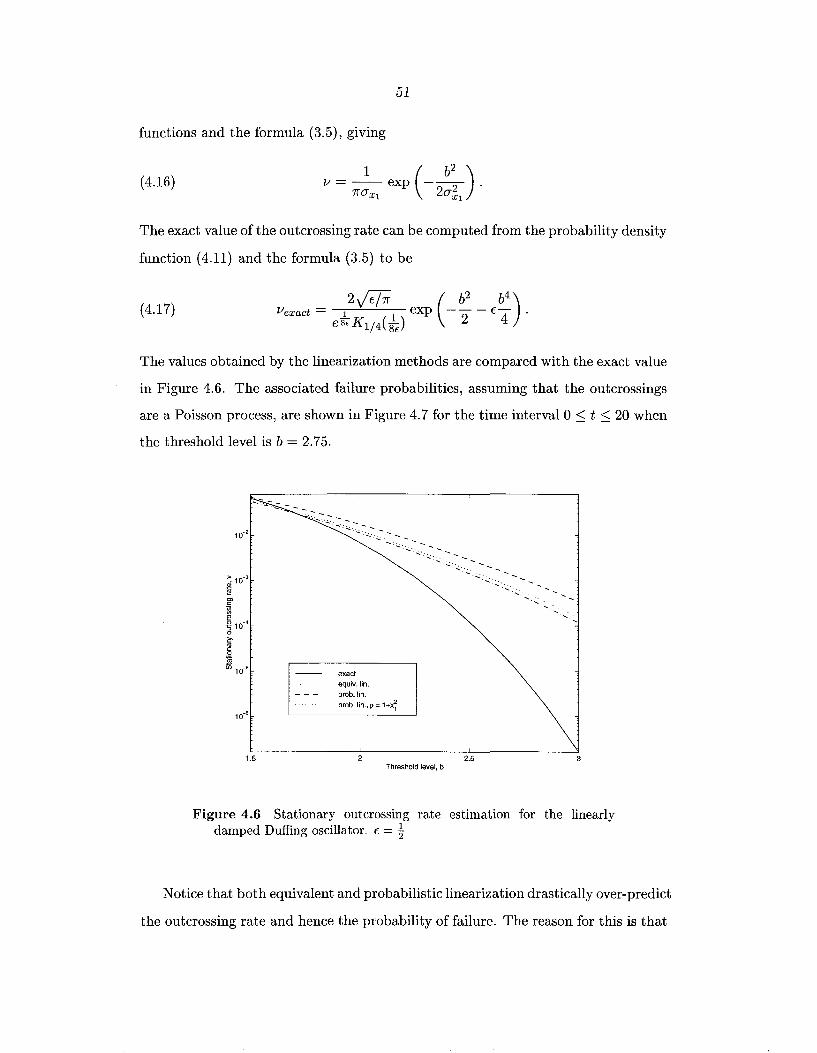
51

functions and the formula (3.5), giving

(4.16)

The exact value of the outcrossing rate can be computed from the probability density

function (4.11) and the formula (3.5) to be

(4.17)

The values obtained by the linearization methods are compared with the exact value

in Figure 4.6. The associated failure probabilities, assuming that the outcrossings

are a Poisson process, are shown in Figure 4. 7 for the time interval 0 ~ t ~ 20 when

the threshold level is b = 2. 75.

· .. : ....

1.5

exact equiv.lin. prob.lin.

·.:..: -·..:..·

·.....:.-.

prob. lin., p = 1 +>t,

2 Threshold level, b

:...:.·.· ·..:..·. - ...... :-.

· ... ::: . .....::~ · .

........ .........

2.5 3

Figure 4.6 Stationary outcrossing rate estimation for the linearly damped Duffing oscillator. E = ~

Notice that both equivalent and probabilistic linearization drastically over-predict

the outcrossing rate and hence the probability of failure. The reason for this is that

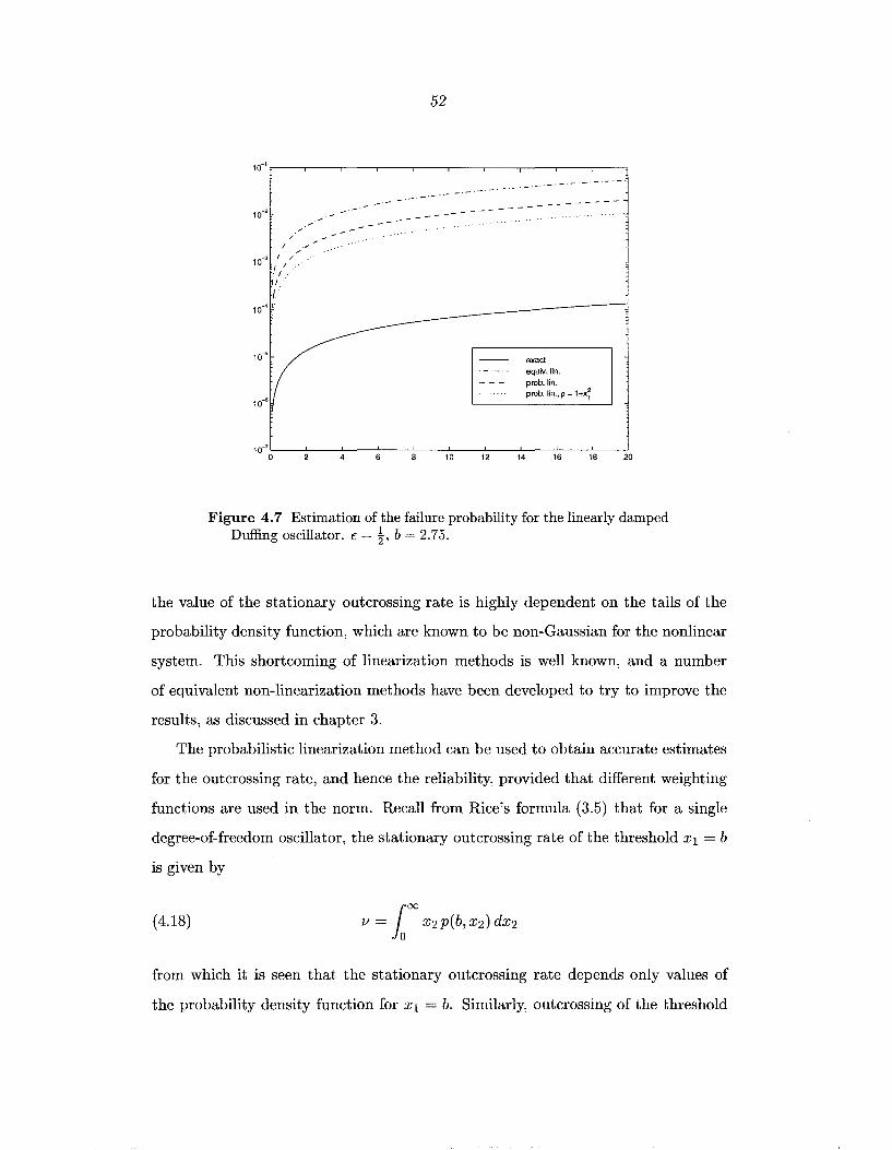
52

exact equiv.lin. prob. lin. prob. lin., p = 1 +X~

10-7 '----'-----'----'----'----'------'--'----'-----'--....J 0 4 6 8 10 12 14 16 18 20

Figure 4. 7 Estimation of the failure probability for the linearly damped Duffing oscillator. € = ~' b = 2.75.

the value of the stationary outcrossing rate is highly dependent on the tails of the

probability density function, which are known to be non-Gaussian for the nonlinear

system. This shortcoming of linearization methods is well known, and a number

of equivalent non-linearization methods have been developed to try to improve the

results, as discussed in chapter 3.

The probabilistic linearization method can be used to obtain accurate estimates

for the outcrossing rate, and hence the reliability, provided that different weighting

functions are used in the norm. Recall from Rice's formula (3.5) that for a single

degree-of-freedom oscillator, the stationary outcrossing rate of the threshold XI = b

is given by

(4.18)

from which it is seen that the stationary outcrossing rate depends only values of

the probability density function for XI = b. Similarly, outcrossing of the threshold

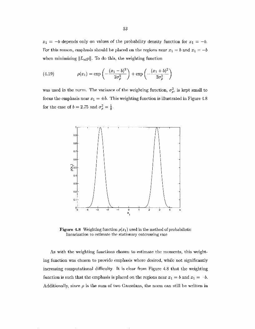
53

x 1 = -b depends only on values of the probability density function for x1 = -b.

For this reason, emphasis should be placed on the regions near x1 = b and x1 = -b

when minimizing IILnzPII· To do this, the weighting function

(4.19)

was used in the norm. The variance of the weighting function, a~, is kept small to

focus the emphasis near x1 = ±b. This weighting function is illustrated in Figure 4.8

for the case of b = 2.75 and a~ = k·

1\ 0.9

(\ 0.8

0.7

0.6

.:{"o.s 0..

0.4

0.3

0.2

) \ 0.1

0

) \ -5 -4 -3 -2 -1 0 3 4

x1

Figure 4.8 Weighting function p(xt) used in the method of probabilistic linearization to estimate the stationary outcrossing rate

As with the weighting functions chosen to estimate the moments, this weight­

ing function was chosen to provide emphasis where desired, while not significantly

increasing computational difficulty. It is clear from Figure 4.8 that the weighting

function is such that the emphasis is placed on the regions near x1 =band x1 = -b.

Additionally, since p is the sum of two Gaussians, the norm can still be written in

54

terms of polynomials times Gaussians, and can therefore be evaluated analytically.

With this choice of a weighting function, the method of probabilistic linearization

can be easily applied as before. The set of approximate probability density functions

is taken to be

and the probabilistic linearization criterion is

( 4.20)

where pis as in (4.19). Once the minimization in (4.20) has been performed to give

the optimal parameter 8-xu the estimate to the outcrossing rate is given by (4.16)

as

(4.21)

Estimates to the outcrossing rate obtained by this method are shown in Figure 4.9

for several values of the variance of the weighting function, a~. As expected, the

results improve as a~ decreases and for a~ = k the results are much better than

the equivalent linearization results given in Figure 4.6. However, if a~ is made too

small, a~ < k for this example, good estimates cannot be obtained by this method

for large values of b. The reason for this can be seen by examining the minimization

criterion in ( 4.20). The norm is given by

For most values of a~ the above integral is minimized by selecting O"x 1 so that

55

over the regions near x1 =±b. But, as O"~ becomes small small and b becomes large,

the minimum achieved by having O" x 1 satisfy the above condition becomes a local

minimum, and a global minimum is achieved at a value of O"x1 very near zero. In

this case, the local minimum can still be found by standard minimization techniques

and is of use, but the global minimum, which gives a corresponding outcrossing rate

approximation very near zero, is of no use. In order to obtain the most accurate

estimates for the outcrossing rate, O"~ should be kept small so that emphasis is given

to regions near x1 = ±b, but not so small that the optimal value of O" x 1 goes to zero.

Such a value of O"~ can be found by starting with a relatively large value for O"~ and

reducing O"~ until no reasonable results can be obtained.

"' <: =~"""'"'~"'',·: "'' ~, -. '·,, '-o...

10-3 ...................... - e- -G.

'·

-e- prob. lin., wtd. norm with

10-5 prob. lin., wtd. norm with

prob. lin., wtd. norm with

prob. lin., wtd. norm with

10-6 exact

0"2=5 p

cr2 = 1 p

a!= 1/3

a2 = 1/8 p

'· '· ·,,

' '

'·

' '

'· '· '·

' ' '

'·

' '

'·

' '

'· '·

' ' '

10-''---------'---------'----------' 1.5 2 2.5

b

Figure 4.9 Stationary outcrossing rate estimation for the linearly damped Duffing oscillator using weighted norm, where the weighting function is as in (4.19). t: = ~·

56

4.2.2 Other Interpretations of the Probabilistic Linearization Cri­

terion

In the probabilistic linearization method outlined in section 4.2, a linear system

is found whose corresponding probability density function best approximates the

Fokker-Planck equation corresponding to the nonlinear equation. Letting Lnz(x)

and Ltin(x) be the forward Kolmogorov operators for the nonlinear system (4.1)

and the linear system (4.6), respectively, the associated stationary Fokker-Planck

equations are

(4.23)

(4.24)

Lnz(x)pnz(x)

Ltin(x )Plin(xiB)

0

0.

The probabilistic linearization criterion ( 4.8) can then be written as

min IILnz(x)Plin(xiB) - Ltin(x)Plin(xiB) II I:IE6

which is in a form similar to the equivalent linearization criterion (3.9).

Also, by choosing a different norm, this approach can be viewed as minimizing

the solution error. Define a norm on P by

(4.25) lifliL~zLnl = { f(x)L~z(x)Lnz(x)f(x) dx }fRn

;here L~1 , the adjoint of Lnz, is the backward Kolmogorov operator defined by

(2.23). The norm in (4.25) is just £} norm weighted with the operator L~zLnl·

The operator L~zLnz is self-adjoint and is positive definite on P (provided the exact

solution to the Fokker-Planck equation is not in P, in which case it is only positive

semi-definite), so that (4.25) actually defines a norm.

In this norm, the criterion ( 4.8) is equivalent to

min IIPnz(x)- Plin(xiB)IIL* L I:IE6 nl nl

since

57

IIPnl- Pliniii~1 Lnl = ((Pnl- Plin), L~lLnl (Pnl- Plin)) £_2

= (Lnl (Pnl - Plin) , Lnl (pnl - Plin)) £_2

where(·, ·)c_2 is the standard inner product on £ 2 .

(eq. 4.25)

(eq. 4.23)

This shows that in the norm defined by ( 4.25), the probabilistic linearization

criterion can be viewed as minimizing the difference between the approximate prob­

ability density function and the exact (unknown) probability density function.

4.2.3 Comments on Applicability to Multi-Degree-Of-Freedom Sys-

terns

Example 1 illustrated the applicability of the method of probabilistic linearization

to a single degree-of-freedom oscillator. The method is also applicable to multi­

degree-of-freedom systems. As in the case of the single degree-of-freedom oscillator,

for polynomial-type nonlinearities, the norms can be evaluated analytically since

they will still involve computing moments of a Gaussian process. The problem is

then to obtain the elements of the covariance matrix which minimizes the norm, i.e.

to solve a p-dimensional minimization problem. The dimension p is the number of

elements in the covariance matrix. For a general n-dimensional nonlinear system,

this would yield

n(n + 1) p = ___:__ _ ___:_ 2

unknown elements of P, since P is symmetric. In many cases, this number can be

reduced since some of the elements of P are usually known; for example, E[xixi] = 0

for all i. Thus, obtaining an approximate stationary probability density function

by the method of probabilistic linearization for an n-dimensional nonlinear system

58

requires solving a minimization problem in at most n(n2+1

) dimensions.

4.3 Probabilistic Nonlinearization

In the previous section, the probability density function for the nonlinear system of

interest was approximated by the probability density function for a linear system.

For linear systems, the probability density function is known to be Gaussian, and

the Fokker-Planck equation associated with the linear system can easily be solved

for the probability density function. Since the response of nonlinear systems is

known to be non-Gaussian, it is of interest to see what type of improvement can

be obtained by approximating the solution to the Fokker-Planck equation with a

non-Gaussian probability density function. In this section, the nonlinear system of

interest will be replaced by a different nonlinear system having a known solution to

the Fokker-Planck equation. The probability density function for the response of

the "simpler" nonlinear system will then be taken as the approximate probability

density function for the nonlinear system of interest.

As mentioned earlier, there are very few nonlinear systems in more than two

dimensions having known solutions to the stationary Fokker-Planck equation. For

this reason, the method presented in this section will be limited to approximating

the probability density function for single degree-of-freedom nonlinear oscillators of

the form

(4.26)

The stationary Fokker-Planck equation associated with (4.26) is

( 4.27)

As discussed in section 3.1, for nonlinear systems subjected to additive stochastic

excitation, many of the known solutions to the Fokker-Planck equation are for single

degree-of-freedom oscillators with energy-dependent damping. As in the method of

59

equivalent nonlinearization (section 3.3.2) the probabilistic nonlinearization method

approximates the nonlinear system of interest ( 4.26) by a system of the form

( 4.28) (

dxl(t)) ( x2 ) ( 0 ) = dt + dw(t) dx2(t) - feqnl(H) X2- g(xl) ../2J5

where His the Hamiltonian, defined by (3.2). The solution to the stationary Fokker­

Planck equation associated with (4.28) is, from (3.3),

While the equivalent nonlinear function feqnl(H) can be chosen to be of any

form, a simple choice is to choose a power series in H

for some p E z+, giving

p

feqnl(HIO) = L eiHi-l i=l

( 1 P Hi(x))

Peqnl(xiO) = aexp - D ?=ei -z-.- . z=l

The number of terms included in the power series is chosen based on the properties

of the function f(xl, X2)· The parameters, e, of feqnl(HIO) can then be determined

so that the probability density function associated with the nonlinear system (4.28)

minimizes the Fokker-Planck equation error

min II Lnl(X)Peqnl(xiO) II·

As in the probabilistic linearization method, the step of finding the equivalent non­

linear system (4.28) will be bypassed and the probability density functions will be

approximated directly. The set of approximate probability density functions is cho-

60

sen as

- 2 2 . - 1 H~ (X) p

{ (

p . ) } (4.29) PH - Peqnl E C (lR ) . Peqnz(xJO) - aexp - D t; Oi -2-. - , 0 E lR .

Note that given any Peqnl E PH, Peqnz(xJO) is only a function of H(x) and can

be therefore be written in the form Peqnz(xJO) = h(H(x)JO), giving

8peqnl = 8h 8H =g(xi) 8h 8x1 8H 8x1 8H

8peqnl 8h 8H 8h ax2 aH ax2 x 2 aH

so that

and the error in the stationary Fokker-Planck equation (4.27) is reduced to

(4.30)

The probabilistic nonlinearization criterion is then

or,

(4.31)

min II Lnz(x)p(x) II pEPH

min II Lnz(x)Peqnz(xJO) II. OEIRP

While (4.31) is a valid criterion, finding the optimal parameters would require

a significant amount of computation since evaluating the norm requires a two­

dimensional numerical integration, and performing the minimization would require

computing the norm several times. In the next section, some simplifications to

(4.31) will be made which will significantly reduce the computational burden.

61

4.3.1 Simplifications of the Probabilistic Nonlinearization Crite-

rion

It was mentioned above that finding the optimal parameters for the probabilistic

nonlinearization criterion (4.31) requires a number of two-dimensional numerical

integrations. To enable computations to be done efficiently, two simplifications will

be made.

First, a somewhat simpler expression than IILnzPeqnlll is minimized. Substituting

(4.30) into (4.31) gives the criterion

( 4.32)

The first simplification made is that instead of minimizing the derivative of the

quantity in parenthesis, the quantity itself is minimized, i.e.

( 4.33) . II ( ) ( IB) apeqnz(xiB) II mm f XI' X2 Peqnl X + D a 0

BE~P X2

The derivative of Peqnl with respect to x2 can easily be evaluated, giving

apeqnl(xiB) __ ...!._ (~ B·Hi-1) ( IB) a - D L.J ~ X2 Peqnl X 0

X2 i=l

Substituting into ( 4.33) gives

which, using the standard £ 2 norm, is

( 4.34)

Notice that this criterion is virtually identical to the criterion used by the method of

equivalent nonlinearization (section 3.3.2); the equivalent nonlinearization criterion

(3.22) is the same as (4.34) withp;qnl replaced by Peqnl· While this first simplification

62

has simplified the form of the criterion from (4.32) to (4.34), the resulting integral

still cannot be evaluated analytically for most systems.

The second simplification comes in evaluating the integral in ( 4.34). As it is

written, evaluating the integral requires a two-dimensional numerical integration. To

allow analytical computation of the integral, Peqnz(xiO) is replaced in the integral by

Plin(x1,x2) obtained by the method of probabilistic linearization. This is equivalent

to using the weighting function

in the norm. The probabilistic linearization method can be very efficiently applied,

and making this substitution will enable the optimal parameters to be computed

very efficiently.

Thus, after the two simplifications, the probabilistic nonlinearization criterion

becomes

(4.35)

Now, (4.35) can be easily minimized with respect to e. To find the minimum, set

k = 1, 2, ... ,p.

Evaluating the derivatives gives a linear equation for the optimal parameters 0

( 4.36) AB= b.

The matrix A E iRPXP and vector bE !RP are given by

Aij (Hi-lx2, Hi-lx2)

bi (!, Hi-lx2)

63

where the inner product is defined by

(4.37)

With the optimal parameters known, the approximate probability density function

is then given by

( 4.38) (

1 P ~Hi(x)) Peqnz(x) = aexp - D '?=Bi-~-·- .

t=l

A chart outlining the steps for the method of probabilistic nonlinearization is

given in Figure 4.10. Notice that before obtaining the approximation Peqnz(x), the

probabilistic linearization approximation Plin(x) is obtained. The relative accu­

racy of the two approximations can be compared by computing IILnz(x)Plin(x)ll and

IILnz (x)Peqnz(x) II·

4.3.2 Example 2: Nonlinearly Damped Duffing Oscillator

To illustrate the method, a nonlinearly damped Duffing oscillator is considered.

This oscillator has been previously studied by Elishakoff and Cai (1993).

(4.39) = dt + dw(t) (

dxl(t)) ( x2 ) ( 0 ) dx2 ( t) - f3x2 - ax~ - '}'Xl - cxi VW

In the notation of ( 4.26),

giving

f3x2 +ax~ . 3

'}'Xl + EX1

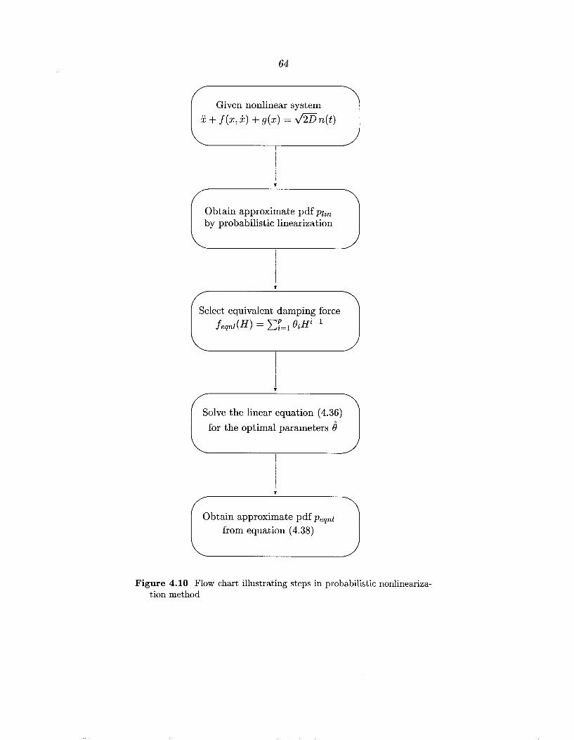
64

Given nonlinear system

x + f(x,x) + g(x) = v'2i5n(t)

Obtain approximate pdf Plin by probabilistic linearization

Select equivalent damping force feqnl(H) = l:f=l (}iHi-l

Solve the linear equation ( 4.36)

for the optimal parameters iJ

Obtain approximate pdf Peqnl from equation (4.38)

Figure 4.10 Flow chart illustrating steps in probabilistic nonlineariza­tion method

65

As in (4.29), the equivalent system is chosen by replacing f(xl, x2) with feqnl(HjO)x2

where feqnl(HIO) is a power series in H. Since

it seems reasonable to approximate this function by the following power series

The series is truncated at order H so that the highest power of x2 in the equivalent

damping term feqnz(H)x2 is the same as the highest power in the original system

The set of approximate probability density functions is then

The set of linear equations ( 4.36) for the optimal parameters is given by

(4.40)

where the inner product is as in ( 4.37).

All of the quantities in ( 4.40) involving ( ·, ·) can be evaluated once Plin has been

computed by the probabilistic linearization method. With these quantities known,

(4.40) is a linear system of equations in the two unknowns fh and {h, which can

be easily solved. Once iJ1 and iJ2 are known, the approximate probability density

function is given by

A ( fjl {h 2 ) Peqnl(xiO) = aexp - DH(x)-2DH (x) .

All of the integrals up to this point can be done analytically. Evaluating the normal­

ization constant a and other quantities such as moments and expected outcrossing

66

rates requires numerical integration.

In order to compare this method with some of the other methods presented

earlier, two different cases are considered. First, all of the parameters except for the

coefficient E of the nonlinear stiffness term are fixed, and the approximate probability

density function are computed for various values of E. The resulting mean square

values are shown in 4.11 and the errors in the Fokker-Planck equation are shown in

Figure 4.13. In the other case, all of the parameters except for the coefficient a of

the nonlinear damping term are kept fixed, and the approximate probability density

functions are obtained for various values of a. The mean square values are shown

in Figure 4.12 and the Fokker-Planck equation error in Figure 4.14. In all cases, it

is seen that the probabilistic nonlinearization provides more accurate results than

the linearization or partial linearization results. The simulation results presented in

Figures 4.11 and 4.12 are from Elishakoff and Cai (1993).

The approximate probability density functions obtained by the methods are also

plotted. Figures 4.15-4.18 show the probability density functions as both surface

plots and contour plots. The marginal probability density functions for XI and x2

defined by

p(xi) I: p(xi, x2) dx2

I: p(xi,x2) dxi

are shown in Figures 4.19 and 4.20. In these plots, the marginal probability density

functions for various approximate methods are compared with histograms of the

response obtained by numerical simulation of the system; 400,000 points were used

to make the histograms. Although the probabilistic nonlinearization method gives

good approximations to the mean square values and provides a good approxima­

tion to the probability density function p(x2), it is seen that the probability density

function p( XI) obtained by the method of probabilistic nonlinearization decays much

more rapidly as lxii increases than the simulation results or the other approximate

methods. It will be seen in section 4.4.3 that this leads to large errors when ap-

67

1.2 r.-, -;---r------r--------,--,----r;::::==:::!::==::!:::==::::::===='===~ lj I

1 I 1,1 '.·1 I

01 :\. I 'I I ·,·1 I

':\X I 0.9 .. 1 I

:I

0.8

"'~ >< 0.7 w

0.6

0.5

0.4

0.3

0

' ' X

0 ·-.... X

0

X

0

prob. lin., p = 1+x~ x~ simulation

prob. nonlin.

prob. lin., p = 1+x~ partial lin.

equiv.lin

10

Figure 4.11 Mean square values as a function of the stiffness nonlinear­ity for the nonlinearly damped Duffing oscillator ( 4.39). D = n, a =

0.5, ,B = 0.1, ')' = 1.

1.3

1.2 \

\

1.1 ¥

0

"~ X 0.9 tiT

' ' Q

0.8

0.7

0.6

0.5

'

\

'

' '

o" ......

' ' X '-

....:· .. 0 -.

0

68

X

'·"':-,. __

0

0 0 ···· ...

0 0

X

0

0 0 0

prob. lin .• p ~ 1 +;,' x~ simulation

prob. nonlin.

prob. lin .• p ~ 1 +x~ partial lin.

equiv.lin

······· .... 0 ········

0·4oL_ __ o_,_.1 __ _,o.~2--o-'-.3---'0.-4--0.L.s--o--'.s---oL.7--0...I..s ___ oL.9-__j

a

Figure 4.12 Mean square values as a function of the damping nonlinear­ity for the nonlinearly damped Duffing oscillator ( 4.39). D = 1r, j3 = 0.1, E = 1, f' = 1

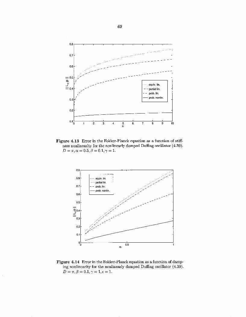
69

0.8 r----.-----.--..------.-----,--,...--...,--~--,...-~

0.7

0.6

/ == 0.5 .. ~-/ a. ."/ "2 I

...J

= 0.4

0.3 f.; I

0.2

I I

/

/

/

. ' . . . . . . . . . . ' . . . . . . . . . . .

--- ---

· · · · · equiv. lin .

·- · - partial lin.

- - prob. lin.

- prob. nonlin.

L-----------------1 2 3 4 5

E 6 7 8 9 10

Figure 4.13 Error in the Fokker-Planck equation as a function of stiff­ness nonlinearity for the nonlinearly damped Duffing oscillator (4.39). D = 1r,a = 0.5,(3 = 0.1,"( = 1.

0.9,-----------,-------------.,.,

0.8

0.7

0.6

0.5

= '::0.4

.... I'

0.3

0.2

0.1

·· equiv.lin.

·- ·- partial lin.

- - prob. lin.

- prob. nonlin.

.· ,.· .··_,.·

.· ·"' .·· /

.. ··_/· // .· .///

.. -~:. / 4

. _,.·

. _,..· .· /

0.5 a

Figure 4.14 Error in the Fokker-Planck equation as a function of damp­ing nonlinearity for the nonlinearly damped Duffing oscillator ( 4.39). D = 1r,(3 = 0.1,"( = 1,€ = 1.

70

proximating the outcrossing rate for this system. Further results for this example,

including outcrossing rate estimates, will be given in section 4.4.3.

0.14

0.12

0.1 -><~.08 ><~06 a:·

0.04

0.02

0

-2

2

1.5

0.5

><C\J 0

-0.5

-1

-1.5

-2

Figure 4.15 Stationary probability density function approximation ob­tained by the method of equivalent linearization for the nonlinearly damped Duffing oscillator. a= 0.5, ,8 = 0.1, 'Y = 1, E = 1.

4.4 Direct Approximation of the Probability Density

Function

The previous methods presented approximated the nonlinear system of interest with

a different system for which the corresponding Fokker-Planck equation function can

be solved. As discussed earlier, there are relatively few systems which have a known

71

-2

2

1.5

0.5

><C\J 0

-0.5

-1

-1.5

-2

Figure 4.16 Stationary probability density function approximation ob­tained by the method of partial linearization for the nonlinearly damped Duffing oscillator. a = 0.5, f3 = 0.1, 'Y = 1, E = 1

0.14

0.12

0.1

72

-2

2

1.5

0.5

XC\J 0

-0.5

-1

-1.5

-2

Figure 4.17 Stationary probability density function approximation ob­tained by the method of probabilistic linearization for the nonlinearly damped Duffing oscillator. a: = 0.5, ,B = 0.1, 'Y = 1, € = 1.

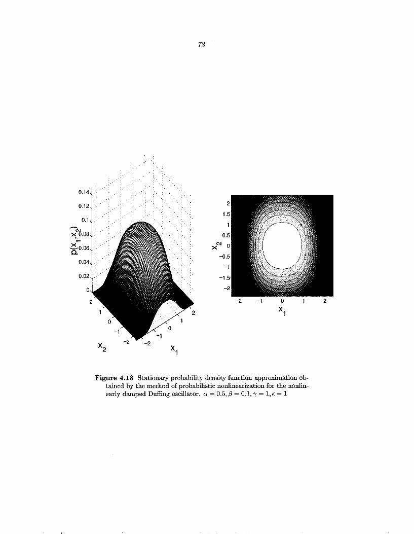
0.14

0.12

0.1 -x"6.oa ..-

>< 0 06 c:· 0.04

0.02

0

73

.. 2

1.5

0.5 C\1

>< 0

-0.5

-1

-1.5

-2

-2 -1 0

x1

-2

Figure 4.18 Stationary probability density function approximation ob­tained by the method of probabilistic nonlinearization for the nonlin­early damped Duffing oscillator. a= 0.5, {3 = 0.1, 1 = 1, E = 1

2

0.5

0.4

/.

~ 0.3

0.2

0.1

74

' /

:/ J

i ~-

' '·. , .. \

\ '.\ ',I

'· · .. I

~ ... ,~ '~ · .. \

· .. [\'

-\ ·~ . . I \ . I .

prob. nonlin. partial lin. prob.lin. equiv. lin

Figure 4.19 Probability density function p(xl) for the nonlinearly damped Duffing oscillator for the various approximation methods. The histogram shows results from numerical simulation of the sys­tem.

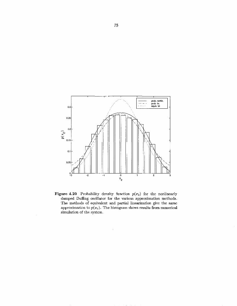
N X

0:

0.3

75

prob. nonlin. prob.lin. equiv.lin

Figure 4.20 Probability density function p(x2) for the nonlinearly damped Duffing oscillator for the various approximation methods. The methods of equivalent and partial linearization give the same approximation to p(x2). The histogram shows results from numerical simulation of the system.

76

solution to the Fokker-Planck equation, and a given nonlinear system may not be

well approximated by any of the solvable nonlinear systems. In this case, the set of

approximate probability density functions can be chosen to be of a different form,

where the form is chosen based on knowledge of the system.

In this section, another method is presented for obtaining non-Gaussian proba­

bility density functions to approximate the solutions to the stationary Fokker-Planck

equation for a given nonlinear system. Unlike section 4.3, the approximate prob­

ability density functions are not chosen to correspond to solutions of "equivalent"

systems with energy-dependent damping. In fact, the approximate probability den­

sity functions chosen are such that no equivalent system

may exist whose stationary probability density function is of the form of the ap­

proximate probability density functions.

4.4.1 Selecting the Approximate Probability Density Functions

This section presents a method for selecting the set of approximate probability

density functions for single degree-of-freedom systems. The approximate probability

density functions are chosen with two objectives in mind. First, the approximate

solutions are chosen so that some of the terms in the Fokker-Planck equation error

are identically zero. Additionally, the form of the approximate solutions is chosen so

that if the given system is one of the systems having a known solution to the Fokker­

Planck equation, the approximate method will actually give the exact solution.

For a given nonlinear dynamical system

77

the associated stationary Fokker-Planck equation is

which can be rearranged as

ap ap a( ap) -x2-a +g(xi)-a +-a J(xi,x2)p+D-a =0. XI X2 X2 X2

The term in parenthesis will be identically zero if

which is accomplished by choosing

( 4.41)

where Q(xi) is an arbitrary function of XI, ()is a parameter to be determined, a is

a normalization constant and

The form of the function Q(xi) is chosen based on systems having known so­

lutions to the Fokker-Planck equation. A desirable property for an approximation

method is to be able to give the exact solution for systems having known solutions.

An attempt is made to choose Q(x1) so that the approximate method will actu­

ally yield the exact solution for systems with known solutions to the Fokker-Planck

equation. With this in mind, one of the simplest choices for Q(xi) is to choose

(4.42)

which would yield the exact solution in the case of linear damping. This is the

choice considered in the examples. A slightly more complicated choice for Q(x1)

78

can be chosen which will yield the exact solution for any system having energy­

dependent damping, as explained in appendix A. For the examples considered in

this work, in which j(x1, x2) is independent of x1, this alternative choice also gives

Q(x1) = G(x1).

With Q(xl) given by (4.42), the set of approximate probability density functions

is given by

and the criterion for obtaining the best approximation is given as

( 4.43)

As in the case of probabilistic nonlinearization, this provides a valid criterion for

measuring the error, but can be computationally expensive to work with. For typical

systems, computing the norm requires numerical integration, and to find the optimal

parameters, the integration needs to be performed many times.

To simplify the criterion, recall that the set Pp was chosen so that

Therefore, the Fokker-Planck equation error reduces to

Part of the difficulty in minimizing the norm of the above expression is that the

normalization constant for the probability density function pp(xiB) is a complicated

function of 0. To simplify the computations, the following criterion is adopted

(4.44)

79

Differentiating with respect to (} to obtain the minimum gives

(4.45) (} = E[g2(x1) j(x1, X2) X2- g(xi) X2 Bf;J

E[g2 (xt) x~]

Although this criterion seems different than the other methods presented in this

chapter, it can be thought of as minimizing the weighted £ 2 norm of the Fokker­

Planck equation error where the weighting function is 1jpp(xl0). An interesting

relationship between the criterion ( 4.45) and those suggested by the methods of

equivalent and partial linearization is presented in section 4.5.

Notice that if j(x1, x2) is independent of x1, the criterion reduces to

(4.46) (} = E[x2 j(x2)] E[x~]

which is the same as the criterion proposed in the methods of equivalent linearization

(3.10a) and partial linearization (3.20). The only difference in the criteria is that

different probability density functions are used to evaluate the expectations.

4.4.2 Example 3: Rolling Ship

For small angles, the equation of motion for a rolling ship is given by (Roberts 1982;

Gawthrop et al. 1988)

where ¢ is the angle from the vertical, w is the undamped natural frequency for

roll, f3 is the linear damping ratio, n1 and n2 are nonlinear damping and stiffness

coefficients, respectively, I roll is the effective roll inertia of the ship, and M ( t) is the

applied moment from the waves. The equation contains a quadratic damping term

commonly found in applications involving fluid flow or fluid dampers as well as a

80

cubic hardening term. Modeling M(t) as Gaussian white noise leads to

(4.47)

where x1 = ¢, x2 = ¢ and D is the amplitude of the excitation.

For the system ( 4.4 7),

giving

81

The approximate probability density function is taken as

where, from ( 4.46),

(4.48) () _ E[x2 j(x2)]

- E[x§]

The effects of the cubic stiffness nonlinearity have already been investigated,

and in to obtain some simple analytical results for the nonlinear damping term, the

first case considered is {3 = n2 = 0 and w = 1 so that the system reduces to the

quadratically damped oscillator

(4.49)

The more general case will be studied in section 5.2.2. For the quadratically damped

oscillator (4.49), the approximate probability density function is

(4.50) ( ) ( ()xi n1x§lx2l)

p F x = a exp -- - ---==-----'-2D 3D

and, from ( 4.48), () is given by

(4.51)

where r(-) is the Gamma function.

The mean square values can easily be determined from the probability density

function

2 2 (3D) ~ 1 ( D ) ~ E[x1] = E[x2] = - -(1 ) = 0.776 - . nl r 3 nl

The error in the Fokker-Planck equation can also be computed analytically; in

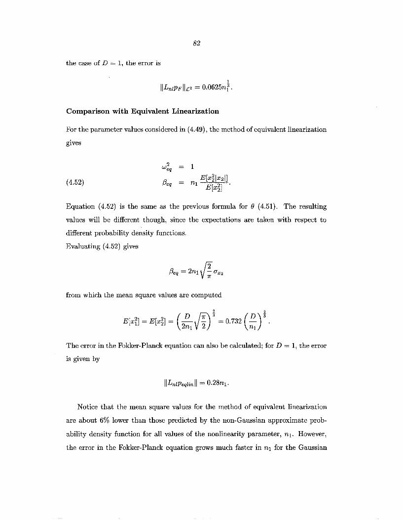
82

the case of D = 1, the error is

1

IILnlPF llc2 = 0.0625n{.

Comparison with Equivalent Linearization

For the parameter values considered in ( 4.49), the method of equivalent linearization

gives

( 4.52)

Equation (4.52) is the same as the previous formula for (} (4.51). The resulting

values will be different though, since the expectations are taken with respect to

different probability density functions.

Evaluating ( 4.52) gives

from which the mean square values are computed

The error in the Fokker-Planck equation can also be calculated; forD= 1, the error

is given by

IILnlPeqlinll = 0.28n1.

Notice that the mean square values for the method of equivalent linearization

are about 6% lower than those predicted by the non-Gaussian approximate prob­

ability density function for all values of the nonlinearity parameter, n1. However,

the error in the Fokker-Planck equation grows much faster in n1 for the Gaussian

83

approximation than for the non-Gaussian approximation.

Comparison with Equivalent N onlinearization

The quadratically damped oscillator is one of the systems for which the integrals

arising in the equivalent nonlinearization method can be analytically evaluated, and

the results can be presented in a simple form. The solution presented here is taken

from Roberts and Spanos (1990). The nonlinear damping term j(x2) = n1lx2lx2 is

replaced with an "equivalent" nonlinear damping given by

where H =~(xi+ x~) and a is chosen to solve

In Roberts and Spanos (1990), the optimal value for a is determined and the

corresponding probability density function for the equivalent nonlinear system is

given by

( 4.53) _ 3 8n1 8n1 3/2

( )2/3 ( )

Peqnl(x) - 27!T(~) 97r exp - 97r (2H(x)) .

The mean square values can be computed from (4.53) and are given by

which are a little more than 1% lower than those predicted by the probability density

function in equation ( 4.50). The mean square values for the various methods are

plotted in Figure 4.22 along with values obtained by numerical simulation.

The error in the Fokker-Planck equation is computed by numerical integration

and is plotted in Figure 4.21. While the equivalent nonlinearization method provides

a better fit than equivalent linearization, the error still grows much faster in n 1 for

84

the equivalent nonlinearization method than the new method.

The marginal probability density functions p(xl) and p(x2) for the various meth­

ods are shown in Figures 4.23 and 4.24, along with histograms obtained from nu­

merical simulation of the system. Eight hundred thousand data points were used to

make the histograms. From both figures, it is seen that the non-Gaussian probabil­

ity density functions provide a better fit to the simulated data than the equivalent

linearization results, and it appears as though the best fit to the simulated data is

obtained by using the direct approximation of the probability density function.

0.6.------------,---------------,

·· · · · equiv.lin

0.5 - - equiv. nonlin.

- pdf approx.

0.4

0.2

0.1

2

Figure 4.21 Fokker-Planck equation error for the quadratically damped oscillator with D = 1.

Reliability Estimates for the Various Methods

The mean square values and Fokker-Planck equation errors for the various methods

were presented in Figures 4.21 and 4.22. It was seen that all of the methods gave

quite good accuracy for the mean square values for all values of n1, but that the

1.2 \ \

\ ·. \

1.1 · .. \

=0.9 a. c

_J

=o.8

0.7

0.6

0.5

0.6

'

0.8

' X ' '

85

' X '

1.4

equiv.lin

equiv. nonlin.

- pdf approx.

x simulation

1.6 1.8

Figure 4.22 Mean square values for the quadratically damped oscillator with D = 1.

><~

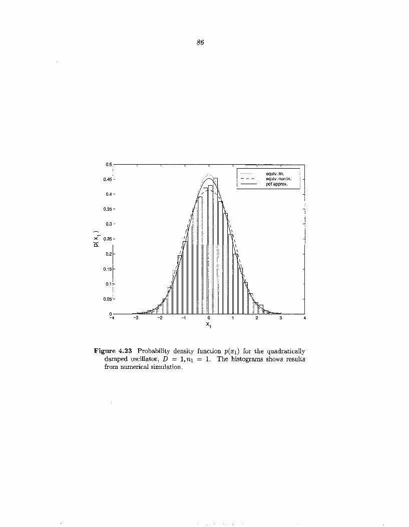
0:

0.5

0.45

0.4

0.35

0.3

0.25

0.2

0.15

0.1

0.05

0 -4

~·

~: -3 -2

1 I

I

I~ I

If I

I

r! 1.'

-1

86

equiv.lin.

/:_· --- equiv. nonlin.

I 1\ -- pdf approx.

I 'I~

~ \

1~\ \ \

A\ \ \

r; \ ·\

I\ ~

~

~ 2 3 4

Figure 4.23 Probability density function p(xl) for the quadratically damped oscillator, D = 1, n1 = 1. The histograms shows results from numerical simulation.

C\1 X

c::

0.5

0.45

0.4

0.35

0.3

0.25

0.2

0.15

0.1

0.05

0 -3

.. Alfl -2

87

..

/ ...... --,

r-... v

17 ~

~l I·

j ... I

~ .. · 1.

~ .. ·

-1

. . . . . . . . equiv.lin. --- equiv. nonlin. -- pdf approx.

'· . r"· ~

~-~ ·.I

·1A I

··[~ I

··r~ ·.lA

·~ ·· .....

2 3

Figure 4.24 Probability density function p(x2 ) for the quadratically damped oscillator, D = 1, n1 = 1. The histogram shows results from numerical simulation.

88

error in the Fokker-Planck equation was much smaller for the probability density

function PF than for the equivalent linearization or nonlinearization methods. In

this section, the outcrossing rates for the various methods are compared.

In addition to the previously described methods, results are presented from a

weighted norm minimization. In this case, the probability density function is chosen

as

as in (4.50), but rather than choosing e according to (4.46), e is chosen to minimize

the weighted £ 2 norm of the Fokker-Planck equation error. As in the reliability

estimation for probabilistic linearization, the weighting function is chosen as

As in example 1, the value of O"p was reduced until the results suddenly became

unreasonable, corresponding to the optimal value of 0 going to oo. The smallest

value of O"p which could be used in this example is O"~ = ~-

The results for the various methods are shown in Figure 4.25, along with results

obtained from numerical simulation of the system. It is seen that the equivalent

nonlinearization method predicts the outcrossing rate to be much lower than what

is predicted by the other methods. The reason for this is that the outcrossing rate

decays as e-c1 b3

for some constant c1 for the equivalent nonlinearization method

whereas the outcrossing rate for the other methods decay as e-c2 b2

•

Note that these results illustrate an important point about equivalent nonlin­

earization methods. The results obtained by equivalent nonlinearization may be

less accurate than those obtained by equivalent linearization if the approximate

nonlinear system has sufficiently different behavior than the original nonlinear sys­

tem. This can be seen in Figure 4.25, where the method of equivalent linearization

gives considerably better estimates to the outcrossing rates than those obtained by

equivalent nonlinearization for this system.

X

1.5

equiv.lin. pdf. approx.

89

wtd. norm method, rl = 0.5 equiv. nonlin. P

simulation

2 2.5 Threshold level, b

' ' ' ' ' '

3

' ' ' ' '

'

' ' ' ' ' ' ' ' ' 3.5

Figure 4.25 Expected outcrossing rates for the quadratically damped oscillator. n 1 = 1, D = 1.

90

4.4.3 Application of the Method to Example 2

It was seen in section 4.3 that the probability density function obtained by the

method of probabilistic nonlinearization provided a considerably better fit to the

stationary Fokker-Planck equation for the nonlinearly damped Duffing oscillator

than either the method of equivalent linearization or probabilistic linearization. It is

interesting to see how the results obtained by probabilistic nonlinearization compare

with the results obtained by approximation the probability density function as in

section 4.4.1.

For the nonlinearly damped Duffing oscillator given by ( 4.39),

j(x2) f3x2 +ax~

g(xr) = ')'XI + EXf

giving

G(x1)

The probability density function is given by

(4.54)

where, from (4.46),

which can be evaluated as

O = 8aD K ~ ( sfo) + (32 ( K ~ ( sfo) - K! ( sfo))

2(3 ( K ~ ( 8~~) - K i ( /ln))

where Kn(·) are modified Bessel functions. The Fokker-Planck equation error,

91

IILnz(x)p(xiO)II is compared with the error for the methods presented earlier in

Figures 4.26 and 4.27. It is seen that the direct approximation of the probabil­

ity density function provides a better fit to the Fokker-Planck equation than any

of the other methods. The mean square values obtained by the various methods

are shown in Figures 4.28 and 4.29. From these plots, it is seen that both of the

nonlinearization methods do considerably better than the linearization methods.

The stationary probability density function PF is shown in Figure 4.30 and can be

compared to those obtained from the various other methods, which are shown in

Figures 4.15-4.18. The marginal probability density functions, p(x1 ) and p(x2 ), are

shown in Figures 4.31 and 4.32. The approximate probability density functions are

compared with results from numerical simulation, as in Figures 4.19 and 4.20.

0.8,----.----.----.--.----.----.---,--..,--....,.---,

0.7

0.6

0.5 . .::...

a. c 0.4

-'

./

1

I

0.3 ,'

0.2

/ /

--- ---

0

equiv.lin. partial lin. prob.lin. prob. nonlin. pdf approximation

~1 ooooooooooooooooooooooooo toooooooo

4 7 &

10

Figure 4.26 Error in the Fokker-Planck equation as a function of stiff­ness nonlinearity for the nonlinearly damped Duffi.ng oscillator (4.39). D = 1r,o: = 0.5,,8 = 0.1,')' = 1

The most striking difference between the method of probabilistic nonlineariza­

tion and the direct probability density function approximation method appears when

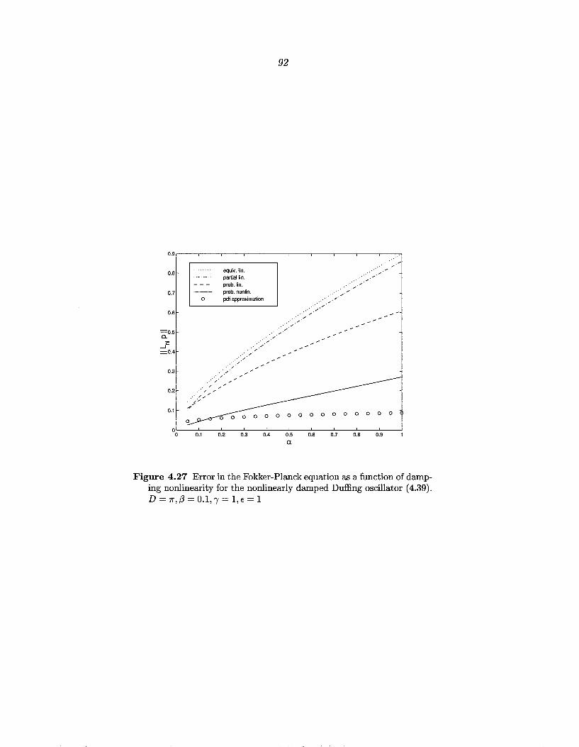
92

0.9,----,---,----,---,----,---,----,------,,----,---,

0.8

0.7

0.6

=o.s a. _]= =0.4

0.3

0.2

0.1

0

equiv.lin. partial lin. prob.lin. prob. nonlin. pdf approximation

. / .·_,.· ·_;

.· ·"" .· ·"'

0 0 0 0 0 0 0 0

00L--~-~0L.2-~0L.3-~0L.4-~0L.5-~0.L6-~0.L7-~0.L8-~0.L9-~

a

Figure 4.27 Error in the Fokker-Planck equation as a function of damp­ing nonlinearity for the nonlinearly damped Duffing oscillator (4.39). D = rr,/3 = 0.1,'}' = 1,E = 1

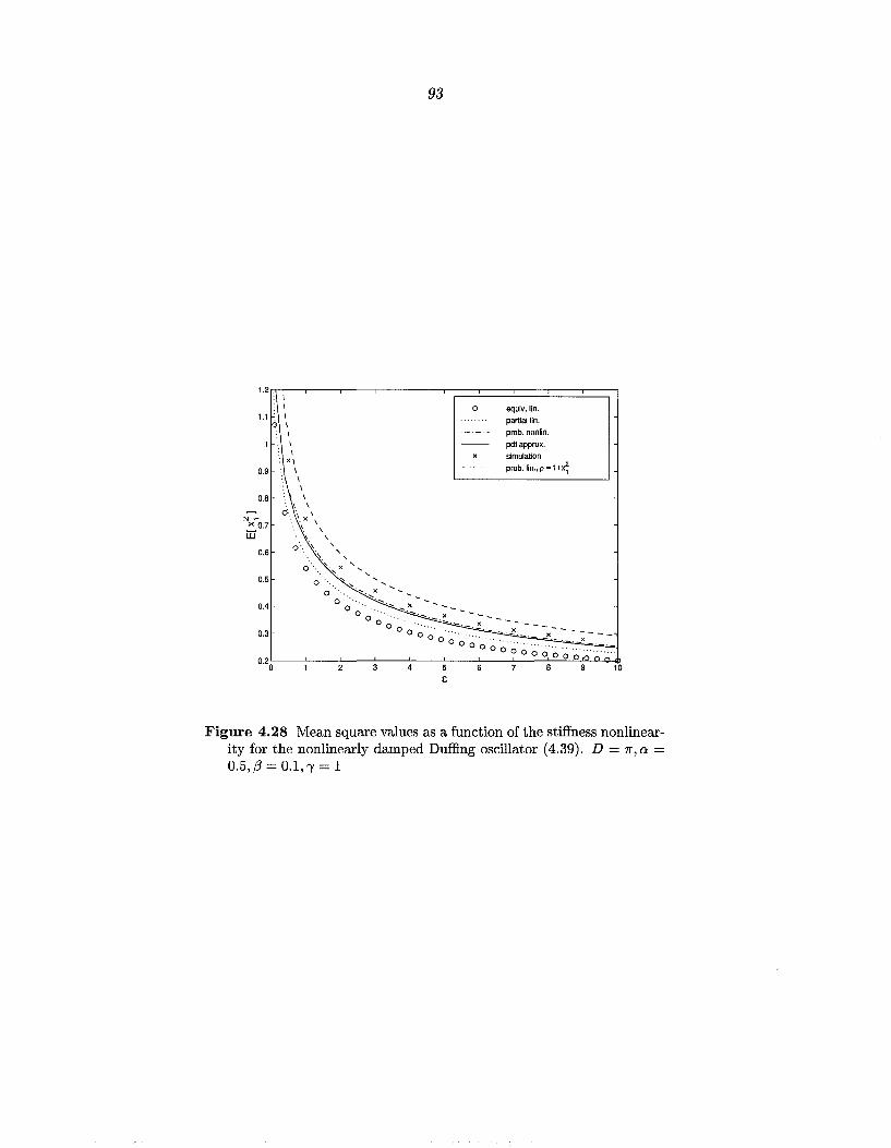
93

1.21J· -;----r-----.-----,---.--,--;::::::::::c::===c::==::::::=::!::::~

1.1 G I

"~ X 0.7 ti1

0.6

0.5 0

0.4

0.3

' ' ' ~-:-.._x ''

0 0

"· ' X ·~.

000 Oo

0 equiv.lin. partial/in. prob. nonlin.

pdf approx. simulation prob. lin., p = 1 +x~

0 0 0 0 0 ~ 0 ~~0;)~::~:·:~~·~~-:~.=~.; 0·2o'-----'----'-2 __ _.3 ___ 4'------'-5 ---'-6---'7 __ ..:.8'-"--"--'"-9J<LCL.o;)-14JO

E

Figure 4.28 Mean square values as a function of the stiffness nonlinear­ity for the nonlinearly damped Duffi.ng oscillator (4.39). D = 1r,a = 0.5, {3 = 0.1, 'Y = 1

94

Figure 4.29 Mean square values as a function of the damping nonlinear­ity for the nonlinearly damped Duffing oscillator (4.39). D = 1r,{3 = O.l,E = l,'"'f = 1

0.

0.12

0.1

~C\().oa .....

X cro.os

95

-2

2

1.5

0.5

XC\l 0

-0.5

-1

-1.5

-2

Figure 4.30 Stationary probability density function PF obtained by the directly approximating the Fokker-Planck equation for the nonlinearly damped Duffing oscillator. a = 0.5, (3 = 0.1, 'Y = 1, E = 1

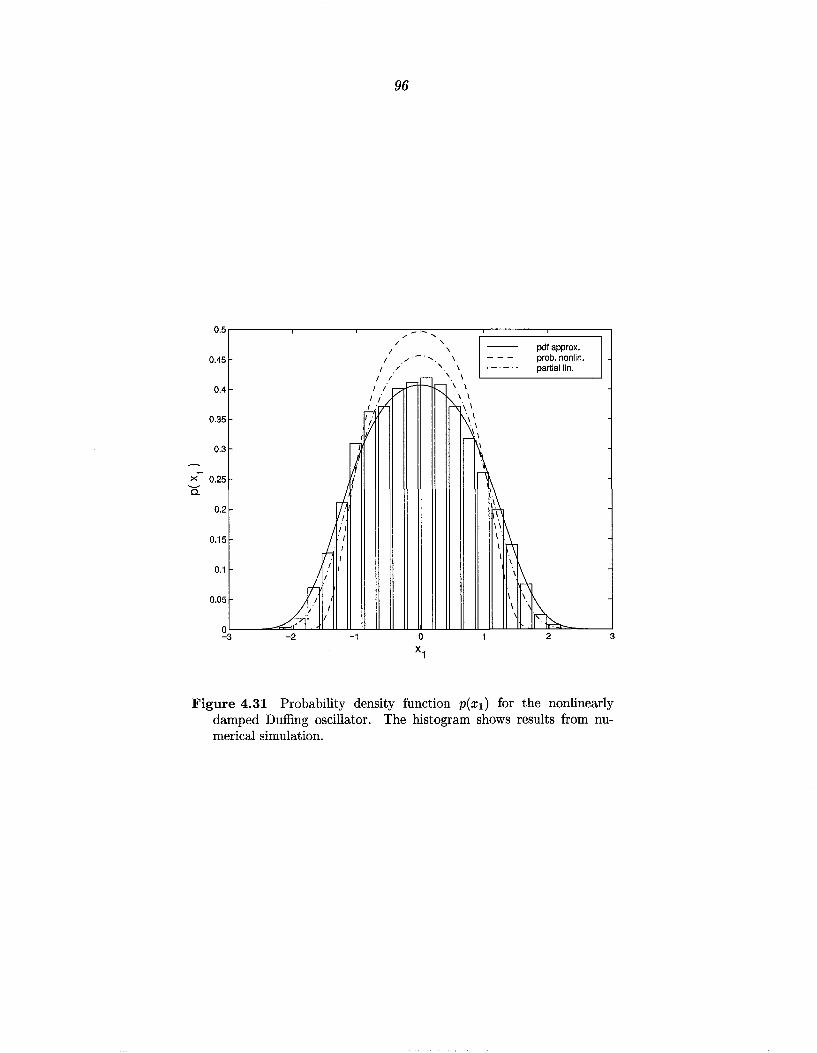
0.5

0.45

0.4

0.35

0.3

><~ 0.25 a:

0.2

0.15

0.1

0.05

0 -3 -2 -1

96

-- .... / '

I \ I .r - . ....._ \

\':\ I 1r" I.

\~

pdf approx. prob. nonlin. partial lin.

\ \ 1\ 'I~

2 3

Figure 4.31 Probability density function p(x1 ) for the nonlinearly damped Duffing oscillator. The histogram shows results from nu­merical simulation.

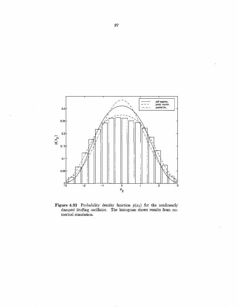
C\1 X

!5:

0.3

0.25

0.2

0.15

0.1

I ,.,.--0.05

~v 0 -3

r5' I I w I I

I I I.

r-f"i

IV

-2 -1

97

/ ... -- pdf approx . /

' / --- prob. nonlin. \ ·-·-·- partial lin. I \

I ---- \ .~·~--- -............ , I"

~ ""·~ \ ~

'~ \ \

\ r-\

~ \ ~ \

1\ \ ~

2 3

Figure 4.32 Probability density function p(x2 ) for the nonlinearly damped Duffing oscillator. The histogram shows results from nu­merical simulation.

98

computing outcrossing rates. The outcrossing rates for the safe set

{ S = X E IR2 : X1 E ( -b, b)}

computed by the various methods are shown in Figure 4.33. Also shown are esti­

mates obtained by using the method of probabilistic linearization and minimizing

the weighted £ 2 norm of the Fokker-Planck equation error, where the weighting

function is chosen as in the earlier sections on outcrossing rate estimation to place

emphasis near x1 = ±b. The value of the variance parameter in the weighting

function is a-~ = £ .

.......... -:-.. - ..

X

1.5

pdf approx. prob. lin., wtd. norm equiv.lin. prob. nonlin. simulation

2 Threshold level, b

' '

2.5

' ' ' ' ' ' ' \

\ \

\

\ I

I I

I I

3

Figure 4.33 Outcrossing rate estimation for the nonlinearly damped Duffing oscillator. D = 1r, a = 0.5, (3 = 0.1, 'Y = 1, t: = 0.5

As in example 3, it is observed that the outcrossing rates predicted by prob­

abilistic nonlinearization are far less than those predicted by the other methods.

Also, notice that the best agreement with the simulation results is obtained by the

99

direct approximation of the probability density function. For this example, the out­

crossing rate for probabilistic nonlinearization decays as e-Cib8

while for the direct

probability density function approximation, pp, the outcrossing rate goes as e-c2b4

,

and as e-c3 b2

for the method of equivalent linearization.

4.5 Equivalent and Partial Linearization Revisited

Although the methods of equivalent and partial linearization were developed by

approximating the stochastic differential equation, it is interesting to see how these

methods could be derived from the Fokker-Planck equation and how they compare

with the proposed methods.

Consider the single degree-of-freedom oscillator

(4.55)

with the associated stationary Fokker-Planck equation

4.5.1 Equivalent Linearization

In the method of equivalent linearization, (4.55) is replaced by a linear system. The

corresponding probability density function for the system response is given by

Substituting Plin into the Fokker-Planck equation (4.56) gives

100

Minimizing the mean-square value of each term in parenthesis, i.e. solving

gives

which are the variances given by the method of equivalent linearization.

4.5.2 Partial Linearization

In the method of partial linearization, the nonlinear system ( 4.55) is replaced by a

linearly damped system

=( x2 )dt+( 0 )dw(t)

-f3eqX2- g(xl) v'2J5

which has the corresponding stationary probability density function

( 1(3 ) _ (-f3eqG(xi) _ f3eqX~) Ppl x eq - c exp D 2D

where G(x1 ) = J;1 g(e) de and cis a normalization constant.

Notice that

so that error in the stationary Fokker-Planck equation (4.56) reduces to

101

Minimizing the mean square value of the term in parenthesis with respect to f3eq

gives

which is the partial linearization criterion (3.20).

4.6 Summary

Three new methods have been presented for analyzing nonlinear dynamical systems

under additive stochastic excitation and several examples were presented illustrating

the accuracy of the methods. The first method presented, probabilistic linearization,

finds the Gaussian probability density function that minimizes the Fokker-Planck

equation error. Since the probability density function for the response of linear

systems is Gaussian, this method is expected to work well for systems with small

nonlinearities. In addition, it was shown that simple weighting functions can be used

to improve the estimates for mean square values and outcrossing rates. The second

method presented, probabilistic nonlinearization, finds a non-Gaussian approxima­

tion to the stationary probability density function for the response of the system.

For the example considered, this method gave a smaller error in the Fokker-Planck

equation error than probabilistic linearization and provided better estimates to the

mean square values for the response, but provided poor estimates for outcrossing

rates. In the third method presented, a different set of approximate non-Gaussian

probability density functions than those chosen by the method of probabilistic non­

linearization is used. For the examples considered, this method provided good

estimates to both mean square values and outcrossing rates, as well as having the

smallest error in the Fokker-Planck equation.

102

Chapter 5

Modeling Uncertainty

In previous chapters, methods for predicting the response of dynamical systems

subjected to uncertain excitation were presented. No uncertainty in the modeling

of the system was considered. In this chapter, modeling uncertainties will also be

included in the analysis.

The response of dynamical systems is often modeled by a system of ordinary

or partial differential equations. The equations are usually obtained from balance

laws, experimental observations, or some combination of the two. One source of

modeling uncertainty, prediction-error uncertainty, is present in any model, as no

mathematical model can fully describe the behavior of a physical system. A sec­

ond source of modeling uncertainty is parameter uncertainty. The models typically

contain a number of parameters and the values of the parameters that will give the

best fit between the response of the model and the physical system are uncertain.

The uncertainty in the parameters will be modeled probabilistically, and typ­

ical problems arising when including modeling uncertainty in the analysis involve

computing integrals of the form

(5.1) I= fe j(O)p(O) dO

where f ( 0) and p( 0) are sufficiently smooth, 8 C !Rn, f ( 0) > 0 for all 0 E 8, and

p( 0) is a probability density function. Two applications in which integrals of the

form ( 5.1) arise are

103

1. Computing the statistical quantities of interest for an uncertain dynamical

system under stochastic excitation. For example, computing the expected

out crossing rate for an uncertain dynamical system is done by choosing f ( 0) =

v(O) where v(O) represents the conditional outcrossing rate for the system given

the parameters 0.

2. Classical reliability integrals. Classical reliability integrals arise in a number of

applications; see Madsen et al. (1986) for a number of examples and references.

For these integrals, regions of the parameter space (the safe set) are determined

to give acceptable performance, while other regions (the unsafe, or failure,

set) give unacceptable performance. In this case, it is desired to determine

the probability of acceptable [unacceptable] performance. This is done by

choosing f(O) = 1 and 8 to be the safe [failure] set.

In almost all cases where these integrals arise, the integrals cannot be evaluated

analytically. Numerical integration can be done to evaluate the integrals, but this

is often computationally expensive for a small number of uncertain parameters, and

usually prohibitive in more than six or seven dimensions. Another approach is to

use Monte Carlo-type methods. Although these methods typically require a large

number of samples, the computational cost is virtually independent of the number

of uncertain parameters, enabling the methods to be used for large problems. These

methods become especially expensive if the function f ( 0) is costly to evaluate or

when trying to determine failure probabilities, where the actual value of the integral

is often very low, in which case an exceptionally large number of samples is often

required.

Another method for approximating integrals of the form (5.1) is to obtain an

asymptotic expansion for the integral. This approach has recently been used to

determine the outcrossing rates, reliability, and moments for uncertain linear dy­

namical systems (Papadimitriou et al. 1995, 1997; May 1997) and has shown to give

accurate results in a number of examples. The general theory for the asymptotic

expansions is given in the next section and the expansion is applied to determine

moments and outcrossing rates for nonlinear dynamical systems in section 5.2 and

104

to evaluate classical reliability integrals in sections 5.4.3 and 5.5.

5.1 Asymptotic Approximation For A Class Of Proba­

bility Integrals

Consider the general class of multidimensional integrals of the form ( 5.1). Papadim­

itriou, Beck, and Katafygiotis (1995, 1997) have derived an asymptotic approxima­

tion based on an expansion of the logarithm of the integrand about the point that

corresponds to the maximum of the integrand. The idea is to rewrite the integral

(5.1) as

I= fe exp (P(O)) dO

where

P(O) = lnj(O) + lnp(O).

Note that since exp(·) is a monotonic function, the maxima of P(O) are the same as

the maxima of the integrand. Consider first the case for which P(O) has only one

maximum, (:}*, located in the interior of 8. Expanding P(O) in a Taylor series about

(:}* and using VP(O*) = 0 gives

P(O) = P(O*) - (0- O*)T L(O*)(O- (:}*) + e(O)

where L(O) = -VVP(O) and e(O) = 0 (IIO- 0*11 3). Substituting the series expansion

into the integral (5.1) gives

I exp(P(O*)) fe exp ( -({:}- O*f L(O*)((:}- (:}*)) exp(e(O)) d(:}

f ( O*)p( 0*) fe exp ( -( (:} - O*)T L( (:}*)( (:} - (:}*)) exp( e( 0)) dO.

105

Applying Laplace's method of asymptotic expansion (Bleistein and Handelsman

1986) to the above integral yields

(5.2) I()* (27r)n/2 j(()*)p(()*)

( ) "' Jdet L({)*) ·

Letting A be the minimum eigenvalue of L(()*), it can be shown that the approx­

imation becomes asymptotically correct as A -+ oo. Thus, it is expected that the

accuracy of the approximation increases as A increases, which corresponds to the

integrand becoming more "peaked" around the maximum.

If there are a finite number of global maxima of the integrand in e, the above

procedure can still be applied by summing the contributions from each maximum.

Letting the maxima be e;, i = 1, ... k, the approximation for the integral is given

by

k

I= LJ(ei). i=l

A method which can be used to locate the multiple maxima has been developed by

Yang and Beck (1998).

5.2 Moments and Outcrossing Rates for Uncertain Non­

linear Dynamical Systems

To determine the moments and outcrossing rates for nonlinear dynamical systems

with uncertain parameters, it is first necessary to be able to determine the con­

ditional moments and outcrossing rates for given parameters. The values can be

determined exactly only for certain nonlinear systems, as discussed in chapter 3,

but they can be determined approximately by the methods of chapter 4 for other

nonlinear systems.

Letting () E IRm be the uncertain parameters with probability density function

p(()), E[xil()] be the conditional moments and v(()) the conditional outcrossing rate,

106

the moments and outcrossing rate for the uncertain system are

(5.3a) E[xf] = { E[xf!O]p(O) dO }fRm

(5.3b) v= { v(O)p(O)dO. }fRm

5.2.1 Example 1: Uncertain Duffing Oscillator

In this section, the accuracy of the asymptotic approximation for computing the

moments and outcrossing rates for the uncertain, linearly damped Duffing oscillator

will be investigated. The Duffing oscillator considered is

(5.4)

where (,wn,E, and Dare all uncertain and n(t) is zero-mean, Gaussian white noise

with E[n(t)n(t+r)] = o(r). The uncertain variables are taken to be independently,

lognormally distributed. The lognormal probability density function with mean

parameter me and variance parameter ao is given by

(5.5) (e)- 1 ( (ln0-mo)2) forall0>0. Po - '2= ll exp - 2 2 VL.1fUa() a()

The mean parameters for the probability density functions are chosen as

mwn= ln 1

mv = ln 0.75

me.= ln 0.5

me= ln 0.25.

The mean values for the uncertain variables vary slightly with the variance param­

eter for the probability density function, but using the above parameters gives

E[wn]:::::: 1

E[D] :::::::0.75

E[(]::::::: 0.5

E[t]::::::: 0.25.

The value of the variance parameter, a, in the lognormal probability density function

is approximately the coefficient of variation for the uncertain variable. A common

107

value of (} will be taken for this parameter and the dependence of the results on (}

will be investigated.

The stationary probability density function for the Duffing oscillator (5.4) given

the parameters (} is

where a((, Wn, E, D) is the normalization constant for the probability density func­

tion. The conditional moments and outcrossing rates can easily be computed from

the probability density function and the moments and outcrossing rate for the un­

certain system are given by the integrals (5.3a,5.3b).

The effect of parameter uncertainty on both mean square values and expected

outcrossing rates for the Duffing oscillator is illustrated in Tables 5.1-5.5 and Fig­

ure 5.1. In order to investigate the sensitivity of the results to the parameters,

results are presented for cases when only one or two of the variables are considered

to be uncertain, as well as for cases when all of the variables are uncertain. When

only some of the variables are considered uncertain, the variables which are not

considered to be uncertain are set to their mean values.

Results obtained by the asymptotic approximation are compared with those ob­

tained by evaluating the integrals numerically. For one or two uncertain parameters,

the numerical integration is done directly. For more than two uncertain variables, di­

rect numerical integration becomes too computationally expensive, and the method

of importance sampling (Schueller and Stix 1987; Bucher 1988) is used to compute

the integrals. Importance sampling is a Monte Carlo-type method in which most of

the samples are generated in the region where the integrand is largest. The weight­

ing functions used in the importance sampling computations are the same as those

used in Papadimitriou et al. (1995).

The results illustrate several points. First, the asymptotic approximation pro­

vides good estimates for the integrals even when there is large uncertainty in the

parameters. Additionally, it is observed that the outcrossing rate, and hence the

108

probability of failure, is much more sensitive to parametric uncertainty than the

mean square values are. Even for coefficients of variation of 10% on the parameters,

the expected outcrossing rate is more than an order of magnitude greater than the

outcrossing rate obtained by using the mean values of the parameters. It is also

observed that both the mean square values and the outcrossing rates are most sen­

sitive to uncertainty in the natural frequency and least sensitive to uncertainty in

the nonlinear stiffness term, E.

Uncertain variable ( D E Wn Numerical integration 0.54 0.52 0.53 0.57

Asymptotic approximation 0.53 0.51 0.52 0.56

Table 5.1 Mean square values, E[x2], for the linearly damped Duffing oscillator with one uncertain variable with variance parameter a = 0.2. The variables which are not considered as uncertain are set to their mean values. The mean square value with all of the variables set to their mean values, E[x2 IB], is 0.53.

Uncertain variables E,( (,D E,Wn Wn,( Wn,D Numerical integration 0.54 0.54 0.57 0.58 0.56

Asymptotic approximation 0.52 0.52 0.55 0.56 0.54

Table 5.2 Mean square values, E[x2], for the linearly damped Duffing oscillator with two uncertain variables with variance parameter a = 0.2. The variables which are not considered as uncertain are set to their mean values. The mean square value with all of the variables set to their mean values, E[x2 !BJ, is 0.53.

Variance parameter, a 0.05 0.10 0.15 0.20 Importance sampling 0.55 0.56 0.57 0.58

Asymptotic approximation 0.55 0.55 0.54 0.54

Table 5.3 Mean square values, E[x2], for the linearly damped Duffing oscillator when all of the variables are uncertain with variance param­eter a.

109

105 r-----.------.-----,,-----,------,-----,------.-----.

10" v

v(e)

10' asympt. approx.

o import. samp.

100L-----~----~------~----~----~----~------~----~ 0 0.05 0.1 0.15 0.2

cr 0.25 0.3 0.35 0.4

Figure 5.1 Expected outcrossing rates for the Duffing oscillator when all of the variables are uncertain with variance parameter CT. The plot shows the ratio of the expected outcrossing rate v obtained by eval­uating the integral (5.3b) to the outcrossing rate obtained by setting all of the parameters to their mean values, v(iJ).

110

Uncertain variable ( D E Wn Numerical integration 7.10 X 10 -6 4.88 X 10 -6 1.34 X 10 -o 6.46 X 10 -t>

Asymptotic approximation 7.02 X 10 -o 4.80 X 10-o 1.21 x 10-6 6.48 x 10-5

Table 5.4 Outcrossing rates for the linearly damped Duffing oscillator with one uncertain variable with variance parameter a = 0.2. The variables which are not considered as uncertain are set to their mean values. The outcrossing rate with all of the parameters set to their mean values is v(O) = 6.07 x 10-7 .

Uncertain variables E,( (,D E,Wn Wn,( Wn,D Num. int. 1.08 X 10 -t> 2.14 X 10 -t> 9.42 X 10 -t> 1.40 X 10 -4 1.12 X 10 -4

Asymptotic 1.06 x 10-5 2.05 x 10-5 9.35 X 10 -5 1.40 X 10 -4 1.09 x 10-4

Table 5.5 Outcrossing rates for the linearly damped Duffing oscillator with two uncertain variables with variance parameter a = 0.2. The variables which are not considered as uncertain are set to their mean values. The outcrossing rate with all of the parameters set to their mean values is v(iJ) = 6.07 x 10-7 •

5.2.2 Example 2: Rolling Ship with Uncertain Parameters

The second example is the rolling ship, which was considered earlier is section 4.4.2

x + 2(wnx + a!x!x + w~x + Ex3 = V2i5 n(t).

The uncertain parameters for the system are taken to be(}= ((,a,wn,E,D).

In this case, the stationary Fokker-Planck equation cannot be solved exactly

and the stationary probability density function must be determined approximately

to determine the conditional moments and outcrossing rates. It was seen in the

previous example that the outcrossing rates are much more sensitive to uncertainty

in the parameters than the mean square values are, and for this example, only

outcrossing rates will be considered. It was shown in chapter 4 that the outcrossing

rates for nonlinear systems can be approximated either by using a weighted norm

in the method of probabilistic linearization or by using the direct approximation of

the probability density function with a non-Gaussian probability density function,

as in section 4.4. For this example, a non-Gaussian probability density function is

111

chosen as in 4.4.2. The approximate probability density function chosen is

where ¢ is the parameter of the approximate probability density function which was

called in 0 in section 4.4 and a(O) is a normalization constant. Equation {4.48) gives

The expected values in the above equation can be computed analytically, but the

resulting expressions are rather complicated and are not presented here. The ex­

pected outcrossing rate for the threshold x = b and the system parameters 0 is given

by

{5.7) v(O) = fooo xp(b, xi¢(0), 0) dx.

The above integral can also be evaluated analytically, again yielding a rather com­

plicated expression. Accounting for the uncertainty, the expected outcrossing rate

is

v = { v( O)p( 0) dO }IRs

where p(O) is the probability density function for the uncertain variables. The

variables are assumed to be independently, lognormally distributed with parameters

mwn = ln 21!"

ffi( = ln 0.05

ma ln 0.5

mE = ln 0.25

ffiD ln 100.

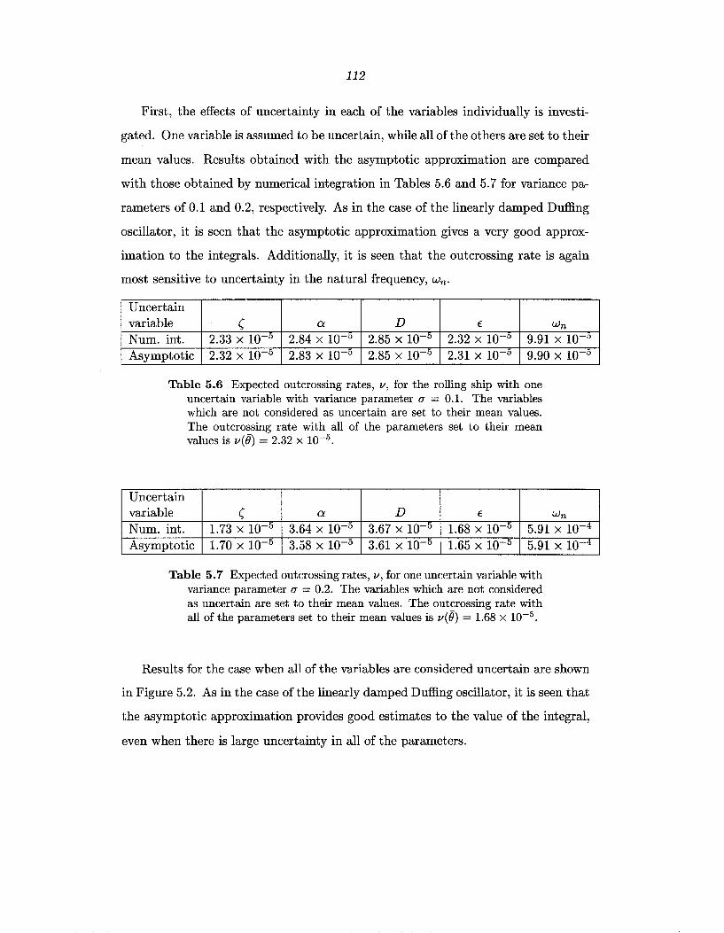
112

First, the effects of uncertainty in each of the variables individually is investi­

gated. One variable is assumed to be uncertain, while all of the others are set to their

mean values. Results obtained with the asymptotic approximation are compared

with those obtained by numerical integration in Tables 5.6 and 5. 7 for variance pa­

rameters of 0.1 and 0.2, respectively. As in the case of the linearly damped Duffing

oscillator, it is seen that the asymptotic approximation gives a very good approx­

imation to the integrals. Additionally, it is seen that the outcrossing rate is again

most sensitive to uncertainty in the natural frequency, Wn.

Uncertain variable ( a D € Wn

Num. int. 2.33 x w-5 2.84 x w-5 2.85 x w-5 2.32 x w-5 9.91 x w-5

Asymptotic 2.32 X 10 -o 2.83 X 10 -o 2.85 X 10 -o 2.31 X 10 -o 9.90 X 10 -o

Table 5.6 Expected outcrossing rates, v, for the rolling ship with one uncertain variable with variance parameter u = 0.1. The variables which are not considered as uncertain are set to their mean values. The outcrossing rate with all of the parameters set to their mean values is v( 0) = 2.32 X 10-5•

Uncertain variable ( a D € Wn

Num. int. 1.73 X 10 -b 3.64 X 10 -b 3.67 X 10 -b 1.68 X 10 -5 5.91 x w-4

Asymptotic 1.70 X 10 -5 3.58 X 10 -5 3.61 X 10 -5 1.65 X 10 -o 5.91 X 10 -'±

Table 5. 7 Expected outcrossing rates, v, for one uncertain variable with variance parameter u = 0.2. The variables which are not considered as uncertain are set to their mean values. The outcrossing rate with all of the parameters set to their mean values is v( 0) = 1.68 x w-5 •

Results for the case when all of the variables are considered uncertain are shown

in Figure 5.2. As in the case of the linearly damped Duffing oscillator, it is seen that

the asymptotic approximation provides good estimates to the value of the integral,

even when there is large uncertainty in all of the parameters.

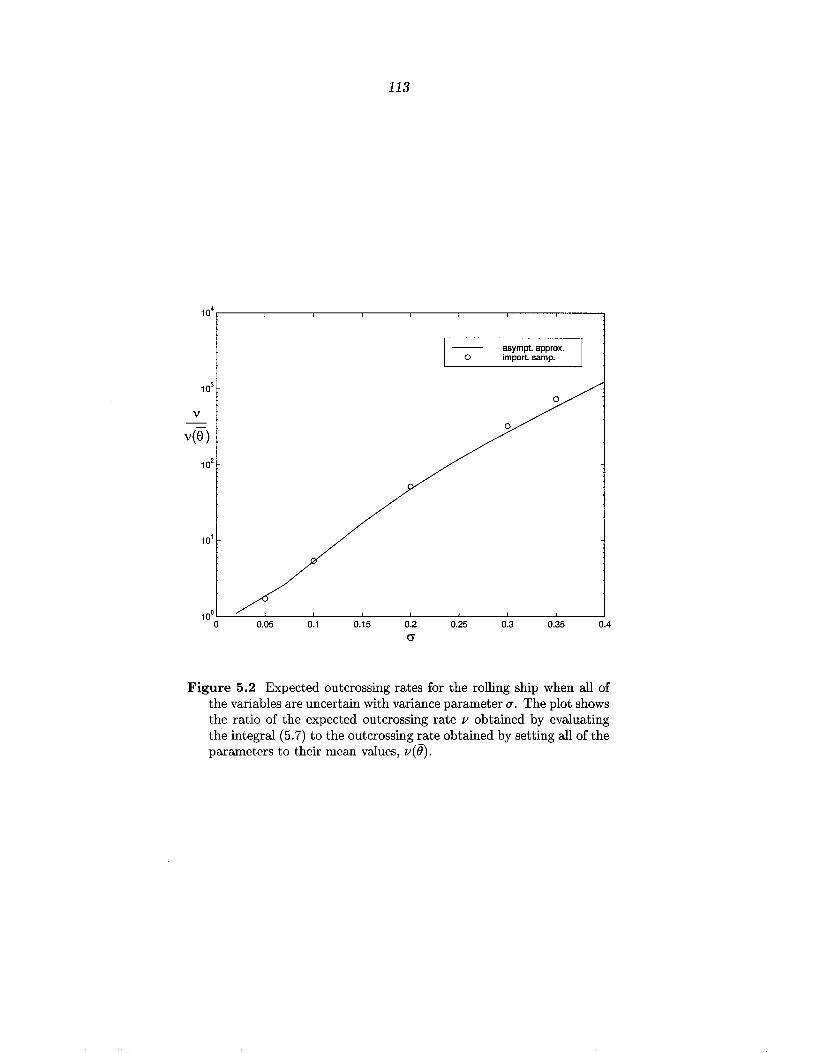
113

104 r-----.------.-----.------.------.-----.------~----~

asympt. approx. o import. samp.

0

v 0

v(e)

10'

10°~----~----~----~------~----~----~------~----~ 0 0.05 0.1 0.15 0.2

(j

0.25 0.3 0.35 0.4

Figure 5.2 Expected outcrossing rates for the rolling ship when all of the variables are uncertain with variance parameter a. The plot shows the ratio of the expected outcrossing rate v obtained by evaluating the integral (5.7) to the outcrossing rate obtained by setting all of the parameters to their mean values, v(iJ).

114

5.3 Classical Reliability Integrals

In classical reliability integrals, the parameter space is divided into two regions,

the safe region, S and the unsafe, or failure, region, :F. If the parameter values

are in the safe region, the system will have acceptable performance, whereas for

parameter values in the unsafe region, the system performance will be unacceptable.

The probability density function for the parameters is given by p( 0) and the goal is

to assess the probability of failure, which can be obtained from the integral

(5.8) pf = L p(O) dO.

Integrals of the form (5.8) cannot typically be evaluated analytically and nu­

merical evaluation becomes computationally prohibitive as the number of unknown

parameters increases. In order to evaluate these integrals, some approximate tech­

niques have been developed. The FORM and SORM methods are reviewed in the

next section.

5.4 FORM and SORM Approaches

Two of the most common methods for approximating reliability integrals are the first

and second order reliability methods (FORM and SORM, respectively). The first

step in either of the methods is to make a transformation of coordinates from the

original parameters 0 to new variables x so that the new variables are independently,

normally distributed, i.e.,

1 ( 1 2) p(x) = <P(x) = (21r)n/2 exp -211xll .

One such transformation which is applicable to any original distribution p( 0) is the

Rosenblatt transformation (Rosenblatt 1952), as discussed in Madsen et al. (1986).

The second step in the FORM and SORM methods is to approximate the bound­

ary between the safe and unsafe regions by either a first or second order surface.

First, consider the case where there is a single surface separating the safe and unsafe

115

regions in the new variables x. This surface, termed the failure surface, is typically

given in the implicit form g(x) = 0 and the safe and unsafe sets are the regions

S {x E IRn : g(x) < 0}

F {x E IRn : g(x) > 0}.

The probability of failure integral becomes

Pf = { ¢(x) dx. }g(x)>O

This integral can be evaluated analytically only when the failure surface is a hyper­

plane. In the FORM and SORM methods, the failure surface is approximated by

either a first or second order surface in the vicinity of the point on g(x) = 0 with

minimal distance to the origin. The idea behind these approximations is that ¢( x)

decays rapidly as llxll increases, so the major contributions to the integral come

from the regions in F closest to the origin. The point on the failure surface closest

to the origin in the transformed x-space is called the design point and the distance

from this point to the origin is often denoted by j3.

If there is more than one surface separating the safe and unsafe regions, the

surface approximations are made at the design point on each surface, and the integral

can be approximated by summing the contributions from each surface, provided that

the contribution from the overlapping failure domains is insignificant. A more formal

study of system reliability issues can be found in the books by Madsen et al. (1986)

and Thoft-Christensen and Murotsu (1986).

5.4.1 FORM

In first-order reliability methods, the failure surface is approximated by a hyperplane

tangent to the surface at the point on the surface closest to the origin, as illustrated

in Figure 5.3. The approximating hyperplane can be written in the form

9Jorm(x) = (x, n)- f3 = 0

116

Failure surface, fi.~ = 0 F

FORM approximation , to failure surface '

s

------------~-------------X1

Figure 5.3 FORM approximation to the failure surface

where n is the unit normal to the hyperplane. With this approximation to the failure

surface, the integral can be evaluated analytically (Madsen et al. 1986), giving

(5.9) r ¢(x)dx = <I>(-,6) }9form(x)>O

where <I>(·) is the standard normal cumulative distribution function. This is the

value used by the FORM approach to obtain estimates of the failure probability,

i.e.,

Pf ~ <I>( -,6).

5.4.2 SORM

In the second-order reliability methods, the curvature of the failure surface at the

design point is also accounted for. In this case, a second-order surface is used to

approximate the failure surface in the vicinity of the design point, as shown in

Figure 5.4.

After a rotation of coordinates, the paraboloid approximation to the failure

Failure surface, [f._~ = 0

117

I I I I I I I

F

SORM approximation to failun;' surface

Figure 5.4 SORM approximation to the failure surface

surface can be written in the form

(5.10) n-1 1~ 2

Ysorm(x) = Xn- 2 ~ aiXi - f3 = 0 i=l

where the ai's are the principal surface curvatures at the design point and the Xn axis

is along the line through the origin and the design point. An alternative procedure

for obtaining a second order approximation based on a point-fitting method rather

than curvature fitting has been given by Der Kiureghian et al. (1987). In either

case, the probability of failure is then approximated by the following integral

(5.11) Pt ~ { <f;(x) dx. } 9sorm(x)>O

Unlike the FORM case, the above integral cannot be evaluated analytically, and a

further approximation is required. A few different asymptotic approximations have

been previously developed for approximating integrals of the form (5.11) (Tvedt

1983; Breitung 1984; Ki::iyliioglu and Nielsen 1994). In Breitung's approximation,

118

the asymptotic expansion obtained is

(5.12)

This approximation is valid for f3ai > -1 for all i and becomes asymptotically exact

as (3 --+ oo. Tvedt's approximation consists of a sum of three terms, the first of

which is Breitung's formula (5.12) and the second and third terms are somewhat

more complicated expressions. Koyliioglu and Nielsen used asymptotic expansions

of the cumulative distribution function to obtain a number of different approxima­

tions, depending on the signs of the surface curvatures and the order of derivatives

which were matched in the expansion. In the next section, the asymptotic expan­

sion discussed in section 5.1 is used to give a simple derivation for an alternative

asymptotic expansion to SORM integrals.

5.4.3 A New Asymptotic Expansion for SORM Integrals

The asymptotic method described in section 5.1, provides a very simple means for

obtaining an asymptotic expansion for SORM integrals. The expansion differs from

Breitung's formula, although the two formulas become asymptotically equivalent as

(3--+ 00.

The SORM integral is written as

where F = {x E !Rn : 9sorm(x) > 0}. The approximation described in section 5.1

is not directly applicable to this integral, since the point maximizing the integrand

(the design point) is on the boundary of F. Recall from (5.10) that the failure

surface is given by Xn = (3 + ~ I:~;/ aixt. In order to simplify the notation in

the following, let y = (x1, ... Xn-I), m = n- 1, and order the curvatures so that

119

a1 ::::; a2 ::::; ... ::::; am. With this notation, the integral can be rewritten as

(5.13)

J.m ( l:! L'z:;, a;yf <P(xn) dxn) ,P(y) dy

J.m <1> ( -fJ - ~ ~ a;yi) ,P(y) dy.

The integral (5.13) is over all of !Rm, ensuring the maxima of the integrand will

be in the interior and that the asymptotic expansion (5.2) can be applied. For

most cases of engineering interest, this is especially easy, as given by the following

theorem.

Theorem 5.1 Applying the asymptotic expansion (5.2) to the integral in (5.13),

and considering separately the three cases of system parameters which are distin­

guished by the number of maxima of the integrand, gives the following:

Case 1: If a1 :~ =~~ > -1,

(5.14)

(5.15)

p <P( -,B) f rv nm v <P( -{3) .

i=1 1 + ai ~( -!3)

( ( ~)) <P ( -.e- a1 'YI /2) exp ( -')'r /2)

Pf "' 2 1 - <P -')'1 y hn Jdet L(y*)

where hn = ,Ba1 + ahr /2 + 1, ')'1 is the unique positive solution of

and

(5.16)

1 + a1 ¢( -,8- anU2) = 0 <P( -,8- anU2)

det L(y*) = 'YI hn IT (1 -:i) . i=2 1

120

(5.17)

where h = f3a1 + a 1 "(2 /2 + 1, 'Y is the unique positive solution of

and

(5.18)

Proof:

The proof of case 1 is presented here and the proofs for cases 2 and 3 are given

in appendix B. The first step in the asymptotic method is to find the point(s)

maximizing the integrand. In this case, there is a unique maximum, as given by the

following lemma, which is proved in appendix B.

Lemma 5.1 If a1 :~=~~ > -1, then the integrand in (5.13) possesses a unzque

maximum, y* = 0.

The next step is to compute the determinant of the Hessian matrix at y*. Letting

f(y) = ln<I>(-/3- ~ L~=l aky~) + ln¢(y) and L(y) = -'\1'\lf(y), as in section 5.1,

the determinant of L(y*) can be easily evaluated from the following lemma, which

is also proved in appendix B.

Lemma 5.2 Ifal:~=~~ > -1, then the determinant of the Hessian matrix L(y*) is

given by

* lim ( ¢(-/3)) det L(y ) = i=l 1 + ai <I>( -{3) ·

121

Thus, from equation (5.2), the asymptotic expansion is given by

(5.19) p * (27r)m/2 J(y*)cp(y*)

J(Y ) "' yfdet L(y*)

where f(y) = ip( -(3- ~ 2:'.:~=l aky~). Using y* = 0, the following results are easily

obtained

f(y*) = ip(-(3)

cp(y*) (27r)-m/2.

Substituting the above quantities into (5.19) proves case 1 of the theorem. •

Note that, except for the correction factor of (1 - ip( --y1hn)) discussed in ap­

pendix B, equation (5.17) reduces to equation (5.15) in the special case of k = 1.

Also notice that as a2 ---+ a1 in equation (5.15), Pf becomes unbounded and for

a2 close to a1 the smaller of (5.15) and (5.17) with k = 2 should be used as the

approximation. Similarly, if a3 and a2 are close to a1, (5.17) can be used with k = 3,

and so on for more curvatures close to a1.

Some comments about the new asymptotic expansion

The formula (5.14) was obtained by a different approach based on a McLaurin series

expansion of the cumulative distribution function which was valid only for ai > 0

for all i by Koyliioglu and Nielsen (1994). Koyliioglu and Nielsen used a different

asymptotic expansion for cases when all of the ai < 0 and a third expansion in the

case of some ai > 0 and some ai < 0. Formula (5.14) also appeared in a derivation

of an importance sampling expression given by Hohenbichler and Rackwitz (1988).

The expansion developed for case 1 is valid as long as ai :~=~~ > -1. For large (3,

this is similar to the condition that aif3 > -1, since :t =~~ "' (3 as (3 ---+ oo. This

latter condition is usually satisfied in practice, since no point on the failure surface

can be inside a hypersphere of radius (3 if (3 is the shortest distance from the failure

surface to the origin. Thus, for concave failure surfaces, the magnitude of the surface

curvatures at the design point must be less than the curvature of the hypersphere of

122

radius {3, giving the condition aif3 > -1. However, for finite values of {3, there exists

a range of curvatures for which ai :~ =~~ < -1 but aif3 > -1. For these parameter

values, the expansions developed for cases 2 and 3 should be used.

Notice that the new formula given by (5.14) is very similar to Breitung's formula

(5.12). The only difference is that the terms (1 + aif3) in Breitung's formula become

replaced with 1 + ai :t =~~. Additionally, since :t =~~ "' f3 as f3 --t oo, it is seen that

the two formulas are asymptotically equivalent in the limit as f3 --too. However, for

finite values of {3, values obtained by the two approximations will differ. Numerical

comparisons of the two approaches are presented later in Tables 5.8-5.10.

It is of interest to compare the two approximations (5.12) and (5.14) for small

values of surface curvatures. In order to do this, consider the asymptotic approxi­

mations to the probability of failure as a function of the surface curvatures

In the case where all of the surface curvatures are zero, i.e., ai = 0 for all

i = 1, ... , m, both approximations give Pj(O) = <I>( -{3), which is the FORM ap­

proximation. Note that this is also the exact answer since with all ai = 0, the failure

surface is a hyperplane. In order to investigate the approximations for small cur­

vatures, consider the rate of change of Pj with respect to the curvatures, ~~f la=O· The exact value can be computed from

a:, (J.m g; ( -~- ~ t, a,y~) ¢(y) dy) a=O

l y~ _ __!_¢( -(3)¢(y) dy

IRm 2

1 i 2 --¢( -{3) Yi ¢(y) dy 2 IRm

¢( -{3) 2

123

For Breitung's approximation, the derivatives are computed as

whereas for the new approximation,

j3if!(- !3) 2

Notice that the new approximation provides the correct derivative, and thus for

small curvatures, the error in Pt(a) is of order ar, while the error in Breitung's

approximation is of the order lail·

Numerical Results

The following tables compare results obtained by the different approximations for

various values of j3 and surface curvatures. The formulas obtained by the new

approach, Breitung's approximation, and Koyliioglu and Nielsen's one term ap­

proximation are all very simple. The results obtained by the new approximation

are often more accurate than those obtained from these approximations. Tvedt's

approximation and Koyliioglu and Nielsen's three term approximation tend to give

more accurate results than the new approximation, but the formulas for these ap­

proximations are also considerably more difficult. The exact values presented in

Tables 5.8, 5.9 and 5.11 were obtained by Koyliioglu and Nielsen (1994) using a

Gaussian quadrature numerical integration scheme and the values in Table 5.10

were obtained using numerical integration in Mathematica.

All of the tables are for the case when n = 3. Table 5.8 is for the case when both

surface curvatures of the failure surface are positive. In this case, Koyliioglu and

Nielsen's one term approximation is the same as the formula for the new approx­

imation. In Table 5.9, both surface curvatures are negative, but small enough so

that ai:~:::~1 > -1. In Table 5.10, the case is considered when one of the negative

curvatures is large enough so that a1 :~ :::_~~ < -1 but small enough so that a1/3 > -1.

In this case, the formulas (B.8) and (B.10) are used for the new approximation. For

124

this case, the results from the new approximation are seen to be considerably better

than Breitung's approach, and of comparable or better accuracy to Koyliioglu and

Nielsen's approximation.

In Table 5.11, the results of the approximations are investigated when there is

a large negative surface curvature. For the cases considered, a1 ¢(-(3) / ifJ (-(3) < -1

and a1f3 < -1. While these cases are unlikely to occur in practice, it is interesting to

note that the new approximations provide much better (several orders of magnitude

for large (3) results than the other approximations in this case.

5.5 Application of Asymptotic Approximation in Orig­

inal Variables

As mentioned in section 5.4, the first step in either the FORM or SORM methods is

to make a transformation of variables from the original variables, (), to new variables

x, so that the new variables are independently normally distributed. While this can

always be done in principle through the Rosenblatt transformation, in many cases

the transformation cannot be performed analytically and must be done numerically,

which greatly increases the computational requirements. Additionally, by making

the transformation of variables, the sensitivity of results to changes in the original

parameters is not clear. For these reasons, it is desirable to be able to obtain

approximations in the original variables. Breitung (1989) has developed one such

formula, but the resulting expression is rather complicated. In this section, an

approximation is obtained by the same method used earlier for the transformed

variables, yielding a formula much simpler than Breitung's formula.

In the original variables, the probability of failure is given by

(5.20)

where p(O) is the probability density function for (). Letting m n- 1, '1/J

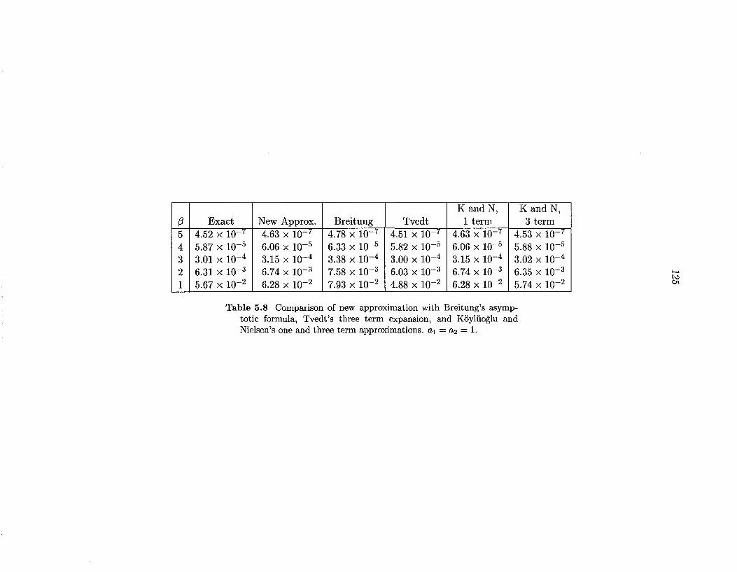
(3 5 4 3 2 1

K and N, K and N, I Exact New Approx. Brei tung Tvedt 1 term 3 term

4.52 X 10 I 4.63 X 10 I 4.78 X 10 7 4.51 X 10 -I 4.63 X 10 -7 4.53 X 10 I

5.87 x 10-5 6.06 x 10-5 6.33 x 10-5 5.82 x w-5 6.06 x w-5 5.88 x 10-5

3.01 x 10-4 3.15 x 10-4 3.38 x 10-4 3.oo x w-4 3.15 x w-4 3.02 x 10-4

6.31 x 10-3 6.74 x 10_3 7.58 x 10-3 6.03 x 10-3 6.74 x 10-3 6.35 x 10-3

5.67 x w-2 6.28 x 10-2 7.93 x 10-2 4.88 x 10-2 6.28 x w-2 5.74 x 10-2

Table 5.8 Comparison of new approximation with Breitung's asymp­totic formula, Tvedt's three term expansion, and Koyliioglu and Nielsen's one and three term approximations. a1 = a2 = 1.

f-.<

~

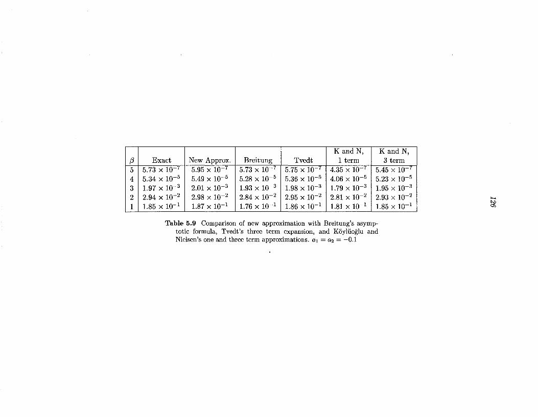
(3 5 4 3 2 1

K and N, K and N, Exact New Approx. Brei tung Tvedt 1 term 3 term

5.73 X 10 f 5.95 x w-'r 5.73 X 10 f 5.75 x w- 7 4.35 X 10 f 5.45 x w-7

5.34 x w-5 5.49 x w-5 5.28 x w-5 5.36 x w-5 4.06 x w-5 5.23 x w-5

1.97 x w-3 2.01 x w-3 1.93 x w-3 1.98 x w-3 1.79 x w-3 1.95 x w-3

2.94 x w-2 2.98 x w-2 2.84 x w-2 2.95 x w-2 2.81 x w-2 2.93 x w-2

1.85 x w-1 1.87 x w-1 1.76 x w-1 1.86 x w-1 1.81 x w-1 1.85 x w-1 -----------------

Table 5.9 Comparison of new approximation with Breitung's asymp­totic formula, Tvedt's three term expansion, and Koyliioglu and Nielsen's one and three term approximations. a1 = a2 = -0.1

f.-< ~ 0:,

K and N, K and N, a2 Exact New Approx. Brei tung Tvedt 1 term 3 term

-0.48 0.086 0.091 0.569 0.571 0.048 0.052 -0.10 0.055 0.075 0.127 n/a 0.038 0.039 0.50 0.035 0.047 0.080 n/a 0.023 0.036

Table 5.10 Comparison of SORM approximations when (3 = 2, a1 = -0.48. Tvedt's approximation gives complex numbers for the cases where "n/a" is given.

..... l;.,j

'"""

128

K and N, K and N, (3 Exact New Approx. 1 term 3 term 5 0.0020 0.0019 5.07 X 10-7 6.64 X 10-ti 4 0.0061 0.0059 5.18 X 10-5 0.0004 3 0.0200 0.0187 0.0020 0.0067 2 0.0693 0.0640 0.0063 0.0495 1 0.2185 0.2389 0.1789 0.2012

Table 5.11 Comparison of new approximation with Koyliioglu and Nielsen's one and three term approximations. a1 = -l,a2 = 1

(01, ... , Om) and a= On, the probability density function for 0 can be rewritten as

and the failure surface is g('ljJ, a) = 0. In terms of a and 7/J, the above integral can

be rewritten as

{ [ { p(ai1/J)da] P7f;(1/J)d'ljJ }'J?_m }g(7j;,o.)>O

(5.21) ~m J ( 1/J )P7f; ( 1/J )d'ljJ

where

(5.22) f('ljJ) = { Pa(ai1/J) da. }g(7j;,o.)>O

Applying the asymptotic approximation (5.2) to the integral (5.21) gives

(5.23)

where 7/J* is the point maximizing the integrand in (5.21), £(7/J) = lnf('ljJ) +lnp7f;(7/J)

and L('ljJ) = -\1\1£(7/J). If there is more than one maxima of the integrand, the prob­

ability of failure can be obtained by summing the contributions from each maximum.

A simpler formula than (5.23) can be obtained if the following two conditions

129

are satisfied

1. One of the parameters, say On, is independently distributed from the others.

In this situation, the probability density function for the parameters becomes

Po(O) = P'l/J('l/J)Pa(a), where a= On.

2. The failure surface g(O) = g('lj;, a) = 0 can be written as a = h('lj;), and the

safe region is the region a > h('lj;). Note that the implicit function theorem

guarantees that this can always be done locally provided that ~ f:. 0.

Under these conditions, the probability of failure becomes

Pf = { P'l/J ( '1/J) Pa (a) da d'lj; }g('l/J,a)>O

~ L (L:) Pa(a) da) P>!(¢) d,P

(5.24) km Pa(h('lj;))P'!jJ('l/J) d'lj;

where Pa(·) is the cumulative distribution function for a. Laplace's method of

asymptotic expansion can be applied to the integral (5.24). Letting '1/J* be the value

of 'lj; which maximizes the integrand (assuming there is only one maximum), the

asymptotic approximation is given by

(5.25) p (27r)mf2 Pa(h('lj;*)) P'!jJ('l/J*) f"' vfdetL('lj;*)

where L('lj;) = -\7\lf('l/;) and f('l/;) = lnPa(h('l/;)) + lnp'I/J('lj;). As usual, multiple

maxima can be handled by summing the contributions from each maximum.

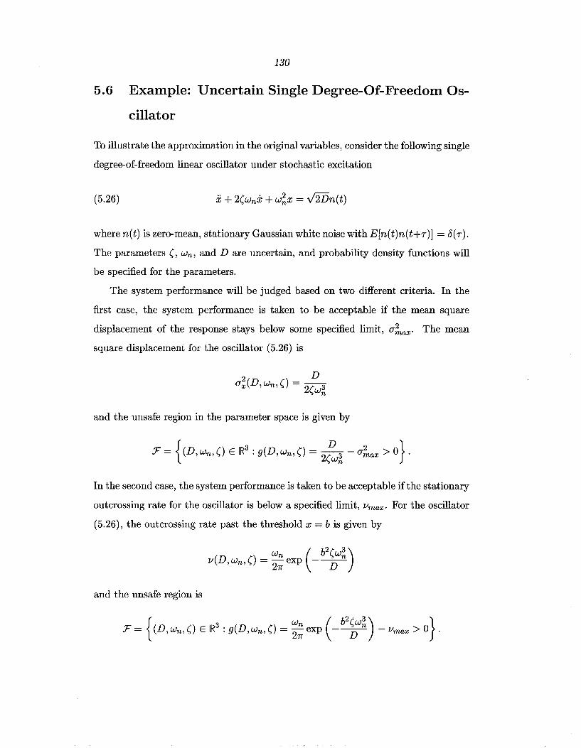
130

5.6 Example: Uncertain Single Degree-Of-Freedom Os­

cillator

To illustrate the approximation in the original variables, consider the following single

degree-of-freedom linear oscillator under stochastic excitation

(5.26)

where n(t) is zero-mean, stationary Gaussian white noise with E[n(t)n(t+T)] = 8(T).

The parameters (, wn, and D are uncertain, and probability density functions will

be specified for the parameters.

The system performance will be judged based on two different criteria. In the

first case, the system performance is taken to be acceptable if the mean square

displacement of the response stays below some specified limit, a~ax· The mean

square displacement for the oscillator (5.26) is

and the unsafe region in the parameter space is given by

{ a D 2 } F = (D, Wn, () E IR : g(D, Wn, () = 2(w~ - O"max > 0 ·

In the second case, the system performance is taken to be acceptable if the stationary

outcrossing rate for the oscillator is below a specified limit, Vmax. For the oscillator

(5.26), the outcrossing rate past the threshold x = b is given by

and the unsafe region is

131

5.6.1 Probability of exceeding mean square limit

First, consider the case where there only two uncertain parameters, Wn and (, so

that the methods can be easily visualized. These parameters are assumed to be

independently distributed and the probability density functions are chosen to be

lognormal distributions. The mean and variance parameters for the probability

density functions are chosen to be ffi( = ln0.05, mwn = ln27r, 0'( = 0.15, and O'wn =

0.05. The probability density functions are shown in Figure 5.5. The parameter D

is assumed to be known, with D = 2.

50 (\ 1.2

45

40

35 0.8

30 G ]: 0:25 0.0.6

20

0.4 15

10 \ 0.2

0 )

0 0 0.02 0.04 0.06 0.08 0.1 5

~ ro

Figure 5.5 Lognormal probability density functions for (and Wn·

For computing the probability that the mean square displacement is below a

specified limit, a~ax' the unsafe region is

{ 2 D 3 } :F = (wn,() E IR : g(wn,() = -

2 2 - (wn > 0 O'max

which is shown in Figure 5.6 for the case of a~ax = 0.15. The probability of fail­

ure is given by (5.20) with () = ((, wn) and p(O) = Pd()Pwn (wn)· Letting a = (,

'ljJ = Wn and h ( 'ljJ) = D / ( 2a'?nax 'ljJ3 ), the unsafe region is given by a < h ( 'ljJ) and

132

0.11 ,----,----,----,------.------;--,..---,-----,

0.08

0.07 s 0'0.06

0.05

0.04

F 0.03

0.02

0.01 4 4.5 5.5

Figure 5.6 Safe and unsafe regions for a; < 0.15

the failure probability can be obtained from (5.25), where Pa(-) is the cumulative

distribution function for (. The approximation can be easily obtained by solving a

one-dimensional unconstrained minimization problem to find the value of Wn maxi­

mizing the integrand.

Note that a different approximation can be obtained by applying (5.25) with

a= Wn, '1/J = (and h('lj.;) = (D/(2'1j.;O"~ax)) 113 • In the examples considered, it was

found that similar results were obtained by using either a = ( or a = Wn and results

are presented only for the asymptotic expansion applied to the integral when a = (.

Results are compared with those obtained by Breitung's method and the exact

values in Table 5.12 for various values of O"~ax· Breitung's method requires solving a

two-dimensional constrained minimization problem and then performing a number

of algebraic computations. Since the variables (wn, () are independently, lognormally

distributed, the transformation of variables to independent normal variables ( x1, x2)

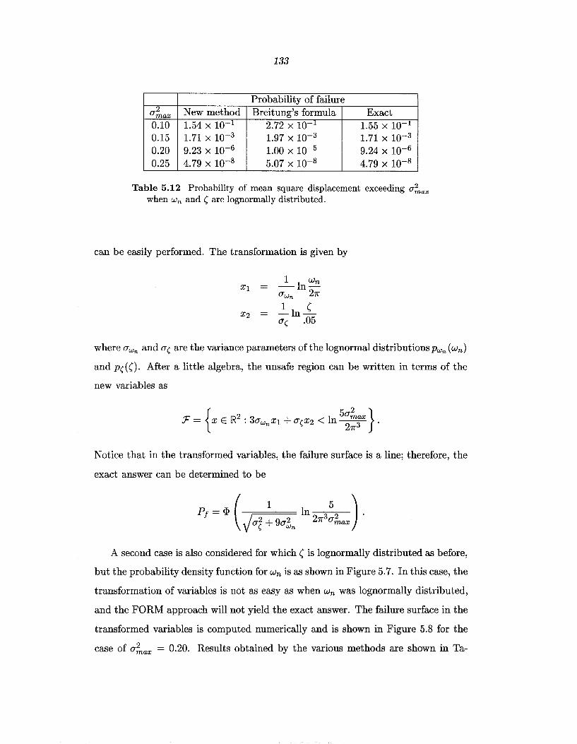
133

Probability of failure ,2

C!max New method Breitung's formula Exact 0.10 1.54 X 10 -l 2.72 X 10 ·l 1.55 X 10 -l

0.15 1.11 x 10-3 1.97 x 10-3 1.11 x 10-3

0.20 9.23 x 10-6 1.00 x w-5 9.24 x w-6

0.25 4.79 X 10-S 5.07 X 10-S 4.79 X 10-S

Table 5.12 Probability of mean square displacement exceeding cr~ax when Wn and ( are lognormally distributed.

can be easily performed. The transformation is given by

XI = _1_ln Wn C!wn 27r 1 (

x2 -ln-CF( .05

where cr wn and cr ( are the variance parameters of the lognormal distributions Pwn ( Wn)

and P(((). After a little algebra, the unsafe region can be written in terms of the

new variables as

Notice that in the transformed variables, the failure surface is a line; therefore, the

exact answer can be determined to be

A second case is also considered for which ( is lognormally distributed as before,

but the probability density function for Wn is as shown in Figure 5. 7. In this case, the

transformation of variables is not as easy as when Wn was lognormally distributed,

and the FORM approach will not yield the exact answer. The failure surface in the

transformed variables is computed numerically and is shown in Figure 5.8 for the

case of cr~ax = 0.20. Results obtained by the various methods are shown in Ta-

1.5

~ c:

8 a:

0.5

134

5.4 5.6 5.8 6.2 6.4 6.6 6.8

ron

Figure 5. 7 Probability density function Pwn (wn)

7.2

ble 5.13, along with the exact answers obtained by numerical integration. For both

of the probability density functions investigated, it is seen that the new approxima­

tion gives more accurate results than those obtained by Breitung's approximation,

especially for relatively large failure probabilities. The FORM approach gives the

exact result when Wn is lognormally distributed, but less accurate results than the

proposed approximation when Wn is distributed as in Figure 5.7.

Next, uncertainty in the excitation amplitude, D, is also considered. The param­

eter Dis taken to be lognormally distributed, with mv = ln2 and av = 0.1 and the

probability density function is illustrated in Figure 5.9. Results will be presented

only for the case when Wn and ( are lognormally distributed, as in Figure 5.5. The

resulting estimates for the probability of exceeding various bounds on the mean

square amplitude are shown in Table 5.14. As in the case when only Wn and (

were uncertain, the failure surface in the transformed variables is a plane, and the

exact answer can be obtained. The new approximation again gives more accurate

results than those obtained by Breitung's approximation, especially for relatively

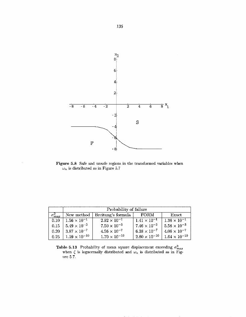
135

~ 8

6

4

2

-8 -6 -4 -2 2 4 6 8 xl

-2

s

F

Figure 5.8 Safe and unsafe regions in the transformed variables when Wn is distributed as in Figure 5. 7

Probability of failure

O"~ax New method Breitung's formula FORM Exact 0.10 1.56 X 10 1 2.92 X 10 -1 1.41 X 10 -1 1.38 X 10 -1

0.15 5.49 X 10-3 7.50 X 10-3 7.46 X 10-3 5.58 X 10-3

0.20 3.87 X 10-7 4.56 X 10-7 6.38 X 10-7 4.08 X 10-7

0.25 1.59 X 10-10 1.70 X 10-10 2.80 X 10-10 1.64 X 10-10

Table 5.13 Probability of mean square displacement exceeding a;;.,ax when ( is lognormally distributed and Wn is distributed as in Fig­ure 5.7.

1.8

1.6

1.4

1.2

e.1 c.

0.8

0.6

0.4

0.2

136

OL-~~~~~---L---L--~--~--~~~~

1 1.2 1.4 1.6 1.8 2 2.2 2.4 2.6 2.8

D

Figure 5.9 Probability density function for D.

large failure probabilities.

5.6.2 Probability of exceeding outcrossing rate limits

The first case considered is when only Wn and ( are uncertain and lognormally dis­

tributed, as shown in Figure 5.5. For computing the probability that the outcrossing

Probability of failure

O"~ax New method Breitung's formula Exact 0.10 1.76 x w-1 3.10 x w-1 1.so x w- 1

0.15 4.02 x w-3 4.62 x w-3 4.06 x w-3

0.20 5.32 X 10-5 5.73 X 10-5 5.36 X 10-5

0.25 6.94 X 10-7 7.31 X 10-7 6.99 X 10-7

Table 5.14 Probability of mean square displacement exceeding a~ax when D, Wn, and (are lognormally distributed.

137

rate exceeds a specified limit, Vmax, the unsafe region is

which is illustrated in Figure 5.10 for the case when the threshold b = 2 and Vmax = w-5.

0.09

0.08

0.07

0.06

'-1'0.05 s

0.04

0.03

F 0.02

0.01 4 4.5 5.5

Figure 5.10 Safe and unsafe regions for Vmax = w-5 .

The probability of failure can again be approximated by (5.25) with a = (, 'ljJ =

Wn, and h('lj;) = D/(b2'lj;3 ) ln(wn/(27rVmax)). Results are compared with Breitung's

formula and the FORM approach in Tables 5.15 and 5.16. It is again seen that

the new approximation gives more accurate results than Breitung's approximation.

In applying the FORM approach for this example with both variables lognormally

distributed, the failure surface is not a line, but can be very well approximated by a

line in the vicinity of the design point, as illustrated in Figure 5.11. For this reason,

the FORM approach gives very accurate estimates, as seen in Table 5.15. However,

the FORM results are not as accurate when Wn is distributed as in Figure 5.7, as

illustrated by the results in Table 5.16.

138

~ 8

6

4

2

-8 2 4 6 8 xl

-2

s

F

-8

Figure 5.11 Safe and unsafe regions in the transformed variables for Vmax = 10-5

Probability of failure Vmax New method Breitung's formula FORM Exact 10 -S 7.81 X 10 -2 1.15 X 10 -l 7.85 X 10 -2 7.85 X 10 -:.: w-7 2.oo x w-2 2.53 x w-2 2.oo x w-2 2.oo x w-2 w-6 2.61 x w-3 3.04 x w-3 2.62 x w-3 2.61 x w-3 w-s 1.20 x w-4 1.33 x w-4 1.21 x w-4 1.20 x w-4 w-4 9.85 x w-7 1.06 x w-6 9.86 x w-7 9.86 x w-7

Table 5.15 Probability of outcrossing rate exceeding specified limit Vmax

when ( and Wn are lognormally distributed.

139

Probability of failure

I/ max New method Breitung's formula FORM Exact 10-~ 6.90 X 10 -~ 1.25 X 10 -1 7.37 x 10-~ 6.37 x 10-~ 10-7 1.31 x 10-2 2.11 x 10-2 1.45 x 10-2 1.21 x 10-2

10-6 1.00 x 10-3 1.39 x 10-3 1.21 x 10-3 1.01 x 10-3

10-5 1.66 x 10-5 2.01 x 10-4 2.30 x 10-5 1.73 x 10-5 10-4 1.99 x 10-8 2.28 x 10-8 3.39 x 10-8 2.10 x 10-8

Table 5.16 Probability of outcrossing rate exceeding specified limit Vmax

when ( is lognormally distributed and Wn is distributed as in Fig­ure 5.7.

Probability of failure

I/ max New method Breitung's formula FORM Exact 10 -~ 9.90 X 10 -~ 1.46 X 10 -1 1.01 X 10 -1 1.01 X 10 .1

10-7 3.14 x 10-2 3.99 x 10-2 3.19 x 10-2 3.19 x 10-2

10-6 5.80 x 10-3 6.75 x 10-3 5.86 x 10_3 5.86 x 10-3

10-5 4.59 x 10-4 5.06 x 10-4 4.63 x 10-4 4.63 x 10-4 10-4 8.96 x 10-6 9.53 x 10-6 9.03 x 10-6 9.03 x 10-6

Table 5.17 Probability of outcrossing rate exceeding Vmax when D, Wn,

and ( are lognormally distributed.

Next, uncertainty in D is also considered and the probability function for D is

shown in Figure 5.9. Results obtained by the various methods are compared with

the exact answer obtained by numerical integration in Table 5.17. Again, the failure

surface in the transformed variables is very nearly a line, and the FORM approach

gives very accurate estimates. The new asymptotic approximation again gives very

good results, even for large failure probabilities.

140

Chapter 6

Conclusions

Several methods have been presented for analyzing uncertain dynamical systems.

Computationally efficient methods have been developed for analyzing nonlinear dy­

namical systems under stochastic excitation and for evaluating the multi-dimensional

integrals which arise when studying systems with modeling uncertainties. All of the

methods give approximate solutions and examples have been presented illustrating

the accuracy of the approximations.

In chapter 4, three new methods were developed for estimating the stationary

probability density function and statistical quantities of interest for the response

of nonlinear dynamical systems under uncertain excitation. The methods are all

based on obtaining approximate solutions to the Fokker-Planck equation for the

system and differ from traditional methods, which are based on finding approximate

solutions to the stochastic differential equations for the system.

In the first method presented, probabilistic linearization, the Gaussian probabil­

ity density function which best solves the Fokker-Planck equation for the nonlinear

system of interest is found and taken as an approximation for the probability density

function for the nonlinear system. For systems with polynomial-type nonlinearities,

the method can be very efficiently applied. Additionally, it was shown that by using

simple weighting functions, good approximations could be obtained for both the

moments and outcrossing rates of nonlinear systems.

The second method presented, probabilistic nonlinearization, finds a nonlinear

141

system having a known solution to its Fokker-Planck equation whose probability

density function provides the best fit to the Fokker-Planck equation for the nonlin­

ear system of interest. The probability density function for the approximate non­

linear system is non-Gaussian. Since the probability density function for nonlinear

systems is known to be non-Gaussian, the hope is that the non-Gaussian approxi­

mation will provide a better fit to the tails of the distribution than that obtained

by Gaussian approximations. For the example considered, the probabilistic nonlin­

earization method was able to provide good approximations to mean square values

for the response as well as obtaining a better fit to the Fokker-Planck equation than

what could be obtained by Gaussian probability density functions. However, the

approximation did not do a good job in approximating the tails of the probability

density function or the stationary outcrossing rate, as illustrated in Figures 4.31

and 4.33.

In order to improve the estimates of the tails of the probability density function

and the outcrossing rates, a third approximation method was developed. In this

method, the probability density function was directly approximated, without trying

to find an "equivalent system." The approximate probability density functions are

non-Gaussian, can be easily and efficiently determined, and yield the exact answer

for nonlinear systems that have known solutions to the Fokker-Planck equation.

For the examples considered, this method gave accurate results for mean square

values and outcrossing rates, as well as providing the best fit to the Fokker-Planck

equation.

In chapter 5, approximate methods were developed for analyzing systems with

modeling uncertainty. The uncertainty is modeled probabilistically and a simple

asymptotic approximation is used to approximate the multi-dimensional integrals

which arise. The accuracy of the asymptotic expansion was illustrated with several

examples.

In section 5.2, the asymptotic method is applied to determine the second mo­

ments and outcrossing rates of uncertain nonlinear systems under uncertain ex­

citation. Two examples are given which illustrate the accuracy of the proposed

142

approximation. It is also observed that the modeling uncertainties have little effect

on the mean square values, but a very significant effect on the outcrossing rates,

and hence the probability of failure.

The asymptotic approximation is applied to classical reliability integrals in sec­

tions 5.4.3 and 5.5. One approach to approximating classical reliability integrals,

the SORM approach, is to first transform the variables to independent standard

normal variables, then approximate the failure surface in the transformed variables

by a paraboloid, and finally approximate the resulting integral in the transformed

variables. In section 5.4.3, the asymptotic approximation is shown to yield a simple

and accurate formula for approximating the integral in the transformed variables.

The main disadvantage with the SORM approach is that the variables need

to be transformed to standard normal variables. While this can always be done

in principle, in many cases the transformation can only be done numerically, in

which case a substantial computational effort may be required. Additionally, by

transforming the variables, the sensitivity of the results to the original variables is

not often clear. In order to avoid these difficulties, the asymptotic approximation

was applied in the original variables in section 5.5. The approximation developed is

considerably simpler than an existing approximation, and an example is presented

for which the accuracy of the new approximation compares favorably to that of the

existing approximation.

6.1 Future Work

Another area of future research is to try to develop efficient methods for approx­

imating the stationary probability density function for nonlinear multi-degree-of­

freedom systems under additive stochastic excitation. In order to do this, a method

for determining a good set of approximate probability density functions for multi­

degree-of-freedom systems needs to be developed. In addition, computing the norm

of the Fokker-Planck equation error can become computationally expensive for non­

linear multi-degree-of-freedom systems, making it difficult to determine the optimal

143

parameters for the approximate probability density functions. Since computing the

norm of the Fokker-Planck equation error requires evaluating a probability inte­

gral similar to those studied in chapter 5, the asymptotic approximations developed

could be used to efficiently evaluate the norm and thus enable the optimal param­

eters to be found. A further area of research is finding approximate probability

density functions for systems under parametric excitation.

Future work is also required to investigate the accuracy of the asymptotic ap­

proximations for integrals in many dimensions. The approximations showed good

accuracy for all of the examples studied in this work, but the largest problem con­

sidered involved only a five-dimensional integral. Further testing needs to be done

to examine how the accuracy of the approximations changes with the dimension of

the integral to be approximated.

144

Appendix A

Another Choice for the Function Q(x1)

This appendix contains an alternative choice for the function Q(xi) used in the

direct probability density function approximation method discussed in section 4.4.

The goal is to select Q(xi) so that the approximate method presented in section 4.4

is capable of producing the the exact answer for systems for which an exact answer

is known.

It was shown that choosing

gives the exact answer if the system is linearly damped. However, this approach

will not give the exact answer for other cases for which solutions are known. Here, a

different choice of Q(x1) is made which will give the exact solution to a more general

set of nonlinear systems with known solutions of the form

(A.l)

where

Note that (A.l) includes the linearly damped case by selecting j(H) = constant.

145

For the general second-order nonlinear oscillator of the form

(A.2)

the approximate probability density functions can be chosen as

where

(A.4)

(A.5)

The following lemma proves that if the approximate probability density functions

are chosen as above and the system is of the solvable type (A.l), then the method

will yield the exact solution for the stationary Fokker-Planck equation.

Lemma A.l If the nonlinear system (A.2} is of the form (A.l}, i.e.

then the probability density function given by (A.3), (A.4) and (A.5) gives the exact

solution to the stationary Fokker-Planck equation when () = 1.

Proof:

It will be shown that p(x1, x2 1()) satisfies the stationary Fokker-Planck equation

corresponding to the nonlinear system (A.l). First, recall from section 4.4 that

(A.6)

146

Evaluating the derivatives of p(x1, x2IO) gives

1 = =-Dj(x1, x2)p(x1, x2IO)

(A.7) - ](H(xl, x2)) x2 p(x1, x2IO)

and

and

so that

(A.8)

147

Combining (A.6), (A.7), and (A.8), and setting()= 1 gives

i.e., p(x1, x2IO = 1) satisfies the stationary Fokker-Planck equation. •

148

Appendix B

Some Technical Results

B.l Proof of Lemma 5.1

The integrand is given by

and a necessary condition for a maximum of h(y) is that

{B.l)

for all i = 1, ... , m. One solution is clearly y = 0. Assuming that ai -I aj for all

i -I j and noting that h(y) > 0 for ally E IRn, any other solution of {B.l) must be

of the form

f) = {0, ... , ±:iJr, ... , 0)

where Yr is such that

{B.2)

149

Note that this clearly requires ar < 0. In the statement of Lemma 5.1, it was given

that

(B.3) ¢( -{3)

ar<P(-,8) >-1forallr=1, ... ,m

and for {3 ~ 0 it can be shown that V z > 0

¢( -{3 + z) ¢( -{3) <P( -,8 + z) < <P( -,8)"

Combining the above expression with (B.3) and setting z = -!ariJ; gives

for all Yr E IR. Therefore, there can be no solutions to (B.2), and the only stationary

point is y = 0. In the proof of Lemma 5.2, it is verified that y = 0 is actually a

maximum.

In the case where ai · = aj for some i -=f. j, additional solutions to (B.1) could

exist in the form

y= (0, ... ,O,yi,Yj,O, ... ,0)

where y[ + YJ = "(2 and

It was shown above that there can be no solutions to the above equation, since

ai :~ =~~ > -1, and hence y = 0 is the only stationary point in this case as well.

150

B.2 Proof of Lemma 5.2

The function £(y) is given by

l(y) In <1\ ( -/3- ~ ~ aw~) + ln¢(y)

( 1 ~ 2 ) 1 2 m lncl> -/3-2 L.-takYk - 2IIYII - 2ln27r.

k=l

Straightforward computations yield

which, when evaluated at y = 0, simplifies to

(B.4)

Thus, \7\7 £(y*) is a diagonal matrix and each of the diagonal elements is negative,

i.e., V'V'£(y*) is negative definite. Therefore, y* = 0 is a maximum of the integrand,

and the determinant of L(y*) = - \7\7£(y*) can be determined by inspection of (B.4)

to be

* rrm ( ¢(-/3)) det L(y ) = i=l 1 + ai cl>( -{3) ·

B.3 Proof of Case 2 of Theorem 5.1

In this case, y = 0 is still a stationary point of the integrand, and there are additional

stationary points at y = (0, 0, ±/k, 0, ... , 0) for all k such that ak :t ::::~~ < -1, where

/k is the unique positive solution of

(B.5) ak ¢( -{3- ak!V2) = -cl>( -{3- ak!V2).

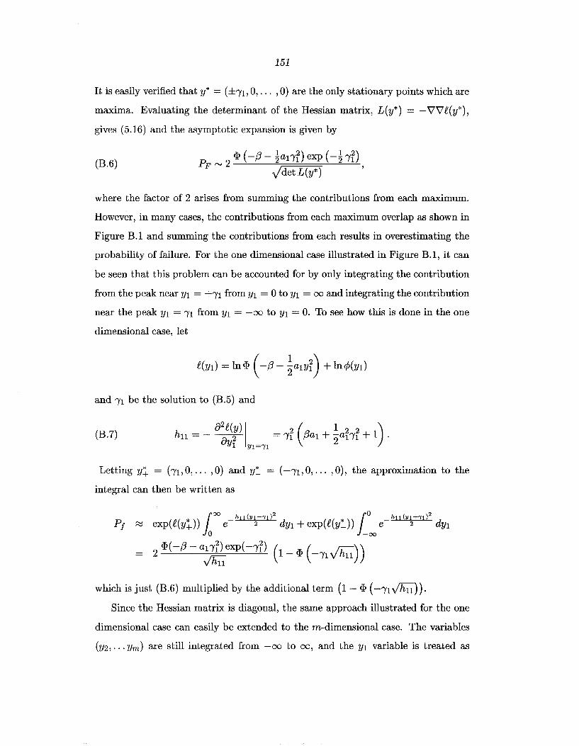
151

It is easily verified that y* = (±'n, 0, ... , 0) are the only stationary points which are

maxima. Evaluating the determinant of the Hessian matrix, L(y*) = -\7\7f(y*),

gives (5.16) and the asymptotic expansion is given by

(B.6) <P ( -!3- ~ant) exp ( -~ l't)

Pp rv 2 , Jdet L(y*)

where the factor of 2 arises from summing the contributions from each maximum.

However, in many cases, the contributions from each maximum overlap as shown in

Figure B.1 and summing the contributions from each results in overestimating the

probability of failure. For the one dimensional case illustrated in Figure B.l, it can

be seen that this problem can be accounted for by only integrating the contribution

from the peak near Y1 = +1'1 from Y1 = 0 to Y1 = oo and integrating the contribution

near the peak Y1 = /'1 from Y1 = -oo to Yl = 0. To see how this is done in the one

dimensional case, let

and /'1 be the solution to (B.5) and

(B.7)

Letting Y.+ = (1'1, 0, ... , 0) and y~

integral can then be written as

( -/'1, 0, ... , 0), the approximation to the

(£( *))100 _hJJ(YJ-'YJ)2 d (0( *))/_0 _hJJ(YJ+'YJ)2 d Pt ~ exp Y+ e 2 Y1 + exp {_ y_ e 2 Y1 0 -()()

2 <P( -!3- a1,;exp( -l'i) ( 1- <P ( -1'1 ~))

which is just (B.6) multiplied by the additional term (1- <P ( -1'1 Jhil)).

Since the Hessian matrix is diagonal, the same approach illustrated for the one

dimensional case can easily be extended to the m-dimensional case. The variables

(y2, ... Ym) are still integrated from -oo to oo, and the Y1 variable is treated as

oT I

co. I

:e

152

2~--~----~----~----~----~----~ -3 -2 -1 0

y1

Figure B. I Integrand for the probability of failure integral when (3 = 2 and a1 = -0.48.

above. Evaluating the integral gives

Pp "" 2 ci> ( -{3- ~anf) exp ( -~ 1D ( ( ~)) (B.8) Jdet L(y*) 1- ci> -')'1 Y hu

where det L(y*) is given by (5.16) and hu by (B.7).

B.4 Proof of Case 3 of Theorem 5.1

In this case, there is a surface of maxima of the integrand given by

where 'Y is such that

153

Since the Hessian matrix is singular at all of these points, the previous approach

will fail. However, a change of coordinates can be made to avoid this difficulty. Let

r 2 = y{ + ... y~ and notice that the terms in the integrand become

F(r, y)

J>(r,y)

The failure integral becomes

(B.9) 1 100 - - k 1 Pf = Ak-1 F(r, y)<!J(r, y) r - dr dyk+l · · · dyn

[Rn-k 0

where Ak is the surface area of the unit sphere ink-dimensions, given by (Flanders

1963)

21rk/2

Ak-1 = r(k/2).

The integrand in (B.9) has a unique maximum at (r*,y*) = (1,0), where 'Y is the

unique positive solution of

and the asymptotic method can be applied as before. The Hessian matrix is evalu­

ated to give

detL(y*) = ~ (2(k -1) + (k -1-"(2)(k -1-"(2h)) IT (1- ai). 'Y i=k+1 a1

Combining the results gives

(B.10) P 2(3-k)/2'Yk-1V'ff ip( -/3 _ ~an2) exp ( -~"!2)

F f'J r(k/2) y'det L(y*) ·

BIBLIOGRAPHY 154

Bibliography

Abramowitz, M. and I. A. Stegun (Eds.) (1964). Handbook of Mathematical Func­

tions with Formulas, Graphs, and Mathematical Tables, Volume 55 of Applied

Mathematics Series. National Bureau of Standards.

Andronov, A., L. Pontryagin, and A. Witt (1933). On the statistical investigation

of dynamical systems. Zh. Eksp. Tear. Fiz. 3, 165-180. (in Russian).

Arnold, L. (1974). Stochastic Differential Equations. Wiley - Interscience, New

York.

Atalik, T. S. and S. Utku (1976). Stochastic linearization of multi-degree-of­

freedom nonlinear systems. Earthquake Engineering and Structural Dynam­

ics 4, 411-420.

Atkinson, J.D. (1973). Eigenfunction expansions for randomly excited non-linear

systems. Journal of Sound and Vibration 30(2), 153-172.

Beck, J. L. (1989). Statistical system identification of structures. In Proceedings

5th International Conference on Structural Safety and Reliability, pp. 1395-

1402. ASCE.

Beck, J. L. (1996). System identification methods applied to measured seismic

response. In Proceedings of the 11th World Conference on Earthquake Engi­

neering, Acapulco.

Bendat, J. S., L. D. Enochson, G. H. Klein, and A. G. Piersol (1962). Advanced

concepts of stochastic processes and statistics for flight vehicle vibration es­

timation and measurement. Technical Report ASD-TR-62-1973, Flight Dyn.

Lab., Aero. Syst. Dir. Air Force System Command, Wright-Patterson Air

BIBLIOGRAPHY 155

Force Base, Ohio.

Bergman, L. A. and B. F. Spencer, Jr. (1992). Robust numerical solution of

the transient Fokker-Planck equation for nonlinear dynamical systems. In

N. Bellomo and F. Casciatti (Eds.), Nonlinear Stochastic Mechanics, pp. 49-

60. Berlin: Springer-Verlag.

Bergman, L.A., B. F. Spencer, Jr., S. F. Wojtkiewicz, and E. A. Johnson (1996).

Robust numerical solutions of the Fokker-Planck equation for second order

dynamical systems under parametric and external white noise excitations. In

W. Langford and W. K. and (Eds.), Nonlinear Dynamics and Stochastic Me­

chanics, Volume 9 of American Mathematical Society, pp. 23-37. Providence:

Fields Institute Communications.

Bleistein, N. and R. Handelsman (1986). Aymptotic Expansions for Integrals. New

York: Dover.

Bogdanoff, J. L. and F. Kozin ( 1961). Comment on reliability of aircraft structures

in resisting chance failure. Operations Research 9(1), 123-126.

Booton, R. C. (1954). Nonlinear control systems with random inputs. IRE Trans­

actions on Circuit Theory 1, 9-19.

Bouc, R. (1967). Forced vibration of mechancial systems with hysteresis. In Pro­

ceedings of the Fourth International Conference on Nonlinear Oscillations,

Prague, Czechoslovakia. (abstract).

Box, G. E. P. and G. C. Tiao (1973). Bayesian Inference in Statistical Analysis.

John Wiley and Sons, Inc.

Breitung, K. (1984). Asymptotic approximations for multinormal integrals. Jour­

nal of Engineering Mechanics, ASCE 110(3), 357-366.

Breitung, K. (1989). Asymptotic approximations for probability integrals. Prob­

abilistic Engineering Mechanics 4 (4), 187-190.

Bucher, C. G. (1988). Adaptive sampling- an iterative fast Monte Carlo proce­

dure. Structural Safety 5, 119-126.

BIBLIOGRAPHY 156

Caughey, T. K. (1959a). Response of a nonlinear string to random loading. ASME

Journal of Applied Mechanics 26(3), 341-344.

Caughey, T. K. (1959b). Response of a van der Pol oscillator to random excitation.

ASME Journal of Applied Mechanics 26(3), 345-348.

Caughey, T. K. (1963). Equivalent linearization techniques. Journal of the Acous­

tical Society of America 35, 1706-1701.

Caughey, T. K. (1971). Nonlinear theory of random vibrations. In C. S. Yih (Ed.),

Advances in Applied Mechanics, Volume 11, pp. 209-253. New York: Acaemic

Press.

Caughey, T. K. (1986). On the response of non-linear oscillators to stochastic

excitation. Probabilistic Engineering Mechanics 1 (1), 2-4.

Caughey, T. K. and F. Ma (1982). The exact steady-state response of a class of

nonlinear stochastic systems. International Journal of Non-Linear Mechan­

ics 49(3), 137-142.

Chandiramani, K. L. (1964). First-Passage Probabilities of a Linear Oscillator.

Ph. D. thesis, Department of Mechanical Engineering, Massachusetts Institute

of Technology, Cambridge, Massachusetts.

Chen, J. J. (1994). Analysis of engineering structures response to random wind

excitation. Computers f3 Structures 51 (6), 687-693.

Clarkson, B. L. and D. J. Mead (1972). High frequency vibration of aircraft

structures. Journal of Sound and Vibration 28, 487-504.

Coleman, J. J. (1959). Reliability of aircraft structures in resisting chance failure.

Operations Research 7(5), 639-645.

Cramer, H. (1966). On the intersections between the trajectories of a normal

stationary stochastic process and a high level. Arkiv fOr Matematik 6, 337-

349.

Crandall, S. H. (1963). Perturbation techniques for random vibration of nonlinear

systems. Journal of the Acoustical Society of America 35, 1700-1705.

BIBLIOGRAPHY 157

Crandall, S. H. (1970). First crossing probabilities of the linear oscillator. Journal

of Sound and Vibration 12(3), 285-299.

Crandall, S. H. (1980). Non-Gaussian closure for random vibration excitation.

International Journal of Non-Linear Mechanics 15(4/5), 303-313.

Crandall, S. H., K. L. Chandiramani, and R. G. Cook (1966). Some first-passage

problems in random vibration. ASME Journal of Applied Mechanics 33, 532-

538.

Crandall, S. H. and W. D. Mark (1963). Random Vibrations in Mechanical Sys­

tems. Academic Press.

Darling, D. A. and A. J. F. Siegert (1953). The first passage problem for a con­

tinuous Markov process. Annals of Mathematical Statistics 24, 624-639.

Davenport, A. G. and M. Novak (1976). Vibration of structures induced by wind.

In C. M. Harris and C. E. Crede (Eds.), Shock and Vibration Handbook, Chap­

ter 29. McGraw-Hill.

Der Kiureghian, A., H. Z. Lin, and S. J. Hwang (1987). Second-order reliability ap­

proximations. Journal of Engineering Mechanics, ASCE 113(8), 1208-1225.

DiPaola, M. and G. Falsone (1997). Higher order statistics of the response of

mdof linear systems excited by linear parametric white noises and external

excitations. Probabilistic Engineering Mechanics 12(3), 179-188.

Dunne, I. F. and J. H. Wright (1985). Predicting the frequency of occurrence of

large roll angles in irregular seas. Proceedings of the Royal Institution of Naval

Architects 127, 233-245.

Dunne, J. F. (1996). An optimal-control approach to extreme local maxima for

stochastic Duffing-type oscillators. Journal of Sound and Vibration 193(3),

597-629.

Elishakoff, I. and G. Q. Cai (1993). Approximate solution for nonlinear random

vibration problems by partial stochastic linearization. Probabilistic Engineer­

ing Mechanics 8, 233-237.

BIBLIOGRAPHY 158

Falsone, G. (1992). Stochastic linearization of mdof systems under parametric

excitation. International Journal of Non-Linear Mechanics 27(6), 1025-1037.

Feller, W. (1968). An Introduction to Probability Theory and Its Applications,

Volume 1. John Wiley & Sons.

Feng, M. Q. and R. C. Zhang (1997). Wind-induced vibration characteristics of

Nanjing TV tower. International Journal of Non-Linear Mechanics 32(4),

693-706.

Fischera, G. (1960). On a unified theory of boundary value problems for elliptic­

parabolic equations of a second order. In R. E. Langer (Ed.), Boundary Prob­

lems in Differential Equations, pp. 97-102. University of Wisconsin Press.

Flanders, H. (1963). Differential Forms with Applications to the Physical Sciences.

Dover.

Fokker, A. (1915). Ann. Phys. (Leipzig) 43, 310.

Foster, E. T. (1968). Semi-linear random vibrations in discrete systems. ASME

Journal of Applied Mechanics 35, 560-564.

Gardiner, C. W. (1994). Handbook of Stochastic Methods for Physics, Chemistry

and the Natural Sciences. Springer-Verlag.

Gawthrop, P. J., A. Kountzeris, and J. B. Roberts (1988). Parametric identifi­

cation of nonlinear ship motion from forced roll data. Journal of Ship Re­

search 32, 101-111.

Gihman, I. I. and A. V. Skorohod (1975). The Theory of Stochastic Processes,

Volume I,II,III. Springer, New York.

Grigoriu, M. and B. Allbe (1986). Response of offshore structures to waves. Jour­

nal of Engineering Mechanics, ASCE 112, 729-744.

Hamamoto, T. (1995). Stochastic fluid-structure interaction of large circular float­

ing islands during wind-waves and seaquakes. Probabilistic Engineering Me­

chanics 10(4), 209-224.

BIBLIOGRAPHY 159

Hijawi, M., R. A. Ibrahim, and N. Moshchuk (1997). Nonlinear random response

of ocean structures using first-order and 2nd-order stochastic averaging. Non­

linear Dynamics 12(2), 155-197.

Hohenbichler, M. and R. Rackwitz (1988). Improvement of second-order relia­

bility estimates by importance sampling. Journal of Engineering Mechanics,

ASCE 114 (12), 2195-2198.

Hu, S. L. J. and D. S. Zhao {1993). Non-Gaussian properties of 2nd-order random

waves. Journal of Engineering Mechanics, ASCE 119(2), 344-364.

Hunt, H. E. M. (1996). Modelling of rail vehicles and track for calculation of

ground-vibration transmission into buildings. Journal of Sound and Vibra­

tion 193(1), 185-194.

Ibrahim, R. A. (1985). Parametric Random Vibration. Taunton, UK: Research

Studies Press.

Islam, M.S., B. Ellingwood, and R. B. Corotis (1992). Wind-induced response of

structurally asymmetric high-rise buildings. Journal of Structural Engineer­

ing 118(1), 207-222.

Ito, K. {1951). On stochastic differential equations. Memoirs of the American

Mathematical Society 4, 289-232.

Iwan, W. D. (1973). A generalization of the concept of equivalent linearization.

International Journal of Nonlinear Mechanics 8, 279-287.

I wan, W. D. {1974). Application of nonlinear analysis techniques. In W. D. Iwan

{Ed.), Applied Mechanics in Earthquake Engineering, Volume 8 of AMD.

American Society of Mechanical Engineers.

Iwan, W. D. and I. M. Yang (1972). Application of statistical linearization tech­

niques to nonlinear multi-degree-of-freedom systems. Journal of Applied Me­

chanics 39, 545-550.

Jahedi, A. and G. Ahmadi {1983). Application of Wiener-Hermite expansion

to nonstationary random vibration of a du:ffing oscillator. ASME Journal of

BIBLIOGRAPHY 160

Applied Mechanics 50(2), 436-442.

Jeffreys, H. (1961). Theory of Probability. Oxford Clarendon Press.

Kanai, K. (1957). Semi-empirical formula for the seismic characteristics of the

ground. Bulletin of the Earthquake Research Institute (Tokyo University) 35,

309-325.

Kareem, A. (1992). Dynamic-response of high-rise buildings to stochastic wind

loads. Journal of Wind Engineering 42, 1101-1112.

Katafygiotis, L. S., C. Papadimitriou, andY. Tsarkov (1997). Mean-square sta­

bility of linear stochastic dynamical systems under parametric wide-band ex­

citations. Probabilistic Engineering Mechanics 12(3), 137-147.

Kirk, C. L. (1974). Application of the Fokker-Planck equation to random vi­

bration of non-linear systems. Technical Report 20, Cranfield Institute of

Technology, U. K.

Kolmogorov, A. N. (1931). Math. Anal. 104, 415-418.

Koyliioglu, H. U. and S. R. K. Nielsen (1994). New approximations for SORM

integrals. Structural Safety 13, 235-246.

Kunert, A. (1991). Efficient numerical solution of multidimensional Fokker­

Planck equations with chaotic and nonlinear random vibration. In T. C.

Huang, C. S. Hsu, W. Q. Feng, S. C. Sinha, R. A. Ibrahim, and R. L. Engelstad

(Eds.), Vibrational Analysis -Analytical and Computational, Volume 37.

Langatangen, H. P. (1991). A general numerical solution method for Fokker­

Planck equations with applications to structural reliability. Probabilistic En­

gineering Mechanics 6(1), 33-48.

Langevin, P. (1908). Comptes. Rendues 146, 530.

Langley, R. S. (1985). A finite element method for the statistics of non-linear

random vibration. Journal of Sound and Vibration 101 (1), 41-54.

Leira, B. J. (1987). Multidimensional stochastic linearization of drag forces. Ap­

plied Ocean Research g, 150-162.

BIBLIOGRAPHY 161

Lin, Y. K. (1967). Probabilistic Theory of Structural Dynamics. McGraw Hill.

Lin, Y. K. and G. Q. Cai (1988). Exact stationary-response solution for second­

order nonlinear systems under parametric and external white-noise excita­

tions. Part II. ASME Journal of Applied Mechanics 55(3), 702-705.

Lin, Y. K. and G. Q. Cai (1995). Probabilistic Structural Dynamics: Advanced

Theory and Applications. McGraw-Hill, Inc.

Lutes, L. D. (1970). Approximate technique for treating random vibration of

hysteretic systems. Journal of the Acoustical Society of America 48(1), 299-

306.

Lutes, L. D. and S. Sarkani (1997). Stochastic Analysis of Structural and Mechan­

ical Vibrations. Prentice Hall.

Madsen, H. 0., S. Krenk, and N. C. Lind (1986). Methods of Structural Safety.

Prentice-Hall.

May, B. S. (1997). Probabilistic Robust Control: Theory and Applications. Ph. D.

thesis, California Institute of Technology.

Naess, A. and J. M. Johnsen (1991). Response statistics of nonlinear dynamic sys­

tems by path integration. In Proceedings of IUTAM Symposium on Nonlinear

Stochastic Mechanics, Torino, Italy.

Newland, D. E. (1986). General linear theory of vehicle response to random road

roughness. In I. Elishakoff and R. H. Lyon (Eds.), Random Vibration- Status

and Recent Developments, pp. 303-326. Elsevier.

Newland, D. E. (1993). An Introduction to Random Vibrations, Spectral €3

Wavelet Analysis. Longman Scientific & Technical.

Nigam, N.C. (1983). Introduction to Random Vibrations. Cambridge: MIT Press.

Papadimitriou, C. and J. L. Beck (1994). Approximate random vibration anal­

ysis of classically damped mdof systems. Journal of Engineering Mechanics,

ASCE 120(1), 75-96.

BIBLIOGRAPHY 162

Papadimitriou, C., J. L. Beck, and L. S. Katafygiotis (1995). Asymptotic expan­

sions for reliabilities and moments of uncertain dynamical systems. Technical

Report EERL95-05, Earthquake Engineering Research Laboratory,California

Institute of Technology, Pasadena, CA.

Papadimitriou, C., J. L. Beck, and L. S. Katafygiotis (1997). Asymptotic expan­

sions for reliabilities and moments of uncertain dynamic systems. Journal of

Engineering Mechanics, ASCE 123(12). To appear.

Papadimitriou, C. and L. D. Lutes {1996). Stochastic cumulant analysis of mdof

systems with polynomial type nonlinearities. Probabilistic Engineering Me­

chanics 11 (1), 1-13.

Park, Y. J. (1992). Equivalent linearization for seismic responses. 1. Formulation

and error. Journal of Engineering Mechanics, ASCE 118(11), 2207-2226.

Planck, M. (1917). Sitzungsber. Pruess. Akad. Wiss. Phys. Math. K1. 325.

Polidori, D. C. and J. L. Beck (1996). Approximate solutions for nonlinear random

vibration problems. Probabilistic Engineering Mechanics 11(2), 179-185.

Press, H. and J. C. Houboult (1955). Some applications of generalized harmonic

analysis to gust loads on airplanes. Journal of the Aero/Space Sciences 22,

17-26.

Redhorse, J. R. and P. D. Spanos (1992). A generalization to stochastic averaging

in random vibration. International Journal of Non-Linear Mechanics 27(1),

85-101.

Rice, S. 0. (1944). Mathematical analysis of random noise. Bell System Technical

Journal 23, 282-332. Reprinted in Selected Papers in Noise and Stochastic

Processes, ed. N. Wax, Dover, New York, 1954.

Risken, H. (1989). The Fokker-Planck Equation. Methods of Solution and Appli­

cations. Springer-Verlag.

Roberts, J. B. (1978a). First-passage time for oscillators with nonlinear damping.

ASME Journal of Applied Mechanics 45, 175-180.

BIBLIOGRAPHY 163

Roberts, J. B. (1978b). First-passage time for oscillators with nonlinear restoring

forces. Journal of Sound and Vibration 60, 177-185.

Roberts, J. B. (1982). A stochastic theory for non-linear ship rolling in irregular

seas. Journal of Ship Research 26, 229-245.

Roberts, J. B. and P. D. Spanos (1990). Random Vibration and Statistical Lin­

earization. Wiley, New York.

Rosenblatt, M. (1952). Remarks on a multivariate transformation. The Annals of

Mathematical Statistics 23, 470-472.

Rudin, W. (1987). Real and Complex Analysis. McGraw-Hill, Inc.

Schiehlen, W. 0. (1986). Random vehicle vibrations. In I. Elishakoff and R. H.

Lyon (Eds.), Random Vibration - Status and Recent Developments, pp. 379-

388. Elsevier.

Schueller, G. I., M. D. Pandey, and H. J. Pradlwarter (1994). Equivalent lin­

earization in engineering practice for aseismic design. Probabilistic Engineering

Mechanics 9, 95-102.

Schueller, G. I. and R. Stix (1987). A critical appraisal of methods to determine

failure probabilities. Structural Safety 4, 293-309.

Soize, C. (1994). The Fokker-Planck Equation for Stochastic Dynamical Systems

and its Explicit Steady State Solutions. World Scientific.

Soong, T. T. and M. Grigoriou (1993). Random Vibration of Mechanical and

Structural Systems. Prentice-Hall International.

Spencer, Jr., B. F. and L.A. Bergman (1991). Numerical solution of the Fokker­

planck equation for first passage probabilities. In P. D. Spanos and C. A. Breb­

bia (Eds.), Computational Stochastic Mechanics, pp. 359-370. Southamption:

Computational Stochastic Publications/ Elsevier.

Spencer, Jr., B. F. and L.A. Bergman (1993). Numerical solutions ofthe Fokker­

Planck equation for nonlinear stochastic systems. Nonlinear Dynamics 4, 357-

372.

BIBLIOGRAPHY 164

Stratonovich, R. L. (1963). Introduction to the Theory of Random Noise, Vol­

ume 1. Gordon and Breach.

Sun, J. Q. and C. S. Hsu (1988). First-passage time probability of non-linear

stochastic systems by generalized cell mapping method. Journal of Sound and

Vibration 124, 233-248.

Sun, J. Q. and C. S. Hsu (1990). The generalized cell mapping method in nonlinear

random vibrations. ASME Journal of Applied Mechanics 124, 233-248.

Tajimi, H. (1960). A statistical method of determining the maximum response of a

building structure during an earthquake. In Proceedings 2nd World Conference

on Earthquake Engineering, Volume II, Tokyo and Kyoto, Japan, pp. 781-798.

Thoft-Christensen, P. andY. Murotsu (1986). Application of Structural Systems

Reliability Theory. Springer-Verlag.

Trebicki, J. and K. Sobczyk (1996). Maximum-entropy principle and non­

stationary distributions of stochastic systems. Probabilistic Engineering Me­

chanics 11 (3), 169-178.

Tvedt, L. (1983). Two second-order approximations to the failure probability.

Technical Report RDIV /20-004-83, Det Norske Veritas, Oslo, Norway.

Ushkalov, V. F. (1986). Random vibrations of railway vehicles. In I. Elishakoff

and R. H. Lyon (Eds.), Random Vibration- Status and Recent Developments,

pp. 379-388. Elsevier.

Vanmarcke, E. H. (1976). Structural response to earthquake. In C. Lomnitz and

E. Rosenblueth (Eds.), Seismic Risk and Engineering Decisions, Chapter 8.

Elsevier.

Visintin, A. (1994). Differential Models of Hysteresis. Springer.

Wen, Y. K. (1975). Approximate method for nonlinear random vibration. Jmtrnal

of the Engineering Mechanics Division, ASCE 101 (EM4), 389-401.

Wen, Y. K. (1976). Method for random vibration of hysteretic systems. Journal

of the Engineering Mechanics Division, ASCE 102(EM2), 249-263.

BIBLIOGRAPHY 165

Wen, Y. K. (1980). Equivalent linearization for hysteretic systems under random

excitation. ASME Journal of Applied Mechanics 47(1), 150-154.

Wiener, N. (1923). Differential space. Journal of Math and Physics 2, 131-174.

Wojtkiewicz, S. F., L. A. Bergman, and B. F. Spencer, Jr. (1995). Numerical

solution of some three-state random vibration problems. In Proceedings of

the Fifteenth Biennial Conference on Mechanical Vibrations and Noise, pp.

939-947.

Wojtkiewicz, S. F., B. F. Spencer, and L.A. Bergman (1996). On the cumumlant­

neglect closure method in stochastic dynamics. International Journal of Non­

Linear Mechanics 31 (5), 657-684.

Wolfram, S. (1991). Mathematica, A System for Doing Mathematics by Computer.

Addison-Wesley.

Wong, E. and M. Zakai (1965). On the relation between ordinary and stochas­

tic differential equations. International Journal of Engineering Sciences 3(2),

213-229.

Yang, C.-M. and J. L. Beck (1998). Generalized trajectory methods for finding

multiple extrema and roots of functions. Journal of Optimization Theory and

Applications. To appear in April.

Yang, J.-N. and M. Shinozuka (1970). First passage time problem. The Acoustical

Society of America 47(2), 393-394.

Yong, Y. and Y. K. Lin (1987). Exact stationary-response solution for second­

order nonlinear systems under parametric and external white-noise excita­

tions. ASME Journal of Applied Mechanics 54 (2), 414-418.

Yoon, Y. J. and R. A. Ibrahim (1995). Parametric random-excitation of nonlinear

coupled oscillators. Nonlinear Dynamics 8(3), 385-413.