Embed Size (px)
Citation preview

Evolvable Hardware

2
EWH
• EHW: A bio-inspired technique for hardware design.
• Living beings: DNA constitute the encoding of every living being on
the Earth.− ACTG strings.
• Reconfigurable logic: Bitstream determines the logic.
− 01 strings.

3
Living Beings vs. Circuits
In DNA, the amount of guanine is equal to cytosine and the amount of adenine is equal to thymine. The A:T and C:G pairs are structurally similar.

4
POE Model
• The space of artificial bio-inspired systems can be partitioned along these three axes.
1. Phylogeny: Temporal evolution of a certain genetic material in
individuals and species.− Evolutionary algorithms (EA): simplified artificial counterpart
of phylogeny in nature.− Mutation, Crossover, ….
2. Epigenesis: Learning process during an individual’s lifetime.
− ANNs: the system’s synaptic weights change through interactions with the environment.
3. Ontogeny: Development of a single individual from its own genetic
material (without environmental interaction).− Self-replicating and self-repairing cellular automata.

5
Epigenesis
• Artificial neural network (ANN): Massively parallel distributed computing units made up
of very simple basic elements. Feature: Storing experiential knowledge making it
available for future use. Inspired from animals’ brains:
− Benefit from a massively parallel cellular architecture.− A learning process allows acquiring a certain knowledge.− This knowledge is stored in the form of synaptic weights
interconnecting neurons. Able to compute nonlinear input-output functions. Adaptable (adjustable synaptic weights and network
topology can adapt to its operating environment).
6
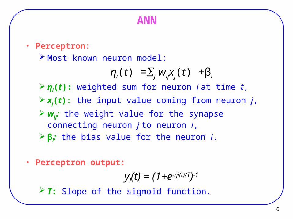
ANN
• Perceptron: Most known neuron model:
ηi(t) =j wijxj(t) +βi
ηi(t): weighted sum for neuron i at time t,
xj(t): the input value coming from neuron j,
wij: the weight value for the synapse connecting neuron j to neuron i,
βi: the bias value for the neuron i.
• Perceptron output:
yi(t) = (1+e-ηi(t)/T)-1
T: Slope of the sigmoid function.

7
ANN Supervised Learning
• Artificial neural network
Supervised learning

8
ANN Unsupervised Learning
• Unsupervised learning: There is no information about the task to be performed,
synaptic modifications depend on correlations among input data.
• Applications: Clustering, Pattern recognition, Reconstruction of corrupted data, ….

9
Genetic Algorithms
• GA: An iterative procedure applied to a constant-size
population of individuals. Each individual represents a possible solution.
− Eventually one is chosen. Each individual is coded by a finite string of symbols
known as the genome. Each genome gives rise to the individual’s phenotype,
which constitutes the actual solution (e.g. a circuit) to the problem at hand (e.g., a robot controller).
The individual receives a score (fitness) depending on the performance exhibited during its evaluation.
10
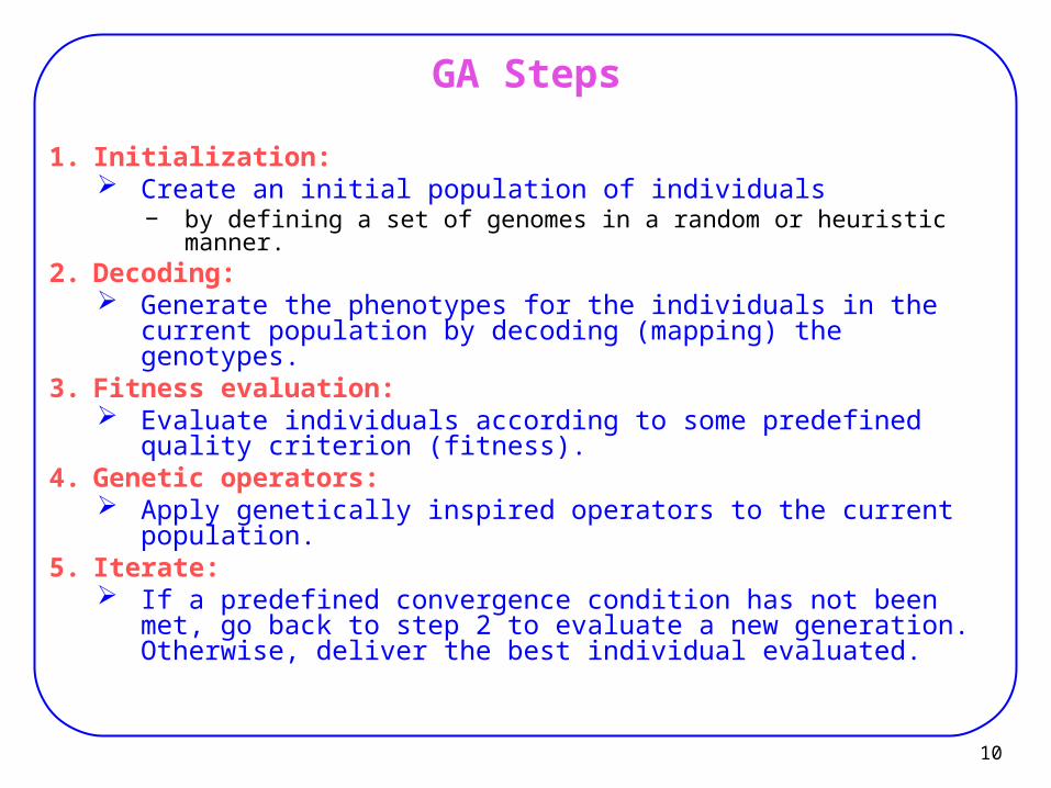
GA Steps
1. Initialization: Create an initial population of individuals
− by defining a set of genomes in a random or heuristic manner.2. Decoding:
Generate the phenotypes for the individuals in the current population by decoding (mapping) the genotypes.
3. Fitness evaluation: Evaluate individuals according to some predefined quality
criterion (fitness).4. Genetic operators:
Apply genetically inspired operators to the current population.5. Iterate:
If a predefined convergence condition has not been met, go back to step 2 to evaluate a new generation. Otherwise, deliver the best individual evaluated.

11
Genetic Operators
• Selection: Individuals are selected into a mating pool for
reproduction according to their fitness. − Stochastic or deterministic selection.
• Crossover: Two genomes are selected to be split and swapped at
a random position.
• Mutation: The genome is randomly changed.

12

13
Conventional Circuit Design
• Circuit design: A hard engineering task Vulnerable to human error, For large circuits the optimality of a solution cannot be
guaranteed. Design automation has become a challenge. Increasing complexity of circuits Higher abstraction levels
needed.
EWH: a solution

14
Evolutionary Circuit Design
• EHW:
From a given behavior specification of a circuit, an EA will search for a bitstream describing a circuit that satisfies it.
− Most works: application of EAs to synthesis.
− Evolutionary circuit design is more descriptive than EHW.

15
Evolutionary Circuit Design
• Major advantage: Designer’s job is reduced to constructing the
evolutionary setup: Specifying 1. Circuit requirements,
2. Basic elements,
3. A decoding mechanism,
4. Testing scheme used to assign fitness − often the most difficult.
Automatic generation of the circuit.

16
EWH
• Two critical questions when setting up a system:
1. How to map a phenotype from a genotype?
2. How to compute the fitness of a circuit?

18
Low-Level Languages
• Low-level languages− Directly incorporating the bit string representing the
configuration of a programmable circuit within the genome• Genome encoding steps:
A set of basic logic gates must be chosen (e.g., AND, OR, and NOT)
and codified along with the interconnections between gates• Problems:
Genome’s length: order of tens of thousands of bits,− Evolution practically impossible
Many circuits are invalid.• Solutions by XC6200:
MUX-based Direct correspondence between the bit string of a cell and the actual logic circuit.
Separate configuration of each cell Remarkedly faster
19
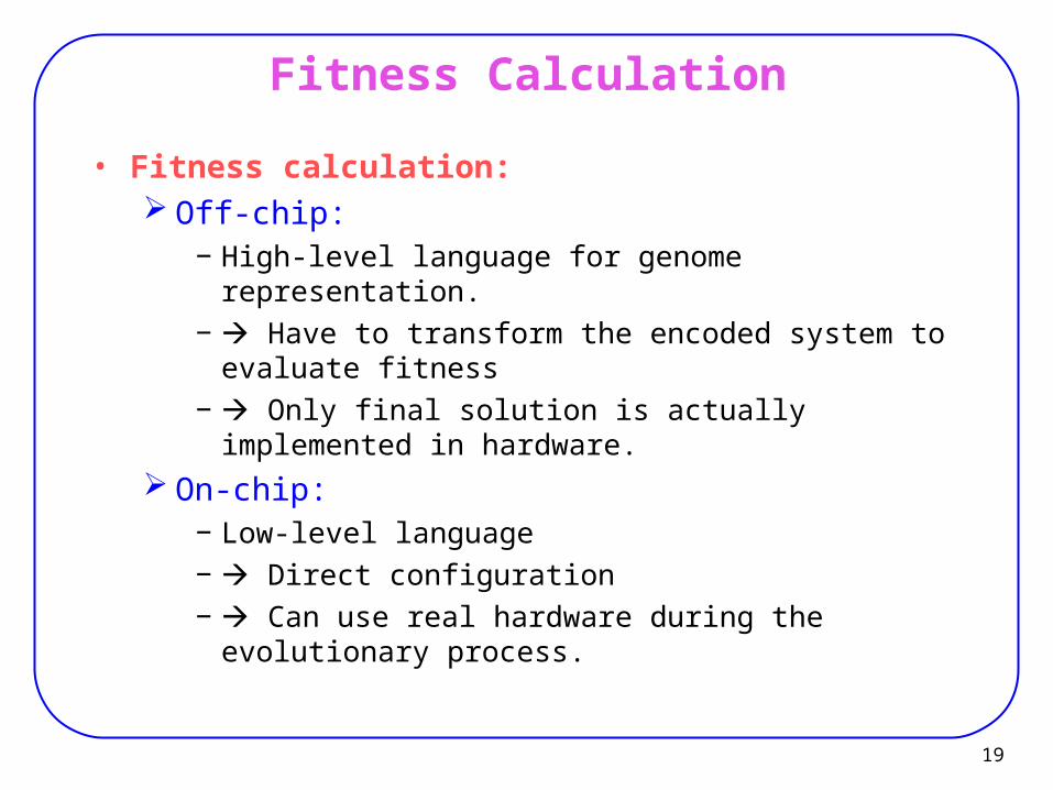
Fitness Calculation
• Fitness calculation: Off-chip:
− High-level language for genome representation.− Have to transform the encoded system to evaluate
fitness− Only final solution is actually implemented in
hardware. On-chip:
− Low-level language− Direct configuration− Can use real hardware during the evolutionary
process.

20
EHW Classification
• Classes acc. to the level of bio-inspiration:

21
Extrinsic Evolution
• Extrinsic evolution: All operations are carried out in software, Solution possibly loaded into a real circuit.
− Traditional evolutionary techniques for synthesis. At different abstraction levels
− Scheduling and allocation,− Logic synthesis,− Placement and routing.
Not suitable for evolving at bitstream level.

22
Intrinsic Evolution
• Intrinsic evolution: A real circuit is used during the evolutionary process
for output computation, Most operations are still carried out in software.

23
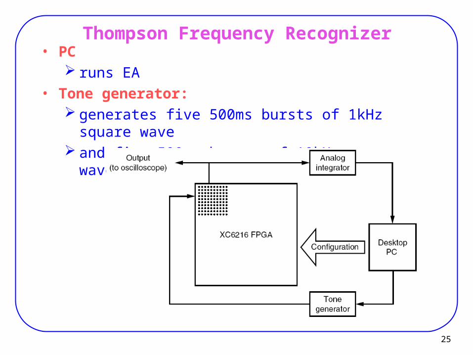
Thompson Frequency Recognizer
• FPGA:Xilinx XC6216
A 10x10 corner of 64x64 array was used.
No configuration can damage the device.
− EA can manipulate configuration without legality constraints or checking.
Configuration: 1800 bits.

24
Thompson Frequency Recognizer
• Circuit: Discriminate between 1kHz and 10kHz tones.
• Aim: Output goes to 5v when one tone appears at input. Output goes to 0v otherwise.
• GA: Population size: 50 Individuals: 1800-bit strings Initial population: random Next generation:
− Copy the fittest individual− Crossover rate: 70%− Number of mutations per genotype: 2.7
25
Thompson Frequency Recognizer• PC
runs EA
• Tone generator: generates five 500ms bursts of 1kHz square wave and five 500ms bursts of 10kHz square wave

26
Thompson Frequency Recognizer
• Inputs to circuit: 10 test tones shuffled randomly
500ms 500ms
11 12 110
• FPGA: takes test tones generate outputs

27
Thompson Frequency Recognizer
500ms 500ms
11 12 110
• Integrator: integrates FPGA outputs over 500ms generates it for test tone number t (t = 1,2, …, 10)
• Fitness:
• S1:
set of five 1kHz tones
• S10:
set of five 10kHz tones
k1=1/30730,
k2=1/30527

28
Thompson Frequency Recognizer
• Objective: Maximizing the difference:
− average output voltage when 1kHz input is present and− average output voltage when 1kHz input is present.

29
• Oscilloscope screen for best individual in
some generations
• Experiment time: 2-3 weeks no human time

30
Final Circuit

31
Final Circuit

33
Intrinsic Evolution
• Problem: Large genome size.
• Solutions: Variable-length chromosome GAs (VGA):
− Genome does not directly represent the configuration bit string but rather codifies the possible logical operations and interconnections.
Evolution at the function level:− Basic units are not elementary logic gates (e.g., AND,
OR, and NOT) but rather higher-level functions (e.g. sine-wave generator, multiplier).
− Problem: No such commercial FPGA− Solution: [Murakawa96] proposed F2PGA (Function-
based FPGA)

34
Complete Evolution• Complete evolution:
All operations (selection, crossover, mutation) and fitness evaluation, are carried out intrinsically, in hardware.− Different from biological evolution: not open ended:
− There is a predefined goal.
• Two types:
1. Centralized
2. Population-oriented

35
Complete Evolution
• Centralized evolution: There is a single evolvable
circuit and a single evolvable algorithm computation:
− EA is executed in an on-chip processor.
Popular− because it greatly enhances
the autonomy of the circuit− EHW can adapt to a changing
environment during its lifetime.

36
Complete Evolution
• Centralized evolution: Implementations of EAs in general purpose
processors: Disadvantage:
− Lower performance Advantages:
− More user-friendly interface for implementing chromosome manipulations, fitness evaluations, and memory access.
− Easier algorithm upgrades.

37
Complete Evolution• Population-oriented:
There is a hardware implementation of the full population, (not only of one individual).
Usually based on cellular automata model

38
Complete Evolution
• CA: a discrete dynamic system that performs computations in a
distributed fashion on a spatially extended grid.• cellular automaton:
An array of cells (n-dim, n=1, 2, 3)• Cell:
can be in one of a finite number of possible states, are updated synchronously in discrete timesteps according
to a local, identical interaction rule its state at the next timestep is determined by the current
state of a surrounding neighborhood of cells.• Transitions:
specified in the form of a rule table:− shows the cell’s next state for each possible neighborhood
configuration.

39
Complete Evolution
• Population-oriented based on the cellular programming EA: Genetic operators are computed in a distributed way:
− Each automaton modifies its own rule based on its own and its neighbors’ fitness.
Each cell contains a genome that represents its rule table.
These genomes are initialized at random and then are subjected to evolution.

40
Example
• Andres Upegui, Eduardo Sanchez, “Evolving hardware with self-reconfigurable connectivity in Xilinx FPGAs,” NASA/ESA Conference on Adaptive Hardware and Systems (AHS), 2006.

41
Cellular Automata (CA)
• CA: An array of identical computing cells. A cell is defined by
− a set of discrete states,− a rule for determining the transitions between states.
States are synchronously updated according to the rule,
− The rule is function of the current state from the cell itself and the states of the surrounding neighbors:
fi (si, sj) (j neighbors of i)

42
Cellular Automata (CA)
• Cellular programming: algorithm that considers a genome per cell
− (instead of a genome for the whole system as typical evolving algorithms).
Initial node rules are initialized at random. Initial states are initialized at random. CA runs for M iterations. Repeat it for a number of different initial states. Fitness is assigned locally to each node. Genetic operators (reproduction, crossover, and
mutation) are applied to genomes. Evolutionary operators act on a local manner:
− By limiting to use genomes from neighbor cells.

43
Cellular Automata (CA)
• Cellular programming:
nfi: the number of fitter neighbors of cell I
− if nfi =0 (i is fitter than its neighbors) then rule i is unchanged
− if nfi =1 (i has a fitter neighbor) then i is replaced by the fittest one, followed by mutation
− if nfi ≥ 2 (i has two or more fitter neighbors) then i is replaced by a crossover of the two fittest ones, followed by mutation

44
Random Boolean Networks (RBN)
• RBN: A hardware architecture of a cellular system allowing a
completely arbitrary connectionism.
• Differences with CA: RBN neighbourhood is asymmetric:
− if A state is an input to B, it does not implies that B state is an input to A.
RBN neighborhood is non-uniform:− if Ak is connected to Ak+1,it doesn’t imply that Ak+1 is
connected with Ak+2; (for k+2 ≤ N).

45
RBN• RBN architecture proposed in this paper:
Each cell contains:− A rule implemented in LUT− A FF storing the cell state− flexible routing resources implemented in the form of
multiplexers. Cells’ state is updated by a rule
− a Boolean function.

46
RBN Architecture
• An output from the cell can be driven by the cell’s state or by any other input,
− allowing the outputs to act as a bypass from distant cell states.
− (In a typical 2-D CA, outputs would be always driven by the cell’s state).
• rule inputs can be driven by any input or by the cell’s state.
• Fewer input rules: If two multiplexers select the same driver, the 4-inputs
rule becomes a 3-inputs rule, if all multiplexers select the same input, a 1-input
rule.

47
RBN Architecture• Points:
cell 3,1 has 4 inputs (N, S, E, and C), cell 3,3 has just 2 (N and E), and cell 1,3 has only 1 input (C) and is completely isolated from the other nodes. Driver-less net.

48
RBN Architecture
• Generating a random connectionism: Randomly generating values of multiplexers’
selections, while forcing random drivers for drive-less nets.

49
Implementation
• Microblaze soft-processor running on a Virtex-II
• Hard macro for RBN cell (4 slices in a CLB) If used synthesis tools, would take 5 CLBs

50
Implementation
• Self-reconfigurability in Virtex II: ICAP (Internal Access Configuration Port) allows an
on-chip processor to self-reconfigure the FPGA One can directly modify some portions of the
configuration bitstream without depending on Xilinx tools as XPART (a Xilinx internal tool) or Jbits [Upegui05].
− Even if Virtex II bitstream is not documented, LUT contents can be localized in the configuration bitstream by comparing the bitstream changes after specific design modifications.

51
Implementation
• Implementing routing and MUXes: Routing configuration of Virtex II FPGA is complicated
and not documented at all. Technically, it would be possible to use FPGAs’ routing
resources to multiplex functions’ inputs by activating the correct PIPs (programmable interconnection points).
However, reverse engineering PIPs configuration is very complex to be done by just comparing some bitstream differences.

52
Implementation
• Implementing MUXes by LUTs:
• LUT contents: 0000 0000 1111 1111 → sel = A1 0000 1111 0000 1111 → sel = A2 0011 0011 0011 0011 → sel = A3 0101 0101 0101 0101 → sel = A4
− Implementing larger multiplexers requires the use− of extra LUTs

53
Application: Firefly
• Firefly synchronization problem: Synchronizing the firing of a set of 2-state nodes. Nodes are initialized at a random state, After a number of iterations each node must swap from
one state to the other, synchronizing with his neighbors.
firefly_simulation_short.wmv

54
Firefly
• Fitness computation: MicroBlaze reads the nodes’ state. When completed the number of iterations, we compute
the phase of the majority of the nodes, and then we let the RBN execute four more iterations.
If the sequence is 0-1-0-1 when the majority phase is 1 the fitness is 1, otherwise the fitness is 0.
If the sequence is 1-0-1-0 when the majority phase is 0 the fitness is 1, otherwise the fitness is 0.

55
Firefly
• Simulations for 100 generations: For 20 different initial states (individuals) do:
− Random initialization of cell states− Let the RBN run for 34 iterations.− Compute partial fitness for each cell
For each cell, compute total fitness as the sum of partial fitness.
Update cell rule according to the cell fitness.• Deliver the best result – the one with the highest
average fitness.
• In 1000 simulations, 3% managed to fully synchronize.
56
Open-Ended Evolution
• Open-ended evolution: Admits no externally imposed fitness criterion
− but rather an implicit, emergent, dynamic one The only form of evolution known to produce such
devices as:− eyes, wings, and nervous systems
Only open-ended evolution can be truly considered EHW,
− Still an elusive goal at present.
• Application: Autonomous robots:
− Machines capable of operating in unknown environments without human intervention (Space)

Evolvable Hardware Platforms

58
Evolvable Hardware Platforms
• Usually a cellular structure of uniform or non-uniform components: Sometime we can evolve the components’ functionality Sometime we can evolve the connectivity Sometimes both.
• FPGAs fit well in the 3rd category
59
Evolvable Hardware Platforms
• Problem: Huge search space to explore:
− prevents EA from finding a solution.
• Solution: Constrain search space by
− Defining a set of logic cells (ANN, or more complex cells)− Constrain the connectionism (to a certain neighborhood).

60
Evolvable Hardware Platforms
• Evolvable substrate can be implemented using:
1. exploiting the flexibility provided by the FPGA’s configuration logic configuration bitstream of the FPGA is directly generated. better use of FPGA resources—
− penalty: very low-level circuit descriptions may have illegal configurations (in genetically evolved
bitstreams) that cause short circuits;
2. building a custom chip user can define configuration bitstreams ( prevent illegal
configurations). penalty: cannot benefit from advanced fabrication processes. penalty: cannot benefit from advanced CAD tools.

61
Xilinx XC6200 Family
• MUX based connection architecture: can download arbitrary bitstream:
− no risk.
• Cell-level partial reconfiguration

62
References
[Hauck08] Scott Hauck, André DeHon, “Reconfigurable Computing: The Theory and Practice of FPGA-Based Computation," Elsevier, 2008.
[Upegui05] A. Upegui and E. Sanchez, "Evolving hardware by dynamically reconfiguring Xilinx FPGAs", Evolvable Systems: From Biology to Hardware, LNCS, vol. 3637, pp. 56-65, 2005.