Embed Size (px)
Citation preview

Evidence Review and expert
elicitation exercise on
behavioural responses to
changes in vehicle economics Appendix 2 to project summary report for contract AQ0959
‘Exploring and appraising proposed measures to tackle air
quality’
May 2016

Evidence Review and expert elicitation exercise on behavioural responses to changes in vehicle economics | i
Ricardo Energy & Environment Ref: Ricardo/ED60017/Issue Final
Customer: Contact:
Department for Environment, Food and Rural Affairs
Tim Scarbrough Ricardo Energy & Environment Gemini Building, Harwell, Didcot, OX11 0QR, United Kingdom
t: +44 (0) 1235 75 3159
e [email protected] Ricardo-AEA Ltd is certificated to ISO9001 and ISO14001
Customer reference:
AQ0959
Confidentiality, copyright & reproduction:
This report is the Copyright of Defra and has been prepared by Ricardo Energy & Environment, a trading name of Ricardo-AEA Ltd, under contract to Defra dated 17/04/2015. Ricardo Energy & Environment accepts no liability whatsoever to any third party for any loss or damage arising from any interpretation or use of the information contained in this report, or reliance on any views expressed therein.
Disclaimer: The views in this report are the authors’ own and do not necessarily reflect those of the Department for Environment, Food and Rural Affairs.
Author:
Tim Scarbrough
Approved By:
Beth Conlan
Date:
12 May 2016
Ricardo Energy & Environment reference:
Ref: ED60017- Issue Final
© Crown copyright 2016
You may re-use this information (excluding logos) free of charge in any format or medium, under the terms of the Open Government Licence v.3. To view this licence visit www.nationalarchives.gov.uk/doc/open-government-licence/version/3/ or email [email protected] This publication is available at https://uk-air.defra.gsi.gov.uk and http://randd.defra.gsi.gov.uk Any enquiries for Defra regarding this publication should be sent to: [email protected]

Evidence Review and expert elicitation exercise on behavioural responses to changes in vehicle economics | ii
Ricardo Energy & Environment Ref: Ricardo/ED60017/Issue Final
Table of contents
1 Aims and objectives of the exercise .......................................................................... 1
2 Methodology ............................................................................................................... 1 2.1 Research questions ............................................................................................................ 1 2.2 Literature review ................................................................................................................. 2 2.3 Expert panel ....................................................................................................................... 2 2.4 Calculating the response functions .................................................................................... 3 2.5 Consideration of alternative methodologies ....................................................................... 4
3 Limitations ................................................................................................................... 5
4 Findings ....................................................................................................................... 7 4.1 Important considerations for certain sectors ...................................................................... 7
4.1.1 LGVs .......................................................................................................................... 7 4.1.2 Plugin vehicles .......................................................................................................... 7 4.1.3 Total cost of ownership approach ............................................................................. 8
4.2 How the response functions could be improved further ..................................................... 8 4.3 Evidence identified and response functions developed ..................................................... 8
4.3.1 Evidence identified for cars ..................................................................................... 10 4.3.2 Evidence identified for LGVs ................................................................................... 20 4.3.3 Evidence identified for HGVs .................................................................................. 24 4.3.4 Evidence identified for buses .................................................................................. 27 4.3.5 Response functions developed for cars .................................................................. 31 4.3.6 Response functions developed for LGVs ................................................................ 39 4.3.7 Response functions developed for HGVs ............................................................... 45 4.3.8 Response functions developed for buses ............................................................... 48
5 References ................................................................................................................ 51
Annexes
Annex 1 Questions used to scope the literature review and expert elicitation exercise
Annex 2 Baseline vehicle costs
Evidence Review and expert elicitation exercise on behavioural responses to changes in vehicle economics | 1
Ricardo Energy & Environment Ref: Ricardo/ED60017/Issue Final
1 Aims and objectives of the exercise
The review of literature (Appendix 1) that sought evidence on the effectiveness of specific policy measures to improve air quality identified a number of evidence gaps. In the absence of sufficient data on the effectiveness of measures an alternative approach was therefore needed. This exercise aimed to identify a series of ‘response functions’ to describe how demand for road transport may change based on changes in the costs of road transport. This exercise was carried out to inform Defra’s considerations of possible policy interventions to improve local air quality in particular reducing concentrations of nitrogen dioxide.
Response functions for three types of changes in costs of road transport were requested by Defra to be assessed: changes in upfront costs of vehicles, changes in running costs of vehicles and changes in running costs of vehicles when driven within restricted zones. Using these three generic cost changes is an economics approach to categorising how policy measures could affect vehicle upfront and/or running costs. Examples of possible policy measures that affect upfront costs of vehicles include: grants, first year vehicle taxes, bonus-malus schemes and scrappage schemes. Examples of possible policy measures that affect running costs of vehicles include: fuel duties, vehicle taxes (excluding first year tax), parking charges, grants for retrofitting environmental technology to vehicles, road usage charges (pay by distance). Examples of possible policy measures that affect running costs of vehicles within restricted zones are road usage charges (pay within a zone): low emission zones (LEZ), congestion charge zones or toll roads, as well as parking charges within zones and discounted public transport fares. Some policy measures could target vehicles across the board, whilst others could target a subset of vehicles, or target different types of vehicles to different degrees (e.g. based on fuel type and euro standards).
2 Methodology
The methodology selected to identify the response functions was a review of literature and an expert elicitation exercise to identify evidence and generate data to fill evidence gaps. The methodologies for these are described in sections 2.2 and 2.3. The modelling framework of the Streamlined PCM and Translation tool that takes the response functions as inputs – and which outputs estimated changes in NOX emissions and NO2 concentrations – is summarised in the main body of the report.
2.1 Research questions
The modelling framework of the Streamlined PCM and translation tool required the response functions to be expressed in terms of changes to one or more of the following parameters:
Changes in the distances travelled for each vehicle type (including modal shift)
Changes in the distances travelled for each Euro standard emissions class of each vehicle type
If no change to the distances travelled of vehicles:
o Changes in the split between fuels used to power cars and light goods vehicles (LGVs)
o Changes in the fleet composition of each Euro standard within a vehicle type
Both the literature review and expert panel were tasked with answering a set of questions related to behavioural responses to proposed perturbations in generic upfront and running costs of road vehicles. Based on the above listed parameters, the questions were on:
what could be the expected behavioural responses in terms of purchasing decisions;
what might be the resulting change in fleet composition1 (fuel mix, Euro standard mix);
1 The term ‘fleet composition’ is used throughout exclusively to mean the percentage mix (proportion) of Euro standards within each vehicle category. For example, petrol cars comprises various % composition of different Euro standards, totalling 100%. This is consistent with the NAEI road transport modelling terminology. The term ‘fleet composition’ is not used to describe the percentage mix (proportion) of different vehicle types, i.e. with the total of all vehicles being 100%.

Evidence Review and expert elicitation exercise on behavioural responses to changes in vehicle economics | 2
Ricardo Energy & Environment Ref: Ricardo/ED60017/Issue Final
what modal shift may occur;
what changes to annual average vehicle kilometres travelled may occur; and
how each of these parameters changes in the case of operation in a restricted zone.
The questions were asked for each cost type, vehicle and fuel combination and for a given quantity of cost change. The full list of questions is included in Annex 1.
2.2 Literature review
Academic and grey literature were reviewed to identify evidence for the response functions. This review was complementary to the literature review carried out in the first stage of the study (Appendix 1) which focussed on identifying policy measures that could reduce NO2 concentrations in NO2 hotspots.
Academic literature reviews were undertaken using ScienceDirect and ECONLIT. ECONLIT was used to identify published literature on transport fuel elasticities, transport demand elasticities, parking price elasticities and congestion charging elasticities. Search terms included:
(petrol OR diesel OR gasoline or DERV) AND elasticit* AND (UK OR United Kingdom OR Britain OR England) anywhere in the publication
(car OR automobile OR rail* OR bus) AND elasticit* AND (UK OR United Kingdom OR Britain OR England) anywhere in the publication
(parking) AND (elasticit*) anywhere in the publication
(toll OR congestion charge) AND (elasticit*) anywhere in the publication
The response functions have been based where possible on likely long term behavioural changes rather than short term responses. In the context of elasticities these are referred to as long run rather than short run elasticities. There is usually a vast difference between Long Run (LR) and Short Run (SR) elasticity estimates. The rule is that the former are in absolute terms much larger than the latter, often in terms of years for LR and months for SR. Unless otherwise specified the estimates gathered in the literature review refer exclusively to the LR. Little systematic evidence is available on the amount of time required before the LR response is substantially achieved even if this is implicit in dynamic econometric analyses.
ScienceDirect was used to identify other published literature seeking descriptions and evaluations of behavioural responses to specific policy measures, including fee-bate schemes, congestion charge schemes and low emission zones. Internet searches with the same search terms were carried out to identify grey literature. Additional literature was identified by members of the expert panel.
2.3 Expert panel
Experts were selected for the panel based on:
ensuring a range of suitable expertise – seeking 1 or 2 specialists in each of transport behaviour change, transport economics, sustainable transport strategy, urban air pollution, bus fleets and low emission zones, road freight transport;
ensuring a range of establishments are represented; and
experts’ availability to contribute during April 2015. External experts were supplemented by experts from Ricardo Energy & Environment. Table 1 lists the experts selected for the panel with agreement of Defra.
First, each expert was briefed using a briefing document and a telephone discussion. Experts were reminded of the need to consider the possible specific policy measures that could be represented by each of the three generic types of changes in costs of road transport. The briefing document included the questions listed in Annex 1.
Second, experts provided their individual inputs to the study. These inputs comprised: suggestions for literature to review, summaries of literature that the expert(s) had reviewed themselves and suggestions for assumptions to make in the development of the response functions. Experts’ inputs were shared with other expert(s) where it was appropriate to do so (i.e. on a per topic basis) as a means to share suggestions and obtain reactions to these.

Evidence Review and expert elicitation exercise on behavioural responses to changes in vehicle economics | 3
Ricardo Energy & Environment Ref: Ricardo/ED60017/Issue Final
Third, following assimilation of the experts’ inputs with the findings from reviewing literature and calculations by Ricardo Energy & Environment, the proposed response functions to be inputted to the translation tool were peer reviewed by four members of the expert panel. Comments on documents from this peer review process were subsequently addressed and taken into account.
Table 1 Members of the Expert Panel
Name Position Organisation
Prof. Margaret Bell CBE
Science City Professor of Transport and Environment
Newcastle University
Dr. David Carslaw Knowledge Leader
Reader in Air Pollution Science
Member
Ricardo Energy & Environment
University of York
Air Quality Expert Group
Dr. Kiron Chatterjee Associate Professor in Travel Behaviour University of the West of England
Claire Cheriyan Principal Analyst (Emissions Modelling & Monitoring), Strategic Analysis, Planning
Transport for London
Gloria Esposito Head of Projects Low Carbon Vehicle Partnership (LCVP)
Dr. Guy Hitchcock Low Emission Strategies Knowledge Leader
Ricardo Energy & Environment
Sujith Kollamthodi Sustainable Transport Practice Leader Ricardo Energy & Environment
Prof. David Maddison
Professor of Economics University of Birmingham
Dr. Tim Murrells Transport emissions air pollution modelling & atmospheric chemistry Knowledge Leader
Ricardo Energy & Environment
Prof. Graham Parkhurst
Professor of Sustainable Mobility University of the West of England
Lucy Parkin Principal Analyst (Air Quality & Climate Change), Strategic Analysis, Planning
Transport for London
Prof. Stephen Potter Professor of transport strategy The Open University
Prof. Mark Wardman Professor of Transport Demand Analysis Institute for Transport Studies (ITS), University of Leeds
Dr. Tony Whiteing Director of Student Education; Research interest: freight transport
ITS, University of Leeds
Tom Worsley CBE Independent / Visiting Fellow (-) / ITS, University of Leeds
2.4 Calculating the response functions
The response functions were developed and calculated based on the evidence identified from the literature review and from the expert panel. The baselines for each vehicle class were the projections for the road transport sector for 2020 in the NAEI, which comprises the Euro standard fleet composition and vehicle kilometres, and car/LGV vehicle stock data from the NAEI. The response functions were calculated as perturbations to the baseline fleet composition and vehicle kilometres.
In all functions, a central case was identified as the most likely response. High and low curves were also estimated, representing the lower and upper bounds of uncertainty range around the central case.
Various model-simplifying assumptions were made when developing the response functions:
Vehicle markets were assumed to be national, so that the impacts of vehicle operation in
geographically restricted zones were only considered related to running costs and not upfront
Evidence Review and expert elicitation exercise on behavioural responses to changes in vehicle economics | 4
Ricardo Energy & Environment Ref: Ricardo/ED60017/Issue Final
costs. No differentiation was made between new and second hand vehicles as this
information was not available in the projections of the NAEI that underpin the calculations.
Retrofitting vehicles was only considered as a possible response for heavy duty vehicles.
No changes were assumed to the average speeds per vehicle type and per road type
following other impacts of the response functions (e.g. vehicle kilometre changes). The
assumed average road speeds were those in the NAEI road transport model.
Where appropriate, some response functions for LGVs ignore petrol driven LGVs as the
proportion that these vehicles make up of total LGV kilometres is very small now and
projected to 2020. Petrol LGV kilometres and emissions were still accounted for.
The same response functions for petrol and for diesel cars were assumed where possible.
The effects of modal shifts to walking, cycling and train were not possible to take into account
in the modelling framework of the streamlined PCM. Modal shifts from car to bus were
accounted for through reductions in car kilometres and considering the additional carrying
capacities of buses.
Unless otherwise indicated, response functions for buses were assumed to be applicable to
buses and coaches. The streamlined PCM model includes similar assumptions for both buses
and coaches on urban road links.
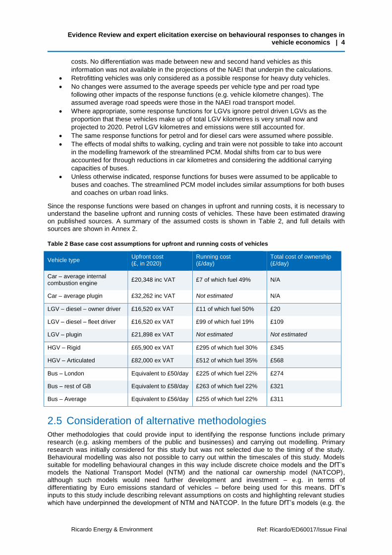
Since the response functions were based on changes in upfront and running costs, it is necessary to understand the baseline upfront and running costs of vehicles. These have been estimated drawing on published sources. A summary of the assumed costs is shown in Table 2, and full details with sources are shown in Annex 2.
Table 2 Base case cost assumptions for upfront and running costs of vehicles
Vehicle type Upfront cost (£, in 2020)
Running cost (£/day)
Total cost of ownership (£/day)
Car – average internal combustion engine
£20,348 inc VAT £7 of which fuel 49% N/A
Car – average plugin £32,262 inc VAT Not estimated N/A
LGV – diesel – owner driver £16,520 ex VAT £11 of which fuel 50% £20
LGV – diesel – fleet driver £16,520 ex VAT £99 of which fuel 19% £109
LGV – plugin £21,898 ex VAT Not estimated Not estimated
HGV – Rigid £65,900 ex VAT £295 of which fuel 30% £345
HGV – Articulated £82,000 ex VAT £512 of which fuel 35% £568
Bus – London Equivalent to £50/day £225 of which fuel 22% £274
Bus – rest of GB Equivalent to £58/day £263 of which fuel 22% £321
Bus – Average Equivalent to £56/day £255 of which fuel 22% £311
2.5 Consideration of alternative methodologies
Other methodologies that could provide input to identifying the response functions include primary research (e.g. asking members of the public and businesses) and carrying out modelling. Primary research was initially considered for this study but was not selected due to the timing of the study. Behavioural modelling was also not possible to carry out within the timescales of this study. Models suitable for modelling behavioural changes in this way include discrete choice models and the DfT’s models the National Transport Model (NTM) and the national car ownership model (NATCOP), although such models would need further development and investment – e.g. in terms of differentiating by Euro emissions standard of vehicles – before being used for this means. DfT’s inputs to this study include describing relevant assumptions on costs and highlighting relevant studies which have underpinned the development of NTM and NATCOP. In the future DfT’s models (e.g. the

Evidence Review and expert elicitation exercise on behavioural responses to changes in vehicle economics | 5
Ricardo Energy & Environment Ref: Ricardo/ED60017/Issue Final
NTM and NATCOP) could be used to identify the possible impacts of policy measures considered by Defra.
3 Limitations
A number of limitations of the approach and of the findings were identified. These are listed together with their implications in Table 3.
Table 3 Limitations and their implications
Limitation Implication
There is a general paucity of published quantified information of the effectiveness of many measures to reduce NO2 and the associated costs and wider benefits of such measures. Many of the response functions are based on very limited evidence.
Modelling and analytical work has to involve a greater number of assumptions and results have a higher degree of uncertainty.
This exercise has based response functions on expert elicitation and literature, but not on primary research or modelling. Some experts from the panel indicated that dynamic modelling may yield valuable likely behavioural responses to cost changes. In particular, models held by the DfT were mentioned by multiple experts as being capable of modelling the outcomes of some of the measures being investigated. It was not possible for the DfT models to be run within the timeframe of the study.
The response functions developed in this study do not reflect the full range of likely impacts and so may under- or overestimate the possible NO2 impacts.
It is recommended that at least DfT’s models (e.g. the NTM and NATCOP) are used to identify the possible impacts of policy measures considered by Defra. These models would need further development and investment before being used for this purpose.
In practice, people and businesses take into account a range of factors in addition to costs of purchasing or running vehicles in their transport behaviour; and that these factors vary for different policy measures. As this exercise didn’t focus on specific transport policy measures, possible responses to these other factors could not be taken into account.
These other factors that would affect people’s/businesses’ behaviours and therefore need to be considered when developing policy options.
Some of the experts on the panel consider that the approach taken in this exercise – i.e. based on upfront or running cost changes of vehicles, and taking a general approach rather than covering specific policy measures – excludes certain measures that in their view have high potential to reduce air pollution. Examples of such measures include low emission strategies within urban areas encompassing a range of specific local measures to reduce demand and smooth traffic flows.
The response functions currently explored should not be interpreted as representing all the possible measures that could be considered.
Traffic levels and their emissions on B roads and smaller local roads can be important in urban areas. The approach taken in the translation tool and streamlined PCM considers emission reductions on major roads only (i.e. motorways and A roads).
The estimated NO2 emissions and concentrations will be underestimates, particularly in urban areas with heavily trafficked roads other than A roads and motorways.
Separate response functions for changes in upfront and running costs for freight and bus operators may not reflect the way that operators evaluate investment opportunities. Many operators evaluate using total cost of ownership.
The estimated responses and hence NO2 emission and concentration impacts may be under- or overestimates.
Insufficient evidence was identified to separate out the effect of independently changing diesel from petrol costs on travel demand. The estimates are based on combined demand for both of these fuels.
It is not possible with this tool to assess the impact on driver behaviour if the price of diesel is varied with respect to petrol.

Evidence Review and expert elicitation exercise on behavioural responses to changes in vehicle economics | 6
Ricardo Energy & Environment Ref: Ricardo/ED60017/Issue Final
Limitation Implication
Predicting actual future behavioural responses across the UK across a varied demographic with variable access to alternative transport modes is not possible.
The response functions should be viewed as providing only a broad indication of what behavioural response on average may occur for a given change in road transport costs.
Whilst the findings have been based on the best available information identified through a literature review and an expert panel, there may still be further literature and evidence that was not identified.
The estimated responses and hence NO2 emission and concentration impacts may be under- or overestimates. Additional response functions may be possible to model.
Future uptake rates of unconventional technologies are particularly uncertain due to market barriers. As the price difference between conventional internal combustion engine and unconventional technologies decreases, uptake of the unconventional technologies may well be slow until price parity (or close to) with conventional vehicles is reached after which uptake rates may accelerate.
The estimated responses and hence NO2 emission and concentration impacts may be under- or overestimates.
Published elasticities – on which many response functions are based – are often only valid over small validity ranges, limited to what magnitude of changes have been observed and analysed. Significant changes in fuel prices for example have occurred but over the medium and long term; no other elements of transport costs (excepting zonal charging) have changed to this extent over a relatively short period.
The validity of each response function is restricted to its own described validity range. Impacts should not be extrapolated beyond the range. In some cases, confidence levels in the response functions may decrease towards the upper ends of validity ranges.
It may take multiple years for the full effects of a policy to change travel behaviour. The impact of a policy in 2020 depends on what the policy is and when the policy came into effect. The response functions have been based where possible on long term (long run) elasticities – however it was not possible to identify long term responses to changes in running costs in restricted zones. The literature is inconclusive as to time periods associated with short run or long run elasticities.
Care should be taken in interpreting the time period over which behavioural responses may occur. The estimated responses and hence NO2 emission and concentration impacts may be overestimated for 2020 if it takes longer for the full behavioural changes to be realised.
Various model-simplifying assumptions had to be made:
• Vehicle markets were assumed to be national.
• No differentiation was made between new and second hand vehicles.
• Retrofitting vehicles was only considered as a possible response for heavy duty vehicles.
• No changes were assumed to the average speeds per vehicle type and per road type following other impacts of the response functions (e.g. vehicle kilometre changes).
• Some response functions for LGVs ignore petrol driven LGVs.
• The same response functions for petrol and for diesel cars were assumed where possible.
• The effects of modal shifts to walking, cycling and train were not possible to take into account. Modal shifts from car to bus were accounted for.
• Most response functions for buses were assumed to be applicable to buses and coaches.
The impact of the assumptions made on the modelling outcomes is considered to be smaller than the uncertainty in the evidence base supporting the levers.
Evidence Review and expert elicitation exercise on behavioural responses to changes in vehicle economics | 7
Ricardo Energy & Environment Ref: Ricardo/ED60017/Issue Final
4 Findings
The main outcome of this exercise is a series of response functions for each vehicle type for input into the ‘Translation Tool’2. The general limitations of the response functions in terms of the approach followed and the outcomes were described in section 3. The response functions and the literature inspected and evidence gathered to support the response functions, and details of the response functions themselves, are described and shown in section 4.3. In addition, a series of findings that help to contextualise the response functions were also identified: these are described in section 4.1.
There was a good degree of consensus among the experts that the response functions represented the best available information identified, and that assumptions made in estimating the response functions were reliable.
4.1 Important considerations for certain sectors
4.1.1 LGVs
It is important to differentiate between different segments of the LGV market when considering changes to running costs. This is because there are different running costs and different perceived running costs. A significant part of LGV usage is not for freight transport but is by the service sector – window cleaners, photocopier repairers etc. In addition, there is a need to distinguish between LGVs driven by employees of large businesses (‘fleet drivers’) and LGVs driven by self-employed workers (‘owner drivers’), because this will affect the perceived running costs.
Owner drivers are unlikely to value their own time when running the vehicle, such that fuel costs become an important part of total running costs. For owner drivers, large increases in daily running costs could significantly impact on net weekly earnings, meaning such businesses would fold or at least would need to find radical alternatives.
For fleet drivers the situation is very different: they perceive higher operating costs, most notably including the driver costs, such that fuel costs are no longer the largest cost. The same £ increase in daily running costs for fleet drivers is a much smaller percentage change than perceived by owner drivers. There may still be a need for significant changes to business practices, including modal shift. Fleet drivers are likely to adopt a total cost of ownership approach (see section 4.1.3 below) when considering their response to changes in their cost base.
In order to distinguish between these LGV types, there is a need to split the total vehicle kilometres attributable to the two types of LGV drivers. Allen & Browne (2010) identified from two DfT surveys (Company Van Survey, 2007 and Survey of Privately-Owned Vans, 2004) that LGV kilometres are split as goods 30%, service trips 25%, commuting 36%, and personal trips 8%. However it is difficult to reliably assign the goods and services between owner drivers and fleet drivers. The DfT Company Van Survey cited by Allen & Browne (2010) shows that in 2005 there were 1.43 million company registered vans out of a total of 3.02 million, i.e. close to 50%. The development of the market in the last decade has seen strong growth in both the owner driver and fleet subsectors (Whiteing, Pers. Comm.), which suggests that a first order assumption on the split in LGV kilometres between the two LGV users can remain at 50%. Appropriate sensitivities of this split range from 75:25 to 25:75.
4.1.2 Plugin vehicles
The market for EV and PHEV LGVs is much less well developed than for cars: there are very few vehicles of this nature on the market at the moment, although this may change in the future (and the extent to which it changes may depend on the level of subsidy or measures to incentivise uptake). This currently small market with potential for substantial expansion leads to higher levels of uncertainty in the possible outcomes.
2 More information on the Streamlined PCM tool and Translation Tool are published at http://uk-air.defra.gov.uk/library/reports?report_id=882
Evidence Review and expert elicitation exercise on behavioural responses to changes in vehicle economics | 8
Ricardo Energy & Environment Ref: Ricardo/ED60017/Issue Final
4.1.3 Total cost of ownership approach
Although response functions have been considered separately for variations in upfront and running costs, freight and bus operators often focus on the payback time of new technologies or alternative fuels and have tight financial margins. Total cost of ownership (TCO) is important and pay-back periods of 3 years are sought by HGVs, longer periods are accepted for buses. Lajunen (2014) shows payback for HEV/EV buses that cost 40% more than conventional is only possible under very particular circumstances even over a 12 year appraisal period.
Both upfront and running costs (including fuel cost changes) influence the TCO; the former is more important for expensive innovative technologies like plug-in hybrid electric (PHEV), electric and hybrids. However, initial upfront cost is still an important consideration in its own right to due to available investment capital. The Cleaner Road Transport Vehicles Regulations 2011 promotes the TCO approach.
4.2 How the response functions could be improved further
First and foremost, it is recognised that the development of the response functions is for a policy screening tool rather than for an in-depth assessment of a single policy. The assessment of how much further the response functions could be improved is considered only within this remit.
For all response functions, and in particular for those response functions which are based on single sources of evidence, additional evidence to support the functions should be identified to increase the confidence in the functions and where possible reduce the uncertainty bounds. Additional evidence could include: further input and review by a wider range of experts, additional literature, primary research or dynamic modelling.
Further evidence could for example enable greater distinction to be made in the response functions between fuel types. Evidence on the cross price elasticities for diesel with respect to petrol would enable the assessment of demand for diesel cars independently from petrol cars and provide for additional policies to be screened.
4.3 Evidence identified and response functions developed
This section is set out as follows:
A reference table outlining where information is located in this section (Table 4)
A series of tables summarising the evidence identified (Tables 5 to 16).
A table describing each response function (Tables 17 to 36).
Table 4 can be used as a contents page for the rest of this section. It indicates, for each vehicle type and cost variable, which tables summarise the evidence identified, and what response functions were developed and where these are described in more detail.
The exercise has found that in some cases a strong evidence base has been identified, for example in the case of relating car usage with fuel (running) costs, with many studies and for which the results of different studies are often quite similar. There are however a number of areas where the evidence is poor, which limits the ability to generate response functions and lowers confidence in any response functions estimated. In some instances this lack of evidence may be because research effort has not focussed on it (e.g. on price differential between two fuels), but in other instances it is because the evidence itself is hard to obtain (e.g. isolating the impacts of congestion charge zones).

Evidence Review and expert elicitation exercise on behavioural responses to changes in vehicle economics | 9
Ricardo Energy & Environment Ref: Ricardo/ED60017/Issue Final
Table 4: Overview of where in this document the evidence is presented and what response functions have been developed and where to find their descriptions.
Vehicle Variable Evidence summary
Response functions developed and where they are described
Cars Upfront Table 5, page 10
Response functions developed for cars
Table 17 Response function 1: Switch from conventionally fuelled Euro 6
cars to Euro 6 PHEVs/BEVs as upfront costs of PHEVs and BEVs decrease (page 31)
Table 18 Response function 3: Reduction in purchase of conventionally fuelled Euro 6 cars as upfront costs of conventionally fuelled cars increase, and limited switch to alternatively fuelled vehicles (hybrids, PHEVs, BEVs) (page 32)
Running Table 6, page 12
Table 19 Response function 12: Changes in car and bus kilometres driven as car running costs change (page 33)
Table 20 Response function 6: Changes in fleet composition due to switches from conventionally to alternatively fuelled Euro 6 cars as running costs of conventionally fuelled cars increases. (page 34)
Running (restricted zones)
Table 7, page 16
Table 21 Response function 13. Changes in car kilometres driven as car running costs in restricted zones change. (page 35)
Table 22 Response function 7. Changes in fleet composition due to switches from conventional to alternative fuelled Euro 6 cars as running costs of conventionally fuelled cars increase in restricted zones (congestion charge). (page 36)
Table 23 Response function 4. Changes in fleet composition, car and bus kilometres as running costs of cars in restricted zones (euro standard based low emission zone) increase. (page 37)
Table 24 Response function 5. Changes in fleet composition, car and bus kilometres as running costs of cars in restricted zones (low emission zone based on zero emission capable cars) increase. (Page 38)
LGVs Upfront Table 7 page 20
Response functions developed for LGVs
Table 25 Response function 2: Switch from Euro 6 diesel LGVs to
PHEVs/BEVs as upfront costs of PHEVs and BEVs decrease (Page
39)
Table 26 Response function 11: Change in LGV kilometres driven as upfront costs of LGVs change (Page 40)
Running Table 9, page 21
Table 27 Response function 10. Change in LGV kilometres driven as LGV running costs change (Page 41)
Table 28 Response function 14. Change in LGV fleet composition due to switch from conventional to alternative fuelled Euro 6 LGVs as running costs of conventionally fuelled LGVs increase (page 42)
Running (restricted zones)
Table 10, page 22
Table 29 Response function 15. Changes in fleet composition, LGV and bus kilometres as running costs of LGVs in restricted zones (euro standard based low emission zone) increase. (page 43)
Table 30 Response function 16. Changes in fleet composition, LGV and bus kilometres as running costs of LGVs in restricted zones (LEZ based on zero emission capable LGVs) increase. (page 44)
HGVs Upfront Table 10 page 24
Response functions developed for HGVs
Table 31 Response function 18: Change in HGV kilometres driven as
upfront costs of HGVs change. (page 45)
Running Table 12, page 25
Table 32 Response function 9: Change in HGV kilometres driven as HGV running costs change. (page 46)
Running (restricted zones)
Table 13, page 26
Table 33 Response function 20: Changes in fleet composition, HGV kilometres and shift to rail as running costs of HGVs in restricted zones
(euro standard based low emission zone) increase. (page 47)
Buses and coaches
Upfront Table 13, page 27
Response functions developed for buses
Table 34 Response function 8: Change in bus kilometres, car kilometres
and passenger rail demand as upfront costs of buses change. (page
48)

Evidence Review and expert elicitation exercise on behavioural responses to changes in vehicle economics | 10
Ricardo Energy & Environment Ref: Ricardo/ED60017/Issue Final
Running Table 15, page 28
Table 35 Response function 19: Change in bus and car kilometres, and passenger rail demand, as bus running costs change. (page 49)
Running (restricted zones)
Table 16, page 30
Table 36 Response function 17. Changes in fleet composition and bus kilometres as running costs of buses in restricted zones (Euro VI based low emission zone) increase (page 50)
4.3.1 Evidence identified for cars
Table 5 Evidence identified and response functions developed for: Cars – upfront costs
Overview
Limited evidence identified in the literature.
The evidence that was available was used to estimate two response functions:
1. Increasing switch from conventionally fuelled Euro 6 cars to Euro 6 PHEVs/BEVs as upfront costs of PHEVs and BEVs decrease.
3. Reduction in purchase of conventionally fuelled Euro 6 cars, and limited switch to alternatively fuelled vehicles (hybrids, PHEVs, BEVs), as upfront costs of conventionally fuelled cars increase.
Evidence identified for impacts of purchase costs on fleet composition, modal shift and on kilometres driven
The DfT’s national car ownership model (NATCOP) includes vehicle purchase price index as one variable affecting car ownership. The impact of changes in car purchase costs on the level of ownership is derived from the ONS household expenditure survey, in which used car purchase makes up one part (around 20-25%) of the weighting as well as newly registered cars. No evidence of any model that translates the change in the price of registering a new car with the average price of all cars on the market. Manufacturers may respond to changes (increases) in purchase price by reducing the margin they expect to make (Worsley, 2015 Pers. Comm.). The DfT has not carried out any project exercise in modelling the sensitivity in NATCOP to changes in new vehicle purchase price, but suggested that changes in upfront cost (in the order of 2% - 20%) will have no significant impact on ownership of cars based on NATCOP methodology (DfT, 2015, Pers. Comm.). DfT have not defined ‘significant’, and it is not clear if it is negligible effect. The effect could potentially be quantified if the NATCOP is run to assess this sensitivity.
The purchase of a second and subsequent cars would be expected to be more price sensitive than the choice of the first/only car. First cars do more mileage and there will be a ‘bounce back’ in that the first car will in some cases substitute for the previously owned second car. So the effect on car km will be perhaps 25% less that the effect on car ownership. And, as noted above, the effect of a new registration tax on the purchase of new cars will be very much less than the same increase in the cost of car ownership as far as total car kilometres are concerned. The effect on fleet composition is likely to be greater but no evidence is available to describe the effect (Worsley, 2015, Pers Comm.).
The current (as at April 2015) grant funding available is up to £5,000 for plugged in cars. Hence within this regime, purchase cost increases [for e.g. conventionally fuelled vehicles] of less than this value might not be sufficient to encourage a shift to PHEVs/BEVs (LowCVP, 2015, Pers. Comm.). A literature review for DfT of ‘what works’ for OLEV (cars only) in terms of adoption and behaviour change was underway in May 2015 led by Brook Lyndhurst.
Various literature have estimated elasticity of car ownership (cars per household) with respect to purchase costs:
o Whelan (2007) estimate -0.34. This is considered to be a reliable estimate as it is used by DfT in NATCOP.
o Goodwin et al. (2004) estimated -0.1 (short run) to -0.2 (long run) from dynamic modelling.
o The literature survey review by Graham and Glaister (2004) cite an estimate by Goodwin (1992) of -0.89. This estimate is discarded as the source material is dated.
o Romilly et al. (1998) estimate -0.29 (short run), -2.19 (long run). This LR estimate appears to be very high and so is discarded. Elasticity estimates by this author for other variables also appear to be higher than other literature.
Eftec (2008) report on a dataset gathered from DVLA which has been used to formulate a model to investigate new car purchases and responses to variations in prices. Regarding purchase costs, the study looks at the impacts on the market if one portion of the vehicles sold are sold at increased prices of +1% (rather than a unilateral increase). The 1% increments in purchase price for single CO2 bands were modelled as leading to changes in purchase decisions, both in terms of purchasers changing which vehicles they purchase, but also in terms of a small proportion of buyers choosing not to purchase
Evidence Review and expert elicitation exercise on behavioural responses to changes in vehicle economics | 11
Ricardo Energy & Environment Ref: Ricardo/ED60017/Issue Final
vehicles. The portion incremented is the cars that fall into a CO2 band e.g. 121-130gCO2/km. Based on the information available in the report, as this perturbation is for a small fraction of sales at any one time, the outcomes are not appropriate to use for the response functions for air emissions. Elasticities with respect to the total market are not presented, however, an elasticity value of -0.5 is implied. However there may be further information from the model underlying this. A separate request was made for DfT to provide this.
LowCVP Buyer Survey participants were unconvinced that additional upfront costs for environmentally friendly cars would be offset by lower running costs (Lane & Banks, 2010, p25). Further perception surveys may be available, but they are not expected to include the elasticities sought.
The Netherlands introduced a series of reforms to its original 42 per cent car purchase tax. From mid-2006, registration taxes were reduced for the most fuel efficient (A- or B-rated) cars. A trial was carried out prior to full implementation of the measure. Evaluation of the trial found that compared to 2001, the market share of the A-labelled cars in 2002 increased from 0.3 to 3.2 per cent, while that of B-labelled cars rose from 9.5 to 16.1 per cent. (Green Fiscal Commission, 2010, p4.)
Sweden introduced a subsidy (approximately €1,000 per car) to encourage consumers to purchase environmentally friendly cars that had emissions below 120g/km (Hennessey and Tol, 2011). However, this subsidy policy had to be removed in 2009, and was replaced with a five year exemption from motor tax, due to a particularly large surge in sales. Lindford and Roxland (2009; cited in Whitehead et al., 2014) estimate that the subsidy in Sweden resulted in a 12% increase in ‘alternatively fuelled vehicle’ sales in 2008. However, looking at data for Stockholm in isolation, it was suggested by this paper that a congestion tax exemption resulted in a 24% increase in alternatively fuelled vehicle sales; double that of the increase from the subsidy. The resulting consumer effect of a congestion tax exemption can vary depending on the distance between where the individual lives and the congestion zone (Whitehead et al., 2014).
An increase in purchase costs of regular fuelled vehicles, combined with likely future incentives for electric vehicles is expected to result in an increased uptake of electric vehicles (Element Energy, Ecolane and University of Aberdeen, 2013 – study for the CCC). Modelling in this study suggests that purchase price reductions of £3,000 per EV to 2020 will be needed to achieve the high UK uptake pathway of vehicles (indicated to be 16% of car and van sales (0.27 million/year) to be EV/PHEV, or a fleet of 0.68 million). This represents a 100% increase in the implied NAEI fleet of EV/PHEV cars and vans. The elasticity cited in this Element study as coming from Eftec (2008) could not be identified. Element Energy et al. (2013, p31) also identified that congestion charge discounts are highly effective in stimulating demand for new vehicle technologies.
Overall data quality assessment
There is little evidence in the identified literature relating purchase cost changes with changes on car use that can be used for the response functions (the focus in literature is usually on fuel price and income).
Non-zero elasticities of car ownership with respect to purchase price are identified in the literature. It may be that the elasticities identified would be expected to play a larger role for larger price changes.
The evidence from the Netherlands whilst interesting is relatively dated and vehicle markets have moved on since then.
Response functions developed
There was sufficient information gathered to estimate two response functions:
1. As upfront costs of PHEVs and BEVs decrease, new car buyers switch purchases from conventionally fuelled Euro 6 cars to Euro 6 PHEVs/BEVs. This function affects fleet composition, but not total kilometres driven. This function is based on the projections in Element Energy et al. (2013) of PHEV/BEV fleet sizes for 2020.
3. As upfront costs of conventionally fuelled Euro 6 cars increase, would-be buyers adopt two behaviours. One is not purchasing vehicles, for which we draw on elasticity estimates from literature relating car ownership to purchase costs. The second is switching purchases to alternatively fuelled vehicles not subject to a price increase, for which we draw on the negative of the elasticity estimates.

Evidence Review and expert elicitation exercise on behavioural responses to changes in vehicle economics | 12
Ricardo Energy & Environment Ref: Ricardo/ED60017/Issue Final
Table 6 Evidence identified and response functions developed for: Cars – running costs
Overview
Limited evidence was identified relating car running cost changes with car fleet composition changes.
There is a wide evidence base of literature estimates of elasticities of car distances driven (vehicle kilometres) with respect to fuel costs or fuel consumption (car running costs). There are also a number of literature estimates of cross-elasticities of bus/rail transport with respect to fuel costs (car running costs).
Very limited evidence was identified for petrol and diesel cross price elasticities.
The evidence that was available was used to estimate two response functions:
12. Changes in car and bus kilometres driven as car running costs change.
6. Changes in fleet composition due to switches from conventional to alternative fuelled Euro 6 cars as running costs of conventionally fuelled cars increases.
Evidence identified for impacts of running costs on fleet composition
Turcksin & Macharis (Not Dated) undertook a survey of drivers in Belgium (around 1,700 respondents in total) to investigate the potential impacts of a range of policy measures on purchase decisions. The policies considered were (1) a kilometre charge, (2) a congestion charge, (3) an increasing parking tariff and (4) an extra pollution tax. Respondents were asked to state at which price they would consider the purchase of a cleaner car. The results generated buy-response curves – showing the cumulative proportion (%) of people that would consider the purchase of a cleaner car at each price change bracket.
The 2002 company car taxation reforms played a major part in shifting the composition of the fleet from petrol to diesel pretty swiftly (Stephen Potter, Pers. Comm. 2015; HMRC, 2006). The choice of company car is significantly affected by the costs of CO2 banded company car tax and NIC.
UK motorists are taking account of fuel economy and shifting towards smaller more fuel-efficient cars, or diesel cars (Lane & Banks, 2010).
Brand et al (2013, p.135) identify that annual costs would have to increase by at least £1100 (2004 prices) before (in the short term) consumers would switch to an alternative fuel or a smaller engine. In the longer term increases in running costs would be expected to affect new car choice, perhaps in line with recent trends, with a shift to more efficient cars offset in part by increasing income related demand for larger vehicles. 33% of a survey’s respondents would buy another vehicle if VED differential was £60 (at 2009 prices) rising to 55% for a £180 differential. The highest difference offered in the survey was £360 at which point 28% would not switch, rising to 40% for those owning larger vehicles. (Brand et al. 2013, p135)
If, for example, VED was changed to encourage a shift away from diesel, the second hand price of diesel cars would fall and of petrol cars would rise, offsetting to a considerable extent the intended effect of the VED change over the short to medium term. The DfT used to have a car market model which incorporated such responses, but the model is no longer maintained or used (Worsley, 2015, Pers. Comm.)
Higher purchase costs, running costs and costs in restricted zones is likely to result in an increased shift towards electric vehicles (Element Energy, Ecolane and University of Aberdeen 2013).
The demand for car parks and parking facilities can be reduced as a result of an increase in driving costs (Litman, 2013).
Evidence identified for impacts of running costs on vehicle kilometres
Elasticities presented here are on fuel costs, i.e. changes in km driven due to changes in the cost per km of driving. Elasticities of fuel demand, i.e. changes in fuel demand with respect to changes in the pump price, are covered in the subsequent table.
Impact of changes of car running costs on car use
Estimates of long run elasticity of car use (vehicle km) with respect to fuel cost from literature:
-0.3 (range -0.25 to -0.35) (DfT 2014a, p48).
-0.1 to -0.5, with values of up to -0.79 reported (p14). Urban specific elasticity of -0.2 (RAND Europe 2014).
-0.29 to -0.31 (Goodwin et al 2011)
-0.26, -0.31 (Graham and Glaister, 2004)
-0.15 (Godwin, 1992, cited in Litman, 2013)
Evidence Review and expert elicitation exercise on behavioural responses to changes in vehicle economics | 13
Ricardo Energy & Environment Ref: Ricardo/ED60017/Issue Final
-0.29 (TRACE, 1999, cited in Litman, 2013)
-0.26 (Schimek, 1997; cited in Turcksin and Macharis, undated).
-0.197 (Hensher, 1997, cited in Litman, 2013)
Estimates of short run elasticity of car use (vehicle km) with respect to fuel cost from literature:
–0.16 (Graham and Glaister (2004) cite de Jong and Gunn (2001)). Plus based on fuel price elasticity for car trips they find that the immediate consumer response to a fuel price change is to modify the number of trips made, but over time they make even more substantial changes to the distance travelled.
-0.4 (Green Fiscal Commission, 2010, p6, citing Glaister and Graham 2000, and Goodwin 2002)
The elasticity of car use (vkm) with respect to index of total motoring costs of -1.94 identified by Romilly et al 2001 has been discarded due to perception of two peer reviewers that the value is a very high estimate.
These elasticities may reduce by half for price changes towards the upper end of the range considered in this study (Worsley, 2015 Pers. Comm.).
Rebound effects should result in lower long run fuel price elasticities. Two rebounds occur – a shift to more fuel efficient vehicles, and an increase in road traffic because the cost of driving has fallen.
Li et al., (2009; cited in Hennessey and Tol, 2011) found that a 0.22% increase in car fleet economy could be achieved in the short term, and a 2.04% increase in the long term, with a 10% increase in fuel prices.
Many of the above cited elasticities are summarised in Litman (2013).
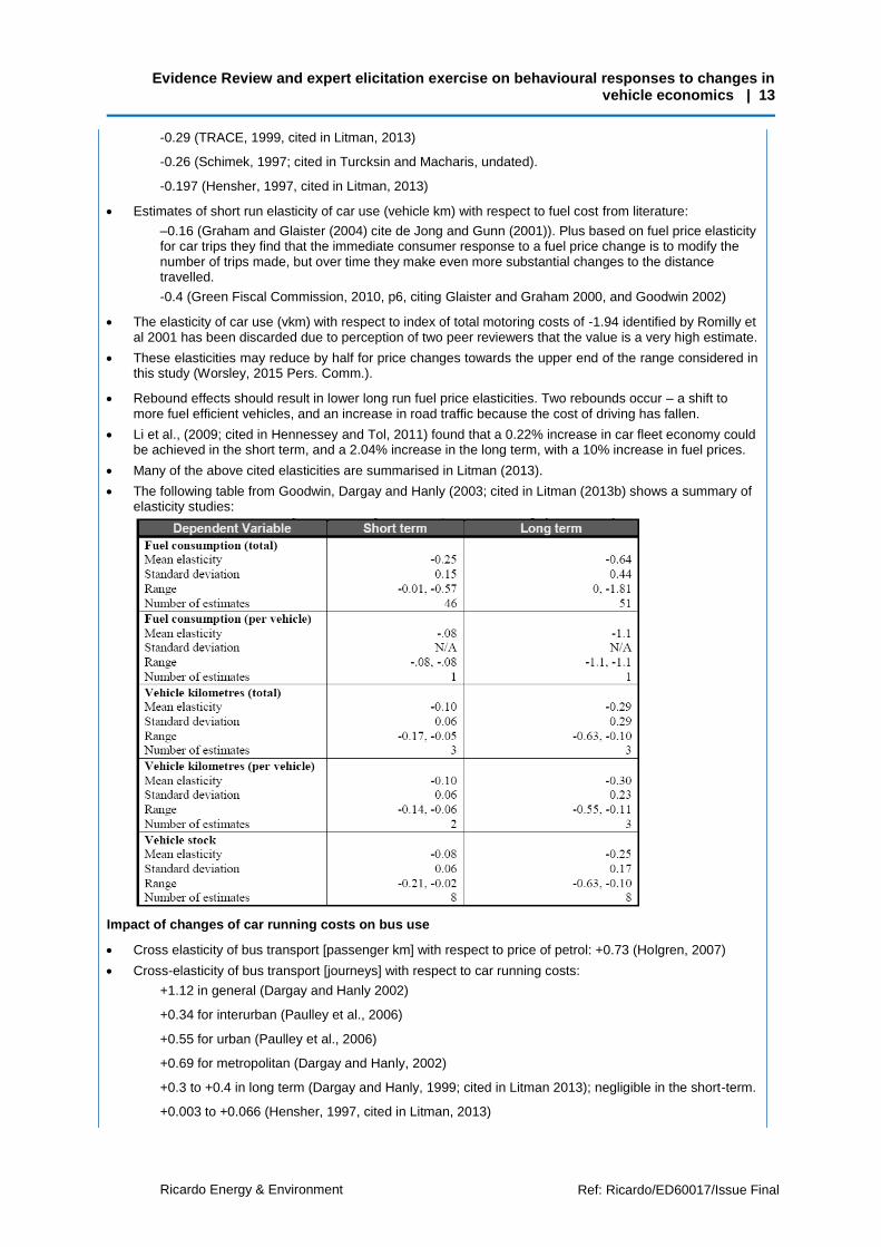
The following table from Goodwin, Dargay and Hanly (2003; cited in Litman (2013b) shows a summary of elasticity studies:
Impact of changes of car running costs on bus use
Cross elasticity of bus transport [passenger km] with respect to price of petrol: +0.73 (Holgren, 2007)
Cross-elasticity of bus transport [journeys] with respect to car running costs:
+1.12 in general (Dargay and Hanly 2002)
+0.34 for interurban (Paulley et al., 2006)
+0.55 for urban (Paulley et al., 2006)
+0.69 for metropolitan (Dargay and Hanly, 2002)
+0.3 to +0.4 in long term (Dargay and Hanly, 1999; cited in Litman 2013); negligible in the short-term.
+0.003 to +0.066 (Hensher, 1997, cited in Litman, 2013)

Evidence Review and expert elicitation exercise on behavioural responses to changes in vehicle economics | 14
Ricardo Energy & Environment Ref: Ricardo/ED60017/Issue Final
Litman (2008) cite TRACE (1999) with elasticity of public transport with respect to fuel price as +0.14
A paper on this topic by Acutt and Dodgson (1996) has been discarded as the car fleet has almost entirely turned over since then.
No adjustment is required to passenger-bus-trip or bus-passenger-kilometre elasticities with respect to fares in order to use the elasticities as bus-vehicle-kilometres with respect to fares – as a first approximation these are likely to be similar (Maddison, 2015, Pers. Comm.). However, the alternative view is that bus loadings will change but not necessarily vehicle kilometres to the same degree.
Impact of changes of car running costs on rail use
Cross elasticity of rail transport [journeys] with respect to car running costs:
+0.25 interurban (Paulley et al 2006)
+0.59 for urban (Paulley et al 2006), although lower than this for trips in the London Travelcard area (Worsley, 2015, Pers. Comm.)
zero for commuting from the rest of South East to London (Worsley, 2015, Pers. Comm.)
+0.003 to +0.053 (Hensher, 1997, cited in Litman, 2013)
Brand et al. (2012) modelled that passenger car demand compared to a baseline projection would be 3% lower in 2020 and 4% lower in 2050. This is because of 7% higher costs in using a car in 2020 and 8% higher costs in 2050 (using a fuel duty scenario). This paper suggests that this would not encourage a shift towards public transport, and instead would simply result in an overall decrease in domestic travel.
Evidence identified for cross elasticities between petrol and diesel
Petrol own price elasticities in the literature: -0.34 to -0.38 (Dahl 2012; Polemis 2006)
Petrol long run cross elasticity with respect to diesel price: +0.10 (Polemis 2006) [i.e. an increase in the price of diesel of 100% would lead to an increase in demand for petrol of 10%]. The Polemis 2006 study is derived solely from Greece which has a subsidised diesel tax so the differential cost is far greater than the UK, and the incentives for adoption on fuel price grounds greater. The decision to choose diesel on price ground in the UK is more marginal given the per-litre cost is higher (unless other cost of use factors such as VED and company car taxation are brought in). Therefore this elasticity value may have applicability limitations given that diesel in Greece is both lower price and more energy efficient whereas in the UK it is higher price and more energy efficient. The wider tax context would tend to keep it competitive despite a fuel cost increase as fuel cost was not the primary motivation in the first place.
Diesel own price elasticities: -0.16 to -0.30 (Dahl 2012; Ramli and Graham, 2014)
A PhD thesis by Al Dossary from University of Colorado was identified that may provide more evidence on cross-price elasticities. Although the thesis was requested, it was not made available.
Eftec (2008) carried out a modelling exercise on incrementing the diesel price by up to 10% and identifies shifts in car purchase behaviour. The Eftec paper estimates in general some switching to petrol vehicles, but also shifts in terms of reductions in vehicles purchased. The implied elasticity of purchase of all vehicles with respect to fuel price (elasticities were not presented in the report) are -0.26 for a 1% diesel price increment declining to -0.22 for a 10% diesel increment. However no information was available in the Eftec paper as to what the resulting split between diesel and petrol cars is, nor on cross price elasticities.
Overall data quality assessment
On fleet composition impacts evidence:
The original surveys underpinning the Brand et al (2013) are now quite outdated. The surveys were performed when graduated VED was first introduced – it is possible that consumer perceptions and preferences changed. It is also unclear from Brand et al (2013) what the longer term responses (price point at which behaviours switch) might be if these were short term responses. Owner responses are likely to be more complex than switching at specific price points: e.g. following elasticities, or S-shaped response curves (e.g. low uptake at small cost differences, then accelerated and flatten off – to allow for early and late adopters).
On vehicle kilometres impacts evidence:
There is a substantial evidence base in the literature on elasticity of car km travelled with respect to fuel costs. These estimates are mostly in agreement with each other; one or two estimates are discarded as being anomalous.
Greater emphasis in literature on own price elasticities rather than cross price elasticities.

Evidence Review and expert elicitation exercise on behavioural responses to changes in vehicle economics | 15
Ricardo Energy & Environment Ref: Ricardo/ED60017/Issue Final
Elasticity validity range is maximum 40-50% change from existing costs (this is still high as 50% change in fuel costs has not been experienced). Beyond this range, not clear what behavioural changes may occur.
The cross elasticities of bus transport identified in the literature appeared high to the peer reviewers:
o These elasticities look high because around a third of all passengers travel on concessionary fares, and for whom car is an option only for a small number, and because some 45% of all bus trips are in London, where car use is much lower than average.
o If these scales of elasticity were to be realised across the UK public transport network then it implies a lot more buses in particular, running on new routes at a wider range of times, therefore in less efficient times and places. Therefore ‘achieving’ the elasticity would have a disproportionate impact on public transport vehicle-km. The additional capacity may be commensurate with a rise in the viability of flexible transport services operated by smaller vehicles, which would to some extent offset this effect. However, public transport fares may rise to maintain profitability/viability, which may suppress travel so not all the predicted trips would emerge.
o The full effects of these elasticities are likely to be very long-run, relying on behavioural change such as residential relocation to be nearer public transport.
Due to substantial variation across the UK in bus travel and demand, elasticity ranges need to reflect this variation.
On petrol / diesel cross elasticities:
Own price elasticities have been estimated, but these have been derived in situations where petrol and diesel were changing in similar ways.
Only one information source on cross price elasticities for petrol, but this estimate is not considered applicable to the UK situation (reasons described above).
No identified literature with published cross price elasticities for diesel. One study for DfT (Eftec, 2008) investigated the impacts on purchase of diesel vehicles when diesel prices rise, however the study did not include information on the split of petrol and diesel. Further information was requested from DfT on the data underpinning the Eftec (2008) study but not provided.
Response functions developed
There was sufficient information gathered to estimate two response functions:
12. As running costs of all cars change, car kilometres driven are estimated from fuel cost elasticities. The range of elasticities identified in the literature have been represented with a central value of -0.3 and low/high bounds of -0.2/-0.4 respectively. The modal switch to bus is also estimated from the cross-elasticities of bus transport with respect to car running costs identified in the literature.
6. As running costs of conventionally fuelled cars increases, the impacts of switches in purchase decisions from conventional to alternative fuelled Euro 6 cars on fleet composition are estimated. This is based on Turcksin & Macharis (undated).

Evidence Review and expert elicitation exercise on behavioural responses to changes in vehicle economics | 16
Ricardo Energy & Environment Ref: Ricardo/ED60017/Issue Final
Table 7 Evidence identified and response functions developed for: Cars – running costs in restricted zones
Overview
Some evidence was identified on the impact of parking charges on car demand. However, price elasticities of parking are very specific to the context they are reported. These elasticity estimates have not been used to inform response functions.
Evidence is identified on elasticities related to congestion charge schemes, although these range widely for single schemes. No publication is identified that assembles observations on many congestion charges and changes in transport demand to derive elasticities. The literature indicates that congestion charge elasticities should not be translated to other years or other general costs or congestion charge changes. Hence there is large uncertainty in using such information.
Very limited information was identified on low emission zones impacts on fleet composition and vehicle kilometres.
There was sufficient information gathered to estimate four response functions:
13. Changes in car kilometres driven as car running costs in restricted zones change.
7. Changes in fleet composition due to switches from conventional to alternative fuelled Euro 6 cars as running costs of conventionally fuelled cars increase in restricted zones (congestion charge).
4. Changes in fleet composition, car and bus kilometres as running costs of cars in restricted zones (euro standard based low emission zone) increase.
5. Changes in fleet composition, car and bus kilometres as running costs of cars in restricted zones (low emission zone based on zero emission capable cars) increase.
Evidence identified for impacts of running costs on fleet composition, modal shift and on kilometres driven in restricted zones
Parking prices
Tipping points on modal shift as well as fuel switch without modal shift are not a matter of a graded shift in daily running costs. These are about the costs and choices that occur at decision points. It is also a matter of relative costs to the options concerned. So for short-term decision making, parking costs at a workplace plus any tolls involved are relative to perceived fuel costs. Capital and maintenance costs, annual taxation etc. play no part in the decision. (Stephen Potter, 2015 Pers. Comm.)
Elasticity of demand for private transport with respect to the price of parking:
-0.31 to -0.32 Feeney (1989)
-0.30 Marsden (2006)
-0.13 at £0.80/day (2014 prices), -1.00 at £4.01/day, -2.40 at £7.21/day, -6.22 at £15.23/day Balcombe et al. (2004), citing Clark and Allsop (1993).
-0.07 Turcksin and Macharis (undated) citing TRACE (1999)
Typically -0.1 to -0.3 for vehicle trips in the US (TRL, 2010)
The applicability to the present day of above elasticities estimated in the 1980s and 1990s is limited.
Values are likely to differ by urban area, and values may be smaller in London where parking is very limited (as well as expensive). (Worsley, 2015, Pers. Comm.)
The provision of free workplace parking has a significant impact on the modal choice of affected commuters (Feeney 1989, Marsden 2006) but not all car travellers. A significant application of this policy might be expected to free up road space for other travellers who may not be seeking to park in the affected zone. This has been observed in cities which introduced restraint parking policies but saw travel levels remain stubbornly high e.g. Oxford for 3 decades of progressive parking policy, with no reduction in traffic until through traffic restrictions also implemented. Clearly this is partly due to route choice, but at the margin there will be people who choose to use public transport in part as a result of traffic conditions, and switch to segregated public transport when congestion rises (Parkhurst, 2015, Pers. Comm.).
TRL (2010) also find the following
o de Jong & Gunn (2001) is a key meta-analysis study on parking elasticities of demand
o elasticities of -1.8 for congestion tolls in the US and -1.2 for parking fees (based on a 2006 US paper)
o elasticity of parking demand based on various parking taxes typically in the range –0.2 to –0.4
Evidence Review and expert elicitation exercise on behavioural responses to changes in vehicle economics | 17
Ricardo Energy & Environment Ref: Ricardo/ED60017/Issue Final
o price elasticities of parking have ranges that vary greatly – by time, location etc – and therefore must be interpreted within the context they are reported.
o information on long-run elasticities is lacking as few time-series analyses have been undertaken.
Parking charges have a greater impact than fuel price on vehicle trips: a $1 parking fee would have the same effect in reducing vehicle travel as an increase in fuel price of between $1.50 and $2.00 per trip (US EPA, 1998; cited in Litman, 2013).
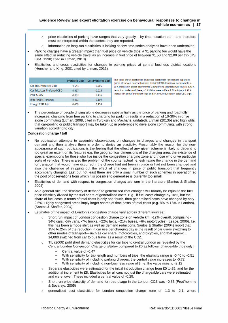
Elasticities and cross elasticities for changes in parking prices at central business district locations (Hensher and King, 2001 cited by Litman, 2013):
The percentage of people driving alone decreases substantially as the price of parking and road tolls increases: changing from free parking to charging for parking results in a reduction of 10-30% in drive alone commuting (Litman, 2008, cited in Turcksin and Macharis, undated). Litman (2013b) also highlights that car-pooling or public transport may be taken up in preference to drive alone commuting, with strong variation according to city.
Congestion charge / toll
No publication attempts to assemble observations on changes in charges and changes in transport demand and then analyse them in order to derive an elasticity. Presumably the reason for the non-appearance of such publications is the feeling that the effect of any given scheme is likely to depend to too great an extent on its features e.g. the geographical dimensions of the charging area, the existence of special exemptions for those who live inside the congestion charging zone and those who drive particular sorts of vehicles. There is also the problem of the counterfactual i.e. estimating the change in the demand for transport that would have occurred if the charge had not been in place or had not been changed and also the challenge of stripping out the effect of changes in price of public transport that frequently accompany charging. Last but not least there are only a small number of such schemes in operation so the pool of observations from which it is possible to generalise is currently too small.
Elasticities of demand with respect to congestion charges are rare in the literature (Santos & Shaffer, 2004)
As a general rule, the sensitivity of demand to generalised cost changes will broadly be equal to the fuel price elasticity divided by the fuel share of generalised costs. E.g., if fuel costs change by 10%, but the share of fuel costs in terms of total costs is only one fourth, then generalised costs have changed by only 2.5%. Highly congested areas imply larger shares of time costs of total costs (e.g. 8% to 16% in London). (Santos & Shaffer, 2004)
Estimates of the impact of London’s congestion charge vary across different sources:
o Short run impact of London congestion charge zone on vehicle km: -12% overall, comprising -34% cars, -5% vans, -7% trucks, +22% taxis, +21% buses, +6% motorcycles) (Leape, 2006). I.e. this has been a mode shift as well as demand reductions. Santos & Shaffer (2004) report that 15% to 25% of the reduction in car use per charging day is the result of car users switching to other modes of transport—such as car share, motorcycles, and bicycles, and that approx.. 14,000 switched from car to bus travel as a result of the CCZ.
o TfL (2008) published demand elasticities for car trips to central London as revealed by the Central London Congestion Charge of £8/day compared to £0 as follows [chargeable trips only]:
Central value of -0.47 With sensitivity for trip length and numbers of trips, the elasticity range is -0.40 to -0.51 With sensitivity of including parking charges, the central value increases to -0.72 With sensitivity of including non-business value of time, the value rises to -2.12
o Separate elasticities were estimated for the initial introduction change from £0 to £5, and for the additional increment to £8. Elasticities for all cars not just the chargeable cars were estimated and were lower. These included a central value of -0.29.
o Short run price elasticity of demand for road usage in the London CCZ was –0.83 (Prud’homme & Bocarejo, 2005)
o generalised cost elasticities for London congestion charge zone of -1.3 to -2.1, where
Evidence Review and expert elicitation exercise on behavioural responses to changes in vehicle economics | 18
Ricardo Energy & Environment Ref: Ricardo/ED60017/Issue Final
generalised costs include all (amortised) capital and running costs of vehicles and the value of time (Santos and Shaffer, 2004). London would expect to have higher elasticities of demand for travel by car than in other areas due to its higher provision of public transport alternatives. (Santos and Shaffer, 2004).
o Santos and Fraser (2006) find that:
The generalised cost elasticity of demand for trips gives a measure of the sensitivity of drivers’ response when deciding on the number of trips when the generalised cost of those trips changes. General cost elasticity of demand for trips: −0.96 for cars.
elasticities of demand of −0.27 for cars, for the increment from £0 to £5
elasticities were lower for the increment from £5 to £8, between −0.03 and −0.10.
congestion charge elasticities should not be translated to other years or other general costs or congestion charge changes.
o Bowen (2010) found elasticities of –0.197, –0.06, and –0.169 of cars entering the charging zone with respect to the congestion charge increments of £0-£5 and a £5 - £8 charge for the original zone, and a £0- £8 charge for the Western Extension Zone respectively.
In a Leicester trial of a toll, on average, 2% of participants changed from car to bus, 15% changed from car to park and ride, 25% changed route, and 13% changed travel time. The price of the toll also affected results: at a toll of £2 to £3, 18% of participants changed route, and this increased to 38% when the toll was increased to £10. However, peer review comments on this Leicester study suggest that the willingness to pay results may have been over-stated due to study design.
A meta-analysis of point elasticities for Singapore congestion zone gives -0.12 to -0.35 (Santos & Shaffer, 2004). Turcksin and Macharis (undated) find the Singapore toll elasticity to range from -0.19 to -0.58.
The Stockholm congestion charge was introduced in 2006. The tax is applied each time a vehicle enters or exits the congestion tax area and has a variable pricing system depending on the time of day. The maximum charge is currently 60 SEK (approximately £4.50) per day. For the Stockholm congestion tax, Whitehead et al. (2014) state that:
o The exemption substantially increased the share of newly purchased, private, exempt energy
efficient vehicles (EEVs) in Stockholm by 1.8% (±0.3%; 95% C.I.) to a total share of 18.8%.
However, a subsidy scheme was also introduced in 2008 which would have also contributed to
the increase of EEVs.
o This increase in demand saw an additional 519 (±91; 95% C.I.) new exempt EEVs purchased in
Stockholm during 2008, equivalent to a 10.7% increase in private sales. This estimate is
consistent with existing literature on the subject.
o A much larger effect was found for those commuting across the congestion tax area. A 13%
increase in EEV private sales is stated for those living inside the congestion charging area,
compared with a 5% increase in exempt EEV sales for those living outside the zone.
The median toll elasticity for New York is -0.10 for cars (Hirschman et al., 1995, cited in Turcksin and Macharis, undated)
Norwegian toll roads had an elasticity of approximately -0.45 (Odeck and Brathan, 2008; cited in Turcksin and Macharis, undated).
The difference between flat-rate tolls and variable tolls (e.g. those where the cost changes according to time or congestion level) was examined by Burris (2003’ cited in Turcksin and Macharis, n.d). They found that a flat-rate toll had an elasticity is -0.03 to -0.35 compared to the variable toll which had an elasticity of -0.16 to -1.0
Spears, Boarnet and Handy (2010; cited in Litman, 2013) estimate that a 10% increase in toll price would reduce the traffic frequenting that road by 1.0% to 4.5%; an elasticity of -0.1 to -0.45. Also in Litman (2013), O’Mahony, Geraghty and Humphreys (2000) concluded that a €6.40 congestion fee would reduce total trips by 5.7%, but peak period trips by 21.6%.
Under the hypothetical scenarios of a doubling in fuel prices or a rebate for EEVs, there would be little effect on the share of these vehicles in Texas, USA (Musti and Kockelman, 2011, cited by Whitehead et al. 2014). However, implementing a ‘fee-bate’ system would increase the share of EEVs by approximately 10%.
May and Milne (2000; cited in Turcksin and Macharis, undated) compare the different fee needed to reduce trips by 10% across different types of road pricing. They find the following are equivalent (values in original year of currency): £0.45/crossing for cordon pricing, £0.20/km for distance-based pricing, £0.11/minute for time-based pricing, and £2.00/min delay for congestion pricing.
Increasing mileage based fees lead to further travel reductions (Deakin & Harvey, 1997, cited by Victoria Transport Policy Institute, 2014): $0.01/mile leads to 1.8% travel reduction, rising to $0.10/mile leads to 15.2% travel reduction (2001 US$).

Evidence Review and expert elicitation exercise on behavioural responses to changes in vehicle economics | 19
Ricardo Energy & Environment Ref: Ricardo/ED60017/Issue Final
Low emission zones
Estimates for the impact of the ULEZ in London, with £12.50 charge (TfL, pers. Comm.).
o 73% of cars would be unaffected as already compliant
o 18% of cars would invest to become compliant
o 2% of cars would pay the charge
o 2% would not travel (reduction in vkm)
o 3% would change mode
o 3% would change route (increase in vkm)
o Overall -5% vkm in central zone, -1% on the inner ring road (IRR) and in inner London, and no change in Outer London. The implied elasticity is around -0.09 assuming fuel costs of £10/day, dropping to -0.07 for fuel costs of £5/day.
Further discussions with TfL regarding their modelling of the ULEZ for London highlighted that:
o TfL adopted the elasticity for chargeable cars of -0.47 over charge ranges up to £20-25/day. The elasticity value would not be applicable at higher charges, and instead an exponential response would be expected at higher charges
o The -0.47 value applies only to the cars to which the charge applied. With respect to all vehicles, the value -0.29 applies. Any back-calculated elasticities from the ULEZ modelling vkm outputs would be elasticities for all vehicles, not just chargeable ones.
o Elasticities with respect to trips in the CCZ or ULEZ were used interchangeably as if they were with respect to vkm.
Ricardo Energy & Environment has derived response curves for each Euro standard from the information TfL have provided on the ULEZ. These response curves are specific to the London ULEZ and its design around Euro 6 diesel and Euro 4 petrol standards.
Overall data quality assessment
Price elasticities of parking must be interpreted within the context they are reported. It is difficult to therefore extrapolate a UK national estimate from the literature on parking elasticities.
No publication attempts to assemble observations on congestion charges and changes in transport demand to derive elasticities. Although evidence exists on the change in the demand for particular forms of transport in areas where charges are in operation, this information is too specific in order to enable researchers to combine such findings in order to make simplistic / generalised statements about the effect of a proposed charge elsewhere.
The literature indicates that congestion charge elasticities should not be translated to other years or other general costs or congestion charge changes. As such we resort to using wide range of elasticities.
Very limited information was identified on low emission zones impacts on fleet composition and vehicle kilometres. The fleet propensity to switch vehicles in London for compliance purposes may be different to other parts of the country. There is uncertainty around the impacts of low emission zones in areas that are not already subject to a congestion charge and which have fewer public transport alternatives than in London.
Response functions developed
There was sufficient information gathered to estimate four response functions:
13. As running costs of all cars in restricted zones increase, car kilometres driven within restricted zones are estimated using elasticities to decrease. The range of elasticities identified in the literature have been represented with a central value of -0.29 and low/high bounds of -0.07/-0.45 respectively.
7. As running costs of conventional cars driven in restricted zones increase, the impacts of switches in purchase decisions from conventional to alternative fuelled Euro 6 cars on fleet composition are estimated. This is based on Turcksin & Macharis (undated) on congestion charges.
4. As running costs of cars in restricted zones increase, the impacts on car kilometres, shifts to compliant vehicles and modal shift to bus are estimated. This draws on estimates by TfL for a low emission zone based on Euro 4 petrol and Euro 6 diesel.
5. As running costs of cars in restricted zones increase, the impacts on car kilometres, shifts to compliant vehicles and modal shift to bus are estimated. This draws on estimates by TfL for a low emission zone based on zero emission capable (ZEC) cars.
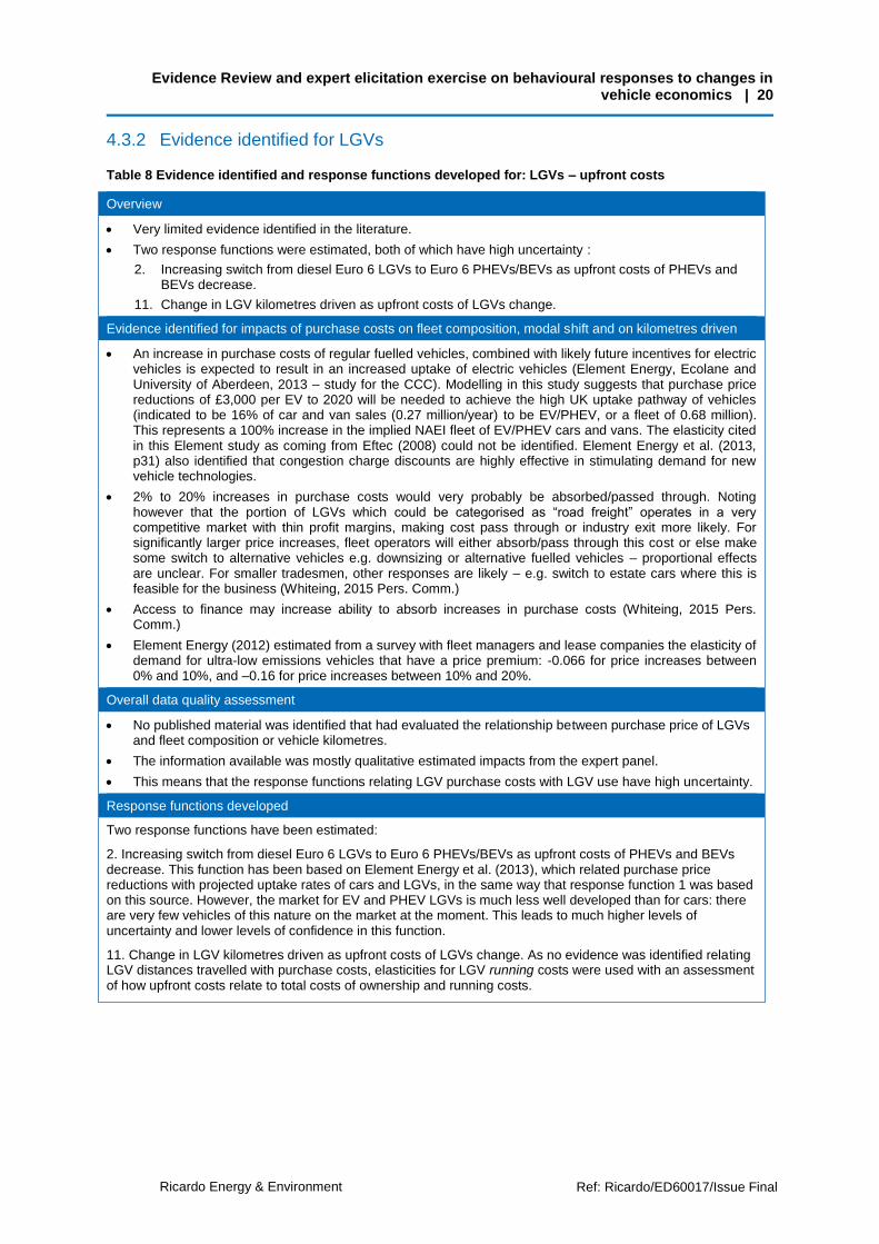
Evidence Review and expert elicitation exercise on behavioural responses to changes in vehicle economics | 20
Ricardo Energy & Environment Ref: Ricardo/ED60017/Issue Final
4.3.2 Evidence identified for LGVs
Table 8 Evidence identified and response functions developed for: LGVs – upfront costs
Overview
Very limited evidence identified in the literature.
Two response functions were estimated, both of which have high uncertainty :
2. Increasing switch from diesel Euro 6 LGVs to Euro 6 PHEVs/BEVs as upfront costs of PHEVs and BEVs decrease.
11. Change in LGV kilometres driven as upfront costs of LGVs change.
Evidence identified for impacts of purchase costs on fleet composition, modal shift and on kilometres driven
An increase in purchase costs of regular fuelled vehicles, combined with likely future incentives for electric vehicles is expected to result in an increased uptake of electric vehicles (Element Energy, Ecolane and University of Aberdeen, 2013 – study for the CCC). Modelling in this study suggests that purchase price reductions of £3,000 per EV to 2020 will be needed to achieve the high UK uptake pathway of vehicles (indicated to be 16% of car and van sales (0.27 million/year) to be EV/PHEV, or a fleet of 0.68 million). This represents a 100% increase in the implied NAEI fleet of EV/PHEV cars and vans. The elasticity cited in this Element study as coming from Eftec (2008) could not be identified. Element Energy et al. (2013, p31) also identified that congestion charge discounts are highly effective in stimulating demand for new vehicle technologies.
2% to 20% increases in purchase costs would very probably be absorbed/passed through. Noting however that the portion of LGVs which could be categorised as “road freight” operates in a very competitive market with thin profit margins, making cost pass through or industry exit more likely. For significantly larger price increases, fleet operators will either absorb/pass through this cost or else make some switch to alternative vehicles e.g. downsizing or alternative fuelled vehicles – proportional effects are unclear. For smaller tradesmen, other responses are likely – e.g. switch to estate cars where this is feasible for the business (Whiteing, 2015 Pers. Comm.)
Access to finance may increase ability to absorb increases in purchase costs (Whiteing, 2015 Pers. Comm.)
Element Energy (2012) estimated from a survey with fleet managers and lease companies the elasticity of demand for ultra-low emissions vehicles that have a price premium: -0.066 for price increases between 0% and 10%, and –0.16 for price increases between 10% and 20%.
Overall data quality assessment
No published material was identified that had evaluated the relationship between purchase price of LGVs and fleet composition or vehicle kilometres.
The information available was mostly qualitative estimated impacts from the expert panel.
This means that the response functions relating LGV purchase costs with LGV use have high uncertainty.
Response functions developed
Two response functions have been estimated:
2. Increasing switch from diesel Euro 6 LGVs to Euro 6 PHEVs/BEVs as upfront costs of PHEVs and BEVs decrease. This function has been based on Element Energy et al. (2013), which related purchase price reductions with projected uptake rates of cars and LGVs, in the same way that response function 1 was based on this source. However, the market for EV and PHEV LGVs is much less well developed than for cars: there are very few vehicles of this nature on the market at the moment. This leads to much higher levels of uncertainty and lower levels of confidence in this function.
11. Change in LGV kilometres driven as upfront costs of LGVs change. As no evidence was identified relating LGV distances travelled with purchase costs, elasticities for LGV running costs were used with an assessment of how upfront costs relate to total costs of ownership and running costs.

Evidence Review and expert elicitation exercise on behavioural responses to changes in vehicle economics | 21
Ricardo Energy & Environment Ref: Ricardo/ED60017/Issue Final
Table 9 Evidence identified and response functions developed for: LGVs – running costs
Overview
Very limited evidence identified relating LGV running costs to fleet composition or vehicle kilometres.
LGVs need to be separated into two types: owner drivers and fleet drivers.
Two response functions were estimated:
10. Changes in LGV kilometres driven as LGV running costs change.
14. Changes in fleet composition of Euro 6 LGVs due to switches from conventional to alternative fuelled Euro 6 LGVs as running costs of conventionally fuelled LGVs increase.
Evidence identified for impacts of running costs on fleet composition and vehicle kilometres
Expect similarly low values for LGV elasticities with respect to fuel prices as for private motoring, given the difficulty of substitution in many situations, and the similarity of car commuting to van use. The accepted values for cars (-0.3) would be an appropriate starting point, but are likely to be lower than this (Whiteing, 2015, Pers. Comm.).
Need to split LGV users into (Whiteing, 2015, Pers. Comm.):
o Owner-drivers - self-employed, e.g. in services, for whom running costs consist of perceived fuel costs only.
o Fleet LGVs driven by employees of larger companies, e.g. delivery companies, for whom running costs include fuel, time cost of driver and vehicle maintenance.
For the first type of LGV user, £2/day increase on top of perceived daily fuel costs of £5 to £10 (i.e. 40% to 20%) is small but would reduce vkm by 6-12% using the -0.3 elasticity. An additional £100/day is however off the scale considering average weekly earnings; vkm would reduce to zero (cease trading) well before reaching £100/day for these LGV users. Tipping point is not far up the scale. Tradesmen would restrict market size to minimise travel, potentially impacting on prices of goods/services.
For the second type of LGV user, £2/day cost is easily absorbable. £100/day increase might double daily running cost, reducing vkm by 30%. In fact such changes (with low margin business meaning cost pass through) may force a resurgence in a wider range of commercial vehicles and travelling practices. E.g. parcel delivery businesses switching to consolidated “click/collect” systems rather than home delivery, which would be consistent with strong mileage reductions.
We are already seeing a rise in cycle freight deliveries. Internationally and in the UK in the past businesses survived with a much lower reliance on motorised LGVs. Public transport could be used for some journeys. Businesses would need to offer a flexible response to travel and reorganise business. If market areas shrank then competition would fall, so there would potentially be more clients served in the reduced area and with the potential for prices to rise to cover higher costs (Parkhurst, 2015, Pers. Comm.).
Santos and Fraser (2006) find that the general cost elasticity of demand for trips is −0.53 for LGVs (note this includes a valuation of time).
Overall data quality assessment
Very little evidence identified in the literature on LGVs and demand elasticities.
Much of the evidence identified is qualitative estimations of impacts from the expert panel.
Response functions developed
Two response functions have been estimated:
10. As running costs of all LGVs change, LGV kilometres driven are estimated using fuel cost elasticities. No elasticities were identified in published literature. The elasticities have been based on suggestion from the expert panel, by way of comparison with the car fuel cost elasticities that were found from literature. A central elasticity value of -0.2 and low/high bounds of -0.1/-0.3 respectively.
14. We have estimated the impact on fleet composition changes (from purchase switches to alternative fuelled vehicles) of increases in running costs of diesel LGVs. As no published material was identified to support this relationship, we have estimated the relationship using purchase price elasticities in Element Energy (2012) for switching from diesel LGVs to plugin LGVs, and converted purchase costs into running cost equivalents using the total cost of ownership approach.
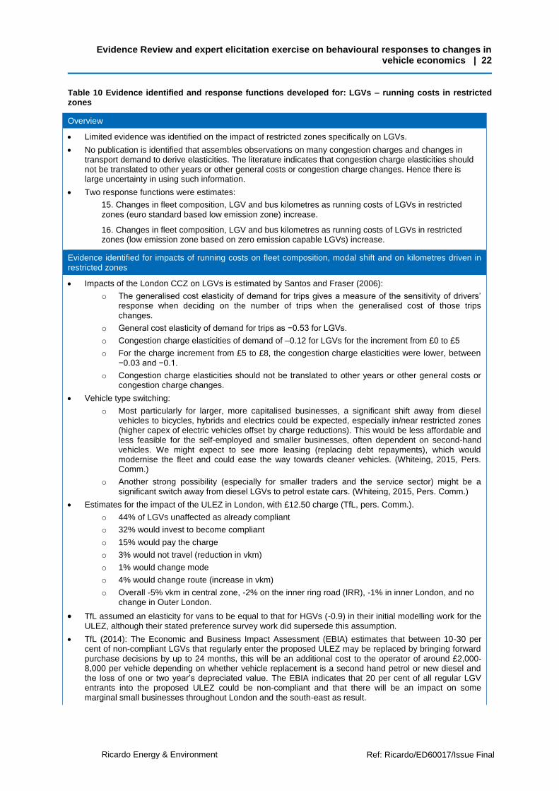
Evidence Review and expert elicitation exercise on behavioural responses to changes in vehicle economics | 22
Ricardo Energy & Environment Ref: Ricardo/ED60017/Issue Final
Table 10 Evidence identified and response functions developed for: LGVs – running costs in restricted zones
Overview
Limited evidence was identified on the impact of restricted zones specifically on LGVs.
No publication is identified that assembles observations on many congestion charges and changes in transport demand to derive elasticities. The literature indicates that congestion charge elasticities should not be translated to other years or other general costs or congestion charge changes. Hence there is large uncertainty in using such information.
Two response functions were estimates:
15. Changes in fleet composition, LGV and bus kilometres as running costs of LGVs in restricted zones (euro standard based low emission zone) increase.
16. Changes in fleet composition, LGV and bus kilometres as running costs of LGVs in restricted zones (low emission zone based on zero emission capable LGVs) increase.
Evidence identified for impacts of running costs on fleet composition, modal shift and on kilometres driven in restricted zones
Impacts of the London CCZ on LGVs is estimated by Santos and Fraser (2006):
o The generalised cost elasticity of demand for trips gives a measure of the sensitivity of drivers’ response when deciding on the number of trips when the generalised cost of those trips changes.
o General cost elasticity of demand for trips as −0.53 for LGVs.
o Congestion charge elasticities of demand of –0.12 for LGVs for the increment from £0 to £5
o For the charge increment from £5 to £8, the congestion charge elasticities were lower, between −0.03 and −0.1.
o Congestion charge elasticities should not be translated to other years or other general costs or congestion charge changes.
Vehicle type switching:
o Most particularly for larger, more capitalised businesses, a significant shift away from diesel vehicles to bicycles, hybrids and electrics could be expected, especially in/near restricted zones (higher capex of electric vehicles offset by charge reductions). This would be less affordable and less feasible for the self-employed and smaller businesses, often dependent on second-hand vehicles. We might expect to see more leasing (replacing debt repayments), which would modernise the fleet and could ease the way towards cleaner vehicles. (Whiteing, 2015, Pers. Comm.)
o Another strong possibility (especially for smaller traders and the service sector) might be a significant switch away from diesel LGVs to petrol estate cars. (Whiteing, 2015, Pers. Comm.)
Estimates for the impact of the ULEZ in London, with £12.50 charge (TfL, pers. Comm.).
o 44% of LGVs unaffected as already compliant
o 32% would invest to become compliant
o 15% would pay the charge
o 3% would not travel (reduction in vkm)
o 1% would change mode
o 4% would change route (increase in vkm)
o Overall -5% vkm in central zone, -2% on the inner ring road (IRR), -1% in inner London, and no change in Outer London.
TfL assumed an elasticity for vans to be equal to that for HGVs (-0.9) in their initial modelling work for the ULEZ, although their stated preference survey work did supersede this assumption.
TfL (2014): The Economic and Business Impact Assessment (EBIA) estimates that between 10-30 per cent of non-compliant LGVs that regularly enter the proposed ULEZ may be replaced by bringing forward purchase decisions by up to 24 months, this will be an additional cost to the operator of around £2,000-8,000 per vehicle depending on whether vehicle replacement is a second hand petrol or new diesel and the loss of one or two year’s depreciated value. The EBIA indicates that 20 per cent of all regular LGV entrants into the proposed ULEZ could be non-compliant and that there will be an impact on some marginal small businesses throughout London and the south-east as result.
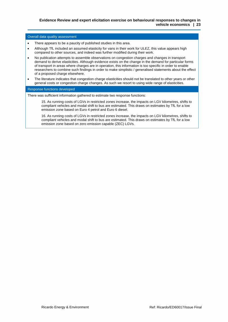
Evidence Review and expert elicitation exercise on behavioural responses to changes in vehicle economics | 23
Ricardo Energy & Environment Ref: Ricardo/ED60017/Issue Final
Overall data quality assessment
There appears to be a paucity of published studies in this area.
Although TfL included an assumed elasticity for vans in their work for ULEZ, this value appears high compared to other sources, and indeed was further modified during their work.
No publication attempts to assemble observations on congestion charges and changes in transport demand to derive elasticities. Although evidence exists on the change in the demand for particular forms of transport in areas where charges are in operation, this information is too specific in order to enable researchers to combine such findings in order to make simplistic / generalised statements about the effect of a proposed charge elsewhere.
The literature indicates that congestion charge elasticities should not be translated to other years or other general costs or congestion charge changes. As such we resort to using wide range of elasticities.
Response functions developed
There was sufficient information gathered to estimate two response functions:
15. As running costs of LGVs in restricted zones increase, the impacts on LGV kilometres, shifts to compliant vehicles and modal shift to bus are estimated. This draws on estimates by TfL for a low emission zone based on Euro 4 petrol and Euro 6 diesel.
16. As running costs of LGVs in restricted zones increase, the impacts on LGV kilometres, shifts to compliant vehicles and modal shift to bus are estimated. This draws on estimates by TfL for a low emission zone based on zero emission capable (ZEC) LGVs.

Evidence Review and expert elicitation exercise on behavioural responses to changes in vehicle economics | 24
Ricardo Energy & Environment Ref: Ricardo/ED60017/Issue Final
4.3.3 Evidence identified for HGVs
Table 11 Evidence identified and response functions developed for: HGVs – upfront costs
Overview
No quantitative evidence identified.
Although evidence was identified on the relative costs of gas from diesel trucks, the possible behavioural response to changes in gas truck prices was not possible to identify from literature or from the expert panel.
One response function was estimated, which has high uncertainty :
18. Change in HGV kilometres driven as upfront costs of HGVs change.
Evidence identified for impacts of purchase costs on fleet composition, modal shift and on kilometres driven
It is expected that given a choice, more operators purchase new EURO VI compliant vehicles rather than retrofitting of modifications to older vehicles (Whiteing, Pers. Comm.). Only relatively new vehicles would be worth modifying. As with the LGV fleet, it is expected that the larger more capitalised fleets invest in the latest vehicles, especially when working for major blue-chip clients such as major manufacturers or retailers where image and green credentials may be more telling. (Whiteing, Pers. comm.)
Increases in the upfront purchase cost of HGVs of 2% to 20% represent a relatively small proportion of total fleet operating costs, and for larger fleet operators these costs are probably affordable. For small operators and owner-operators typically operating on very tight margins, affordability is much more of an issue. If these companies cannot afford modern greener vehicles and hence face operating cost penalties and/or exclusion from restricted zones, this could lead to increasing concentration of fleets into the larger companies. (Whiteing, Pers. comm.).
The higher end of the range 2-20% for changing the upfront HGV cost could encourage a shift to Euro VI (gas and diesel) (Personal Communication, LowCVP).
Upfront cost increases of conventional diesel HGVs would encourage greater shifting to gas powered HGVs, whether as dual fuel or pure gas CNG/LNG. Numerous barriers to implementation have been recognised in the literature (Ricardo-AEA, 2012; DfT 2014c), including provision of gas refuelling infrastructure, uncertainty over future tax regimes, relative diesel / gas prices.
For gas trucks, the upfront costs of gas HGVs have been indicated to be between £15,000 and £44,000 more than diesel equivalents, with maintenance costs between 10% and 40% higher. Fuel savings may be of the order of £7,000 to £15,000 per annum for high mileages (higher than those assumed in Table 3 for articulated HGVs. These figures suggest payback periods of between 2 and 8 years, which would indicate that operators ought to already be considering.
No literature could be identified nor were experts willing to suggest possible take-up rates for purchase of gas trucks at given upfront cost reductions.
There is also uncertainty over the possible NOX savings of gas trucks over diesel trucks. These uncertainties include: mixed evidence from very limited trials, uncertain diesel / gas mix in the dual fuel engines, and limited availability of Euro VI compliant gas trucks. LowCVP indicated that a number of dual fuel technologies cannot at present meet Euro VI – and that this is being explored as part of the Low Carbon Trust Trial – and hence that additional technologies would be needed to meet Euro VI. Therefore the additional benefits over diesel Euro VI which also use end of pipe NOX abatement are unclear.
Overall data quality assessment
No quantitative information identified to support a relationship between changes in purchase costs and impacts on fleet composition or vehicle kilometres.
Although no response function could be estimated for gas trucks, any upfront cost reduction measures would make the purchase of gas trucks more favourable from the present very low levels of uptake. Infrastructure support measures would also assist.
Response functions developed
One response function has been estimated:
18. Change in HGV kilometres driven as upfront costs of HGVs change. As no evidence was identified relating HGV distances travelled with purchase costs, elasticities for HGV running costs were used with upfront cost changes converted into running cost changes (total cost of ownership approach). Estimated impacts on rail freight are also estimated.

Evidence Review and expert elicitation exercise on behavioural responses to changes in vehicle economics | 25
Ricardo Energy & Environment Ref: Ricardo/ED60017/Issue Final
Table 12 Evidence identified and response functions developed for: HGVs – running costs
Overview
Road freight cost elasticities identified in the literature, and expert panel suggestion for adjustment of these.
Elasticities derived from one literature source for modal shift to rail
One response function was estimated:
9. Changes in HGV kilometres driven as HGV running costs change.
Evidence identified for impacts of running costs on fleet composition and vehicle kilometres
Given daily articulated HGV running costs exceed £500 (of which fuel costs roughly one third), price perturbations in the range of £20 to £200/day are within the range of elasticity validity.
Elasticities found in the literature:
o Road freight cost elasticities (not clear if on km or t-km basis) estimated to vary widely but are generally believed to be the range -0.6 to -1.3. Value of -0.84 is shown by Graham and Glaister (2004) to be a modal value.
o Whiteing (pers. Comm.) view that -0.84 should be upper end of range, and that range -0.5 to -0.8 would be more likely for running cost elasticities, taking into account pass through of costs and that running costs are only a part of total costs.
o Fuel price elasticities with respect to vkm: -0.1 to -0.6 (RAND Europe, 2014) and -0.2 (de Jong et al., 2010)
o Vehicle km price elasticity with respect to vkm: -0.9 (de Jong et al., 2010)
o –0.21 to –0.30 (Ramli and Graham, 2014)
The elasticity values are higher than for cars, which is consistent with the understanding that there is greater flexibility in logistic patterns.
Imposition of increased costs likely to change / reorganise systems, e.g. distribution centres relocated close to markets, with more, smaller distribution hubs. Threshold effects / tipping points are undoubtedly likely to occur but they are very difficult to estimate in the aggregate case, because they are likely to happen at different levels of cost increase for different traffics and commodities and in different business circumstances. They would happen earlier for those commodities and traffics most amenable to model shift, and later for those traffics for which the advantages of road freight are greatest and where transport costs may be a small percentage of product value. Relatively high increases in running costs would encourage more local sourcing. Bulky low-value products would be a case in point – Scottish potatoes and turnips are frequently sold in English supermarkets, but they would not compete with more local sources if transport costs rose significantly.
Switch to rail freight is possible for longer distance flows and where distribution depots exist or could be built at which freight is transferred to road for the final stage of the trip. The impact on exceedances will be very dependent on the specific journey. Operators re-assess their logistics fairly frequently. A 75% increase in fuel pump price (following fourfold increase in oil commodity cost) has been modelled as reducing HGV vehicle km by 11%, increasing rail freight by 13% and reducing overall freight demand (Fowkes et al, 2010). The implied fuel cost elasticity here is -0.11/0.75 = -0.15. With daily fuel costs assumed to be around £160, a 75% increase would be £120.
Overall data quality assessment
No information available on impacts on the fleet composition.
Limited literature available on modal shift.
Some literature identified including meta-analyses on fuel cost elasticities.
Response functions developed
One response function has been estimated:
9. As running costs of all HGVs change, HGV kilometres driven are estimated using cost elasticities. The range of elasticities from literature are used for lower (Fowkes et al., 2010) and upper bounds (Graham and Glaister, 2004); the central estimate is based on suggestion by the expert panel.
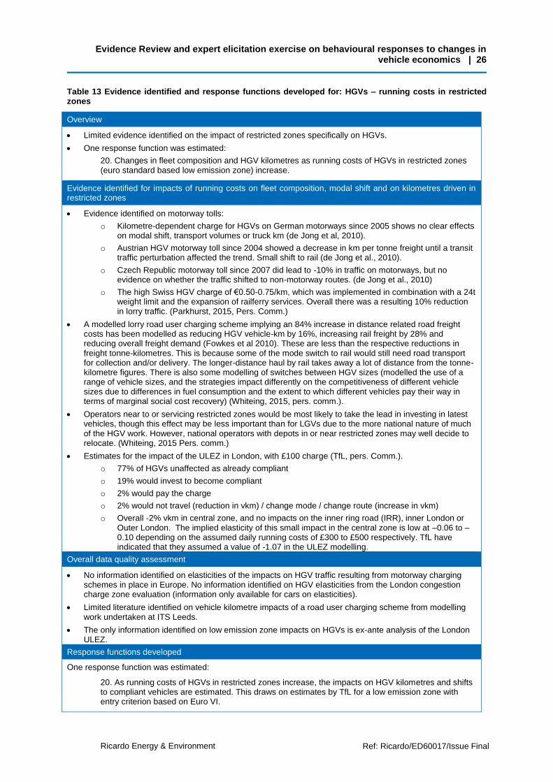
Evidence Review and expert elicitation exercise on behavioural responses to changes in vehicle economics | 26
Ricardo Energy & Environment Ref: Ricardo/ED60017/Issue Final
Table 13 Evidence identified and response functions developed for: HGVs – running costs in restricted zones
Overview
Limited evidence identified on the impact of restricted zones specifically on HGVs.
One response function was estimated:
20. Changes in fleet composition and HGV kilometres as running costs of HGVs in restricted zones (euro standard based low emission zone) increase.
Evidence identified for impacts of running costs on fleet composition, modal shift and on kilometres driven in restricted zones
Evidence identified on motorway tolls:
o Kilometre-dependent charge for HGVs on German motorways since 2005 shows no clear effects on modal shift, transport volumes or truck km (de Jong et al, 2010).
o Austrian HGV motorway toll since 2004 showed a decrease in km per tonne freight until a transit traffic perturbation affected the trend. Small shift to rail (de Jong et al., 2010).
o Czech Republic motorway toll since 2007 did lead to -10% in traffic on motorways, but no evidence on whether the traffic shifted to non-motorway routes. (de Jong et al., 2010)
o The high Swiss HGV charge of €0.50-0.75/km, which was implemented in combination with a 24t weight limit and the expansion of railferry services. Overall there was a resulting 10% reduction in lorry traffic. (Parkhurst, 2015, Pers. Comm.)
A modelled lorry road user charging scheme implying an 84% increase in distance related road freight costs has been modelled as reducing HGV vehicle-km by 16%, increasing rail freight by 28% and reducing overall freight demand (Fowkes et al 2010). These are less than the respective reductions in freight tonne-kilometres. This is because some of the mode switch to rail would still need road transport for collection and/or delivery. The longer-distance haul by rail takes away a lot of distance from the tonne-kilometre figures. There is also some modelling of switches between HGV sizes (modelled the use of a range of vehicle sizes, and the strategies impact differently on the competitiveness of different vehicle sizes due to differences in fuel consumption and the extent to which different vehicles pay their way in terms of marginal social cost recovery) (Whiteing, 2015, pers. comm.).
Operators near to or servicing restricted zones would be most likely to take the lead in investing in latest vehicles, though this effect may be less important than for LGVs due to the more national nature of much of the HGV work. However, national operators with depots in or near restricted zones may well decide to relocate. (Whiteing, 2015 Pers. comm.)
Estimates for the impact of the ULEZ in London, with £100 charge (TfL, pers. Comm.).
o 77% of HGVs unaffected as already compliant
o 19% would invest to become compliant
o 2% would pay the charge
o 2% would not travel (reduction in vkm) / change mode / change route (increase in vkm)
o Overall -2% vkm in central zone, and no impacts on the inner ring road (IRR), inner London or Outer London. The implied elasticity of this small impact in the central zone is low at –0.06 to –0.10 depending on the assumed daily running costs of £300 to £500 respectively. TfL have indicated that they assumed a value of -1.07 in the ULEZ modelling.
Overall data quality assessment
No information identified on elasticities of the impacts on HGV traffic resulting from motorway charging schemes in place in Europe. No information identified on HGV elasticities from the London congestion charge zone evaluation (information only available for cars on elasticities).
Limited literature identified on vehicle kilometre impacts of a road user charging scheme from modelling work undertaken at ITS Leeds.
The only information identified on low emission zone impacts on HGVs is ex-ante analysis of the London ULEZ.
Response functions developed
One response function was estimated:
20. As running costs of HGVs in restricted zones increase, the impacts on HGV kilometres and shifts to compliant vehicles are estimated. This draws on estimates by TfL for a low emission zone with entry criterion based on Euro VI.

Evidence Review and expert elicitation exercise on behavioural responses to changes in vehicle economics | 27
Ricardo Energy & Environment Ref: Ricardo/ED60017/Issue Final
4.3.4 Evidence identified for buses
Table 14 Evidence identified and response functions developed for: Buses – upfront costs
Overview
No quantitative evidence identified.
One response function was estimated, which has high uncertainty :
8. Change in bus kilometres, car kilometres and passenger rail demand as upfront costs of buses change.
Evidence identified for impacts of purchase costs on fleet composition, modal shift and on kilometres driven
No evidence was identified that quantifies the relationship between bus purchase costs and kilometres driven or mode shift.
Purchase cost would be expected to affect choice of technology. E.g. OLEV grants in relation to capital cost are considered to have stimulated the uptake of most of the hybrid, electric and gas buses in the UK.
Bus operators typically take a total cost of ownership approach.
Purchase costs are estimated to make up 15% of total costs of ownership.
Overall data quality assessment
No quantitative evidence identified
Response functions developed
One response function has been estimated:
8. Change in bus kilometres, car kilometres and passenger rail demand as upfront costs of buses change. As no evidence was identified relating these variables directly with purchase costs, elasticities for bus running costs were used with upfront cost changes converted into running cost changes (total cost of ownership approach). Estimated impacts on passenger rail demand are also estimated.
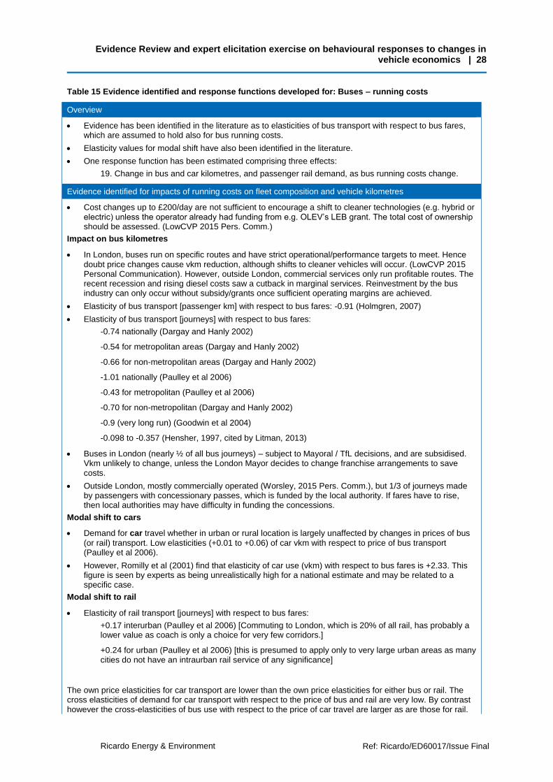
Evidence Review and expert elicitation exercise on behavioural responses to changes in vehicle economics | 28
Ricardo Energy & Environment Ref: Ricardo/ED60017/Issue Final
Table 15 Evidence identified and response functions developed for: Buses – running costs
Overview
Evidence has been identified in the literature as to elasticities of bus transport with respect to bus fares, which are assumed to hold also for bus running costs.
Elasticity values for modal shift have also been identified in the literature.
One response function has been estimated comprising three effects:
19. Change in bus and car kilometres, and passenger rail demand, as bus running costs change.
Evidence identified for impacts of running costs on fleet composition and vehicle kilometres
Cost changes up to £200/day are not sufficient to encourage a shift to cleaner technologies (e.g. hybrid or electric) unless the operator already had funding from e.g. OLEV’s LEB grant. The total cost of ownership should be assessed. (LowCVP 2015 Pers. Comm.)
Impact on bus kilometres
In London, buses run on specific routes and have strict operational/performance targets to meet. Hence doubt price changes cause vkm reduction, although shifts to cleaner vehicles will occur. (LowCVP 2015 Personal Communication). However, outside London, commercial services only run profitable routes. The recent recession and rising diesel costs saw a cutback in marginal services. Reinvestment by the bus industry can only occur without subsidy/grants once sufficient operating margins are achieved.
Elasticity of bus transport [passenger km] with respect to bus fares: -0.91 (Holmgren, 2007)
Elasticity of bus transport [journeys] with respect to bus fares:
-0.74 nationally (Dargay and Hanly 2002)
-0.54 for metropolitan areas (Dargay and Hanly 2002)
-0.66 for non-metropolitan areas (Dargay and Hanly 2002)
-1.01 nationally (Paulley et al 2006)
-0.43 for metropolitan (Paulley et al 2006)
-0.70 for non-metropolitan (Dargay and Hanly 2002)
-0.9 (very long run) (Goodwin et al 2004)
-0.098 to -0.357 (Hensher, 1997, cited by Litman, 2013)
Buses in London (nearly ½ of all bus journeys) – subject to Mayoral / TfL decisions, and are subsidised. Vkm unlikely to change, unless the London Mayor decides to change franchise arrangements to save costs.
Outside London, mostly commercially operated (Worsley, 2015 Pers. Comm.), but 1/3 of journeys made by passengers with concessionary passes, which is funded by the local authority. If fares have to rise, then local authorities may have difficulty in funding the concessions.
Modal shift to cars
Demand for car travel whether in urban or rural location is largely unaffected by changes in prices of bus
(or rail) transport. Low elasticities (+0.01 to +0.06) of car vkm with respect to price of bus transport (Paulley et al 2006).
However, Romilly et al (2001) find that elasticity of car use (vkm) with respect to bus fares is +2.33. This figure is seen by experts as being unrealistically high for a national estimate and may be related to a specific case.
Modal shift to rail
Elasticity of rail transport [journeys] with respect to bus fares:
+0.17 interurban (Paulley et al 2006) [Commuting to London, which is 20% of all rail, has probably a lower value as coach is only a choice for very few corridors.]
+0.24 for urban (Paulley et al 2006) [this is presumed to apply only to very large urban areas as many cities do not have an intraurban rail service of any significance]
The own price elasticities for car transport are lower than the own price elasticities for either bus or rail. The cross elasticities of demand for car transport with respect to the price of bus and rail are very low. By contrast however the cross-elasticities of bus use with respect to the price of car travel are larger as are those for rail.

Evidence Review and expert elicitation exercise on behavioural responses to changes in vehicle economics | 29
Ricardo Energy & Environment Ref: Ricardo/ED60017/Issue Final
What this points to is that reducing the price of public transport will not reduce the demand for private transport but might instead generate trips from those who might not otherwise have travelled.
Overall data quality assessment
There is quite some variation in literature estimates of bus elasticities. This probably reflects the wide variation across the country in terms of demand, rail provision, relative wealth
The above elasticities related to bus fares are assumed to hold also for bus running costs on the basis that small margins in this sector lead to pass through of running cost increases as fare rises.
Rail impacts are likely very location specific given the limited catchment of rail unless car access to rail is factored in.
Response functions developed
One response function has been estimated comprising three effects:
19. As running costs of all buses change, bus kilometres, car kilometres and passenger rail demand are estimated using elasticities. Different elasticities are used for low central and upper bounds.

Evidence Review and expert elicitation exercise on behavioural responses to changes in vehicle economics | 30
Ricardo Energy & Environment Ref: Ricardo/ED60017/Issue Final
Table 16 Evidence identified and response functions developed for: Buses – running costs in restricted zones
Overview
Limited evidence identified on the impact of restricted zones specifically on buses and coaches.
One response function was estimated, applicable to buses and coaches:
17. Changes in fleet composition and bus kilometres as running costs of buses in restricted zones (Euro VI based low emission zone) increase.
Evidence identified for impacts of running costs on fleet composition, modal shift and on kilometres driven in restricted zones
Estimates for the impact of the ULEZ in London, with £100 charge (TfL, pers. Comm.).
o 67% of coaches would be unaffected as already compliant
o 23% would invest to become compliant. Unlike the case of buses, the coach industry is profitable and very low subsidy. Reinvestment is more possible and likely.
o 5% would pay the charge
o 4% would not travel (reduction in vkm) / change mode / change route (increase in vkm)
o Overall TfL expects for coaches -4% vkm in central zone, -1% on IRR and in inner London, and no change in Outer London.
Other than in London, coach operators are seeking to reduce exposure to congestion in urban areas by stopping at peripheral locations. Restrictions might encourage this trend so the vehicles do not need to enter the restriction zone (Parkhurst, 2015, Pers. Comm.).
No impact on passenger fares expected in London buses.
TfL (2014): The ULEZ EBIA estimates that between 10- 30 per cent of non-compliant vehicles that regularly enter London may be replaced by bringing forward purchase decisions by up to 24 months, this will be an additional cost to the operator of around £5-10,000 per vehicle and the loss of one or two year’s depreciated value). Where vehicles are not able to be replaced as part of an existing vehicle replacement cycle, the additional costs incurred (either through vehicle purchases or payment of the ULEZ charge for non-compliance) could be passed onto the users of the services.
Overall data quality assessment
No information identified for impacts outside of London. No specific elasticity information to cover the country sufficiently. Small negative elasticity expected.
Within London, the policy is designed around the existing bus fleet.
The impacts on coaches in London of ULEZ have been estimated, but not with elasticities. No modal shift information identified.
Response functions developed
One response function was estimated:
17. As running costs of buses in restricted zones increase, the impacts on bus kilometres and shifts to compliant vehicles (fleet composition changes) are estimated. This draws on estimates by TfL for a low emission zone with entry criterion based on Euro VI.
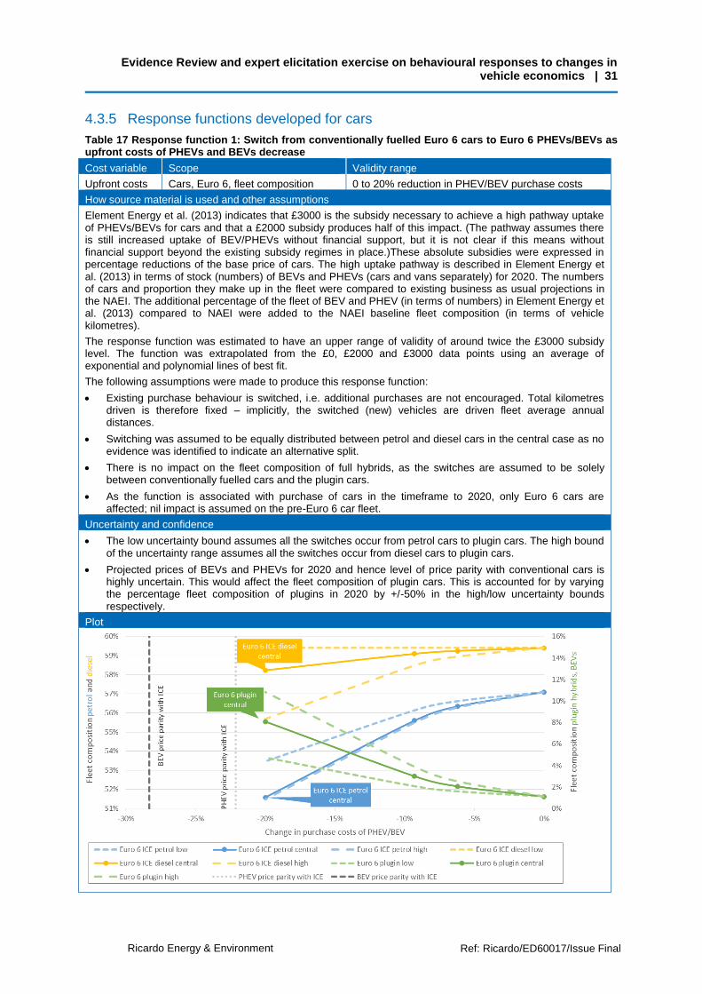
Evidence Review and expert elicitation exercise on behavioural responses to changes in vehicle economics | 31
Ricardo Energy & Environment Ref: Ricardo/ED60017/Issue Final
4.3.5 Response functions developed for cars
Table 17 Response function 1: Switch from conventionally fuelled Euro 6 cars to Euro 6 PHEVs/BEVs as upfront costs of PHEVs and BEVs decrease
Cost variable Scope Validity range
Upfront costs Cars, Euro 6, fleet composition 0 to 20% reduction in PHEV/BEV purchase costs
How source material is used and other assumptions
Element Energy et al. (2013) indicates that £3000 is the subsidy necessary to achieve a high pathway uptake of PHEVs/BEVs for cars and that a £2000 subsidy produces half of this impact. (The pathway assumes there is still increased uptake of BEV/PHEVs without financial support, but it is not clear if this means without financial support beyond the existing subsidy regimes in place.)These absolute subsidies were expressed in percentage reductions of the base price of cars. The high uptake pathway is described in Element Energy et al. (2013) in terms of stock (numbers) of BEVs and PHEVs (cars and vans separately) for 2020. The numbers of cars and proportion they make up in the fleet were compared to existing business as usual projections in the NAEI. The additional percentage of the fleet of BEV and PHEV (in terms of numbers) in Element Energy et al. (2013) compared to NAEI were added to the NAEI baseline fleet composition (in terms of vehicle kilometres).
The response function was estimated to have an upper range of validity of around twice the £3000 subsidy level. The function was extrapolated from the £0, £2000 and £3000 data points using an average of exponential and polynomial lines of best fit.
The following assumptions were made to produce this response function:
Existing purchase behaviour is switched, i.e. additional purchases are not encouraged. Total kilometres driven is therefore fixed – implicitly, the switched (new) vehicles are driven fleet average annual distances.
Switching was assumed to be equally distributed between petrol and diesel cars in the central case as no evidence was identified to indicate an alternative split.
There is no impact on the fleet composition of full hybrids, as the switches are assumed to be solely between conventionally fuelled cars and the plugin cars.
As the function is associated with purchase of cars in the timeframe to 2020, only Euro 6 cars are affected; nil impact is assumed on the pre-Euro 6 car fleet.
Uncertainty and confidence
The low uncertainty bound assumes all the switches occur from petrol cars to plugin cars. The high bound of the uncertainty range assumes all the switches occur from diesel cars to plugin cars.
Projected prices of BEVs and PHEVs for 2020 and hence level of price parity with conventional cars is highly uncertain. This would affect the fleet composition of plugin cars. This is accounted for by varying the percentage fleet composition of plugins in 2020 by +/-50% in the high/low uncertainty bounds respectively.
Plot

Evidence Review and expert elicitation exercise on behavioural responses to changes in vehicle economics | 32
Ricardo Energy & Environment Ref: Ricardo/ED60017/Issue Final
Table 18 Response function 3: Reduction in purchase of conventionally fuelled Euro 6 cars as upfront costs of conventionally fuelled cars increase, and limited switch to alternatively fuelled vehicles (hybrids, PHEVs, BEVs)
Cost variable Scope Validity range
Upfront costs Euro 6 car vehicle kilometres 0 to 20% increase in ICE purchase costs
How source material is used and other assumptions
This response function draws on literature estimates of elasticity of car ownership with respect to purchase costs. The central estimate is chosen to be -0.34 (Whelan, 2007) as this is a recent source and is used in DfT modelling. The low bound of uncertainty is -0.1 (Goodwin et al., 2004), and the high bound -0.5 (implied in Eftec, 2008). For increasing purchase costs of conventionally fuelled petrol and diesel vehicles, these elasticity estimates are used to estimate the reductions in number of Euro 6 conventionally fuelled petrol and diesel cars bought for each year from an assumed policy start year and cumulative to 2020. The change to the vehicle kilometres of the Euro 6 petrol and diesel cars is then estimated directly for 2020 by assuming these vehicles are driven average distances for all cars. New vehicle registrations for each car type and for each year are estimated by projecting 2014 SMMT new car registration data (SMMT, 2014) with the annual average growth rates implied by NAEI car fleet stock 2015 and 2020 projections. This projection implicitly assumes that new registrations of petrol cars do not decline over this period and that the overall petrol car stock reduction is due to overall a larger number of (older) petrol cars retired from the fleet than (new) added to the fleet. The estimates of this projection for 2020 are the following numbers of new cars: 1.2bn petrol cars, 1.3bn diesel cars, 130,000 hybrid petrol cars, 75,000 hybrid diesel cars, 150,000 plugin hybrid cars and 80,000 full electric cars.
It is assumed that the hypothetical policy measure applies a price increment to some vehicles (conventionally fuelled cars) but not all vehicles, and hence that a small proportion of car buyers that decide not to buy a conventionally fuelled car choose instead purchase an alternatively fuelled vehicle (which may be more expensive). Changes in numbers of alternative fuelled vehicles and their vehicles kilometres driven are estimated using the inverse of the above described elasticities for the low, central and high scenarios.
The following assumptions were made to produce this response function:
The policy start date is a user input variable from 2016 to 2020.
The petrol / diesel car split would change because of the four alternative fuelled vehicle types, only one is diesel.
No rebound effect estimated.
Only Euro 6 cars are assumed to be affected; nil impacts are assumed for pre-Euro 6 cars.
Uncertainty and confidence
High uncertainty of the projected registrations of new alternative fuelled vehicles. Highly uncertain total uptake rates of alternative fuelled vehicles (assumed to be non-zero) if the purchase price of conventionally fuelled vehicles is increased. High uncertainty of the relative split among the different alternative fuelled cars (hybrid petrol, hybrid diesel, PHEV and BEV).
Plot [for central estimate, assuming policy start year of 2018]
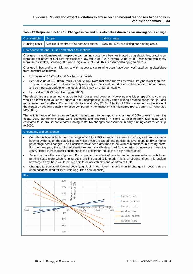
Evidence Review and expert elicitation exercise on behavioural responses to changes in vehicle economics | 33
Ricardo Energy & Environment Ref: Ricardo/ED60017/Issue Final
Table 19 Response function 12: Changes in car and bus kilometres driven as car running costs change
Cost variable Scope Validity range
Running costs Vehicle kilometres of all cars and buses -50% to +50% of existing car running costs
How source material is used and other assumptions
Changes in car kilometres with respect to car running costs have been estimated using elasticities, drawing on literature estimates of fuel cost elasticities: a low value of -0.2, a central value of -0.3 consistent with many literature estimates, including DfT; and a high value of -0.4. This is assumed to apply to all cars.
Changes in bus and coach kilometres with respect to car running costs have been estimated using elasticities from literature as follows:
Low value of 0.1 (Turcksin & Macharis, undated)
Central value of 0.55 (from Paulley et al., 2006). Note that short run values would likely be lower than this. This value is selected as it was the only elasticity in the literature indicated to be specific to urban buses, and so most appropriate for the focus of this study on urban air quality.
High value of 0.73 (from Holmgren, 2007)
The elasticities are assumed to apply to both buses and coaches. However, elasticities specific to coaches would be lower than values for buses due to uncompetitive journey times of long distance coach market, and more limited market (Pers. Comm. with G. Parkhurst, May 2015). A factor of 15% is assumed for the scale of the impact on bus and coach kilometres compared to the impact on car kilometres (Pers. Comm. G. Parkhurst, May 2015).
The validity range of the response function is assumed to be capped at changes of 50% of existing running costs. Daily car running costs were estimated and described in Table 2. Most notably, fuel costs were estimated to be around half of total running costs. No changes are assumed in daily running costs for cars up to 2020.
Uncertainty and confidence
Confidence level is high over the range of a 0 to +10% change in car running costs, as there is a large body of evidence on the elasticities on which these are based. The confidence level drops to low at higher percentage cost changes. The elasticities have been assumed to be valid at reductions in running costs. For the most part, the published elasticities are typically described for scenarios of increases in running costs. Hence there is lower confidence in the effects for reductions in car running costs.
Second order effects are ignored. For example, the effect of people tending to use vehicles with lower running costs more when running costs are increased is ignored. This is a rebound effect. It is unclear how large if any there would be in a shift to newer vehicles and/or different fuels
Changes to perceived running costs (e.g. fuel) have higher impacts than to changes in costs that are often not accounted for by drivers (e.g. fixed annual costs).
Plot

Evidence Review and expert elicitation exercise on behavioural responses to changes in vehicle economics | 34
Ricardo Energy & Environment Ref: Ricardo/ED60017/Issue Final
Table 20 Response function 6: Changes in fleet composition due to switches from conventionally to alternatively fuelled Euro 6 cars as running costs of conventionally fuelled cars increases.
Cost variable Scope Validity range
Running costs Euro 6 car fleet composition, vkm 0 to +39% of existing car running costs
How source material is used and other assumptions
The function assumes a policy driver increases the running costs of conventionally fuelled cars leading to Euro 6 hybrids and plugins to be bought instead of Euro 6 conventionally fuelled cars. The function is based on Turcksin & Macharis (undated) who undertook a survey of drivers in Belgium. Respondents were asked to indicate the running cost increase threshold at which they would consider purchasing a cleaner version of their preferred car. For running costs, they were asked to consider responses separately for an annual pollution charge and a km-based charge; an average of these responses is assumed for this function. It is assumed that “cleaner” is a mixture of petrol hybrids, diesel hybrids, plugin hybrid (petrol) and BEVs, and the mix between these is assumed to be the same mix assumed in the 2020 projections in the NAEI. Cumulative fleet impacts are estimated for year 2020 from changes in the numbers of vehicles purchased each year by type. The petrol / diesel car split changes because of how the alternative fuelled vehicle types are categorised.
The absolute increases in Belgian running costs from the study are converted to percentage daily increases through estimating daily running costs of vehicles in Belgium. Daily car running costs in Belgium were estimated to be 20% higher than in the UK due to: (1) higher annual distance travelled at 15,000km compared to assumed 12,700km for UK and so higher fuel costs (Turcksin and Macharis, undated) and (2) higher average tax (including an annual €127 premium levied on diesel vehicles). The differences in average upfront costs between BE and UK were not taken into account.
The upper bound of validity is taken from the survey results – i.e. the increase in running costs at which 100% of respondents would switch.
The following additional assumptions were made to produce this response function:
The policy start date is a user input variable from 2016 to 2020.
The total stock of vehicles is assumed constant – i.e. existing purchase decisions are simply switched.
Only Euro 6 cars are assumed to be affected; nil impacts are assumed for pre-Euro 6 cars.
The alternative fuelled vehicles are assumed to driver lower than average car distances, meaning that overall vehicle kilometres reduce with increasing running costs.
No rebound effect estimated.
Uncertainty and confidence
This function is based on a single survey of around 1,700 Belgian drivers, and so confidence levels in the behavioural response are low. In particular, it is uncertain how survey responders would actually behaviour for a purchase decision compared to how they indicated they would behave in a survey. Consequently, a wide uncertainty range is stipulated. The low bound of uncertainty assumes a 50% lower response rate of drivers than as declared in the survey. The high bound of uncertainty assumes a 50% higher response rate of drivers until 100% of drivers is reached.
There is high uncertainty of the relative split among the different alternative fuelled cars (hybrid petrol, hybrid diesel, PHEV and BEV).
Plot (central case, assuming policy start year of 2018)
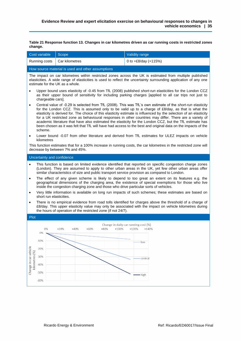
Evidence Review and expert elicitation exercise on behavioural responses to changes in vehicle economics | 35
Ricardo Energy & Environment Ref: Ricardo/ED60017/Issue Final
Table 21 Response function 13. Changes in car kilometres driven as car running costs in restricted zones change.
Cost variable Scope Validity range
Running costs Car kilometres 0 to +£8/day (+115%)
How source material is used and other assumptions
The impact on car kilometres within restricted zones across the UK is estimated from multiple published elasticities. A wide range of elasticities is used to reflect the uncertainty surrounding application of any one estimate for the UK as a whole.
Upper bound uses elasticity of -0.45 from TfL (2008) published short-run elasticities for the London CCZ as their upper bound of sensitivity for including parking charges [applied to all car trips not just to chargeable cars].
Central value of -0.29 is selected from TfL (2008). This was TfL’s own estimate of the short-run elasticity for the London CCZ. This is assumed only to be valid up to a charge of £8/day, as that is what the elasticity is derived for. The choice of this elasticity estimate is influenced by the selection of an elasticity for a UK restricted zone as behavioural responses in other countries may differ. There are a variety of academic literature that have also estimated the elasticity for the London CCZ, but the TfL estimate has been chosen as it was felt that TfL will have had access to the best and original data on the impacts of the scheme.
Lower bound -0.07 from other literature and derived from TfL estimates for ULEZ impacts on vehicle kilometres
This function estimates that for a 100% increase in running costs, the car kilometres in the restricted zone will decrease by between 7% and 45%.
Uncertainty and confidence
This function is based on limited evidence identified that reported on specific congestion charge zones (London). They are assumed to apply to other urban areas in the UK, yet few other urban areas offer similar characteristics of size and public transport service provision as compared to London.
The effect of any given scheme is likely to depend to too great an extent on its features e.g. the geographical dimensions of the charging area, the existence of special exemptions for those who live inside the congestion charging zone and those who drive particular sorts of vehicles.
Very little information is available on long run impacts of such schemes; these estimates are based on short run elasticities.
There is no empirical evidence from road tolls identified for charges above the threshold of a charge of £8/day. This upper elasticity value may only be associated with the impact on vehicle kilometres during the hours of operation of the restricted zone (if not 24/7).
Plot
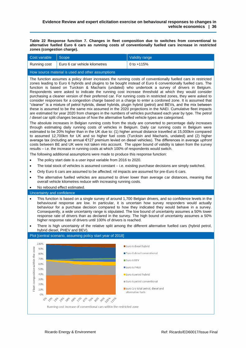
Evidence Review and expert elicitation exercise on behavioural responses to changes in vehicle economics | 36
Ricardo Energy & Environment Ref: Ricardo/ED60017/Issue Final
Table 22 Response function 7. Changes in fleet composition due to switches from conventional to alternative fuelled Euro 6 cars as running costs of conventionally fuelled cars increase in restricted zones (congestion charge).
Cost variable Scope Validity range
Running cost Euro 6 car vehicle kilometres 0 to +115%
How source material is used and other assumptions
The function assumes a policy driver increases the running costs of conventionally fuelled cars in restricted zones leading to Euro 6 hybrids and plugins to be bought instead of Euro 6 conventionally fuelled cars. The function is based on Turcksin & Macharis (undated) who undertook a survey of drivers in Belgium. Respondents were asked to indicate the running cost increase threshold at which they would consider purchasing a cleaner version of their preferred car. For running costs in restricted zones, they were asked to consider responses for a congestion charge based on a charge to enter a cordoned zone. It is assumed that “cleaner” is a mixture of petrol hybrids, diesel hybrids, plugin hybrid (petrol) and BEVs, and the mix between these is assumed to be the same mix assumed in the 2020 projections in the NAEI. Cumulative fleet impacts are estimated for year 2020 from changes in the numbers of vehicles purchased each year by type. The petrol / diesel car split changes because of how the alternative fuelled vehicle types are categorised.
The absolute increases in Belgian running costs from the study are converted to percentage daily increases through estimating daily running costs of vehicles in Belgium. Daily car running costs in Belgium were estimated to be 20% higher than in the UK due to: (1) higher annual distance travelled at 15,000km compared to assumed 12,700km for UK and so higher fuel costs (Turcksin and Macharis, undated) and (2) higher average tax (including an annual €127 premium levied on diesel vehicles). The differences in average upfront costs between BE and UK were not taken into account. The upper bound of validity is taken from the survey results – i.e. the increase in running costs at which 100% of respondents would switch.
The following additional assumptions were made to produce this response function:
The policy start date is a user input variable from 2016 to 2020.
The total stock of vehicles is assumed constant – i.e. existing purchase decisions are simply switched.
Only Euro 6 cars are assumed to be affected; nil impacts are assumed for pre-Euro 6 cars.
The alternative fuelled vehicles are assumed to driver lower than average car distances, meaning that overall vehicle kilometres reduce with increasing running costs.
No rebound effect estimated.
Uncertainty and confidence
This function is based on a single survey of around 1,700 Belgian drivers, and so confidence levels in the behavioural response are low. In particular, it is uncertain how survey responders would actually behaviour for a purchase decision compared to how they indicated they would behave in a survey. Consequently, a wide uncertainty range is stipulated. The low bound of uncertainty assumes a 50% lower response rate of drivers than as declared in the survey. The high bound of uncertainty assumes a 50% higher response rate of drivers until 100% of drivers is reached.
There is high uncertainty of the relative split among the different alternative fuelled cars (hybrid petrol, hybrid diesel, PHEV and BEV).
Plot [central scenario, assuming policy start year of 2018]

Evidence Review and expert elicitation exercise on behavioural responses to changes in vehicle economics | 37
Ricardo Energy & Environment Ref: Ricardo/ED60017/Issue Final
Table 23 Response function 4. Changes in fleet composition, car and bus kilometres as running costs of cars in restricted zones (euro standard based low emission zone) increase.
Cost variable Scope Validity range
Running cost Car, bus kilometres, fleet composition 0 to +£100/day charge (+542%)
How source material is used and other assumptions
This function estimates the impact on fleet composition and vehicle kilometres of low emission zones that have a Euro 4 petrol / Euro 6 diesel entry criterion. The central estimates are based on TfL ex ante analysis of the Ultra-Low Emission Zone (ULEZ) in London in 2020 (TfL, Pers. Comm.). TfL estimated behavioural responses for daily zone charges of £12.50 and of £100: between stay and pay, change travel behaviour, become compliant, and already compliant. These estimates have been linearly interpolated between and form the central estimate. The low and high scenarios were estimated by Ricardo Energy & Environment as the lower and upper ranges of possible behavioural responses, and checked with TfL. These show assumed 100% compliance for a charge of £100/day for all scenarios. The low [emissions] scenario is based on low vehicle kilometres driven and high compliance. The high [emissions] scenario is based on high vehicle kilometres driven and low compliance.
Charge Car vkm Split of petrol Compliant Bus vkm
Central £12.50 -5% 59% 93% +0.3%
£100 -11% 63% 100% +0.6%
Low £12.50 -23% 55% 100% 0
£100 -23% 55% 100% 0
High £12.50 -1% 59% 90% +0.7%
£100 -3% 63% 100% +2.1%
Further assumptions include:
24/7 operation of the LEZ
Existing payment of London CCZ charge (£11.50) assumed to be part of the daily running costs of cars.
Modal shift impacts have also been taken from TfL modelling: shift to bus comprises 3/8 of the drivers that change travel behaviour (TfL, Pers. Comm.), and that bus kilometres impacts are 15% that of cars.
The base case (£0 charge) assumes fleet composition of the NAEI (77% compliant with LEZ entry criterion).
Uncertainty and confidence
The estimates for London are assumed to apply to other urban areas due to an absence of other information, even though few other urban areas offer similar characteristics of size and public transport service provision.
This function does not include impacts on the buffer zone. Estimates can be separately prepared for the impacts for buffer zones around restricted zones. A policy for a restricted zone leads to impacts (on fleet composition and on kilometres driven) in a buffer zone: the zone perimeter and extending beyond this too.
Plot [shown for central estimate]
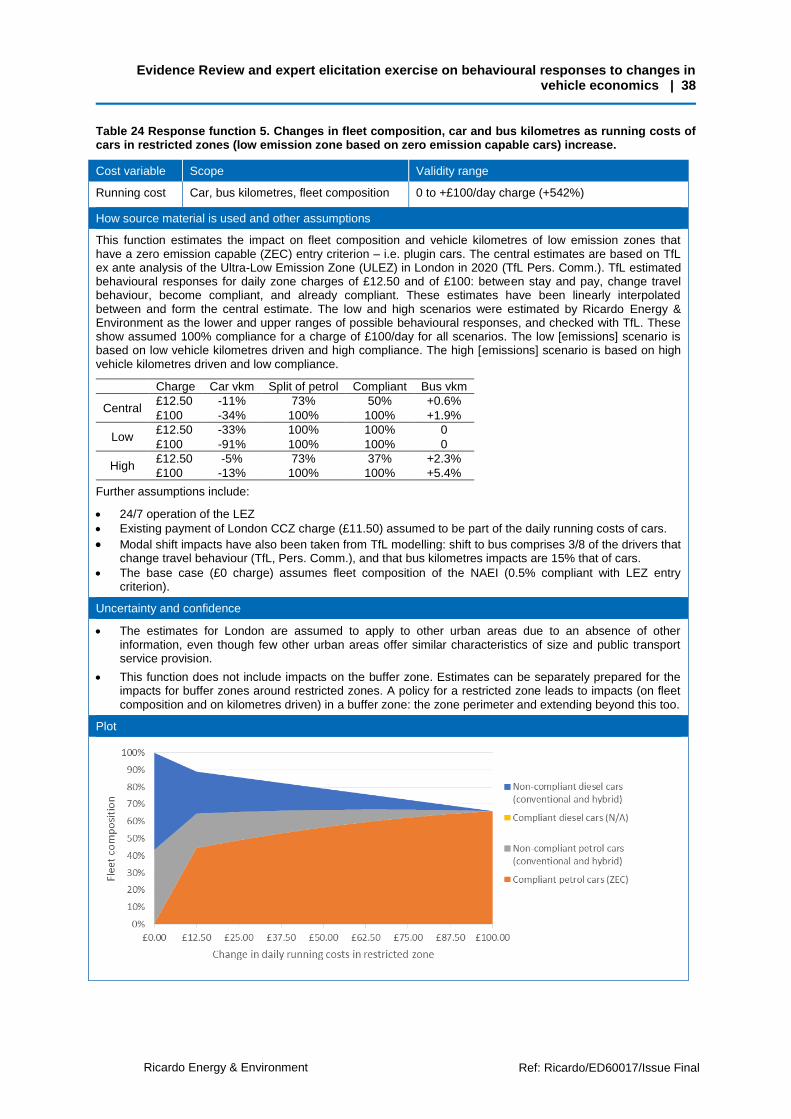
Evidence Review and expert elicitation exercise on behavioural responses to changes in vehicle economics | 38
Ricardo Energy & Environment Ref: Ricardo/ED60017/Issue Final
Table 24 Response function 5. Changes in fleet composition, car and bus kilometres as running costs of cars in restricted zones (low emission zone based on zero emission capable cars) increase.
Cost variable Scope Validity range
Running cost Car, bus kilometres, fleet composition 0 to +£100/day charge (+542%)
How source material is used and other assumptions
This function estimates the impact on fleet composition and vehicle kilometres of low emission zones that have a zero emission capable (ZEC) entry criterion – i.e. plugin cars. The central estimates are based on TfL ex ante analysis of the Ultra-Low Emission Zone (ULEZ) in London in 2020 (TfL Pers. Comm.). TfL estimated behavioural responses for daily zone charges of £12.50 and of £100: between stay and pay, change travel behaviour, become compliant, and already compliant. These estimates have been linearly interpolated between and form the central estimate. The low and high scenarios were estimated by Ricardo Energy & Environment as the lower and upper ranges of possible behavioural responses, and checked with TfL. These show assumed 100% compliance for a charge of £100/day for all scenarios. The low [emissions] scenario is based on low vehicle kilometres driven and high compliance. The high [emissions] scenario is based on high vehicle kilometres driven and low compliance.
Charge Car vkm Split of petrol Compliant Bus vkm
Central £12.50 -11% 73% 50% +0.6%
£100 -34% 100% 100% +1.9%
Low £12.50 -33% 100% 100% 0
£100 -91% 100% 100% 0
High £12.50 -5% 73% 37% +2.3%
£100 -13% 100% 100% +5.4%
Further assumptions include:
24/7 operation of the LEZ
Existing payment of London CCZ charge (£11.50) assumed to be part of the daily running costs of cars.
Modal shift impacts have also been taken from TfL modelling: shift to bus comprises 3/8 of the drivers that change travel behaviour (TfL, Pers. Comm.), and that bus kilometres impacts are 15% that of cars.
The base case (£0 charge) assumes fleet composition of the NAEI (0.5% compliant with LEZ entry criterion).
Uncertainty and confidence
The estimates for London are assumed to apply to other urban areas due to an absence of other information, even though few other urban areas offer similar characteristics of size and public transport service provision.
This function does not include impacts on the buffer zone. Estimates can be separately prepared for the impacts for buffer zones around restricted zones. A policy for a restricted zone leads to impacts (on fleet composition and on kilometres driven) in a buffer zone: the zone perimeter and extending beyond this too.
Plot

Evidence Review and expert elicitation exercise on behavioural responses to changes in vehicle economics | 39
Ricardo Energy & Environment Ref: Ricardo/ED60017/Issue Final
4.3.6 Response functions developed for LGVs
Table 25 Response function 2: Switch from Euro 6 diesel LGVs to PHEVs/BEVs as upfront costs of PHEVs and BEVs decrease
Cost variable Scope Validity range
Upfront costs LGVs, Euro 6, fleet composition 0 to 20% reduction in PHEV/BEV purchase costs
How source material is used and other assumptions
Element Energy et al. (2013) indicates that £3000 is the subsidy necessary to achieve a high pathway uptake of PHEVs/BEVs for LGVs and cars and that a £2000 subsidy produces half of this impact. (The pathway assumes there is still increased uptake of BEV/PHEVs without financial support, but it is not clear if this means without financial support beyond the existing subsidy regimes in place.) These absolute subsidies were expressed in percentage reductions of the base price of LGVs. The high uptake pathway is described in Element Energy et al. (2013) in terms of stock (numbers) of BEVs and PHEVs (cars and vans separately) for 2020. The numbers of LGVs and proportion they make up in the fleet were compared to existing business as usual projections in the NAEI and DfT stock data. The additional percentage of the fleet of BEV and PHEV (in terms of numbers) in Element Energy et al. (2013) compared to NAEI were added to the NAEI baseline fleet composition (in terms of vehicle kilometres).
The response function was estimated to have an upper range of validity of around 1.5 times the £3000 subsidy level. The function was extrapolated from the £0, £2000 and £3000 data points using an average of exponential and polynomial lines of best fit.
The following assumptions were made to produce this response function:
Existing purchase behaviour is switched, i.e. additional purchases are not encouraged. Total kilometres driven are therefore fixed – implicitly, the switched (new) vehicles are driven fleet average annual distances.
Petrol LGVs are ignored as they are projected in 2020 to make up only 1% of LGV kilometres travelled.
There is no impact on the fleet composition of full hybrids, as the switches are assumed to be solely between diesel LGVs and plugin LGVs.
As the function is associated with purchase of LGVs in the timeframe to 2020, only Euro 6 LGVs are affected; nil impact is assumed on the pre-Euro 6 LGV fleet.
Price parity with diesel LGV is estimated using projected 2020 purchase prices of plugin vans (Element Energy et al. 2013).
Uncertainty and confidence
Projected prices and resale prices of plugin LGVs for 2020 and hence level of price parity with diesel LGVs is highly uncertain. Resale values are most likely to have largest impact on fleet purchases. The market for EV and PHEV LGVs is much less well developed than for cars: there are very few vehicles of this nature on the market at the moment. This uncertainty is accounted for by varying the percentage fleet composition of plugins in 2020 by +/-50% in the high/low uncertainty bounds respectively.
Plot
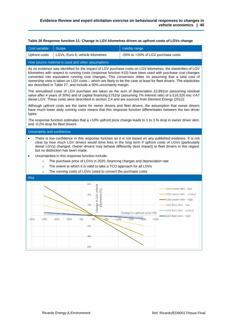
Evidence Review and expert elicitation exercise on behavioural responses to changes in vehicle economics | 40
Ricardo Energy & Environment Ref: Ricardo/ED60017/Issue Final
Table 26 Response function 11: Change in LGV kilometres driven as upfront costs of LGVs change
Cost variable Scope Validity range
Upfront costs LGVs, Euro 6, vehicle kilometres -20% to +20% of LGV purchase costs
How source material is used and other assumptions
As no evidence was identified for the impact of LGV purchase costs on LGV kilometres, the elasticities of LGV kilometres with respect to running costs (response function #10) have been used with purchase cost changes converted into equivalent running cost changes. This conversion relies on assuming that a total cost of ownership view is taken on LGV costs – which are likely to be the case at least for fleet drivers. The elasticities are described in Table 27, and include a 50% uncertainty margin.
The annualised costs of LGV purchase are taken as the sum of depreciation £2,891/yr (assuming residual value after 4 years of 30%) and of capital financing £752/yr (assuming 7% interest rate) of a £16,520 exc VAT diesel LGV. These costs were described in section 2.4 and are sourced from Element Energy (2012).
Although upfront costs are the same for owner drivers and fleet drivers, the assumption that owner drivers have much lower daily running costs means that this response function differentiates between the two driver types.
The response function estimates that a +10% upfront price change leads to 1 to 3 % drop in owner driver vkm, and -0.2% drop for fleet drivers.
Uncertainty and confidence
There is low confidence in this response function as it is not based on any published evidence. It is not clear by how much LGV drivers would drive less in the long term if upfront costs of LGVs (particularly diesel LGVs) changed. Owner drivers may behave differently (less impact) to fleet drivers in this regard, but no distinction has been made.
Uncertainties in this response function include:
o The purchase price of LGVs in 2020, financing charges and depreciation rate
o The extent to which it is valid to take a TCO approach for all LGVs
o The running costs of LGVs (used to convert the purchase costs
Plot

Evidence Review and expert elicitation exercise on behavioural responses to changes in vehicle economics | 41
Ricardo Energy & Environment Ref: Ricardo/ED60017/Issue Final
Table 27 Response function 10. Change in LGV kilometres driven as LGV running costs change
Cost variable Scope Validity range
Running costs Vehicle kilometres of all LGVs -50% to +50% of existing LGV running costs
How source material is used and other assumptions
Changes in LGV kilometres with respect to LGV running costs have been estimated using elasticities, drawing on expert panel suggestions of fuel cost elasticities: a low value of -0.1, a central value of -0.2 consistent with many literature estimates, including DfT; and a high value of -0.3. The central value has been selected on the basis of expert judgement that it should be lower than the accepted value for cars of -0.3. This is assumed to apply to all LGVs.
LGV owner drivers have been considered separately from LGV fleet drivers, as their cost bases are different.
No modal shift is assumed to other modes (cars, HGVs or buses / coaches) due to a lack of quantitative evidence although conceivably there could be shifts to all three other modes.
The validity range of the response function is assumed to be capped at changes of 50% of existing running costs. Daily LGV running costs were estimated and described in Table 2. Most notably, fuel costs were estimated to be around half of total running costs for owner drives. No changes are assumed in daily running costs for cars up to 2020.
Uncertainty and confidence
Confidence level is low and there is high uncertainty due to a lack of published literature on the behavioural responses.
Second order effects are ignored. For example, the effect of people tending to use vehicles with lower running costs more when running costs are increased is ignored. This is a rebound effect. It is unclear how large if any there would be in a shift to newer vehicles and/or different fuels
For owner-drivers, changes to perceived running costs (e.g. fuel) have higher impacts than to changes in costs that are often not accounted for by owner-drivers (e.g. fixed annual costs).
Plot
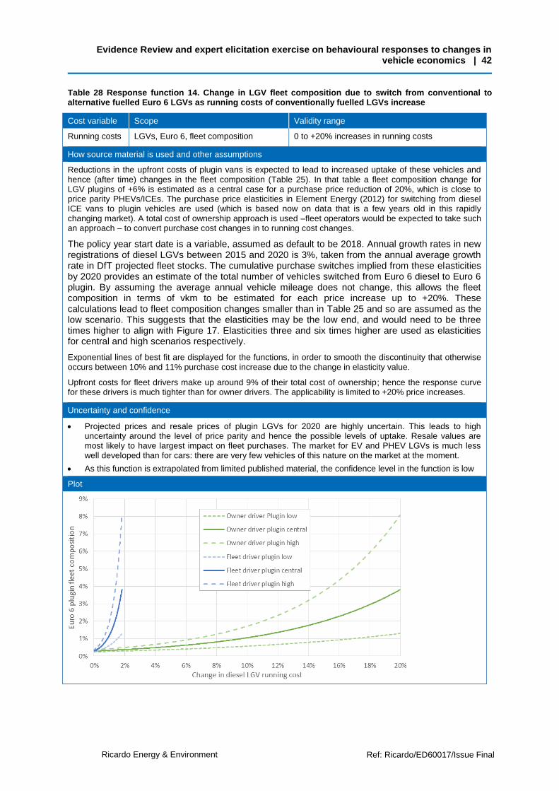
Evidence Review and expert elicitation exercise on behavioural responses to changes in vehicle economics | 42
Ricardo Energy & Environment Ref: Ricardo/ED60017/Issue Final
Table 28 Response function 14. Change in LGV fleet composition due to switch from conventional to alternative fuelled Euro 6 LGVs as running costs of conventionally fuelled LGVs increase
Cost variable Scope Validity range
Running costs LGVs, Euro 6, fleet composition 0 to +20% increases in running costs
How source material is used and other assumptions
Reductions in the upfront costs of plugin vans is expected to lead to increased uptake of these vehicles and hence (after time) changes in the fleet composition (Table 25). In that table a fleet composition change for LGV plugins of +6% is estimated as a central case for a purchase price reduction of 20%, which is close to price parity PHEVs/ICEs. The purchase price elasticities in Element Energy (2012) for switching from diesel ICE vans to plugin vehicles are used (which is based now on data that is a few years old in this rapidly changing market). A total cost of ownership approach is used –fleet operators would be expected to take such an approach – to convert purchase cost changes in to running cost changes.
The policy year start date is a variable, assumed as default to be 2018. Annual growth rates in new registrations of diesel LGVs between 2015 and 2020 is 3%, taken from the annual average growth rate in DfT projected fleet stocks. The cumulative purchase switches implied from these elasticities by 2020 provides an estimate of the total number of vehicles switched from Euro 6 diesel to Euro 6 plugin. By assuming the average annual vehicle mileage does not change, this allows the fleet composition in terms of vkm to be estimated for each price increase up to +20%. These calculations lead to fleet composition changes smaller than in Table 25 and so are assumed as the low scenario. This suggests that the elasticities may be the low end, and would need to be three times higher to align with Figure 17. Elasticities three and six times higher are used as elasticities for central and high scenarios respectively.
Exponential lines of best fit are displayed for the functions, in order to smooth the discontinuity that otherwise occurs between 10% and 11% purchase cost increase due to the change in elasticity value.
Upfront costs for fleet drivers make up around 9% of their total cost of ownership; hence the response curve for these drivers is much tighter than for owner drivers. The applicability is limited to +20% price increases.
Uncertainty and confidence
Projected prices and resale prices of plugin LGVs for 2020 are highly uncertain. This leads to high uncertainty around the level of price parity and hence the possible levels of uptake. Resale values are most likely to have largest impact on fleet purchases. The market for EV and PHEV LGVs is much less well developed than for cars: there are very few vehicles of this nature on the market at the moment.
As this function is extrapolated from limited published material, the confidence level in the function is low
Plot

Evidence Review and expert elicitation exercise on behavioural responses to changes in vehicle economics | 43
Ricardo Energy & Environment Ref: Ricardo/ED60017/Issue Final
Table 29 Response function 15. Changes in fleet composition, LGV and bus kilometres as running costs of LGVs in restricted zones (euro standard based low emission zone) increase.
Cost variable Scope Validity range
Running cost LGV, bus kilometres, fleet composition 0 to +£100/day charge (+453%/90% for owner/fleet drivers)
How source material is used and other assumptions
This function estimates the impact on fleet composition and LGV kilometres of low emission zones that have a Euro 6 diesel entry criterion. The central estimates are based on TfL ex ante analysis of the Ultra-Low Emission Zone (ULEZ) in London in 2020. TfL estimated behavioural responses for daily zone charges of £12.50 and of £100: between stay and pay, change travel behaviour, become compliant, and already compliant. These estimates have been linearly interpolated between and form the central estimate. The low and high scenarios were estimated by Ricardo Energy & Environment as the lower and upper ranges of possible behavioural responses, and checked with TfL. These show assumed 100% compliance for a charge of £100/day for all scenarios. The low [emissions] scenario is based on low vehicle kilometres driven and high compliance. The high [emissions] scenario is based on high vehicle kilometres driven and low compliance.
Charge LGV vkm Compliant Bus vkm
Central £12.50 -5% 90.4% +0.1%
£100 -11% 98.7% +0.2%
Low £12.50 -13% 100% 0
£100 -31% 100% 0
High £12.50 -2% 80.4% +0.4%
£100 -2% 98.7% +1.0%
Further assumptions include:
24/7 operation of the LEZ
Existing payment of London CCZ charge (£11.50) assumed to be part of the daily running costs
Modal shift impacts have also been taken from TfL modelling: shift to bus comprises 1/8 of the drivers that change travel behaviour (TfL, Pers. Comm.), and that bus kilometres impacts are 15% that of LGVs.
The base case (£0 charge) assumes fleet composition of the NAEI (69% compliant with LEZ entry criterion).
Petrol LGVs have been ignored as they are projected to be a very small part of the fleet
Uncertainty and confidence
The estimates for London are assumed to apply to other urban areas due to an absence of other information, even though few other urban areas offer similar characteristics of size and public transport service provision.
This function does not include impacts on the buffer zone. Estimates can be separately prepared for the impacts for buffer zones around restricted zones. A policy for a restricted zone leads to impacts (on fleet composition and on kilometres driven) in a buffer zone: the zone perimeter and extending beyond this too.
Plot [shown for central estimate, and as a function of owner driver running cost percentages]

Evidence Review and expert elicitation exercise on behavioural responses to changes in vehicle economics | 44
Ricardo Energy & Environment Ref: Ricardo/ED60017/Issue Final
Table 30 Response function 16. Changes in fleet composition, LGV and bus kilometres as running costs of LGVs in restricted zones (LEZ based on zero emission capable LGVs) increase.
Cost variable Scope Validity range
Running cost LGV, bus kilometres, fleet composition 0 to +£100/day charge (+453%/90% for owner/fleet drivers)
How source material is used and other assumptions
This function estimates the impact on fleet composition and LGV kilometres of low emission zones that have a zero emission capable (ZEC) entry criterion – i.e. plugin LGVs. The central estimates are based on TfL ex ante analysis of the Ultra-Low Emission Zone (ULEZ) in London in 2020. TfL estimated behavioural responses for daily zone charges of £12.50 and of £100: between stay and pay, change travel behaviour, become compliant, and already compliant. These estimates have been linearly interpolated between and form the central estimate. The low and high scenarios were estimated by Ricardo Energy & Environment as the lower and upper ranges of possible behavioural responses, and checked with TfL. These show assumed 100% compliance for a charge of £100/day for all scenarios. The low [emissions] scenario is based on low vehicle kilometres driven and high compliance. The high [emissions] scenario is based on high vehicle kilometres driven and low compliance.
Charge LGV vkm Compliant Bus vkm
Central £12.50 -10% 4% +0.1%
£100 -47% 64% +0.3%
Low £12.50 -32% 29% 0
£100 -77% 100% 0
High £12.50 -2% 0% +0.4%
£100 -37% 62% +1.0%
Further assumptions include:
24/7 operation of the LEZ
Existing payment of London CCZ charge (£11.50) assumed to be part of the daily running costs
Modal shift impacts have also been taken from TfL modelling: shift to bus comprises 1/8 of the drivers that change travel behaviour (TfL, Pers. Comm.), and that bus kilometres impacts are 15% that of LGVs.
The base case (£0 charge) assumes fleet composition of the NAEI (69% compliant with LEZ entry criterion).
Petrol LGVs have been ignored as they are projected to be a very small part of the fleet
Uncertainty and confidence
The estimates for London are assumed to apply to other urban areas due to an absence of other information, even though few other urban areas offer similar characteristics of size and public transport service provision.
This function does not include impacts on the buffer zone. Estimates can be separately prepared for the impacts for buffer zones around restricted zones. A policy for a restricted zone leads to impacts (on fleet composition and on kilometres driven) in a buffer zone: the zone perimeter and extending beyond this too.
Plot

Evidence Review and expert elicitation exercise on behavioural responses to changes in vehicle economics | 45
Ricardo Energy & Environment Ref: Ricardo/ED60017/Issue Final
4.3.7 Response functions developed for HGVs
Table 31 Response function 18: Change in HGV kilometres driven as upfront costs of HGVs change.
Cost variable Scope Validity range
Upfront costs Euro VI HGV vehicle kilometres -20% to +20% of HGV purchase costs
How source material is used and other assumptions
As no evidence was identified for the impact of HGV purchase costs on HGV kilometres, fleet composition or modal shift, the elasticities of HGV kilometres and impacts on rail freight with respect to running costs (described in Table 32) have been used with purchase cost changes converted into equivalent running cost changes.
This conversion relies on assuming that a total cost of ownership view is taken on HGV costs. The annualised costs of upfront HGV costs are taken as the sum of depreciation and of capital financing. These costs were described in section 2.4 and are primary derived from figures published by the Road Haulage Association. They are separately considered for rigid from articulated HGVs.
Only impacts on Euro VI HGVs are considered as only these vehicles can be affected by purchase decisions.
The function indicates a weak impact of purchase cost changes: +20% upfront price change is estimated to less than 1% drop in HGV vkm.
Uncertainty and confidence
No consideration is made for the distinction between diesel and gas HGVs. If a purchase price increase only affected gas trucks, then there may be no vkm impact as purchase decisions may switch to gas trucks.
Plot

Evidence Review and expert elicitation exercise on behavioural responses to changes in vehicle economics | 46
Ricardo Energy & Environment Ref: Ricardo/ED60017/Issue Final
Table 32 Response function 9: Change in HGV kilometres driven as HGV running costs change.
Cost variable Scope Validity range
Running costs Vehicle kilometres of all LGVs -26% to +26% of existing artic HGV running costs
-22% to +22% of existing rigid HGV running costs
How source material is used and other assumptions
Fuel price elasticities in the literature have been used to estimate the impact of changes in HGV daily running costs on HGV vkm:
High value of -0.84 (Graham and Glaister, 2004)
Central value of -0.15 (Whiteing, Pers. Comm.). This value was selected as the central value on the recommendation of expert panel member due to the focus specifically on running costs not total costs.
Low value of -0.15 (implied in Fowkes et al, 2010)
The high and the low elasticities serve as the uncertainty bounds.
Modal shift from road to rail has been accounted for in this function. Cross price elasticity of rail freight with respect to HGV running costs of +0.17, derived from Fowkes et al. (2010), was adopted for the central estimate (no other literature on cross elasticities were identified). The upper and lower bounds of uncertainty estimated using +/-50% on the central elasticity value. This is considered as a modal shift when in conjunction with the negative impact on HGV vkm.
The range of validity of the elasticities for running cost changes is taken from Fowkes et al. (2010) who assumed a perturbation equal to 74% increase in total cost of ownership. This has been translated into the increase for running costs only, separately for articulated and rigid HGVs. The +26% increase in daily running costs for articulated HGVs is equivalent to +£135/day and the +22% for rigid HGVs is equivalent to +£65/day.
No change in daily running costs for HGVs assumed up to 2020.
Uncertainty and confidence
Uncertainty around if or at what value threshold tipping points occur, leading to non-linear impacts not captured in this function; these depend on commodity.
There are many options available to operators to reduce running costs (improve vehicle loading, reduce empty running, routeing and scheduling, shift towards longer semi-trailers and double-deck trailers for those traffics that could benefit in terms of usable load space within GVW limits). The simple elasticity approach adopted is unlikely to accurately reflect the take up of these options. There is therefore high uncertainty with these response functions.
Rail freight estimates are based on limited evidence and so have high uncertainty.
Plot

Evidence Review and expert elicitation exercise on behavioural responses to changes in vehicle economics | 47
Ricardo Energy & Environment Ref: Ricardo/ED60017/Issue Final
Table 33 Response function 20: Changes in fleet composition, HGV kilometres and shift to rail as running costs of HGVs in restricted zones (euro standard based low emission zone) increase.
Cost variable Scope Validity range
Running cost HGV fleet composition, kilometres 0 to +£100/day charge (+34%/20% for rigid / articulated HGVs)
How source material is used and other assumptions
Fleet composition effects are estimated based on low emission zones that have a Euro VI entry criterion. The central estimates are based on TfL ex ante analysis of the Ultra-Low Emission Zone (ULEZ) in London in 2020. TfL estimated behavioural responses for daily zone charges of £100: stay and pay, change travel behaviour, become compliant, and already compliant. Impacts between no charge and £100 charge have been linearly interpolated between and form the central estimate. The low and high scenarios were estimated by Ricardo Energy & Environment as the lower and upper ranges of possible behavioural responses, and checked with TfL. The low [emissions] scenario is based on low vehicle kilometres driven and high compliance. The high [emissions] scenario is based on high vehicle kilometres driven and low compliance.
HGV vehicle kilometre impacts are estimated from implied elasticity in Fowkes et al. (2010) who modelled a lorry road user charging scheme implying an 84% increase in running costs, with HGV kilometre reductions of 16% (elasticity of -0.15). Upper and lower bounds of uncertainty were estimated using +/-50% on the central elasticity value. The upper range of validity of the perturbations is assumed to be as per Fowkes et al. (2010) who assumed a perturbation equal to 84% increase in running costs (although in practice is limited by the validity of the fleet composition impact validity. TfL’s estimate of predicted reductions in HGV kilometre within the London ULEZ of -2% at a charge value of £100 is on the lower bound of the range estimate.
Modal shift to rail is estimated using cross price elasticity of rail freight with respect to HGV running costs in restricted zones of +0.33 derived from Fowkes et al. (2010). This is adopted as the central value as the only evidence identified. Upper and lower bounds of uncertainty estimated using +/-50% on the central elasticity value. The upper range of validity of this elasticity is taken from Fowkes et al. (2010) who assumed a perturbation equal to 84% increase in running costs, equivalent to £430 for articulated HGVs and £295 for rigid HGVs.
Charge HGV vkm Compliant
Central £100 -4.5% rigids -3% artics
98%
Low £100 -6% rigids -4% artics
100%
High £100 -3% rigids -2% artics
83% rigids 94% artics
The LEZ is assumed to operate 24/7. The base case (£0 charge) assumes fleet composition of the NAEI (83% of rigid HGVs and 94% of articulated HGVs compliant with LEZ entry criterion).
Uncertainty and confidence
No published evidence was identified on real ex-post outcomes on HGV distances travelled (and fleet composition, modal shift) following introduction of a low emission zone. Consequently, the uncertainty in this response function is high.
Plot

Evidence Review and expert elicitation exercise on behavioural responses to changes in vehicle economics | 48
Ricardo Energy & Environment Ref: Ricardo/ED60017/Issue Final
4.3.8 Response functions developed for buses
Table 34 Response function 8: Change in bus kilometres, car kilometres and passenger rail demand as upfront costs of buses change.
Cost variable Scope Validity range
Upfront Bus, car kilometres -20% to +20% change in existing upfront bus costs
How source material is used and other assumptions
As no evidence was identified for the impact of bus purchase costs on bus kilometres, fleet composition or modal shift, the (low, central and high) elasticities of bus vkm, car vkm and passenger rail journey demand impacts with respect to bus running costs (described in Table 35) have been used with purchase cost changes converted into equivalent running cost changes.
This conversion relies on assuming that a total cost of ownership view is taken on bus costs. Upfront bus costs were described in section 2.4.
Uncertainty and confidence
The upper and lower uncertainty ranges are further widened for the upfront response functions by varying the assumed annual ownership cost by +/-50%.
This function is assumed to apply to buses and coaches, which is a simplification.
Plot
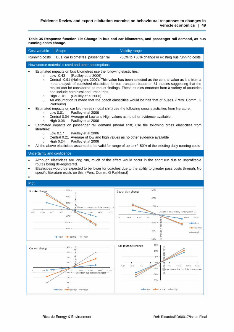
Evidence Review and expert elicitation exercise on behavioural responses to changes in vehicle economics | 49
Ricardo Energy & Environment Ref: Ricardo/ED60017/Issue Final
Table 35 Response function 19: Change in bus and car kilometres, and passenger rail demand, as bus running costs change.
Cost variable Scope Validity range
Running costs Bus, car kilometres, passenger rail -50% to +50% change in existing bus running costs
How source material is used and other assumptions
Estimated impacts on bus kilometres use the following elasticities: o Low -0.43 (Paulley et al 2006) o Central -0.91 (Holmgren, 2007). This value has been selected as the central value as it is from a
meta-analysis of published elasticities for bus transport based on 81 studies suggesting that the results can be considered as robust findings. These studies emanate from a variety of countries and include both rural and urban trips.
o High -1.01 (Paulley et al 2006) o An assumption is made that the coach elasticities would be half that of buses. (Pers. Comm. G
Parkhurst)
Estimated impacts on car kilometres (modal shift) use the following cross elasticities from literature: o Low 0.01 Paulley et al 2006 o Central 0.04 Average of Low and High values as no other evidence available. o High 0.06 Paulley et al 2006
Estimated impacts on passenger rail demand (modal shift) use the following cross elasticities from literature:
o Low 0.17 Paulley et al 2006 o Central 0.21 Average of low and high values as no other evidence available o High 0.24 Paulley et al 2006
All the above elasticities assumed to be valid for range of up to +/- 50% of the existing daily running costs
Uncertainty and confidence
Although elasticities are long run, much of the effect would occur in the short run due to unprofitable routes being de-registered.
Elasticities would be expected to be lower for coaches due to the ability to greater pass costs through. No specific literature exists on this. (Pers. Comm. G Parkhurst)
Plot

Evidence Review and expert elicitation exercise on behavioural responses to changes in vehicle economics | 50
Ricardo Energy & Environment Ref: Ricardo/ED60017/Issue Final
Table 36 Response function 17. Changes in fleet composition and bus kilometres as running costs of buses in restricted zones (Euro VI based low emission zone) increase
Cost variable Scope Validity range
Running costs Bus fleet composition and kilometres 0 to +£100/day additional running costs
How source material is used and other assumptions
The modelled predicted impacts of the London ULEZ (£100 charge, 24/7 applicability, charge applies to pre-Euro VI) on coaches are adopted as the predicted impacts for all restricted zones. These impacts are applied to buses and coaches.
A linear impact between £0 and £100 charge is assumed. No effects beyond £100/day are estimated.
Impacts on bus kilometres
The TfL modelling for the ULEZ assumed that 5% of coaches (and non-TfL buses) would stay and pay the charge, 9% would change their travel behaviour, and 19% would become compliant. The rest were already compliant in 2020. This behavioural response is associated with a predicted -4% vehicle kilometre reduction of these vehicles. This is adopted as the central estimate. The base case daily running cost associated with this is the assumed average UK value of £255/day.
The low estimate of vkm impacts is to assume that the behavioural response is instead 0% stay and pay, 33% change their travel behaviour, 0% become compliant (same remaining proportion already compliant). This is commensurate with assuming that peripheral zone coach transport hubs are exploited in preference to staying in zone and paying for compliance. This is an increase in the proportion of operators choosing to switch travel behaviour of (33/9), which multiplied by the -4% vkm effect in the central case leads to -15% vkm reduction estimated in the low case. The daily running cost here is assumed to be at the high end of the range (rest of UK, £263/day).
The high estimate of vkm impacts assumes zero impact in a zone, i.e. if all operators chose to stay and pay a charge. This could happen in case of the charge being small compared to existing costs or the ability to pass through the costs. The running cost is assumed to be at the low end of the range (London, £225).
Although the behavioural responses were modelled for coaches in London, further consultation with experts (Pers. Comm. G Parkhurst) indicates that the impacts on buses would fall within this range, although likely towards the upper end of the range (i.e. with small vkm effects assuming contracts would be renegotiated with local authorities) and towards the larger end for coaches. However, if LEZs were adopted across many urban areas, there may not be enough compliant buses to meet demand in the short term.
Impacts on fleet composition
The TfL modelling for the ULEZ assumed that the coach fleet composition would change in the following way with the introduction of the ULEZ £100 zone: Euro III drop from 2% to 0%, Euro IV drop from 5% to 1%, Euro V drop from 26% to 4% and Euro VI increase from 67% to 95%. This fleet composition change is adopted as the central case, adjusted to reflect NAEI average assumptions for buses and coaches.
The low estimate assumes that peripheral zone coach transport hubs are exploited in preference to compliance, such that within the zone, high levels of compliance occur (vkm effects taken account already in Figure 31), i.e. Euro VI is 100% of the fleet.
The high estimate, with no vkm change, assumes that no change to existing behaviour occurs, and there is no switch from the existing fleet mix.
Uncertainty and confidence
Within the range presented, effects for coaches are likely to be higher, and effects lower for buses. As coach operators are more likely to be able to pay charges for restricted zones, one would expect bus fleets within LEZs to be at the cleaner end of these ranges than coach fleets.
The emergence of low carbon technologies in buses and coaches is developing quite rapidly. Although not modelled, hybrid or inductive-charged electric buses could be used in LEZs. Capital costs are higher, but fuel and other running costs are lower. This effect is not accounted for.
Plot

Evidence Review and expert elicitation exercise on behavioural responses to changes in vehicle economics | 51
Ricardo Energy & Environment Ref: Ricardo/ED60017/Issue Final
5 References
ALLEN, J. & BROWNE, M. 2010. Road freight transport and sustainability in Britain 1984-2007. Report produced as part of the Green Logistics Project. Accessed from http://www.greenlogistics.org/themesandoutputs/wm9/downloads/Sustainablefreighttransport-nationalfinal.pdf
ASHBY, M. F. 2016. Chapter 10 - Case Study: Electric Cars. In: ASHBY, M. F. (ed.) Materials and Sustainable Development. Boston: Butterworth-Heinemann.
BALCOMBE, R., MACKETT, R., PAULLEY, N., PRESTON, J., SHIRES, J., TITHERIDGE, H., WARDMAN, M. & WHITE, P. 2004. The demand for public transport: a practical guide.
BOWEN, D. 2010. The London Congestion Charging Scheme: A Cost-Benefit Analysis. Duquesne University, Pennsylvania.
BRAND, C., ANABLE, J. & TRAN, M. 2013. Accelerating the transformation to a low carbon passenger transport system: The role of car purchase taxes, feebates, road taxes and scrappage incentives in the UK. Transportation Research Part A: Policy and Practice, 49, 132-148.
BRAND, C., TRAN, M. & ANABLE, J. 2012. The UK transport carbon model: An integrated life cycle approach to explore low carbon future. Energy Policy, 41, 107-124.
CAIRNS, S., SLOMAN, L., NEWSON, C., ANABLE, J., KIRKBRIDE, A. & GOODWIN, P. 2004. Smarter choices-changing the way we travel.
CLARK, P. & ALLSOP, R. 1993. The use of Stated Preference techniques to investigate likely responses to changes in workplace parking supply. Traffic engineering & control, 34.
DAHL, C. A. 2012. Measuring global gasoline and diesel price and income elasticities. Energy Policy, 41, 2-13.
DARGAY, J. M. & HANLY, M. 2002. The demand for local bus services in England. Journal of Transport Economics and Policy, 73-91.
DE JONG, G., SCHROTEN, A., VAN ESSEN, H., OTTEN, M. & BUCCI, P. 2010. Price sensitivity of European road freight transport–towards a better understanding of existing results. A report for Transport & Environment.
DEPARTMENT FOR TRANSPORT 2009. Revisiting the Elasticity Based Framework. Accessed from https://www.gov.uk/government/uploads/system/uploads/attachment_data/file/4227/rail-trends-report.pdf.
DEPARTMENT FOR TRANSPORT 2014a. TAG UNIT M2. Variable Demand Modelling. Accessed from: https://www.gov.uk/government/publications/webtag-tag-unit-m2-variable-demand-modelling
DEPARTMENT FOR TRANSPORT 2014b. Bus Statistics. Table BUS0103: Passenger journeys on local bus services by metropolitan area status and country: Great Britain, annual from 1970. Accessed from https://www.gov.uk/government/collections/bus-statistics
DEPARTMENT FOR TRANSPORT 2014c “Annex to the Low Emission HGV Task Force recommendations on the use of natural gas and biomethane in HGVs.” Accessed from: https://www.gov.uk/government/uploads/system/uploads/attachment_data/file/289185/annex-recommendations.pdf
EFTEC 2008. Demand for cars and their attributes. Final report for DfT. Accessed from http://www.eftec.co.uk/eftec-projects/demand-for-cars-and-their-attributes
ELEMENT ENERGY 2012. Ultra Low Emission Vans study Final Report. Accessed from: http://www.element-energy.co.uk/wordpress/wp-content/uploads/2012/05/Ultra-low-emission-vans-study_2012.pdf
ELEMENT ENERGY, ECOLANE & UNIVERSITY OF ABERDEEN 2013. Pathways to high penetration of electric vehicles.

Evidence Review and expert elicitation exercise on behavioural responses to changes in vehicle economics | 52
Ricardo Energy & Environment Ref: Ricardo/ED60017/Issue Final
EST 2012. Plugged in fleets – A guide to deploying electric vehicles in fleets Report by The Climate Group, CENEX and The Energy Saving Trust. Report by The Climate Group, CENEX and The Energy Saving Trust. Accessed from http://www.theclimategroup.org/what-we-do/publications/plugged-in-fleets-a-guide-to-deploying-electric-vehicles-in-fleets/
FEENEY, B. P. 1989. A review of the impact of parking policy measures on travel demand. Transportation Planning and Technology, 13, 229-244.
FOWKES, T., JOHNSON, D. & WHITEING, T. Modelling the Effects of Policies to Reduce the Environmental Impact of Freight Traffic in Great Britain. European Transport Conference, 2010, 2010.
GLAISTER, S., GRAHAM, D. & ASSOCIATION, U. K. P. I. 2000. The effect of fuel prices on motorists, AA Motoring Policy Unit Basingstoke.
GOODWIN, P. 2002. Are fuel prices important? Chapter 5 in Lyons, G., Chatterjee, K.,(2002). Transport Lessons from the Fuel Tax Protests of 2000.
GOODWIN, P. 2008. Policy incentives to change behaviour in passenger transport. May-2008.[Online]. Available: http://www. internationaltransportforum. org.[Accessed: 14-Dec-2012].
GOODWIN, P., CAIRNS, S., DARGAY, J., HANLY, M., PARKHURST, G., STOKES, G. & VYTHOULKAS, P. Changing Travel Behaviour. Presented at: ESRC Transport Studies Unit Final Conference, UK, 2004 UK. Accessed from http://eprints.ucl.ac.uk/1245/
GOODWIN, P., DARGAY, J. & HANLY, M. 2004. Elasticities of road traffic and fuel consumption with respect to price and income: a review. Transport reviews, 24, 275-292.
GOODWIN, P. B. 1992. A review of new demand elasticities with special reference to short and long run effects of price changes. Journal of transport economics and policy, 155-169.
GRAHAM, D. J. & GLAISTER, S. 2002. The demand for automobile fuel: a survey of elasticities. Journal of Transport Economics and policy, 1-25.
GRAHAM, D. J. & GLAISTER, S. 2004. Road traffic demand elasticity estimates: a review. Transport reviews, 24, 261-274.
GREEN FISCAL COMMISSION 2010. Reducing Carbon Emissions Through Transport Taxation. Accessed from: http://www.greenfiscalcommission.org.uk/images/uploads/gfcBriefing6_PDF_ISBN_v7.pdf
HENNESSY, H. & TOL, R. S. J. 2011. The impact of tax reform on new car purchases in Ireland. Energy Policy, 39, 7059-7067.
HILTON, D., CHARALAMBIDES, L., DEMARQUE, C., WAROQUIER, L. & RAUX, C. 2014. A tax can nudge: The impact of an environmentally motivated bonus/malus fiscal system on transport preferences. Journal of Economic Psychology, 42, 17-27.
HIVERT, L. 2013. Short-term break in the French love for diesel? Energy Policy, 54, 11-22.
HMRC HER MAJESTY'S REVENUE & CUSTOMS 2006. Report on the Evaluation of the Company Car Tax Reform: Stage 2.
HOLMGREN, J. 2007. Meta-analysis of public transport demand. Transportation Research Part A: Policy and Practice, 41, 1021-1035.
KING, D. A., GORDON, C. E. & PETERS, J. R. 2014. Does road pricing affect port freight activity: Recent evidence from the port of New York and New Jersey. Research in Transportation Economics, 44, 2-11.
LAJUNEN, A. 2014. Energy consumption and cost-benefit analysis of hybrid and electric city buses. Transportation Research Part C: Emerging Technologies, 38, 1-15.
LANE, B. & BANKS, N. 2010. LowCVP Car Buyer Survey: Improved environmental information for consumers. Accessed from http://www.lowcvp.org.uk/assets/reports/lowcvp-car-buyer-survey-2010-final-report-03-06-10-vfinal.pdf

Evidence Review and expert elicitation exercise on behavioural responses to changes in vehicle economics | 53
Ricardo Energy & Environment Ref: Ricardo/ED60017/Issue Final
LEAPE, J. 2006. The London congestion charge. The Journal of Economic Perspectives, 157-176.
LITMAN, T. 2013. Transport Elasticities: Impacts on Travel Behaviour. Accessed from, http://www.sutp.org/en-news/en-sutp-news/3506-transport-elasticities-impacts-on-travel-behaviour
LITMAN, T. 2013b. Understanding Transport Demands and Elasticities. How Prices and Other Factors Affect Travel Behaviour. Accessed from http://www.vtpi.org/elasticities.pdf
LUCAS, K. & LE VINE, S. 2009. The Car in British Society, Working Paper 2: Literature Review, RAC foundation. Accessed from http://www.racfoundation.org/assets/rac_foundation/content/downloadables/car%20in%20british%20society%20-%20lucas%20et%20al%20-%20170409%20-%20literature%20review%20wp2.pdf
MARSDEN, G. 2006. The evidence base for parking policies—a review. Transport policy, 13, 447-457.
MAYERES, I. & PROOST, S. 2013. The taxation of diesel cars in Belgium – revisited. Energy Policy, 54, 33-41.
METCALFE, R. & DOLAN, P. 2012. Behavioural economics and its implications for transport. Journal of Transport Geography, 24, 503-511.
PAULLEY, N., BALCOMBE, R., MACKETT, R., TITHERIDGE, H., PRESTON, J., WARDMAN, M., SHIRES, J. & WHITE, P. 2006. The demand for public transport: The effects of fares, quality of service, income and car ownership. Transport Policy, 13, 295-306.
POLEMIS, M. L. 2006. Empirical assessment of the determinants of road energy demand in Greece. Energy Economics, 28, 385-403.
PRUD’HOMME, R. & BOCAREJO, J. P. The London Congestion Charge: A Tentative Economic Appraisal. PIARC Seminar on Road Pricing with emphasis on Financing, Regulation and Equity 1/16 2005 Cancun, Mexico, 2005, April 11-13.
RAMIL, A. R. & GRAHAM, D. J. 2014. The demand for road transport diesel fuel in the UK: Empirical evidence from static and dynamic cointegration techniques. Transportation Research Part D 26, 60-66.
RAND EUROPE PREPARED FOR DEPARTMENT FOR TRANSPORT 2014. Road traffic demand elasticities: A rapid evidence assessment. Accessed from https://www.gov.uk/government/publications/road-traffic-demand-elasticities
REZVANI, Z., JANSSON, J. & BODIN, J. 2015. Advances in consumer electric vehicle adoption research: A review and research agenda. Transportation Research Part D: Transport and Environment, 34, 122-136.
RHA 2013. Cost tables. Accessed from http://www.rha.uk.net/docs/Cost%20Tables%202013.pdf
Ricardo-AEA (2012). “Opportunities to overcome the barriers to uptake of low emission technologies for each commercial vehicle duty cycle”. Report for the Task Force on Fuel Efficient, Low Emission HGV Technologies. Report number Ricardo-AEA/R/ED58189. Accessed from: http://www.ricardo-aea.com/cms/assets/Documents-for-Insight-pages/2.-Opportunities+for+low+emission+HGVs+-+final+report+2012-1.pdf
ROMILLY, P., SONG, H. & LIU, X. 1998. Modelling and forecasting car ownership in Britain: a cointegration and general to specific approach. Journal of Transport Economics and Policy, 165-185.
ROMILLY, P., SONG, H. & LIU, X. 2001. Car ownership and use in Britain: a comparison of the empirical results of alternative cointegration estimation methods and forecasts. Applied economics, 33, 1803-1818.
SANTOS, G. 2010. Introduction. Research in Transportation Economics, 28, 1.
SANTOS, G., BEHRENDT, H., MACONI, L., SHIRVANI, T. & TEYTELBOYM, A. 2010. Part I: Externalities and economic policies in road transport. Research in Transportation Economics,

Evidence Review and expert elicitation exercise on behavioural responses to changes in vehicle economics | 54
Ricardo Energy & Environment Ref: Ricardo/ED60017/Issue Final
28, 2-45.
SANTOS, G., BEHRENDT, H. & TEYTELBOYM, A. 2010. Part II: Policy instruments for sustainable road transport. Research in Transportation Economics, 28, 46-91.
SANTOS, G. & FRASER, G. 2006. Road pricing lessons from London. Economic Policy 21, 263–310.
SANTOS, G. & SHAFFER, B. 2004. Preliminary results of the London Congestion Charging Scheme. Public Works Management & Policy, 9, 164-181.
TANAKA, M., IDA, T., MURAKAMI, K. & FRIEDMAN, L. 2014. Consumers’ willingness to pay for alternative fuel vehicles: A comparative discrete choice analysis between the US and Japan. Transportation Research Part A: Policy and Practice, 70, 194-209.
TRANSPORT FOR LONDON TFL 2008. Demand Elasticities for Car Trips to Central London as revealed by the Central London Congestion Charge. Accessed from: http://www.tfl.gov.uk/cdn/static/cms/documents/demand-elasticities-for-car-trips-to-central-london.pdf
TRANSPORT FOR LONDON TFL 2011. Stricter emissions standards for central or inner London: a provisional assessment of potential feasibility and effectiveness. Available from: https://www.london.gov.uk/sites/default/files/Central%20and%20Inner%20London%20LEZ%20Feasibility%20Study.pdf
TRL 2010. Parking Measures and Policies Research Review. Accessed from: http://www.britishparking.co.uk/write/Documents/Library/Reports%20and%20research/parkingreport.pdf
TURCKSIN, L. & MACHARIS, C. Not Dated. Price Elasticity, Task 3.2, Part 1. Accessed from: http://www.belspo.be/belspo/ssd/science/Reports/CLEVER%20WP3.2%20Price%20elasticity.pdf
VICTORIA TRANSPORT POLICY INSTITUTE 2014. Online TDM Encyclopedia. Accessed from: http://www.vtpi.org/tdm/tdm12.htm
WHELAN, G. 2007. Modelling car ownership in Great Britain. Transportation Research Part A: Policy and Practice, 41, 205-219.
WHITEHEAD, J., FRANKLIN, J. P. & WASHINTON, S. 2014. The impact of a congestion pricing exemption on the demand for new energy efficiency vehicles in Stockholm. Transporation Research Part A: Policy and Practice, 70, 24-40.
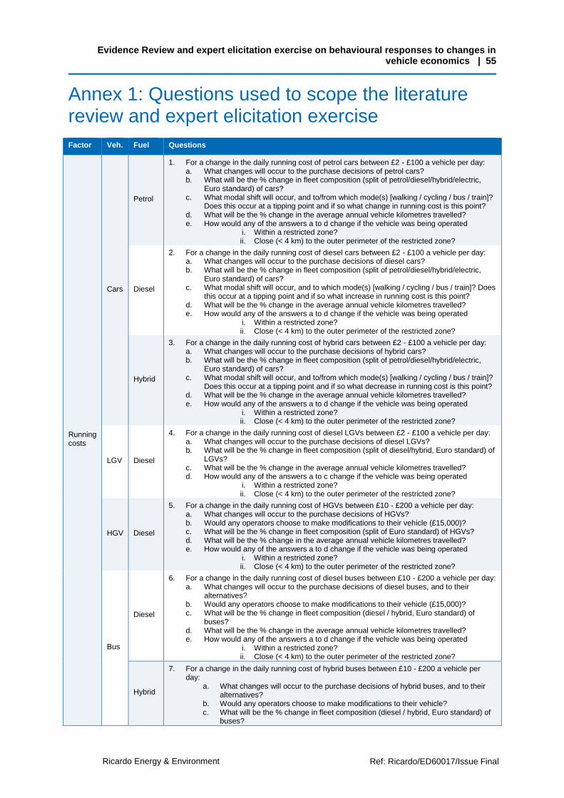
Evidence Review and expert elicitation exercise on behavioural responses to changes in vehicle economics | 55
Ricardo Energy & Environment Ref: Ricardo/ED60017/Issue Final
Annex 1: Questions used to scope the literature review and expert elicitation exercise
Factor Veh. Fuel Questions
Running costs
Cars
Petrol
1. For a change in the daily running cost of petrol cars between £2 - £100 a vehicle per day: a. What changes will occur to the purchase decisions of petrol cars? b. What will be the % change in fleet composition (split of petrol/diesel/hybrid/electric,
Euro standard) of cars? c. What modal shift will occur, and to/from which mode(s) [walking / cycling / bus / train]?
Does this occur at a tipping point and if so what change in running cost is this point? d. What will be the % change in the average annual vehicle kilometres travelled? e. How would any of the answers a to d change if the vehicle was being operated
i. Within a restricted zone? ii. Close (< 4 km) to the outer perimeter of the restricted zone?
Diesel
2. For a change in the daily running cost of diesel cars between £2 - £100 a vehicle per day: a. What changes will occur to the purchase decisions of diesel cars? b. What will be the % change in fleet composition (split of petrol/diesel/hybrid/electric,
Euro standard) of cars? c. What modal shift will occur, and to which mode(s) [walking / cycling / bus / train]? Does
this occur at a tipping point and if so what increase in running cost is this point? d. What will be the % change in the average annual vehicle kilometres travelled? e. How would any of the answers a to d change if the vehicle was being operated
i. Within a restricted zone? ii. Close (< 4 km) to the outer perimeter of the restricted zone?
Hybrid
3. For a change in the daily running cost of hybrid cars between £2 - £100 a vehicle per day: a. What changes will occur to the purchase decisions of hybrid cars? b. What will be the % change in fleet composition (split of petrol/diesel/hybrid/electric,
Euro standard) of cars? c. What modal shift will occur, and to/from which mode(s) [walking / cycling / bus / train]?
Does this occur at a tipping point and if so what decrease in running cost is this point? d. What will be the % change in the average annual vehicle kilometres travelled? e. How would any of the answers a to d change if the vehicle was being operated
i. Within a restricted zone? ii. Close (< 4 km) to the outer perimeter of the restricted zone?
LGV Diesel
4. For a change in the daily running cost of diesel LGVs between £2 - £100 a vehicle per day: a. What changes will occur to the purchase decisions of diesel LGVs? b. What will be the % change in fleet composition (split of diesel/hybrid, Euro standard) of
LGVs? c. What will be the % change in the average annual vehicle kilometres travelled? d. How would any of the answers a to c change if the vehicle was being operated
i. Within a restricted zone? ii. Close (< 4 km) to the outer perimeter of the restricted zone?
HGV Diesel
5. For a change in the daily running cost of HGVs between £10 - £200 a vehicle per day: a. What changes will occur to the purchase decisions of HGVs? b. Would any operators choose to make modifications to their vehicle (£15,000)? c. What will be the % change in fleet composition (split of Euro standard) of HGVs? d. What will be the % change in the average annual vehicle kilometres travelled? e. How would any of the answers a to d change if the vehicle was being operated
i. Within a restricted zone? ii. Close (< 4 km) to the outer perimeter of the restricted zone?
Bus
Diesel
6. For a change in the daily running cost of diesel buses between £10 - £200 a vehicle per day: a. What changes will occur to the purchase decisions of diesel buses, and to their
alternatives? b. Would any operators choose to make modifications to their vehicle (£15,000)? c. What will be the % change in fleet composition (diesel / hybrid, Euro standard) of
buses? d. What will be the % change in the average annual vehicle kilometres travelled? e. How would any of the answers a to d change if the vehicle was being operated
i. Within a restricted zone? ii. Close (< 4 km) to the outer perimeter of the restricted zone?
Hybrid
7. For a change in the daily running cost of hybrid buses between £10 - £200 a vehicle per day:
a. What changes will occur to the purchase decisions of hybrid buses, and to their alternatives?
b. Would any operators choose to make modifications to their vehicle? c. What will be the % change in fleet composition (diesel / hybrid, Euro standard) of
buses?

Evidence Review and expert elicitation exercise on behavioural responses to changes in vehicle economics | 56
Ricardo Energy & Environment Ref: Ricardo/ED60017/Issue Final
d. What will be the % change in the average annual vehicle kilometres travelled? e. How would any of the answers a to d change if the vehicle was being operated
i. Within a restricted zone? ii. Close (< 4 km) to the outer perimeter of the restricted zone?
Upfront costs
Cars
Petrol
8. For a change in the upfront cost of petrol cars of 2% to 20% (£400 – £4,000): a. What changes will occur to the purchase decisions of petrol cars? b. What will be the % change in fleet composition (split of
petrol/diesel/hybrid/electric, Euro standard) of cars? c. What modal shift will occur, and to/from which mode(s) [walking / cycling / bus /
train]? Does this occur at a tipping point and if so what change in upfront cost is this point?
d. What will be the % change in the average annual vehicle kilometres travelled?
Diesel
9. For a change in the upfront cost of diesel cars of 2% to 20% (£400 – £4,000): a. What changes will occur to the purchase decisions of diesel cars? b. What will be the % change in fleet composition (split of
petrol/diesel/hybrid/electric, Euro standard) of cars? c. What modal shift will occur, and to which mode(s) [walking / cycling / bus / train]?
Does this occur at a tipping point and if so what increase in upfront cost is this point?
d. What will be the % change in the average annual vehicle kilometres travelled?
Hybrid
10. For a change in the upfront cost of hybrid cars of 2% to 20% (£700 – £7,000): a. What changes will occur to the purchase decisions of hybrid cars? b. What will be the % change in fleet composition (split of
petrol/diesel/hybrid/electric, Euro standard) of cars? c. What modal shift will occur, and to/from which mode(s) [walking / cycling / bus /
train]? Does this occur at a tipping point and if so what decrease in upfront cost is this point?
d. What will be the % change in the average annual vehicle kilometres travelled?
Electric
11. For a change in the upfront purchase cost of electric cars of 2% to 20% (£700 – £7,000): a. What changes will occur to the purchase decisions of electric cars? b. What will be the % change in fleet composition (split of
petrol/diesel/hybrid/electric, Euro standard) of cars? c. What modal shift will occur, and to/from which mode(s) [walking / cycling / bus /
train]? Does this occur at a tipping point and if so what decrease in upfront cost is this point?
d. What will be the % change in the average annual vehicle kilometres travelled?
LGV Diesel
12. For a change in the upfront purchase cost of diesel LGVs of 2% to 20% (£400 – £4,000): a. What changes will occur to the purchase decisions of diesel LGVs? b. What will be the % change in fleet composition (split of diesel/hybrid, Euro
standard) of LGVs? c. What will be the % change in the average annual vehicle kilometres travelled?
HGV Diesel
13. For a change in the upfront purchase cost of HGVs of 2% to 20% (£1,400 – £14,000): a. What changes will occur to the purchase decisions of HGVs? b. What will be the % change in fleet composition (split of Euro standard) of HGVs? c. What will be the % change in the average annual vehicle kilometres travelled?
Bus
Diesel
14. For a change in the upfront purchase cost of diesel buses of 2% to 20% (£4,000 – £40,000): a. What changes will occur to the purchase decisions of diesel buses, and to their
alternatives? b. What will be the % change in fleet composition (diesel / hybrid, Euro standard) of
buses? c. What will be the % change in the average annual vehicle kilometres travelled?
Hybrid
15. For a change in the upfront purchase cost of hybrid buses of 2% to 20% (£6,000 – £60,000): a. What changes will occur to the purchase decisions of hybrid buses, and to their
alternatives? b. What will be the % change in fleet composition (diesel / hybrid, Euro standard) of
buses? c. What will be the % change in the average annual vehicle kilometres travelled?

Evidence Review and expert elicitation exercise on behavioural responses to changes in vehicle economics | 57
Ricardo Energy & Environment Ref: Ricardo/ED60017/Issue Final
Annex 2: Baseline vehicle costs
Assumptions for cars
Costs in Table 37 primarily sourced from the AA, averaging across size categories and fuel type:
http://www.theaa.com/resources/Documents/pdf/motoring-advice/running-costs/diesel2014.pdf
http://www.theaa.com/resources/Documents/pdf/motoring-advice/running-costs/petrol2014.pdf
Table 37 Assumed car costs
Cost Source
Upfront Financing £392 per year AA (2014)
Depreciation £2,615 per year AA (2014)
Running / Fixed
Insurance £500 per year AA (2014)
MOT £54 per year DVSA
Breakdown insurance £50 per year AA (2014)
VED £180 per year DVSA
Running / Variable
Fuel 13.6 pence per mile AA (2014)
tyres 2 pence per mile AA (2014)
Service labour 2.19 Pence per mile AA (2014)
Service parts 2.39 Pence per mile AA (2014)
Parking and tolls 2 pence per mile AA (2014)
Mileage 7900 Per year National Travel Survey 2013
Total running costs £6.95 Per day Totals of above
Total cost of ownership £15.19 Per day Totals of above
Assumptions for LGVs
Costs from a range of sources, shown in Table 38:
Table 38 Assumed LGV costs
Cost Source
Upfront Financing (4 years) £752 per year Element Energy (2012)
Depreciation (4 years) £2,891 per year Element Energy (2012)
Running / Fixed
Insurance - owner drivers £1,000 per year RHA (2013) minus goods in transit insurance estimated at £500/yr
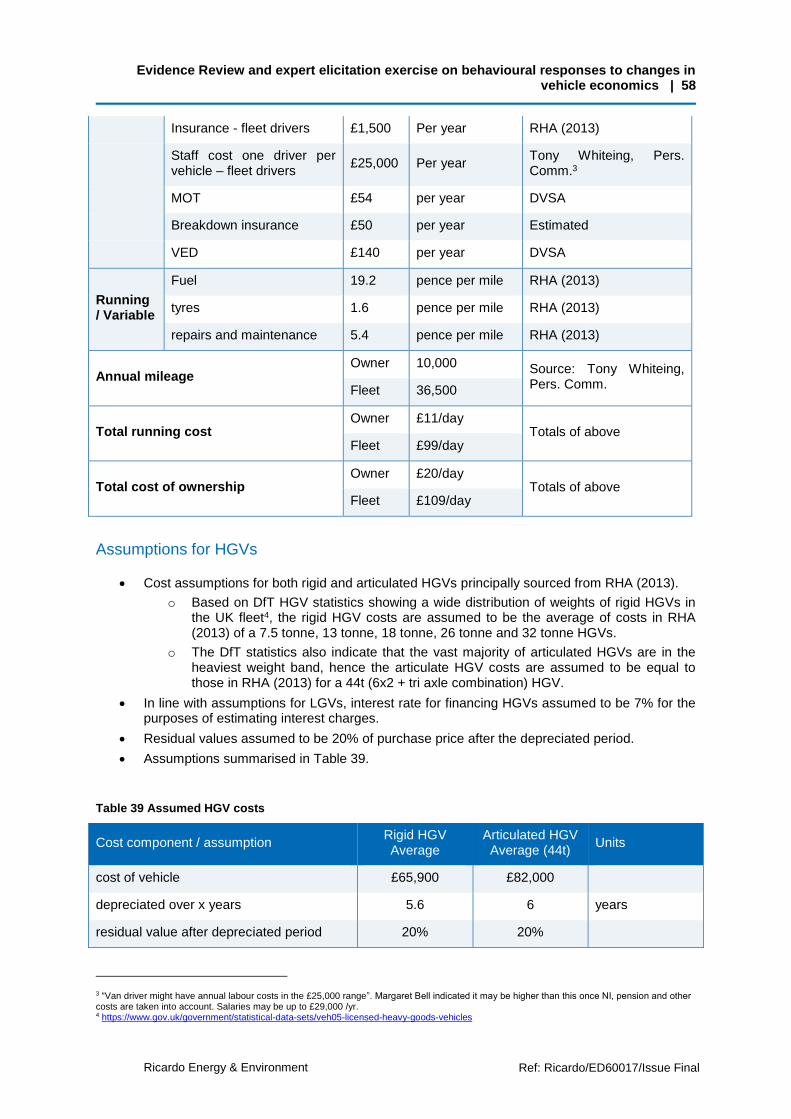
Evidence Review and expert elicitation exercise on behavioural responses to changes in vehicle economics | 58
Ricardo Energy & Environment Ref: Ricardo/ED60017/Issue Final
Insurance - fleet drivers £1,500 Per year RHA (2013)
Staff cost one driver per vehicle – fleet drivers
£25,000 Per year Tony Whiteing, Pers. Comm.3
MOT £54 per year DVSA
Breakdown insurance £50 per year Estimated
VED £140 per year DVSA
Running / Variable
Fuel 19.2 pence per mile RHA (2013)
tyres 1.6 pence per mile RHA (2013)
repairs and maintenance 5.4 pence per mile RHA (2013)
Annual mileage Owner 10,000 Source: Tony Whiteing,
Pers. Comm. Fleet 36,500
Total running cost Owner £11/day
Totals of above Fleet £99/day
Total cost of ownership Owner £20/day
Totals of above Fleet £109/day
Assumptions for HGVs
Cost assumptions for both rigid and articulated HGVs principally sourced from RHA (2013).
o Based on DfT HGV statistics showing a wide distribution of weights of rigid HGVs in the UK fleet4, the rigid HGV costs are assumed to be the average of costs in RHA (2013) of a 7.5 tonne, 13 tonne, 18 tonne, 26 tonne and 32 tonne HGVs.
o The DfT statistics also indicate that the vast majority of articulated HGVs are in the heaviest weight band, hence the articulate HGV costs are assumed to be equal to those in RHA (2013) for a 44t (6x2 + tri axle combination) HGV.
In line with assumptions for LGVs, interest rate for financing HGVs assumed to be 7% for the purposes of estimating interest charges.
Residual values assumed to be 20% of purchase price after the depreciated period.
Assumptions summarised in Table 39.
Table 39 Assumed HGV costs
Cost component / assumption Rigid HGV Average
Articulated HGV Average (44t)
Units
cost of vehicle £65,900 £82,000
depreciated over x years 5.6 6 years
residual value after depreciated period 20% 20%
3 “Van driver might have annual labour costs in the £25,000 range”. Margaret Bell indicated it may be higher than this once NI, pension and other costs are taken into account. Salaries may be up to £29,000 /yr. 4 https://www.gov.uk/government/statistical-data-sets/veh05-licensed-heavy-goods-vehicles

Evidence Review and expert elicitation exercise on behavioural responses to changes in vehicle economics | 59
Ricardo Energy & Environment Ref: Ricardo/ED60017/Issue Final
Depreciation £9,259 £10,933 per year
Interest on capital £2,768 £3,444 per year
Driver employment costs £28,840 £32,400 per year
Licenses £573 £1,200 per year
Vehicle insurance £2,640 £4,600 per year
Goods in transit insurance £324 £470 per year
Overheads £11,920 £28,430 per year
Fuel 44.9 64 ppm
tyres 3.9 5.9 ppm
repairs and maintenance 11.86 14.2 ppm
miles per annum 48000 71000
Days earning/yr 250 250
TCO £343 £565 Per day
% upfront 14% 9%
% running non fuel 61% 59%
% fuel 25% 32%
% total running 86% 91%
Assumptions for Buses and coaches
Total (operating and upfront) costs per day of £274 in London and £321 out of London; overall UK £311, based on £1.90/mile (source: DfT statistics), and annual distances of 53,000km/year in London and 62,000 km out of London (source: DfT statistics).
Daily running costs assumed to be 82% of this total figure, based on Confederation of Passenger Transport published data on bus operating costs.
So ownership costs can then be assumed to be £20,557/year.
Fuel costs derived to be £0.34/km, and average fuel efficiency of 6.3mpg. The fuel efficiency of coaches is likely to be higher than this.
No distinction made between coaches and buses of these costs. However it is recognised that TCO for coaches is likely to vary according to route (city / inter urban), mileage and MPG.

The Gemini Building Fermi Avenue Harwell Didcot Oxfordshire OX11 0QR United Kingdom
t: +44 (0)1235 753000 e: [email protected]
ee.ricardo.com