Embed Size (px)
Citation preview

Evaluation of Utility Pole Placement and the Impact on Crash Rates
A Thesis Report:
submitted to the Faculty
of the
WORCESTER POLYTECHNIC INSTITUTE
in partial fulfillment of the requirements for the
Degree of Master of Science
by
__________________
Amanda Gagne
Date: April 23, 2008
Approved:
___________________________________ ___________________________________
Professor Malcolm H. Ray, Major Advisor Professor Tahar El-Korchi, Department Head
___________________________________ ___________________________________
Professor Leonard D. Albano, Committee Member Professor Rajib B. Mallick, Committee Member

2
Abstract
Each year in the United States over 1,000 fatalities occur as a result of collisions with utility
poles. In addition, approximately 40% of utility pole crashes result in a non-fatal injury.
Moreover, with over 88 million utility poles lining United States highways, it is not feasible to
immediately remedy all poles that are potentially unsafe. Utility poles which pose a danger to
motorists can, however, be identified and addressed over time in a structured, methodical
manner. The goal of this project was to develop a method to identify and prioritize high risk
utility poles that are good candidates for remediation as well as develop a standard operating
procedure for the relocation of existing utility poles and placement of future utility poles along
Massachusetts highways. This research found that the lateral offset, annual average daily traffic
and density of the utility poles are major risk factors. Road geometry, however, also impacts the
risk. Basic corrective measures such as delineation, placing poles as far from the edge of road as
achievable, as well as placing poles a safe distance behind horizontal barriers are all suggested
solutions.

3
Acknowledgements
I would like to thank my advisor Professor Malcolm Ray for his suggestions, support and
guidance (and editing skills); Christine Conron and Chiara Silvestri for their assistance and
contributions, as well as my mother for her help and unceasing encouragement. I appreciate all
the knowledge, time, and effort that you have contributed. Thanks also to Mario Mongiardini for
his Matlab expertise, Mary Schultz for her assistance with data collection, Martin Bazinet for his
eternal optimism and to all my friends and family. I would also like to thank MassHighway for
their interest and cooperation.
4
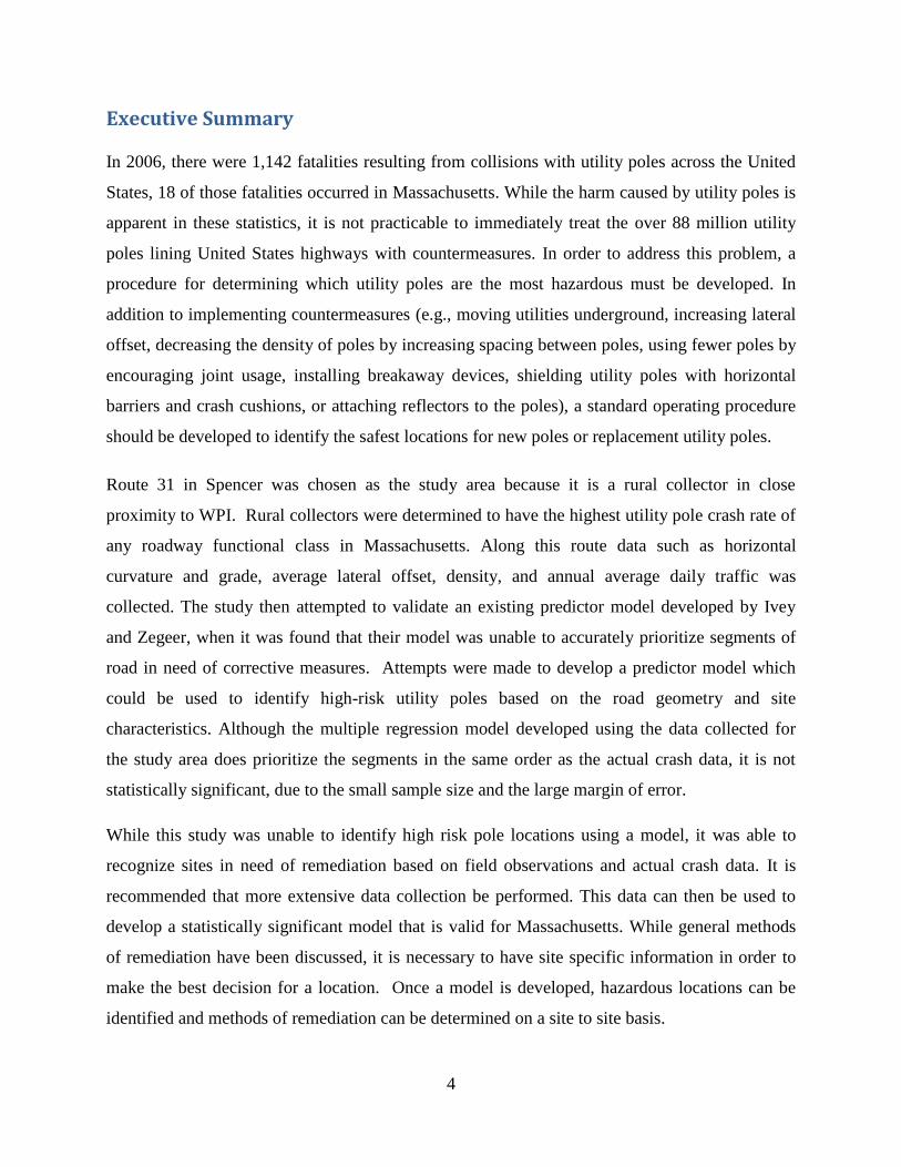
Executive Summary
In 2006, there were 1,142 fatalities resulting from collisions with utility poles across the United
States, 18 of those fatalities occurred in Massachusetts. While the harm caused by utility poles is
apparent in these statistics, it is not practicable to immediately treat the over 88 million utility
poles lining United States highways with countermeasures. In order to address this problem, a
procedure for determining which utility poles are the most hazardous must be developed. In
addition to implementing countermeasures (e.g., moving utilities underground, increasing lateral
offset, decreasing the density of poles by increasing spacing between poles, using fewer poles by
encouraging joint usage, installing breakaway devices, shielding utility poles with horizontal
barriers and crash cushions, or attaching reflectors to the poles), a standard operating procedure
should be developed to identify the safest locations for new poles or replacement utility poles.
Route 31 in Spencer was chosen as the study area because it is a rural collector in close
proximity to WPI. Rural collectors were determined to have the highest utility pole crash rate of
any roadway functional class in Massachusetts. Along this route data such as horizontal
curvature and grade, average lateral offset, density, and annual average daily traffic was
collected. The study then attempted to validate an existing predictor model developed by Ivey
and Zegeer, when it was found that their model was unable to accurately prioritize segments of
road in need of corrective measures. Attempts were made to develop a predictor model which
could be used to identify high-risk utility poles based on the road geometry and site
characteristics. Although the multiple regression model developed using the data collected for
the study area does prioritize the segments in the same order as the actual crash data, it is not
statistically significant, due to the small sample size and the large margin of error.
While this study was unable to identify high risk pole locations using a model, it was able to
recognize sites in need of remediation based on field observations and actual crash data. It is
recommended that more extensive data collection be performed. This data can then be used to
develop a statistically significant model that is valid for Massachusetts. While general methods
of remediation have been discussed, it is necessary to have site specific information in order to
make the best decision for a location. Once a model is developed, hazardous locations can be
identified and methods of remediation can be determined on a site to site basis.

5
Table of Contents
Abstract ........................................................................................................................................... 2
Acknowledgements ......................................................................................................................... 3
Executive Summary ........................................................................................................................ 4
Table of Contents ............................................................................................................................ 5
Table of Figures .............................................................................................................................. 7
1 Introduction ............................................................................................................................. 9
2 Background ........................................................................................................................... 12
2.1 AASHTO Roadside Design Guide (RDG)..................................................................... 12
2.2 Fox, Good, and Joubert .................................................................................................. 13
2.3 Mak and Mason .............................................................................................................. 16
2.4 Ivey and Zegeer .............................................................................................................. 27
2.5 Initiatives ........................................................................................................................ 29
2.5.1 Alabama .................................................................................................................. 29
2.5.2 New York ................................................................................................................ 32
2.5.3 Florida ..................................................................................................................... 34
2.5.4 Jacksonville Electric Authority ............................................................................... 34
2.5.5 Georgia .................................................................................................................... 35
2.5.6 Pennsylvania ........................................................................................................... 35
2.5.7 Washington State .................................................................................................... 36
2.5.8 Lafayette Utilities System ....................................................................................... 38
2.6 Steel Reinforced Safety Poles ........................................................................................ 38
2.7 Delineation ..................................................................................................................... 40
3 Methodology ......................................................................................................................... 41
3.1 Identification of a Study Area ........................................................................................ 41
3.2 Data collection................................................................................................................ 44
3.2.1 Stations .................................................................................................................... 45
3.2.2 Lateral Offset .......................................................................................................... 46
3.2.3 Density .................................................................................................................... 46
3.2.4 Annual Average Daily Traffic ................................................................................ 47
6
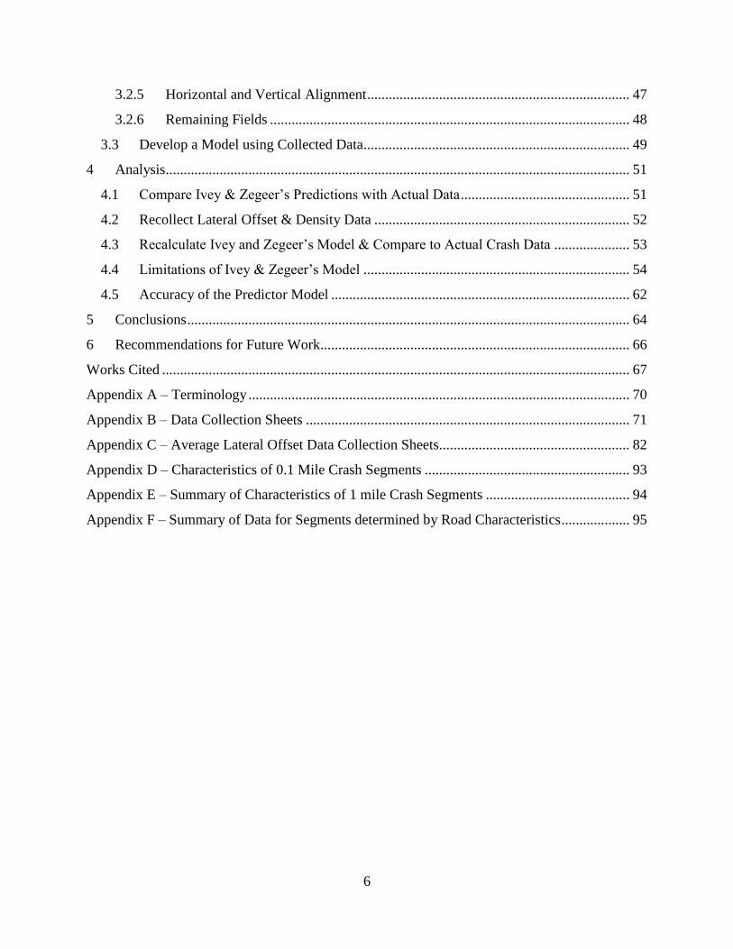
3.2.5 Horizontal and Vertical Alignment ......................................................................... 47
3.2.6 Remaining Fields .................................................................................................... 48
3.3 Develop a Model using Collected Data.......................................................................... 49
4 Analysis................................................................................................................................. 51
4.1 Compare Ivey & Zegeer‟s Predictions with Actual Data ............................................... 51
4.2 Recollect Lateral Offset & Density Data ....................................................................... 52
4.3 Recalculate Ivey and Zegeer‟s Model & Compare to Actual Crash Data ..................... 53
4.4 Limitations of Ivey & Zegeer‟s Model .......................................................................... 54
4.5 Accuracy of the Predictor Model ................................................................................... 62
5 Conclusions ........................................................................................................................... 64
6 Recommendations for Future Work...................................................................................... 66
Works Cited .................................................................................................................................. 67
Appendix A – Terminology .......................................................................................................... 70
Appendix B – Data Collection Sheets .......................................................................................... 71
Appendix C – Average Lateral Offset Data Collection Sheets..................................................... 82
Appendix D – Characteristics of 0.1 Mile Crash Segments ......................................................... 93
Appendix E – Summary of Characteristics of 1 mile Crash Segments ........................................ 94
Appendix F – Summary of Data for Segments determined by Road Characteristics ................... 95

7
Table of Figures Equation 1 ..................................................................................................................................... 15
Equation 2 ..................................................................................................................................... 15
Equation 3 ..................................................................................................................................... 16
Equation 4 ..................................................................................................................................... 18
Equation 5 ..................................................................................................................................... 21
Equation 6 ..................................................................................................................................... 22
Equation 7 ..................................................................................................................................... 28
Equation 8 ..................................................................................................................................... 37
Equation 9 ..................................................................................................................................... 42
Equation 10 ................................................................................................................................... 49
Table 1 - Summary of Regression Results for Rural Pole Accident Sites (12) ............................ 19
Table 2 - Summary of Regression Results for Urbanl Pole Accident Sites (12) .......................... 20
Table 2 - Accident distribution by highway type and type of roadway ........................................ 22
Table 3 - Distribution of Injury Severity by Type of Breakaway Device of Breakaway
Luminaries .................................................................................................................................... 25
Table 4 - Summary of NHTSA Accident Cost Estimates (in 1979 dollars) ................................. 27
Table 6 - Crash Rates by Roadway Functional Class ................................................................... 43
Table 6 – Actual Crash Data Priorities ......................................................................................... 51
Table 7 – Ivey & Zegeer‟s Predicted Priorities ............................................................................ 51
Table 8 – Comparison of Prioritized One-Mile Segments............................................................ 54
Table 9 - Common Characteristics of Stations with Crash History .............................................. 56
Table 10 - Prioritized Segments .................................................................................................... 62
Table 11 – Equation 9 Predicted Priorities ................................................................................... 63
Table 12 - Actual Crash Data Priorities ........................................................................................ 63
Figure 1 - Distribution of Fatal Fixed Object Crashes by Most Harmful Event (3) ....................... 9
Figure 2 - Utility pole struck by Ford Explorer (25) ...................................................................... 9
Figure 3 – Severe car collision with a utility pole (26) ................................................................... 9
Figure 4 - Car wrapped around a utility pole (27) ........................................................................ 10
Figure 5 – Utility pole after vehicle crashes into it (28) ............................................................... 10
Figure 6 - Distribution of Impact Speed for Non-intersection and Intersection Pole Accident Sites
....................................................................................................................................................... 23
Figure 7 - Distribution of Impact Speed for Urban and Rural Non-intersection Pole Accident
Sites ............................................................................................................................................... 23
Figure 8 - Relationship between Impact Speed, Velocity Change, and Momentum Change for
Utility Poles .................................................................................................................................. 24
Figure 9 - Relationship between Injury Rate and Impact Speed for Utility Poles ........................ 25
Figure 10 - Relationship between Injury Rate and Velocity Change for Utility Poles ................. 26
8
Figure 11 - Before Pole Relocation (23) ....................................................................................... 33
Figure 12 - After Pole Relocation (23) ......................................................................................... 33
Figure 13 - Number of Utility Pole Crashes in New York State from 1994-2006 (3) ................. 33
Figure 14 - TTI Model of a Ground Level Slip Base & Upper Hinge Assembly Prototype
Breakaway Utility Pole ................................................................................................................. 38
Figure 15 – Surveyor‟s Wheel a.k.a. Hodometer.......................................................................... 45
Figure 16 –Hodometer‟s measuring device .................................................................................. 45
Figure 17 – Electronic Distance Measuring Tool ......................................................................... 46
Figure 18 – Surveyor‟s Tape Measure .......................................................................................... 46
Figure 19 – A portion of the horizontal alignment and the aerial phtographs .............................. 48
Figure 20 – A portion of the vertical alignment ........................................................................... 48
Figure 21- Crashes per mile per year versus Lateral Offset ......................................................... 50
Figure 22- Crashes per mile per year versus Number of Poles per Mile ...................................... 50
Figure 23- Crashes per mile per year versus Grade ...................................................................... 50
Figure 24- Crashes per mile per year versus Horizontal Curvature.............................................. 50
Figure 25- Crashes per mile per year versus Posted Speed Limit ................................................ 50
Figure 26 - Pole located right behind guardrail ............................................................................ 53
Figure 27 – Guardrail ends before pole ........................................................................................ 53
Figure 28 - Station 00+00 North View ......................................................................................... 58
Figure 29 - Station 63+36 North View ......................................................................................... 58
Figure 30 - Station 184+80 North View ....................................................................................... 59
Figure 31 - Station 264+00 North View ....................................................................................... 59
Figure 32 - Station 322+08 North View ....................................................................................... 60
Figure 33 - Station 369+60 North View ....................................................................................... 60
Figure 34 - Station 417+12 North View ....................................................................................... 61
Figure 35 - Station 448+80 North View ....................................................................................... 61
Figure 36 - Station 469+92 North View ....................................................................................... 61
Figure 37 - Station 496+32 North View ....................................................................................... 61
Figure 38 - Two Poles Side by Side.............................................................................................. 65
Figure 39 – Remains of Hit Pole Left alongside Road ................................................................. 65

9
1 Introduction
In 2003, 44 percent of all fatal crashes
resulted from collisions with fixed
objects and non-collisions (e.g., fire,
submersion in bodies of water, etc.)
even though such crashes result in only
19 percent total of crashes. (1) Utility
pole collisions are the second most
frequent type of fatal fixed-object
crashes after trees (see Figure 1 which
shows impacting utility poles result in
12 percent of all fatalities resulting
from fixed object crashes, trees result
in the most fatalities at 48 percent).
Moreover, almost 40 percent of all crashes involving utility poles involve some type of non-fatal
injury. (2) Each year more than 1,000 deaths occur as a result of collisions with utility poles in
the United States alone. Last year 1,517 people were involved in 1,081 crashes in which the most
harmful event was a collision with a utility pole. These collisions resulted 1,071 fatal injuries (18
of which occurred in Massachusetts), 194 incapacitating injuries and 144 non-incapacitating but
evident injuries. (3) Shown below in Figure 2 and Figure 3 are examples of typical crashes with
utility poles. These images make clear the devastation resulting from colliding with a rigid,
unyielding structure like a utility pole.
Figure 3 – Severe car collision with a utility pole (26)
Figure 2 - Utility pole struck by Ford Explorer (25)
Figure 1 - Distribution of Fatal Fixed Object Crashes by Most
Harmful Event (3)

10
In recent years, fatalities associated with utility pole collisions have declined. With the widening
of many highways and streets, however, utility poles which were once outside the clear zones are
now much closer to the edge of pavement. (4) Moreover, with over 88 million utility poles
lining United States highways it is not feasible to immediately remediate all poles that are
potentially unsafe. Utility poles which pose a danger to motorists can, however, be identified and
addressed over time in a structured, methodical manner. (2) By remedying high risk locations,
crashes like those shown in Figure 4 and Figure 5 can potentially be avoided.
There have been numerous studies performed over the past three decades focused on reducing
the occurrence of fatalities due to collision with roadside fixed-objects. The three most
prominent studies include Mak & Mason‟s Accident Analysis - Breakaway and NonBreakaway
Poles Including Sign and Light Standards along Highways volume II - Technical Report
published in 1980, Fox, Good & Joubert‟s report entitled Collisions with Utility Poles performed
in Australia and released in 1979 and finally in 2004, the most recent report TRB State of the Art
Report 9 Utilities and Roadside Safety: Initiatives was published.
With this in mind, the goal of this project is to complete an In-Service Performance Evaluation
(ISPE) of utility poles along Massachusetts roadways. The purpose of conducting an ISPE is to
assess the functionality of a roadside device while in-service under actual traffic conditions. The
data collection standards for such a study are detailed in NCHRP Report 490. (5) In addition,
NCHRP Report 350(6) recommends that an ISPE is conducted using the following procedure:
1. Observe a minimum study period of two years,
Figure 5 – Utility pole after vehicle crashes into it (28)
Figure 4 - Car wrapped around a utility pole (27)
11
2. Study an adequate number of installations to obtain a statistically significant
collection of cases,
3. Perform several site visits,
4. Perform before and after accident studies,
5. Implement a method for monitoring unreported accidents,
6. Collect cost information for maintenance and repair and
7. Prepare a final report summarizing the evaluation.
Based upon the findings of the ISPE, a suggested policy for prioritization and remediation of
utility poles will be created which will be recommended to MassHighway for consideration of
implementation.

12
2 Background
Several studies have previously been conducted to investigate the relationship between the
placement of utility poles and the frequency of fatal crashes. Statistical models to calculate risk
have been created, methods of mitigating risk have been identified and initiatives have been
implemented in the hopes of reducing the occurrence and severity of utility pole-related crashes.
The following sections will review some of these previous studies as well as guidelines set forth
in the Roadside Design Guide. (7)
2.1 AASHTO Roadside Design Guide (RDG)
According to the 3rd
edition of the RDG released in 2006, crashes with utility poles result in ten
percent of all fatal fixed-object crashes. (7) This is a combined result of the quantity of poles in
use, their proximity to the edge of the road and their rigid nature. The RDG does not include
technical design details; it merely outlines alternatives for choosing a safe design. Below, listed
in order of preference, are options for providing a safer design:
1. Remove obstacle,
2. Redesign to allow safe navigation,
3. Relocation to point where object is less likely to be struck,
4. Reduce impact severity,
5. Shield obstacle or
6. Delineate obstacle.
Complicating the remediation effort is the fact that utility poles are generally privately owned
and are allowed on public rights of way, making it difficult for highway agencies to implement
corrective measures. Despite these complexities, RDG suggests that poles in new construction or
major reconstruction projects be placed as far from the edge of the traversable way as is
practical. Moreover, existing utility poles must be monitored to determine if there is a high
concentration of crashes at a particular location. Using crash records, high frequency crash
locations can be identified and analyzed. Based upon such analyses, recommendations can be
made and measures can be implemented to reduce both the severity and the frequency of crashes.
Countermeasures include:
Moving utilities underground,
Increasing lateral offset,

13
Decreasing the density of poles by increasing spacing between poles,
Using few poles by encouraging joint usage,
Installing breakaway devices,
Shielding utility poles with horizontal barriers and crash cushions, or
Attaching reflectors to the poles.
While relocating the utilities underground is the safest alternative for motorists, it is not always
feasible, in addition it is expensive to implement. Increasing offset and spacing as well as
combining usage decreases the frequency of crashes, whereas breakaway poles and shielding the
obstacles reduces the severity of the crash. In cases where none of the other measures are
implementable, delineation is a good option for reducing the risk of crashes occurring. Mainly,
the RDG stresses the forgiving roadside concept and describes basic ways of approaching
remediation. (7)
2.2 Fox, Good, and Joubert
According to Fox et al, in 1971, the Australian government ordered an assessment of the national
road system to understand the incidence and causation of highway crashes. One of the 24
resulting studies was performed by Good and Joubert which focused on accidents involving
fixed objects on the roadside and determining a strategy for the reduction of injuries and
fatalities. They found that available accident statistics were insufficient to meet the objectives of
their study in most Australian states. New South Wales, the only state with available suitable
data, reported that 2.2 percent of crashes were utility pole collisions yet they accounted for 7.5
percent of all road fatalities. Consequently, Good and Joubert recommended that the relationship
between utility pole crashes and road geometry, road type, traffic volume and location of the
pole be studied. In addition, they sought to determine whether specific pole locations are
particularly dangerous and identify the expense of relocating poles considered hazardous. A one
year study was undertaken to further investigate these relationships, both local and international
data was analyzed. Good and Joubert concluded that the available data was insufficient for such
an identification process using a „black-spot‟ method or risk predictor model. At the time no
relevant predictor model existed to describe the accidents. (8)
All available data relating to utility poles was summarized in a 1973 study by Wentworth, and he
also concluded that the existing data was inadequate. He recommended that warrants be

14
established for placing utilities underground or installing breakaway utility poles (note: at the
time frangible poles had not been designed). (9) In a subsequent study, Graf et al concluded that
inconsistent standards for the placement of utility poles and the legal inability of States to
implement corrective measures contribute to the difficulty of the problem. (10)
In 1976, Fox et al were commissioned to further explore utility pole collisions and their
contribution to the road accident situation. (11) The objectives of this study were to perform an
accident survey to gather more detailed information than regularly collected by accident reports
and then use this data to develop a statistical model able to predict the accident risk based upon
site characteristics. In addition, measures to reduce the harm resulting from utility pole accidents
would be examined. Finally, cost data was to be collected to develop a cost-benefit analysis.
Several in-field measurements were taken at arbitrarily selected utility pole sites. The „random‟
sample was then organized based on road class and whether or not it was located at an
intersection. Within these categories the concept of „relative risk‟ was used to develop a
statistical model to determine the accident involvement of poles with a specific characteristic
compared to the total population of utility poles. The model can assess the anticipated annual
crash rate for a specific site as a function of its site measurements.
The data necessary to evaluate the expected annual crash rate using the major road non-
intersection model includes:
1. Maximum horizontal curvature upstream of the pole.
2. Annual average daily traffic.
3. Pendulum skid test.
4. Lateral offset of pole.
5. Road width (only for undivided roads)
6. Distance between the pole and the start of the curve.
7. Pavement deficiencies (corrugations, etc.)
8. Super-elevation at curve.
9. Pole on the inside/outside of bend.
In view of the fact that all poles behave rigidly, no correlation was found between accident
occurrence and the pole material and function. These values, therefore, were not included in the
predictor model.

15
The best candidates for cost-effective remediation were poles along major non-intersection roads
and at major intersections. It was found that the instance of crashes at intersections was largely
dependent on the roadway characteristics rather than the pole characteristics. The controlling
variables were found to be:
1. Annual average daily traffic for both roads
2. Pendulum skid test.
3. Grade into the intersection.
4. Roads divided/undivided.
5. Lateral offset of the pole.
6. Intersection type.
Discerning the crash risk of one pole versus another is largely dependent upon the lateral offset
of the pole since it was found to be the only influential pole characteristic. (11)
The statistical analysis used the concept of “relative risk” to determine the crash risk of a pole
with particular attributes compared to the entire population of poles. The relative risk of a
specific characteristic is calculated using the following equation (Equation 1):
Relative risk plots and tables were created for several site attributes that were considered
predictor variables, Vi. These variables included lateral offset, pavement skid resistance, annual
average daily traffic, road width, super elevation, etc. The combined effect of risk variables is
computed using Equation 2:
Where RF is the risk factor which is the combined effects of the risk of predictor variables. MNI
stands for major non-intersection sites. The total relative risk (TRR) for a pole is obtained with
the following (Equation 3):
Equation 2
Equation 1
16
The relative risk associated with a data group when multiplied by the risk factor for that
particular group equals the total relative risk (TRR). Using the TRR and the mean crash
probability the expected number of pole accidents for a given site can be calculated. The mean
crash probability is deduced from an approximation of the total number of poles located in the
study area.
The study also evaluated methods of reducing the occurrence of crashes. Cost-benefit analysis
was performed and the researchers concluded that non-intersection poles along major roads have
the best prospects for cost-effective remediation. Intersections have the highest risk of accident
involvement; however, selective treatment of poles is not possible because variation is not
significant enough to make a distinction of risk. The approach used for remedial action of large
groups of poles must be evaluated on a site by site basis and the funds necessary to complete the
remediation must be included in the assessment.
In addition, recommendations were made to the Australian government for reducing risk through
the implementation of corrective action. The study suggests creating provision for funding
remedial programs and a policy to determine the cost of accidents. It also suggests that each
State compile data on the site characteristics of poles with a focus on the major roads and then
apply the predictor model to rank the sites and determine which are most in need of corrective
measures. Next, a site inspection should be performed to determine feasibility and site specific
requirements. A cost-benefit analysis should also be performed and the most beneficial
treatments should be implemented. Poles which were recognized by the study as “black spots”
or hazardous were to be immediately investigated and a treatment applied. Finally, a policy for
new installations was outlined.
2.3 Mak and Mason
In a study commissioned by the United States Department of Transportation, National Highway
Traffic Safety Administration (NHTSA) and Federal Highway Administration (FHWA), King K.
Equation 3
17
Mak and Robert L. Mason (12) performed an accident analysis of both breakaway and non-
breakaway poles along highways. The study was performed using data from 1976 to 1979.
The three primary stages of the study were: identifying the scope of the pole crash problem,
ascertaining the attributes of the roadway, vehicle and pole that relate to the characteristics of
pole crashes and finally, reviewing the performance of frangible and rigid metal poles. The
study utilized several sources to retrieve crash data including computerized crash data files, pole
crash reports, maintenance agency reports, scene inspection reports and in some cases even a
vehicle inspection, vehicle occupant interviews and medical records of crash victims. The study
consisted of seven study areas, investigated by five research teams. The study areas included:
1. Dallas, Texas
2. Nine counties in Kentucky and the city of Lexington
3. Los Angeles, Orange and Ventura counties in California
4. Bexar Country in Texas
5. Alameda, Contra Costa, Marin, San Francisco, San Mateo and Santa Clara counties in
California
6. Salt Lake City, Utah
7. Washington D.C.
The severe nature of pole crashes was the principal concentration of this study; the factors
influencing frequency were not as closely examined and evaluated. The study concluded that
pole crashes accounted for 3.3 percent of all reported crashes but contributed more significantly
in terms of severity. Pole crashes comprised 20.6 percent of all fatal crashes and 9.9 percent of
injury accidents. Utility poles were the most frequently struck object, however they were also
the most frequently occurring pole type on all highways. Collisions with rigid utility poles
resulted in the most severe injuries. In addition to utility poles, the study included sign supports,
luminaries, and traffic signal supports.
Not surprisingly, it was discovered that the closer a pole is placed to the roadway the more likely
it would be struck by an errant vehicle. Another characteristic of pole accident sites is they have
a much higher pole density than the average population. The impact of accident site
characteristics on the accident and injury severity is subtle, yet frequency of occurrence is related
to some of the attributes such as pole density and offset as well as horizontal and vertical

18
alignment. Using regression analysis the following equation was developed to predict crashes
based on the characteristics of the:
Equation 4
error term
equation theinto entered t variableindependen ofnumber
t variableindependenith for thet coefficien
constraint
t variableindependenith
variabledependent
where
0
22110
p
X
Y
XXXXY
i
i
ppii
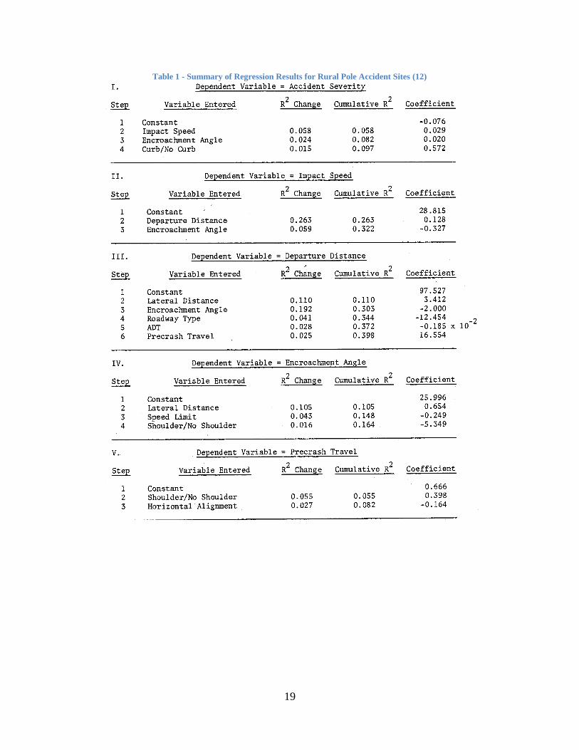
Two sets of coefficients were determined, one for rural pole accident sites (displayed in Table 1
on page 19) and another for urban pole accident sites (shown in Table 2 on page 20). The
relationship between these site characteristics and the risk of impact is not well defined because
of the lack of information regarding non-accident sites with which to compare data.
19
Table 1 - Summary of Regression Results for Rural Pole Accident Sites (12)

20
From the performance evaluation of breakaway and non-breakaway poles it was discovered that
frangible poles were successful in reducing the occurrence and severity of injuries in large posts
collisions such as those with large sign supports and luminaries. Small signs supports did not
benefit because of the already minor nature of accidents.
The cost-effectiveness was quantified using a basic benefit/cost ratio: the expected reduction in
accident costs by utilizing frangible poles is used to calculate effectiveness (benefit) and the
Table 2 - Summary of Regression Results for Urbanl Pole Accident Sites (12)
21
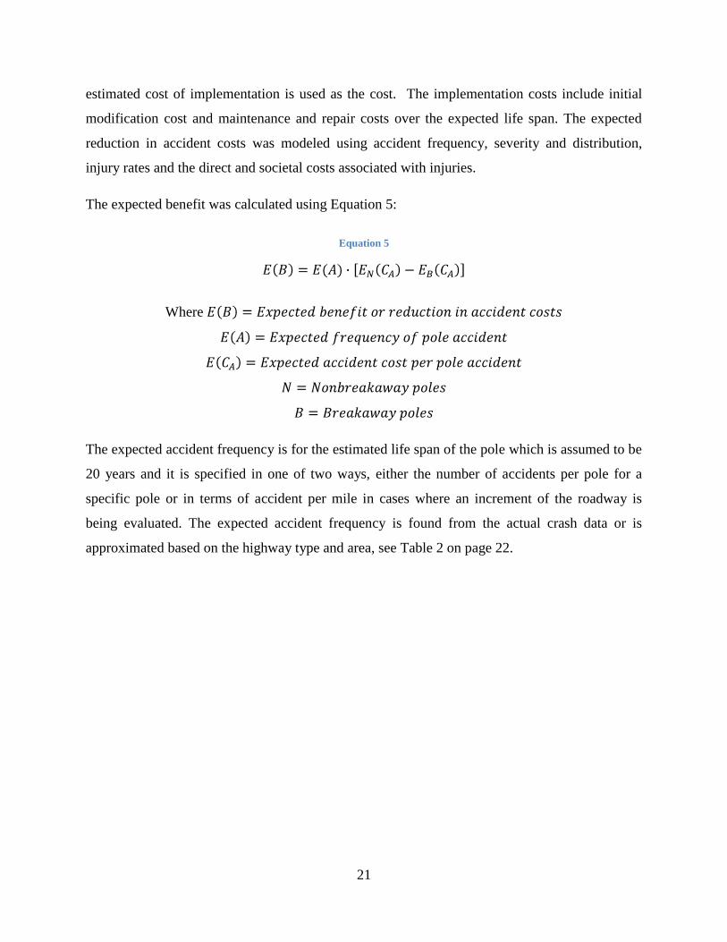
estimated cost of implementation is used as the cost. The implementation costs include initial
modification cost and maintenance and repair costs over the expected life span. The expected
reduction in accident costs was modeled using accident frequency, severity and distribution,
injury rates and the direct and societal costs associated with injuries.
The expected benefit was calculated using Equation 5:
Where
The expected accident frequency is for the estimated life span of the pole which is assumed to be
20 years and it is specified in one of two ways, either the number of accidents per pole for a
specific pole or in terms of accident per mile in cases where an increment of the roadway is
being evaluated. The expected accident frequency is found from the actual crash data or is
approximated based on the highway type and area, see Table 2 on page 22.
Equation 5
22
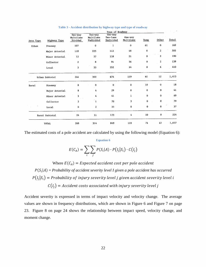
The estimated costs of a pole accident are calculated by using the following model (Equation 6):
Where
= Probability of accident severity level I given a pole accident has occurred
Accident severity is expressed in terms of impact velocity and velocity change. The average
values are shown in frequency distributions, which are shown in Figure 6 and Figure 7 on page
23. Figure 8 on page 24 shows the relationship between impact speed, velocity change, and
moment change.
Equation 6
Table 3 - Accident distribution by highway type and type of roadway

23
Figure 7 - Distribution of Impact Speed for Urban and Rural Non-intersection Pole Accident Sites
Figure 6 - Distribution of Impact Speed for Non-intersection and Intersection Pole Accident Sites

24
Figure 8 - Relationship between Impact Speed, Velocity Change, and Momentum Change for Utility Poles

25
The corresponding probability of an accident occurring at a specific speed can be ascertained
using Table 3.
The injury severity is expressed in terms of AIS which is the relationship between the injury rate
and the velocity change; this is displayed in Figure 9 and Figure 10.
Figure 9 - Relationship between Injury Rate and Impact Speed for Utility Poles
Table 4 - Distribution of Injury Severity by Type of Breakaway Device of Breakaway Luminaries

26
The accident cost includes both direct and indirect costs to society. Direct costs include medical
expenses, legal expenses, lost wages and work, property loss, etc. Indirect costs consist of
intangible costs such as pain and suffering and future production loss. The costs associated with
accidents are variable from one accident to another; therefore the study assumed the costs were
equal to the NHTSA cost estimates shown in Table 4.
Figure 10 - Relationship between Injury Rate and Velocity Change for Utility Poles

27
The study thoroughly examined the characteristics associated with pole accidents as well as the
scope of the pole problem and assessed the cost-effectiveness of remediation.
2.4 Ivey and Zegeer
In TRB State of the Art Report 9, Ivey and Zegeer identified and applied the strengths of
previously developed approaches when they created an approach for prioritizing and treating
hazardous utility poles. The main focus of any collision reduction program is maximizing the
benefit to society for every expense. (13) Moreover, the program should also provide state and
municipal departments with a strong defensive position in the event of litigation. This particular
study attempts to meet the following objectives while still meeting the economic and legal
constraints previously mentioned:
Table 5 - Summary of NHTSA Accident Cost Estimates (in 1979 dollars)
28
1. Prevent the occurrence of additional fatalities and injuries at site where collisions have
already taken place.
2. Identify sites where a fatal or injury-causing crash is likely to occur and prevent it.
3. Use fewer utility maintenance funds.
4. Place utilities where they are protected from a clearly random collision.
The approach developed to meet these goals consisted of three elements: the best offense, the
best bet and the best defense.
The best offense entails improving safety at sites where an unusual number of collisions have
already occurred. This applies directly to objective 1 and works toward 2, 3, and 4. Collision
information can be obtained from the appropriate law enforcement agency crash reports. At least
three years of accident data is suggested to determine the most vulnerable sites and perform
statistically relevant analysis. Poles or objects identified as hazardous can be prioritized for
remediation. The negative aspect of this approach is that it is reactive rather than proactive. This
approach will be important when the program is initially established but its importance will
diminish as more proactive measures are taken.
Best bet is the second phase of the approach which utilizes statistical algorithms to identify and
rank sites before collisions actually occur. There are several statistical relationships available for
performing analysis, including the ones developed by Mak and Mason and those developed by
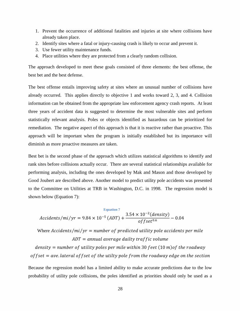
Good Joubert are described above. Another model to predict utility pole accidents was presented
to the Committee on Utilities at TRB in Washington, D.C. in 1998. The regression model is
shown below (Equation 7):
Where
Because the regression model has a limited ability to make accurate predictions due to the low
probability of utility pole collisions, the poles identified as priorities should only be used as a
Equation 7

29
guide, not the sole deciding factor when determining changes. If the model is used in
collaboration with road widening projects or right-of-way expansions it can be used to identify
sections that would benefit the most from acquisition of additional land or identify projects with
higher priory for remediation. This approach directly applies to Objective 2 and assists with 3
and 4.
Finally, the best defense approach addresses methods of reducing liability associated with
structures that fail to meet the standards suggested by the Roadside Design Guide. (7)
Recommended ways of reducing liability exposure are:
Document the placement of objects within the restricted zone against the
recommendations of the RDG.
Determine the percent compliance (PC) of these objects based on their physical
characteristics. Based on the PC determine a priority number (PN). The relationship
between the PC and PN is used to determine the most productive priority listing of sites.
Plan remediation of sites using the priority number.
Treat sufficient number of the highest priority sites each year.
By tracking the percent compliance of an area and ranking it in this manner, records will show
that the area was a low priority for treatment; therefore if the site experiences an unpredictable
random collision, there is a documented and sound defensive position. This meets objective 4.
(13)
2.5 Initiatives Several states and utility companies have implemented programs for reducing the number and
severity of crashes involving utility objects. Outlined below are several of these programs.
2.5.1 Alabama
In 2003, the state of Alabama adopted a goal of reducing crashes, injuries, and fatalities by 20
percent over the next ten years. (14) In an effort to realize this goal, a study was performed to
determine the impact a reduction of utility pole related crashes would have on overall roadside
safety. The study was performed using utility pole related crash data collected between 1996 and
2000.
The study used the Crash Analysis Reporting Environment (CARE) program to gather and
examine pole related crash data in Alabama for the five year study period. From this analysis,
researchers determined utility pole crashes comprise only one percent of all accidents however

30
2.4 percent of all fatalities resulted from these crashes. Moreover, utility pole crashes along state
controlled highways appear to pose a greater problem than non-state controlled roads, since 2.1
percent of utility pole related crashes on state controlled highways were fatal as compared with
1.1 percent on non-state controlled roads. In addition, the researchers attempted to determine if
utility pole accidents were simply random events or if they were clustered or located along
segments of utility pole lines. In order to determine if events were related, mile marked roads
were examined in five mile increments to see if more than one fatality occurred in any five mile
segment. All roads that were not marked by mile markers were studied along different stretches
of varying lengths to determine if more than one fatality occurred. Finally, all intersections were
examined to discover if more than one fatality had occurred at a given intersection.
Researchers found that no state-controlled intersection or roadway had more than one fatal utility
pole crash during the five year study period. Only one five mile segment of road had more than
one fatal crash, and the two crashes were 3.6 miles apart. From this researchers reasoned that
there were no closely related fatal crashes, and in Alabama fatal crashes involving utility poles
are relatively random events. While this was the finding of the research team, this statement may
be ill considered; although the study did not identify a relationship between fatal crashes in the
five mile segments studied it doesn‟t mean that none exists rather that they were simply unable to
detect a link.
Instead of basing potential remediation site selection on crash severity, the total number of
crashes was used to identify sites. For intersections the criteria for further investigation were
intersections with three or more crashes in four years, this yielded nine intersections. Along non-
mile marked segments sites with four or more crashes in four years were identified for further
study; this consisted of nine segments of road. Finally, five mile increments of mile-marked
roads with more than two crashes in three years were identified; severity was not considered.
The search produced 126 segments of roadway with a minimum of two crashes in three years.
The number was narrowed for further study using a severity method to evaluate them; all crashes
were converted to property-damage-only (PDO) equivalents. Fatal crashes equaled 10 PDO
crashes and one injury crashes had a PDO equivalent of three. Nineteen sites with PDO
equivalents greater than 10 were selected for further study. Of the 37 sites identified, 11 of these
sites were determined to be impacts with luminaries, not utility poles, and an additional site
31
could not be located because the milepost given in the computer database was not found in the
field, therefore 25 sites were chosen for site visits.
Students from the University of Alabama performed the site investigations, photographs of the
utility pole were taken and Utility Pole Accident Site Report Forms were completed. Based on
the field investigations, the following observations were made: in urban sites it is unlikely that
poles can be relocated, in rural sites poles were already 25 to 50 feet from the road, many sites
would be expensive to relocate because they were connected to high-cost or ancillary devices,
and several poles were not owned by utilities but rather by municipalities. Based on the
information collected, the Advisory Committee estimated that 50 percent of yearly pole-related
crashes could be avoided by remediation of approximately 20 crashes per year. This was only
0.015 percent of all crashes in Alabama each year, therefore, the Advisory Committee expressed
concern that the implementation of a remediation plan for these sites would not be cost-effective
given its minor impact on the overall roadside safety.
The possibility of these sites competing for funds in existing remediation programs such as the
Hazard Elimination (HES) program was evaluated and only one site could be considered for the
HES program, moreover it would have a difficult time competing for funds. Based on this, the
list of 25 sites was reviewed again to determine if any would be good candidates for remediation.
Sites that would be too difficult to treat as well as sites where the poles were already located 25
to 50 feet from the road or at the edge of the right of way line were immediately discarded. In
the end five sites were identified for treatment in future construction projects.
The research team also drafted a policy that potentially could be adopted by Alabama
Department of Transportation (ALDOT). It outlines the following for managing poles involved
in multiple crashes:
Encourage collaboration between ALDOT and utility companies during the permitting
process to ensure a clear zone is provided.
Periodically perform utility pole-related crash analysis as a part of the yearly crash
analysis study. The analysis should consider crash history, crash potential and cost
effectiveness when determining the method of remediation.
ALDOT should perform an in-field investigation of any site that experiences a fatal crash
in addition to another crash, two or more injury crashes, or four or more total crashes
within a three year period.

32
If a site is determined to require further investigation, the pole owner and users should be
notified of the situation, and the appropriate parties should evaluate the site to decide the
feasibility of remediation.
Finally, if an ALDOT construction project is scheduled to begin within two years from
the date of the site visit, treatment of the pole should be included in the project.
ALDOT and utility personnel will evaluate the site and identify feasible treatments. These
methods will be submitted to the Multimodal Transportation Bureau for review to determine the
most cost efficient and beneficial method of remediation. (14)
2.5.2 New York
Prompted by over 8,000 utility pole-related crashes, which resulted in over 100 fatalities and
about 6,600 injuries in the course of one year, New York began its utility pole safety program in
1982. (14)
Sites were prioritized using accident frequency and severity, and the accident data was obtained
from the State Accident Surveillance System. (15) In order to identify “bad actors,” the state
tracked utility pole crashes during a seven-year period along 0.1 mile roadway segments.
Segments with five or more crashes or a fatal crash in addition to another crash in the seven year
study period were deemed “bad actors.” “Bad actors” are addressed under two circumstances: the
New York State Department of Transportation (NYSDOT) is planning a construction project or
the utility company approaches NYSDOT for permission to replace an existing pole line. Either
will prompt a study to determine if the utility should be relocated. (14)
The systematic approach to identify and remedy dangerous utility poles is outlined as follows:
1. A prioritized listing of accident prone sites is created based on analysis of crash data.
2. High risk locations are then inspected by NYSDOT and a comprehensive study is
undertaken.
3. Methods of remediation are developed and then analyzed to determine the cost-benefits.
The possible alternatives listed in order of preference are:
a. Move utilities underground,
b. Move poles further from the edge of the road,
c. Increase spacing between poles,
d. Attach multiple lines to one pole,
e. Move poles from the outside to the inside of a curve,
f. Use frangible poles,
33
g. Shield poles, protect them with a guardrail or crash cushion,
h. Mark and delineate poles with warning devices.
4. Choose the most cost-effective countermeasure for implementation.
5. Evaluate the remedy after implementation to determine the effectiveness.
Figure 11 and Figure 12, displayed below, show before and after pictures of an actual relocation
performed by NYSDOT.
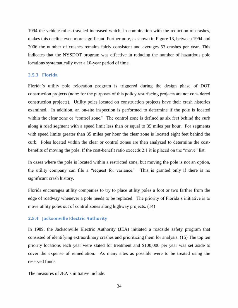
The “bad actor” list published in 1984 identified 567 sites. In 1994, 262 sites were identified, a
reduction of 54 percent in ten years. (15)
Moreover, there were only 57 crashes resulting in 64 fatalities in 1994, when compared with the
more than 100 fatalities in 1982 when the remediation program began, there is a clear decline in
crashes as well as fatalities. While this value may not seem considerable, between 1982 and
Figure 13 - Number of Utility Pole Crashes in New York State from 1994-2006 (3)
0102030405060708090
100
19
94
19
95
19
96
19
97
19
98
19
99
20
00
20
01
20
02
20
03
20
04
20
05
20
06
Nu
mb
er
of
Cra
she
s
Year
Figure 12 - After Pole Relocation (23)
Figure 11 - Before Pole Relocation (23)
34
1994 the vehicle miles traveled increased which, in combination with the reduction of crashes,
makes this decline even more significant. Furthermore, as shown in Figure 13, between 1994 and
2006 the number of crashes remains fairly consistent and averages 53 crashes per year. This
indicates that the NYSDOT program was effective in reducing the number of hazardous pole
locations systematically over a 10-year period of time.
2.5.3 Florida
Florida‟s utility pole relocation program is triggered during the design phase of DOT
construction projects (note: for the purposes of this policy resurfacing projects are not considered
construction projects). Utility poles located on construction projects have their crash histories
examined. In addition, an on-site inspection is performed to determine if the pole is located
within the clear zone or “control zone.” The control zone is defined as six feet behind the curb
along a road segment with a speed limit less than or equal to 35 miles per hour. For segments
with speed limits greater than 35 miles per hour the clear zone is located eight feet behind the
curb. Poles located within the clear or control zones are then analyzed to determine the cost-
benefits of moving the pole. If the cost-benefit ratio exceeds 2:1 it is placed on the “move” list.
In cases where the pole is located within a restricted zone, but moving the pole is not an option,
the utility company can file a “request for variance.” This is granted only if there is no
significant crash history.
Florida encourages utility companies to try to place utility poles a foot or two farther from the
edge of roadway whenever a pole needs to be replaced. The priority of Florida‟s initiative is to
move utility poles out of control zones along highway projects. (14)
2.5.4 Jacksonville Electric Authority
In 1989, the Jacksonville Electric Authority (JEA) initiated a roadside safety program that
consisted of identifying extraordinary crashes and prioritizing them for analysis. (15) The top ten
priority locations each year were slated for treatment and $100,000 per year was set aside to
cover the expense of remediation. As many sites as possible were to be treated using the
reserved funds.
The measures of JEA‟s initiative include:
35
New aboveground facilities are to be placed as far from the roadway as is practical.
The longest feasible span length between poles is used in order to reduce the number of
necessary utility poles.
Locations with significant previous accident experience are to be addressed with safety
measures.
Avoid the placement of poles in susceptible locations such as medians, traffic islands and
lane terminations. (15)
2.5.5 Georgia
Relocating all utility poles located in the clear zone on all U.S. and state roads in the subsequent
30 years is the goal of Georgia‟s Clear Roadside Program. (14) Georgia plans to meet this goal
by relocating 250 poles a year. In order to gain support for this initiative, Georgia relaxed its
rules on pole attachments. Existing poles that companies previously would have been denied
permission to attach to are now conditionally permissible; poles that qualify cannot have a
significant crash history.
Georgia identifies sites for remediation by checking three mile long segments of state-controlled
roads for total utility pole-related accidents over the previous three years to determine the “worst
offenders.” Poles and pole lines that do not meet the roadway requirements are subject to
relocation. Georgia‟s roadway requirements are the same as those set forth by Florida, the
minimum setback in zones where the speed limit exceeds 35 miles per hour is eight feet from the
curb and six feet for zone with speed limits less than 35 miles per hour. Ideally a 12 foot
minimum setback is desired in all curbed conditions. (14)
2.5.6 Pennsylvania
Unlike programs for utility pole remediation established in Georgia, Florida and New York,
Pennsylvania will not concentrate on highway construction projects, rather the plan calls for the
relocation of utility poles in “hit pole clusters.” “Hit pole clusters” are identified as half mile
segments of roadway with three crashes within a five year period. Relocation will not be
attempted, however, unless the pole(s) in question can be moved at least five feet. (14)
Among the initiatives put in place to reduce crashes at are:
Relocate poles at the expense of pole owners with the assistance of PennDOT.
Placement of rumble strips at the edge of the roadway to keep motorists on the road.
36
Placement of reflective tape around poles where relocation is not a viable alternative. (15)
An additional difference between Pennsylvania and other States is the way costs associated with
relocation of the poles are assessed. While most other policies require utility companies to cover
the costs of relocation, Pennsylvania‟s program anticipates the equal distribution of costs
between the DOT and the utility in certain cases. The division of the cost is dependent on the
situation. If the utilities are being moved underground or out of an existing right of way (ROW),
the DOT will be responsible for 50 percent of costs. In cases where the pole is moved within the
ROW, the utility company is entirely responsible for the costs. (14)
2.5.7 Washington State
Washington State Department of Transportation (WSDOT) developed a program for clearing the
roadside of utilities at the prompting of the Federal Highway Administration (FHWA) in 1986.
The policy consists of locating new utilities outside of the clear zone, moving or mitigating
objects during highway construction projects and systematically remediating existing utility
objects to meet the annual mitigation target.
The WSDOT in conjunction with utility companies has created a plan to systematically reduce
the risk of collision with utility objects. WSDOT and the utility companies work together to
classify utility objects that are located in the control zone into three classes: Location I, Location
II and Location III.
Location I objects are located:
On the outside of horizontal curves where the speed limit on the curve is 15 miles per
hour or more below the speed posted on that segment of highway,
Where a roadside feature is likely to direct the vehicle into the utility object,
Less than five feet from the edge of the shoulder, or
Within the turn radius area of public grade intersections.
Approximately 20 percent of utility objects are categorized as Location I objects. Location II
objects are those not classified as Location I or Location III and constitute 32 percent of utility
objects in the state of Washington. The remaining 48 percent are deemed Location III objects.
Location III objects are defined as objects located:

37
Outside of the control zone,
Inside of the control zone but have mitigated impact risks with safety measures such as
frangible poles, or
Located in a protected or inaccessible area.
It is the goal of the policy to make all utility objects Location III over time wherever possible and
practical. Location I objects are to be moved to Location III or mitigated. If analysis determines
this is not possible, then a variance can be submitted. Location II objects must undergo
engineering analysis in addition to AASHTO‟s cost-effective procedure to determine the best
course of action, whether it is relocation, mitigation or reclassification.
Initially, remediation of existing utility objects (that were not located on highways which were
anticipated to undergo construction) was triggered by the renewal of the franchise agreement
between the state and utility company. Companies were required to relocate or mitigate utilities
within one year of renewal. However, this policy created concern that the expense of
remediation would be excessive for such a short period of time. Instead, an annual mitigation
target (AMT) was created in place of the franchise trigger. The AMT is based on the number of
utilities in need of remediation, as well as the size and available resources of the utility company.
The AMT is calculated using the following relationship:
Where:
M = number of miles of utility owned aboveground facilities located within the highway
right of way (miles)
N = utility‟s average line span length (feet)
Z = percent of objects owned by the utility that are estimated to be in Location I or II
Y = number of years for compliance (50 years maximum)
If the company fails to meet its AMT in a given year, the required number of objects that must be
remedied the following year will be increased accordingly. Companies that exceed the required
Equation 8

38
Figure 14 - TTI Model of a Ground Level Slip Base &
Upper Hinge Assembly Prototype Breakaway Utility Pole
AMT in one year may reduce the number in the following year. Objects that must be mitigated
or relocated as a result of a highway construction project can be counted toward AMT. As of
2001, WSDOT has experienced a 35 percent decrease in pole related accidents. (15)
2.5.8 Lafayette Utilities System
According to Ivey and Scott, the Lafayette Utilities System (LUS) has put into practice a
procedure for reducing the number of accidents involving utility structures and improving public
safety. The simplified approach implemented by LUS consists of the following steps:
1. Examine collisions with utility objects to discern if sites are predisposed to recurring
collisions or only suffer from a random collision.
2. Perform predictive analysis along busy roads to calculate the relative likelihood of
collisions at specific sites or areas.
3. Determine the relative conformity with the RDG of priority sites identified in step 2.
4. Apply safety treatments to the top ten sites each year.
When LUS is no longer able to identify sites where safety improvements would result from
remediation, the primary goals of the program will be met. (15)
2.6 Steel Reinforced Safety Poles
In the 1980‟s the FHWA supported research to
develop a cost-effective “yielding” timber
utility pole that would improve the security of
passengers in a vehicle impacting a utility pole.
Scott and Ivey estimate that Steel Reinforced
Safety Poles (SRSP) reduce the likelihood of
injury in a high-speed collision from 77 percent
to less than one half of one percent. (16),(15)
The Hawkins Breakaway System (HBS) was
the resultant design. (17) After successful crash
testing was performed at the Texas
Transportation Institute (TTI), HBS was
cleared for selective implementation. Figure
14 displays a model of a prototype breakaway
39
utility design.
Field tests were performed in Boston, Massachusetts and the HBS design was considerably
modified for installation. The modified design was termed the FHWA or Massachusetts design.
The modified devices were also installed in Kentucky. The installations were evaluated over a
two year period and no serious problems were encountered. In both states, the poles were found
to perform well under high wind speeds, and in Massachusetts the poles did not fail as a result of
exposure to ice or snow. While the poles in Kentucky did not experience any collisions, there
were five crashes involving the Massachusetts poles. There were no serious injuries; no loss of
utility service and the necessary repair time was approximately 90 minutes. In 1992, a thorough
report was prepared to evaluate and record the in-field performance of the Massachusetts poles.
After the assessment the poles were elevated from experimental to operational status. At present,
some of the poles are still in service and are in good condition. (16)
The Massachusetts design was modified and renamed AD-IV. In 1994, AD-IV poles were
installed in Texas, and over the three year evaluation period sustained no damage as a result of
high winds or hail. The only collision that has happened with any of the AD-IV poles took place
with an improperly installed device, however, the pole still performed adequately and no serious
injuries occurred. Unfortunately, the entire pole had to be replaced after the impact. In 1995,
FHWA poles were installed in Virginia and evaluated. (18) During this study there were no
maintenance costs or issues, no damage resulted from high winds, but no collisions occurred to
allow the evaluation of the impact behavior. The steel reinforced safety poles were found to
perform well and in Massachusetts the poles were determined to be economical. (15)
The installation cost of the Massachusetts design was about $5,600 total cost per pole (which
included $2,600 in materials and $3,000 in labor and equipment) at the time of the evaluation in
1992. (18) This is more than the cost of a traditional timber utility pole installation, which costs
approximately $3,250 (based on a 2003 cost estimate which assumes a $3000 installation cost
and a materials cost of $250). (19) However, Pacific Institute for Research and Evaluation
(PIRE) currently estimates the societal cost of a fatal crash to be $3.841 million on average; this
value includes direct expenditures such as court expenses, police, paramedics and Medicaid in
addition to indirect costs such as lost wages, subsequent traffic jams, and a lower quality of life.

40
PIRE estimates injuries cost on average just $50,512; when compared with the costs associated
with a fatal crash the difference is evident. (20) Breakaway poles were deemed cost-effective
despite their increased installation expense because they have successfully reduced the severity
of crashes with utility poles. The five crashes during the Massachusetts in-field evaluation
resulted in zero fatalities and no serious injuries. In addition, the time and consequently cost of
fixing a breakaway pole after a collision is reduced because the top of the breakaway pole is
suspended with guy lines, making it no longer necessary to temporarily relocate service because
wires are prevented from breaking and disrupting service. (18)
2.7 Delineation
Delineation is another potential method of reducing the risk of a crash occurring, by placing
reflectors on utility poles motorists can be made aware of their presence and hopefully avoid
these objects. According to Ivey and Scott, in an effort to improve roadside safety when
relocation, removal and shielding are not viable options for mitigating risk, the FHWA and the
Maryland State Highway Administration have undertaken a study to find effective and efficient
methods of reducing risk associated with hazardous fixed objects. The study delineated all fixed
objects using yellow reflective material for demarcation. The effects of delineation have not
been statistically verified as yet. (15)

41
3 Methodology
Initially, the goal of this study was to perform an ISPE and develop a standard operating
procedure for the placement of new utility poles and relocation of existing poles; however due to
time constraints the scope and expected results of this study had to be reduced. The primary
objective of this project was to validate or develop a predictor model which could be used to
identify high risk utility poles based on the geometry of the road and the characteristics of the
pole site. The study first needed to identify a study area, and then collect data along this route.
Since previous studies had developed their own predictor models for identifying high risk
locations it was decided to first attempt to validate one of these models. Since Fox, Good and
Joubert‟s model required many characteristics that were not available for the study route, it was
decided that it would not be used for this study. Mak and Mason‟s model was also very
involved, moreover the research team had not verified that this model was applicable since data
from non-crash sites had not been applied. Ivey and Zegeer‟s model, on the other hand, is simple
and the necessary variables are available; therefore this study first attempted to validate this
model. In the event the model developed by Ivey and Zegeer cannot be validated, then a model
using the data collected by this study will be developed.
3.1 Identification of a Study Area
Before data collection could begin, a suitable study area had to be established. The process used
to identify the study area was modified from the method used by a similar study currently being
performed at WPI on tree crashes. The tree research team had initially attempted to determine a
study area by mapping crash locations using GPS coordinates provided in the state crash
database. The researchers were unable to recognize any areas that experienced significantly
more crashes than any other; however, they did identify a trend, and it appeared from their initial
mapping that crashes occurred more often on rural and local roads. As a result, they adjusted
their approach for determining a study area; instead they identified the roadway functional class
with the highest crash rate. Crash rates are a widely accepted way of comparing crash statistics
because they allow a person to evaluate crashes occurring on roads of varying lengths and
different Annual Average Daily Traffic (AADT). In order to calculate the crash rate of each
roadway functional class first they had to identify the roadway functional class of the roads with

42
crashes as well as the AADT of the crash locations. The following equation (Equation 9) was
used to calculate crash rate:
Their investigation determined that rural collectors experienced more crashes per 100 million
vehicle miles traveled (MVMT) than the other functional classes.
Because this method was successful at narrowing the study area, this study also identified the
study area using crash rates by roadway functional class. But the technique was modified to
minimize the need for data farming. Rather than determining the length and AADT of each
functional class of road in Massachusetts, the vehicle-miles of travel by functional system was
taken from Highway Statistics available on the U.S. Department of Transportation Federal
Highway Administration website. The number of crashes on each functional class was retrieved
from the Fatality Analysis Reporting System (FARS) encyclopedia. (3)
Table 6, shown below lists the number of vehicle miles traveled (in millions) by roadway
functional class, as well as the fatal crashes, total crashes and crash rates.
Equation 9

43
Table 6 - Crash Rates by Roadway Functional Class Y
ea
r
Roadway Function
Class
URBAN
Interstate Other
Principal Arterial
Minor Arterial
Major Collector
Minor Collector
Local Total
20
03 Vehicle Miles Traveled (in millions) 14,471 4,985 11,526 8,483 2,849 7,193 49,507
Fatal Crashes 0 7 19 5 2 33
Total Crashes 0 9 23 8 6 46
20
04 Vehicle Miles Traveled (in millions) 15,273 5,143 11,421 8,647 2,860 7,282 50,626
Fatal Crashes 3 4 16 7 2 32
Total Crashes 5 5 20 12 4 46
20
05 Vehicle Miles Traveled (in millions) 15,306 5,732 11,199 8,712 2,974 7,296 51,219
Fatal Crashes 8 0 13 6 5 32
Total Crashes 9 0 17 8 7 41
3 y
ears
MVMT 45,050 15,860 34,146 25,842 8,683 21,771 151,352
Fatal Crashes 11 11 48 18 0 9 97
Total Crashes 5 14 43 20 0 10 92
Fatal Rate 0.0244 0.0694 0.1406 0.0697 - 0.0413 0.0641
Total Rate 0.0111 0.0883 0.1259 0.0774 - 0.0459 0.0608
Ye
ar
Roadway Function
Class
RURAL
Interstate Other
Principal Arterial
Minor Arterial
Major Collector
Minor Collector
Local Total
20
03 Vehicle Miles Traveled (in millions) 1,258 812 638 658 155 681 4,202
Fatal Crashes 0 0 1 3 0 3 7
Total Crashes 0 0 1 5 0 4 10
20
04 Vehicle Miles Traveled (in millions) 1,294 794 593 622 156 686 4,145
Fatal Crashes 0 3 3 4 2 1 13
Total Crashes 0 3 3 6 3 3 18
20
05 Vehicle Miles Traveled (in millions) 1,285 835 650 627 155 687 4,239
Fatal Crashes 0 0 1 1 2 0 4
Total Crashes 0 0 1 2 2 0 5
3 y
ea
rs
MVMT 3,837 2,441 1,881 1,907 466 2,054 12,586
Fatal Crashes 0 3 5 8 4 4 24
Total Crashes 0 3 4 11 3 7 28
Fatal Rate - 0.1229 0.2658 0.4195 0.8584 0.1947 0.1907
Total Rate - 0.1229 0.2127 0.5768 0.6438 0.3408 0.2225
Based on the analysis above, rural minor collectors have the highest fatal and total crash rate
(highlighted in yellow) followed by rural major collectors (highlighted in orange). Since rural

44
collectors are the most dangerous roadway functional class, a rural collector in close proximity to
WPI with a history of utility pole crashes was chosen for further investigation. Route 31 in
Spencer, MA alternates between a minor and major collector and is within 30 minutes of driving,
making it a good candidate for more in-depth study.
3.2 Data collection
Once the study area was identified, necessary roadway characteristics and a method of data
collection had to be determined. In addition, it is important that data is collected for both poles
that have already been hit and those that have not. In order to identify crash sites, a
comprehensive database of statewide crashes furnished by MassHighway was sorted based on
most harmful event. Only collisions involving utility poles as the most harmful event were
considered, all crashes involving other fixed objects were discarded. The evaluation was
performed using three years of data obtained from the years 2003, 2004 and 2005. With the
locations of previous crash sites in hand, attention turned to deciding upon necessary data fields
and developing a method of collecting the data. Existing models found in the literature review
were referred to for inspiration. It was determined that it would be necessary to collect:
Roadway geometry such as horizontal curvature and grade,
Lateral offset,
Speed limit,
Location of pole relative to horizontal alignment (inside or outside of curve or at point of
tangency),
Location of pole relative to the vertical alignment (at the top, middle, or bottom of the
hill),
Density of utility poles,
Intersection type (signalized or unsignalized),
Proximity to other fixed objects (mainly guardrail),
Pavement deficiencies (i.e. rutting, potholes, cracking, frost heaves),
Width of road, and
Annual average daily traffic.
Most of the data could only be collected in the field; however, wherever possible the information
was farmed in the office from existing data or available resources. All information was stored in

45
Microsoft Excel workbooks in order to facilitate later analysis. Refer to Appendix B – Data
Collection Sheets on page 71 to view the data collected.
3.2.1 Stations
An organized method of identifying data points had to be utilized to allow cross-referencing and
the ability to return to the same site if necessary to collect more data, especially since the route
was approximately 9.8 miles long. It was decided the best method of doing this would be to use
a baseline with stations going south to north along Route 31. Initially, stations were measured by
driving a 1997 SAAB Turbo along the edge of the road heading north and using the odometer to
measure 0.1 mile increments. After approximately three miles the nature of the road changed the
unpaved shoulders decreased in size and eventually were eliminated and the traffic increased, as
well making it unsafe to continue making frequent stops in a vehicle. A new method of
measuring stations had to be devised that would be safe and accurate. So a surveyor‟s wheel
which works well on pavement (see Figure 15 and Figure 16) was used to measure the remainder
of the route.
Figure 16 –Hodometer’s measuring device
Figure 15 – Surveyor’s Wheel a.k.a. Hodometer

46
3.2.2 Lateral Offset
Lateral offset was measured using two methods: a Sonin® Multi-Measure® Combo Pro
Electronic Distance Measuring tool shown in Figure 17 (on page 46) as well as a Lufkin Tufboy
100 foot decimal surveyor‟s tape measure featured in Figure 18. The measurements were taken
from the edge of the traveled way to the front of the utility pole. The edge of the traveled way
was defined as the edge of the single white line (SWL) where it existed; if there was no SWL the
front of the curb and/or the edge of the pavement (EOP) marked the edge of the traveled way. If
the utility pole was located behind a guardrail, the measurement was taken from the edge of the
traveled way to the front of the guardrail (FOG), and another measurement was taken from the
FOG to the front of the utility pole. Measurements were always taken perpendicular to the edge
of the road so the minimum lateral offset was recorded.
3.2.3 Density
Initially the utility pole density was calculated by assuming the average distance between poles
was equal to the measured distance between the first pole at a station and the second pole.
However this method was time consuming, inefficient and inaccurate. Since the Ivey & Zegeer
model required the number of poles in their model it made more sense to simply count and
Figure 18 – Surveyor’s Tape Measure
Figure 17 – Electronic Distance Measuring Tool
47
record the number of poles between stations, then average distance between the poles was
calculated from this.
3.2.4 Annual Average Daily Traffic
The Annual Average Daily Traffic (AADT) data was retrieved from the Central Massachusetts
Regional Planning Agency and the MassHighway website.
3.2.5 Horizontal and Vertical Alignment
The state of Massachusetts owns an Automatic Road Analyzer (ARAN), however it was not
equipped with all of the instrumentation and software necessary to complete all the data
collection with it. (21) Since this study did not have the budget to purchase the necessary
equipment or hire Fugro-Roadware or another company providing similar services, an alternative
economical method had to be developed. Due to equipment and time constraints surveying the
length of road was not a feasible option. The only other alternative was to use existing data.
Aerial photographs with spatial references are available on the MassGIS homepage, which were
downloaded and imported into Autodesk Civil3D. Once the images were opened in Civil3D, by
tracing the center line of the road and creating best fit curves, a horizontal alignment could be
created. See Figure 19, to view a portion of the horizontal alignment. Once the horizontal
alignment was created the x and y coordinates were available, but to get the grade of the road it
was still necessary to get the z coordinates. The surface of the area was created and exported
from Google Earth, these coordinates were then imported into Civil3D. By overlaying the
horizontal alignment on the surface, it was possible to extrapolate the corresponding z
coordinates. With the z coordinates a profile was created and under the assumption the road
roughly followed the shape of the surface elevation, a smooth curve was placed along the profile.
A portion of the vertical alignment is shown below in Figure 20.

48
Alignment data was tabulated and exported to Microsoft Excel. This produced two spreadsheets,
the first with the horizontal curves and the other with grade and these values were all given in
reference to the stations along the road. From Excel, the necessary data was extracted for each
station. See Appendix B – Data Collection Sheets for the complete tables.
3.2.6 Remaining Fields
Data fields such as speed limit, pavement deficiencies, placement of the pole relative to the
horizontal alignment (e.g., inside, outside or tangent to the curvature) and vertical alignment
(e.g., top, bottom or middle of a hill), pole number, and intersection type were all collected from
field observations.
Figure 20 – A portion of the vertical alignment
Figure 19 – A portion of the horizontal alignment and the aerial phtographs

49
3.3 Develop a Model using Collected Data
Using multiple regression analysis in Matlab, the least-squares fit model of the data, Equation
10, was created to estimate the crashes per mile per year using the site characteristics.
Equation 10
Where
For the model the average values of lateral offset, AADT, speed limit, grade, and horizontal
curvature were used as variables, as well as the sum of the utility poles per mile. In addition to
using the average value for the grade, it was assumed to be absolute since the sign of the slope
depended on the direction of vehicle travel. Since vehicles travel in both directions and crashes
could occur either way, it was decided to consider only how steep the grade was and not its
direction. To view the data used refer to Appendix E – Summary of Characteristics of 1 mile
Crash Segments.
Many of the variables behaved as anticipated based on the actual trends, for instance as the
horizontal curvature increases the estimated crashes per mile per year decreases (see Figure 24),
as the grade increases so does the estimate (see Figure 23), and the increase in speed results in a
decrease in reaction time and subsequently more crashes per mile per year (see Figure 25).
The increase in lateral offset should result in fewer crashes, this is the case with the actual data,
see Figure 21. Also the number of crashes is expected to increase as the number of utility poles
increases, just as it does according to the actual data displayed in Figure 22.
It was unexpected that predicted crashes would decrease with the increase in AADT. Logically,
as the number of vehicles on the road increases crashes would increase too, but the model may
not support this because of the limited amount of crash data available.

50
Figure 25- Crashes per mile per year versus Posted
Speed Limit
0
0.5
1
1.5
2
2.5
0 20 40 60Cra
she
s p
er
mile
pe
r ye
ar
Posted Speed Limit (mph)
Figure 24- Crashes per mile per year versus
Horizontal Curvature
0
0.5
1
1.5
2
2.5
0 500 1000Cra
she
s p
er
mile
pe
r ye
ar
Average Horizontal Curvature (feet)
Figure 23- Crashes per mile per year versus Grade
0
0.5
1
1.5
2
2.5
0.0000 0.0100 0.0200 0.0300 0.0400Cra
she
s p
er
mile
pe
r ye
ar
Average Grade
Figure 22- Crashes per mile per year versus Number
of Poles per Mile
0
0.5
1
1.5
2
2.5
0 20 40 60Cra
she
s p
er
mile
pe
r ye
ar
Number of Poles per Mile
Figure 21- Crashes per mile per year versus Lateral
Offset
0
0.5
1
1.5
2
2.5
0.00 5.00 10.00 15.00 20.00Cra
she
s p
er
mile
pe
r ye
ar
Lateral Offset (feet)

51
4 Analysis
4.1 Compare Ivey & Zegeer’s Predictions with Actual Data
In order to validate a model, it must be compared with a benchmark. The values calculated using
Ivey and Zegeer‟s predictor model were compared directly to the actual accidents per mile per
year (using data from 2003 to 2005). When accidents per mile per year were compared in this
manner the correlation was poor. This is not completely unexpected because Ivey and Zegeer
strongly suggest that their model be used solely for prioritization purposes not predicting the
expected number of accidents, so rather than attempting to directly compare accidents per mile
per year, the mile segments were prioritized using both the actual crash data (Table 6) and the
model (Table 7).
When compared in this manner, both the crash statistics and the model recognized that the mile
five segment (in red) is the area of highest concern. Although beyond that the model and actual
data differ somewhat. The discrepancy could possibly be due to the assumption that the average
lateral offset calculated using the lateral offset from each station would be representative of the
actual average lateral offset of the mile segment. To determine if this is the source of the
incongruity the lateral offset data is recollected, this time for all utility poles along Route 31 in
Spencer.
Table 8 – Ivey & Zegeer’s Predicted Priorities
Mile Accidents/mi/yr
5 2.7045
6 1.4607
7 1.0957
4 0.9931
8 0.9564
9.8 0.9536
3 0.9195
1 0.8174
9 0.8111
2 0.8003
Stations - Ivey & Zegger
Table 7 – Actual Crash Data Priorities
Mile Accidents/mi/yr
5 2
7 1.3333
3 1
9 1
2 0.3333
8 0.3333
1 0
4 0
6 0
9.8 0
Actual

52
4.2 Recollect Lateral Offset & Density Data
After comparing the actual crash data to the prioritized locations identified by Ivey & Zegeer‟s
model it was deemed necessary to return to the field to collect lateral offset data on all utility
poles along the route in order to get a more accurate prioritized list and hopefully better
correlation between the actual crashes and predicted crashes. (See Appendix C – Average Lateral
Offset Data Collection Sheets on page 82 for the additional lateral offset data.) In addition to
getting the true average lateral offset, rather than an estimated average lateral offset, the density
was adjusted. Initially every pole was counted and since measurements were only taken at
stations, poles located behind guardrail were included in the density. With the more complete
lateral offset data it was possible to identify all the poles that were located behind guardrail.
However, the poles behind the guardrail could not simply be dismissed because several of the
utility poles were located less than three feet behind the guardrail and in some cases right behind
it (refer to Figure 26 on page 53), which does not allow the guardrail to properly deflect and the
vehicle would still come in contact with the utility pole. In addition, some poles were located
behind the guardrail but the guardrail was not at the height necessary to deflect a vehicle (see
Figure 27). The density was adjusted to include poles that were not behind guardrail and poles
that were less than three feet from the front of the guardrail or if the guardrail was an insufficient
height to prevent the vehicle from reaching the pole. Poles that were more than 30 feet from the
edge of the traveled way and poles that were more than three feet behind the guardrail were not
included in the density because the guardrail has sufficient room to deflect and redirect the
vehicle.

53
4.3 Recalculate Ivey and Zegeer’s Model & Compare to Actual Crash Data
Using the adjusted values for average lateral offset and density (see Appendix C – Average
Lateral Offset Data Collection Sheets), the accidents/mile/year were recalculated using Equation
7. These values were prioritized and compared with the actual crash data as well as the original
calculations of Ivey & Zegeer‟s model; the priorities are shown below in Table 8 on page 54.
Figure 27 – Guardrail ends before pole
Figure 26 - Pole located right behind guardrail
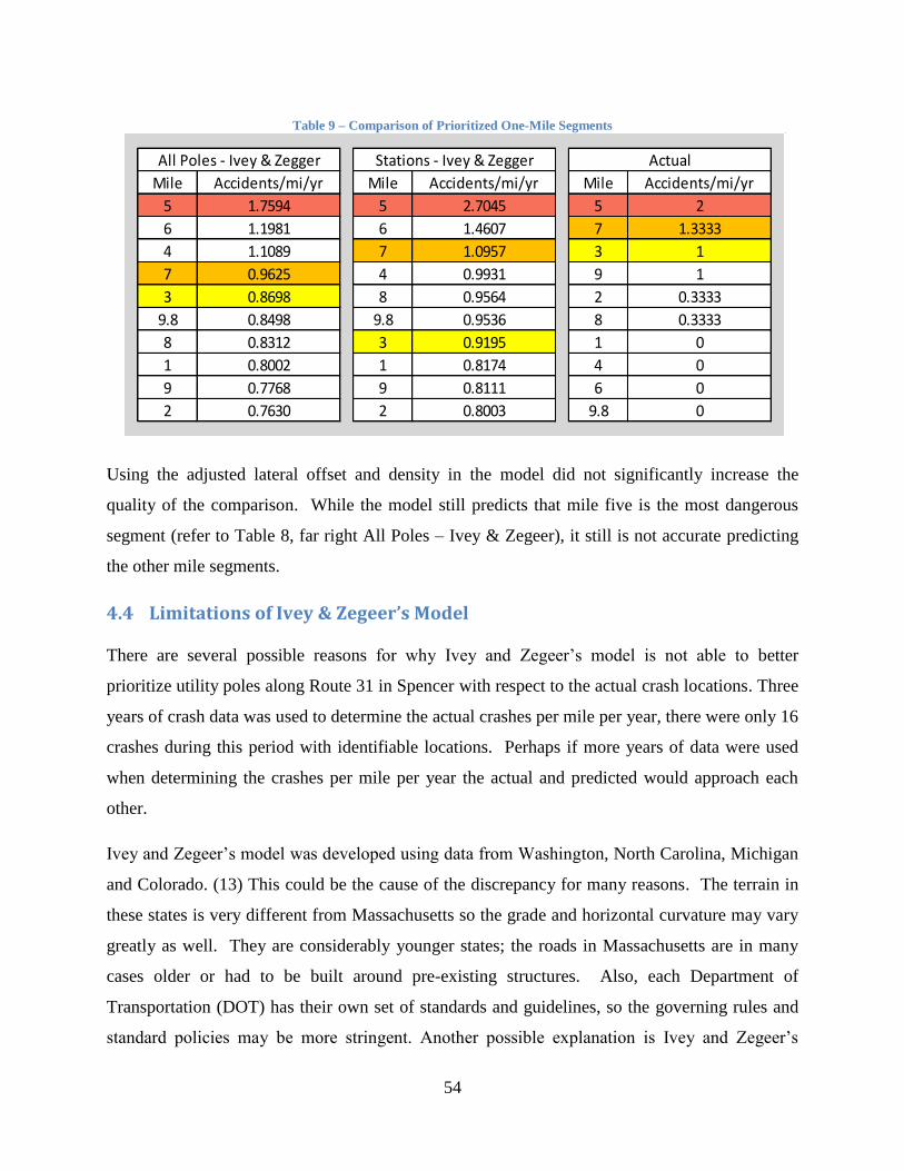
54
Using the adjusted lateral offset and density in the model did not significantly increase the
quality of the comparison. While the model still predicts that mile five is the most dangerous
segment (refer to Table 8, far right All Poles – Ivey & Zegeer), it still is not accurate predicting
the other mile segments.
4.4 Limitations of Ivey & Zegeer’s Model
There are several possible reasons for why Ivey and Zegeer‟s model is not able to better
prioritize utility poles along Route 31 in Spencer with respect to the actual crash locations. Three
years of crash data was used to determine the actual crashes per mile per year, there were only 16
crashes during this period with identifiable locations. Perhaps if more years of data were used
when determining the crashes per mile per year the actual and predicted would approach each
other.
Ivey and Zegeer‟s model was developed using data from Washington, North Carolina, Michigan
and Colorado. (13) This could be the cause of the discrepancy for many reasons. The terrain in
these states is very different from Massachusetts so the grade and horizontal curvature may vary
greatly as well. They are considerably younger states; the roads in Massachusetts are in many
cases older or had to be built around pre-existing structures. Also, each Department of
Transportation (DOT) has their own set of standards and guidelines, so the governing rules and
standard policies may be more stringent. Another possible explanation is Ivey and Zegeer‟s
Table 9 – Comparison of Prioritized One-Mile Segments
Mile Accidents/mi/yr Mile Accidents/mi/yr Mile Accidents/mi/yr
5 1.7594 5 2.7045 5 2
6 1.1981 6 1.4607 7 1.3333
4 1.1089 7 1.0957 3 1
7 0.9625 4 0.9931 9 1
3 0.8698 8 0.9564 2 0.3333
9.8 0.8498 9.8 0.9536 8 0.3333
8 0.8312 3 0.9195 1 0
1 0.8002 1 0.8174 4 0
9 0.7768 9 0.8111 6 0
2 0.7630 2 0.8003 9.8 0
All Poles - Ivey & Zegger Stations - Ivey & Zegger Actual

55
model, which prioritizes one mile segments, may be too long a segment for a road such as this
where the roadway geometry and characteristics vary in smaller segments. Along the same lines,
mile one was assumed to begin at the Charlton-Spencer town line and stations for the next mile
were assumed be a part of this mile. Perhaps segments should have been divided based on where
their characteristics changed rather than where they happened to begin relative to the town line.
In order to gain a better understanding of why Ivey and Zegeer‟s model does not correlate to the
actual site data, a spreadsheet was created that looked at common characteristics of stations with
a history of crashes. Shown below in Table 9 is a summary of the characteristics of each of the
16 crashes that occurred along the 9.8 mile stretch of Route 31 in Spencer.

56
Originally, there appeared to be a trend that as the number of poles increased so did the number
of crashes (refer to Appendix D – Characteristics of 0.1 Mile Crash Segments on page 93 to view
the complete table of site characteristics). But when the poles that were more than three feet
Table 10 - Common Characteristics of Stations with Crash History
# of Poles 1 2 3 4 5 6 7
# of Crashes 2 2 3 3 3 3 0
Offset (ft) 0-2.5 2.5-5 5-7.5 7.5-10 >10
# of Crashes 6 1 1 1 8
AADT 4600 7000
# of Crashes 5 11
Radius (m) 175 400 750 0-∞
# of Crashes 2 1 1 12
Placement I O Tan
# of Crashes 1 11 4
Grade % 0-2% 2-4% 4-6% >6%
# of Crashes 9 4 1 2
Vertical Alignment Top Bottom Middle Flat
# of Crashes 0 1 13 2
Speed (MPH) 25 30 40 45
# of Crashes 4 2 7 3
Type N/A U S
# of Crashes 13 2 1
Adjusted Density (# of Poles / 0.1 mile)
Vertical Alignment (grade %)
Relative Placement on Hill (Vertical Alignment)
Speed Limit (MPH)
Intersection Signalized/ Unsignalized
Lateral Offset (feet)
AADT
Horizontal Curvature
Inside or Outside of Horizontal Curve

57
behind a horizontal barrier or greater than 30 feet from the traveled way were not included in the
density, the distribution of crashes became evenly spread amongst the densities. While logically,
increasing the number of poles along the road would increase the risk of a motorist colliding with
a pole in a run off the road crash, the data collected does not support this assertion.
It was expected that the lower the lateral offset, the higher the risk of the utility pole being hit,
however there is a split in the data, just as many crashes occurred with utility poles which were
greater than ten feet from the edge of the traveled way as crashes with poles that were less than
2.5 feet from the edge of the road.
The only variable which performed as anticipated was the AADT, more than twice as many
crashes occurred on the portion of the route with a higher volume of traffic.
Since the increased density and decreased clear zone should have an impact on the risk, there
must be other factors counteracting or interacting with these variables resulting in the
discrepancy between expected and actual. It appears that the placement with respect to the
horizontal curve is also a contributory factor. In the majority of segments with crashes, the poles
were located on the outside of the curve. Also most crashes occurred on hills, the majority of
them in the middle of the alignment, although the grade was generally between zero and two
percent and nearly always less than four percent. Another important variable to note: segments
with lateral offset greater than 7.5 feet are in areas where the posted speed limit is 40 mph or
greater. The increased velocity of the vehicle decreases the amount of time the motorist has to
react in the event of a run off the road crash.
When the characteristics of mile segments were compiled (see Appendix E – Summary of
Characteristics of 1 mile Crash Segments) and checked for trends it was found that the segments
with the higher priority than the actual data predicted were straighter and had a lower gradient,
lower speed limit and in many cases curbs which may contribute to the lower than predicted
occurrence of crashes.
As previously mentioned, one of the possible reasons for the inconsistency between the model
predictions and the actual crash data is the manner in which the road is segmented. The road is
divided into one mile sections beginning from the Charlton-Spencer town line and going North
along Route 31. Rather than segmenting the road arbitrarily every mile, instead the road is

58
divided into sections where they significantly change characteristics. For instance the lateral
offset drastically decreases or the grade sharply increases or any combination of these. By
dividing the road using its characteristics ten segments were created. The tables in Appendix F –
Summary of Data for Segments determined by Road Characteristics were referred to for
identifying common characteristics; in addition, photos taken of the road at each station during
data collection were referred to for further insight into the road‟s characteristics.
Segment one, which is 1.2 miles and begins at Station 00+00 (shown below in Figure 28 ), was
found to be mostly straight-aways with gentle, sweeping curves that have a radius of curvature
exceeding 1475 feet. The grade is less than three percent at every station except the Station
00+00 where it equals approximately 4.39 percent. The average grade for this segment is 2.4
percent. The lateral offset averaged 7.32 feet from the edge of the pavement and there were on
average four poles per 0.1 mile. During the three year period, there were zero crashes on this
segment.
The next segment begins at Station 63+36, featured in Figure 29, and continues for 2.4 miles
until Station 184+80. The road here becomes steeper; the average grade is 2.9 percent. The poles
are located along the outside of the curves. The shoulder is unpaved and the dirt is washed out.
The edge of the pavement is jagged, the pavement itself is cracked and rutted, and there is no
white line marking the edge of the traveled way. While the average lateral offset is 6.71 feet, the
geometry and condition of the road make this segment more dangerous than the previous section,
consequently three crashes occurred on this segment.
Figure 29 - Station 63+36 North View
Figure 28 - Station 00+00 North View

59
At Station 184+80 the road again changes characteristics, see Figure 30, the density of homes
increases, the average lateral offset decreases to two feet and average number of poles per 0.1
miles increases to over five. The radius of curvature decreases, averaging 715 feet, but drops as
low as 575 feet in places. In addition to the tighter curves, the road becomes steeper, with the
gradient at some points exceeding eight percent and averaging 4.9 percent for the 1.5 mile
stretch. The road is curbed and there is no shoulder. The speed limit is reduced from 40 miles
per hour to 25 miles per hour to compensate for the decreased clear zones and more dangerous
geometry. Also during this segment the AADT increase from 4600 to 7000. Within this segment
(segment three), six crashes occurred between 2003 and 2005.
The road is in a relatively unpopulated area in segment four, which begins after Station 264+00
(shown below in Figure 31) and continues for 1.1 miles. There are few homes and the road has
an approximately one foot wide paved shoulder with wide clear zones or guardrail. The average
lateral offset to the object (utility pole or horizontal barrier in cases where the pole is less than
three feet from the guardrail) is 5.72 feet. The density of utility poles decreased from more than
five to about 4.5 poles per 0.1 mile. The average grade in the section also decreases to
approximately 2.2 percent. The horizontal radius of curvature is a minimum of 800 feet on non
tangent sections. Due to changes in the roadway geometry the speed limit through this area
returns to 40 miles per hour. In the three year period between 2003 and 2005 there was only one
crash on this segment.
The 0.9 mile section of road beginning at Station 322+08 (refer to Figure 32) is characterized by
tangent sections, an average lateral offset of 11.43 feet, and an average grade of 1.7 percent.
Figure 31 - Station 264+00 North View
Figure 30 - Station 184+80 North View

60
Oddly, there are three crashes along this section between 2003 and 2005; most likely due to the
high density of utility poles lining this portion of the route, several of the 0.1 mile stations in this
segment have seven utility poles. The next 0.9 mile segment, which starts at Station 369+60
(pictured below in Figure 33), averages 1.3 percent grade and its horizontal radius of curvature
exceeds 1300 feet. This section of road has an average lateral offset of approximately 12.0 feet
and an average density of four poles per 0.1 mile. Due to the decrease in density and large
increase lateral offset as expected the number of crashes on this segment is less than the previous
one, with only one crash during the three period.
The road yet again changes at Station 417+12, shown in Figure 34; the road remains relatively
straight and the average lateral offset increases to 12.77 feet. However, the grade becomes much
steeper varying between 2.15 percent and 7.89 percent and averages 4.5 percent. The speed limit
for the two-thirds of this segment is 45 miles per hour. During a three year period, on this 0.5
mile segment of road, two crashes occurred.
Beginning at Station 448+80, depicted below in Figure 35, the average lateral offset of the
utility poles increases significantly, all but one pole is greater than 30 feet from the traveled way,
and therefore the poles are not even included in density calculations. The only pole that is less
than 30 feet from the road is 26.7 feet from the single white line marking the edge of the travel
lane. The road is straight and the grade is approximately 4.5 percent. Since there were no poles
to hit, there were no crashes on this 0.4 mile segment of road.
Figure 33 - Station 369+60 North View
Figure 32 - Station 322+08 North View
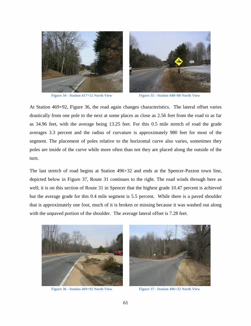
61
At Station 469+92, Figure 36, the road again changes characteristics. The lateral offset varies
drastically from one pole to the next at some places as close as 2.56 feet from the road to as far
as 34.96 feet, with the average being 13.25 feet. For this 0.5 mile stretch of road the grade
averages 3.3 percent and the radius of curvature is approximately 980 feet for most of the
segment. The placement of poles relative to the horizontal curve also varies, sometimes they
poles are inside of the curve while more often than not they are placed along the outside of the
turn.
The last stretch of road begins at Station 496+32 and ends at the Spencer-Paxton town line,
depicted below in Figure 37, Route 31 continues to the right. The road winds through here as
well; it is on this section of Route 31 in Spencer that the highest grade 10.47 percent is achieved
but the average grade for this 0.4 mile segment is 5.5 percent. While there is a paved shoulder
that is approximately one foot, much of it is broken or missing because it was washed out along
with the unpaved portion of the shoulder. The average lateral offset is 7.28 feet.
Figure 37 - Station 496+32 North View
Figure 36 - Station 469+92 North View
Figure 35 - Station 448+80 North View
Figure 34 - Station 417+12 North View
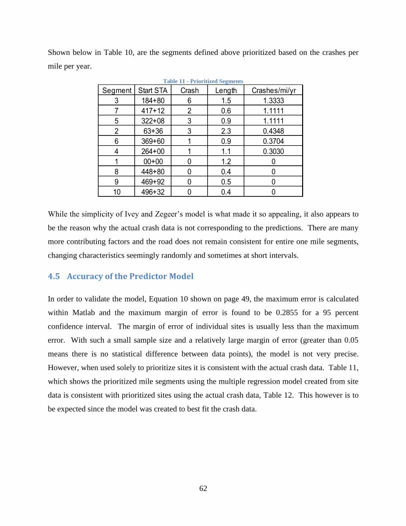
62
Shown below in Table 10, are the segments defined above prioritized based on the crashes per
mile per year.
While the simplicity of Ivey and Zegeer‟s model is what made it so appealing, it also appears to
be the reason why the actual crash data is not corresponding to the predictions. There are many
more contributing factors and the road does not remain consistent for entire one mile segments,
changing characteristics seemingly randomly and sometimes at short intervals.
4.5 Accuracy of the Predictor Model
In order to validate the model, Equation 10 shown on page 49, the maximum error is calculated
within Matlab and the maximum margin of error is found to be 0.2855 for a 95 percent
confidence interval. The margin of error of individual sites is usually less than the maximum
error. With such a small sample size and a relatively large margin of error (greater than 0.05
means there is no statistical difference between data points), the model is not very precise.
However, when used solely to prioritize sites it is consistent with the actual crash data. Table 11,
which shows the prioritized mile segments using the multiple regression model created from site
data is consistent with prioritized sites using the actual crash data, Table 12. This however is to
be expected since the model was created to best fit the crash data.
Table 11 - Prioritized Segments
Segment Start STA Crash Length Crashes/mi/yr
3 184+80 6 1.5 1.3333
7 417+12 2 0.6 1.1111
5 322+08 3 0.9 1.1111
2 63+36 3 2.3 0.4348
6 369+60 1 0.9 0.3704
4 264+00 1 1.1 0.3030
1 00+00 0 1.2 0
8 448+80 0 0.4 0
9 469+92 0 0.5 0
10 496+32 0 0.4 0

63
It is imperative that more data be collected; with a larger sample size and more data to analyze a
statistically significant model can be developed and then verified for other locations.
Table 13 - Actual Crash Data Priorities
Mile Accidents/mi/yr
5 2
7 1.3333
3 1
9 1
2 0.3333
8 0.3333
1 0
4 0
6 0
9.8 0
Actual
Table 12 – Equation 9 Predicted Priorities
Mile Crashes/mi/yr
5 1.8995
7 1.1707
3 0.5745
9 0.5444
8 0.4363
2 0.4305
4 0.2997
6 -0.022
9.8 -0.025
1 -0.293
Multiple Regression Model
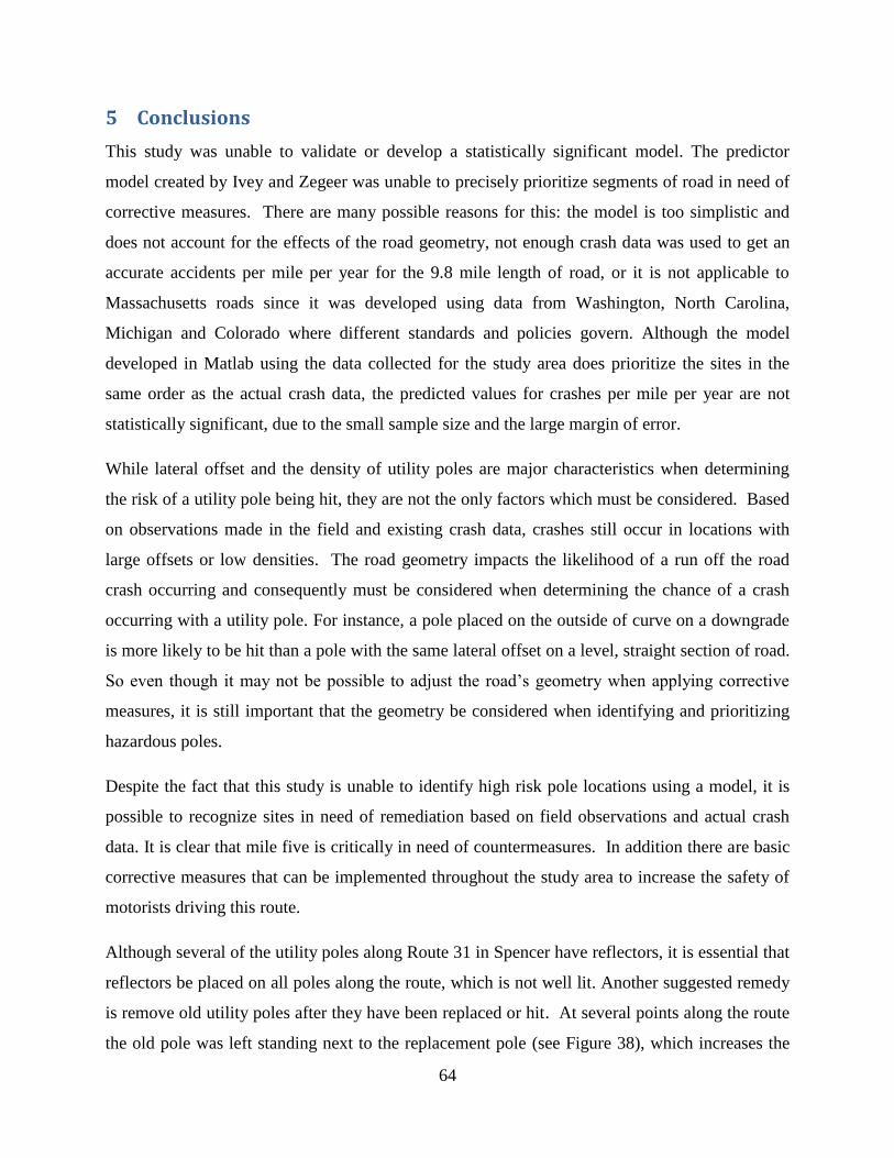
64
5 Conclusions
This study was unable to validate or develop a statistically significant model. The predictor
model created by Ivey and Zegeer was unable to precisely prioritize segments of road in need of
corrective measures. There are many possible reasons for this: the model is too simplistic and
does not account for the effects of the road geometry, not enough crash data was used to get an
accurate accidents per mile per year for the 9.8 mile length of road, or it is not applicable to
Massachusetts roads since it was developed using data from Washington, North Carolina,
Michigan and Colorado where different standards and policies govern. Although the model
developed in Matlab using the data collected for the study area does prioritize the sites in the
same order as the actual crash data, the predicted values for crashes per mile per year are not
statistically significant, due to the small sample size and the large margin of error.
While lateral offset and the density of utility poles are major characteristics when determining
the risk of a utility pole being hit, they are not the only factors which must be considered. Based
on observations made in the field and existing crash data, crashes still occur in locations with
large offsets or low densities. The road geometry impacts the likelihood of a run off the road
crash occurring and consequently must be considered when determining the chance of a crash
occurring with a utility pole. For instance, a pole placed on the outside of curve on a downgrade
is more likely to be hit than a pole with the same lateral offset on a level, straight section of road.
So even though it may not be possible to adjust the road‟s geometry when applying corrective
measures, it is still important that the geometry be considered when identifying and prioritizing
hazardous poles.
Despite the fact that this study is unable to identify high risk pole locations using a model, it is
possible to recognize sites in need of remediation based on field observations and actual crash
data. It is clear that mile five is critically in need of countermeasures. In addition there are basic
corrective measures that can be implemented throughout the study area to increase the safety of
motorists driving this route.
Although several of the utility poles along Route 31 in Spencer have reflectors, it is essential that
reflectors be placed on all poles along the route, which is not well lit. Another suggested remedy
is remove old utility poles after they have been replaced or hit. At several points along the route
the old pole was left standing next to the replacement pole (see Figure 38), which increases the

65
density of utility poles thereby increasing the risk of a crash occurring. Perhaps even more
disturbing is remnants of a hit utility pole were left alongside the road creating another object for
motorists to crash into, refer to Figure 39.
It is clear that a utility pole problem exists and it is important that research in this area continues
until a method of identifying at-risk poles and corridors is developed so hazardous poles can be
addressed before a crash occurs.
Figure 39 – Remains of Hit Pole Left alongside Road
Figure 38 - Two Poles Side by Side

66
6 Recommendations for Future Work
It was the initial goal of this project to complete an ISPE, create a method for identifying high
risk poles and develop a standard operating procedure. Due to time constraints much of this was
not completed. More extensive data collection is recommended in order to validate either Ivey
and Zegeer‟s model or the linear multiple regression model developed by this study. If neither of
these models is determined to be precise after more research it is suggested the data be used to
create a statistically significant model that is applicable to Massachusetts roads. The model
developed by this study treated the variables as independent; however there appears to be many
relationships between the variables and some dependency. A different form of equation may
better express these relationships and therefore the risk.
While general methods of remediation have been outlined, it is necessary to have site specific
information in order to perform cost-benefit analysis and make the best decision for the location.
Once a more precise model is developed, hazardous locations can be identified and methods of
remediation can be determined.
Finally, a standard operating procedure should be developed for the placement of new utility
poles as well as for the relocation of existing poles that are deemed dangerous.
67
Works Cited
1. Holdridge, Jason M., Shankar, Venky N. and Ulfarsson, Gudmundur F. The crash
severity impacts of fixed roadside objects . 2005.
2. Pfefer, R. and Slack, K. NCHRP Report 500 Volume 8: A Guide for Reducing Collisions
Involving Utility Poles. Washington D.C. : TRB, National Research Board, 2004.
3. Fatality Analysis Reporting System Encyclopedia. FARS Fatality Analysis Reporting System .
[Online] United States Department of Transportation, National Highway Traffic Safety
Administration, National Center for Statistics and Analysis, 1975. [Cited: April 13, 2008.]
http://www-fars.nhtsa.dot.gov/Main/index.aspx.
4. Safer roadsides through better utility pole placement, protection, construction. Ivey, D. and
Scott, P.
5. Ray, M.H., Weir, J. and Hopp, J. NCHRP Report 490: In Service Performance of Traffic
Barriers. Washington D.C. : TRB, National Research Board, 2003.
6. Ross Jr, H.E., Sicking, D.L. and Zimmer, R.A. National Cooperative Highway Research
Program Report 350: Recommended Procedures for the Safety Performance Evaluation of
Highway Features. Washington D.C. : Transportation Research Board, National Research
Council, 1993.
7. Officials, American Associates of State Highway and Transportation. Roadside Design
Guide. 3rd Edition. Washington D.C. : AASHTO, 2006. pp. 4-1 - 4-15.
8. Good, M.C. and Joubert, P.N. A review of roadside objects in relation to road safety. s.l. :
Austrailian Government Publishing Service, 1973. Report No. NR/12.
9. Wentworth, J.A. Motor vehicle accidents involving utility pole: summary of data availability.
s.l. : Offices of Research and Development, Federal Highway Administration, 1973.
10. Single-vehicle accident involving utility poles. Graf, N.L., Boos, J.V. and Wentworth, J.A.
1, s.l. : Public Roads, 1975, Vol. 39.
11. Fox, J.C., Good, M.C. and Joubert, P.N. Collisions with Utility Poles. 1979.
12. Mak, King K. and Mason Ph.D., Robert L. Accident Analysis - Breakaway and
NonBreakaway Poles Including Sign and Light Standards along Highways volume II - Technical
Report. 1980.
13. Ivey, D. and Zegeer, C. TRB State of the Art Report 9 Utilities and Roadside Safety:
Strategies. Washington, D.C. : National Research Council, 2004.

68
14. Lindly, Jay K. Dreft State Utility Pole Safety Program for Alabama. 2003.
15. Ivey, D. and Scott, P. TRB State of the Art Report 9 Utilities and Roadside Safety:
Initiatives. Washington, D.C. : National Research Council, 2004.
16. Ivey, Don L. and Scott, P. Safer roadsides through better utility pole placement, protection,
construction. Texas Transportation Institute. [Online] [Cited: April 14, 2008.]
http://tti.tamu.edu/publications/researcher/newsletter.htm?vol=35&issue=1&article=1.
17. Timber Pole Safety by Design. Ivey, D.L. and Morgan, J.R. Washington, D.C. :
Transportation Research Record.
18. Administration, Federal Highway. TE-24 Field Evaluation of Breakaway Timber Utility
Poles: Breaking Away to Save Lives. Highway Technet. [Online] [Cited: April 15, 2008.]
http://www.library.unt.edu/gpo/OTA/tech/safety/te24.html.
19. Western Wood Preservers Institute. Pressure Treated Wood Proves to be the Most Cost
Efficient Building Material. [Online] March 2003. [Cited: April 15, 2008.]
http://www.wwpinstitute.org/pdffiles/CAissues/MATERIALCOSTfinal.pdf.
20. AAA Newsroom. AAA. [Online] April 4, 2008. [Cited: April 15, 2008.]
http://www.aaanewsroom.net/Main/Default.asp?CategoryID=7&ArticleID=601.
21. Fugro-Roadware, around the world. Roadware GRP. [Online] [Cited: April 16, 2008.]
http://www.roadware.com/client_list/.
22. Labra, John J. and Michie, Jarvis D. The Utility Pole and Roadside Safety. 1986.
23. Administration, Office of Program. Utility Relocation and Accommodation on Federal-Aid
Highway Projects. s.l. : Federal HIghway Administration, 2003.
24. Mahoney, Kevin M, Julian, Frank and Taylor, Harry W., Jr. Good Practices:
Incorporating Safety into Resurfacing and Restoration Projects . s.l. : U.S. Department of
Transportation Federal Highway Administration , December 2006. FHWA-SA-07-001 .
25. [Online] [Cited: April 14, 2008.]
http://tti.tamu.edu/publications/researcher/v35n1/images/top.jpg.
26. [Online] [Cited: April 15, 2008.] http://blog.pennlive.com/lvbreakingnews/191crash.JPG.
27. [Online] [Cited: April 15, 2008.]
http://images.google.com/imgres?imgurl=http://www.fdmt.org/Photos/March%25202%2520Res
cue-
1.jpg&imgrefurl=http://www.fdmt.org/newphotogallery.htm&h=480&w=640&sz=137&hl=en&
69
start=117&tbnid=Tr28b7y_nQDSbM:&tbnh=103&tbnw=137&prev=/images%3Fq%3Dutility%
2Bpole%2.
28. [Online] [Cited: March 13, 2008.] http://www.dallasnews.com/sharedcontent/dws/img/v3/10-
14-2006.NCC_14fatalwreck.GPQ20D2CK.1.jpg.
29. [Online] [Cited: March 13, 2008.] http://www.westlifenews.com/2007/04-25/crash.jpg.
30. Image (Raster) Data. The Official Website of the Office of Geographic and Environmental
Information (MassGIS). [Online] [Cited: 6 2008, February .] http://www.mass.gov/mgis/dwn-
imgs.htm.
31. Stokes, Lynne and Belin, Tom. What is a Survey? [Online] Survey Research Methods
Section, American Statistical Association, 2004. [Cited: April 21, 2008.]
http://www.amstat.org/sections/srms/pamphlet.pdf.

70
Appendix A – Terminology
Lateral offset – distance from the edge of the traveled way to the pole. It is measured from
either the front of the curb, the single white line (SWL) or the edge of the pavement (where no
SWL exists)
Density – the number of poles per specified length
AADT – Annual Average Daily Traffic; the average volume of vehicles that travel the road in
one day, it is calculated by dividing the total volume of vehicles traveling the road (in both
directions) in one year by 365 days. The AADT is generally estimated using data collected in a
traffic count performed by the governing authority.

71
Appendix B – Data Collection Sheets


73

74

75
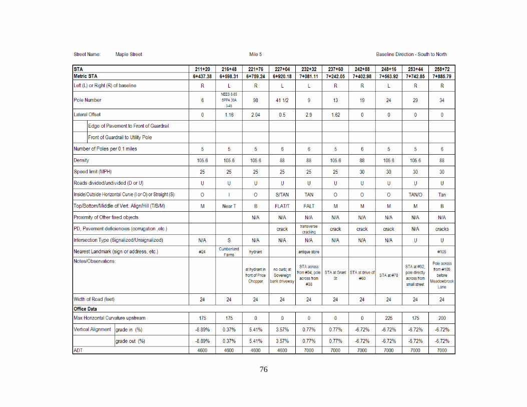
76

77

78

79

80
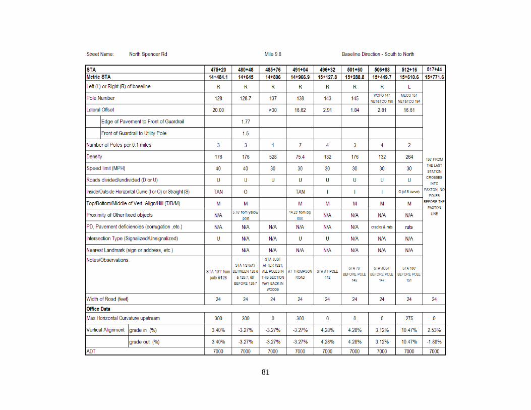
81

Appendix C – Average Lateral Offset Data Collection Sheets

83

84

85

86
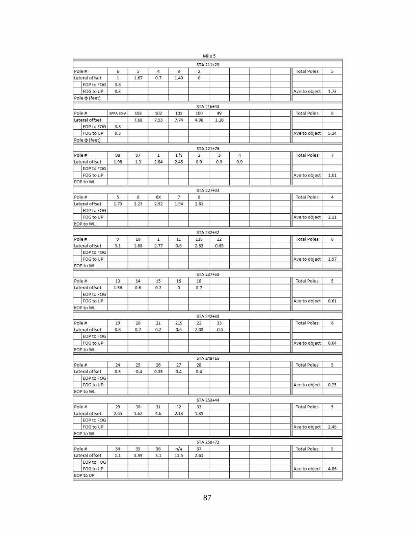
87
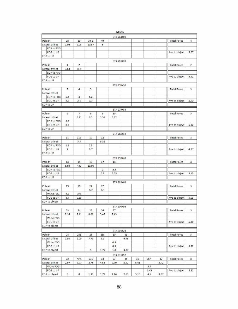
88

89

90

91
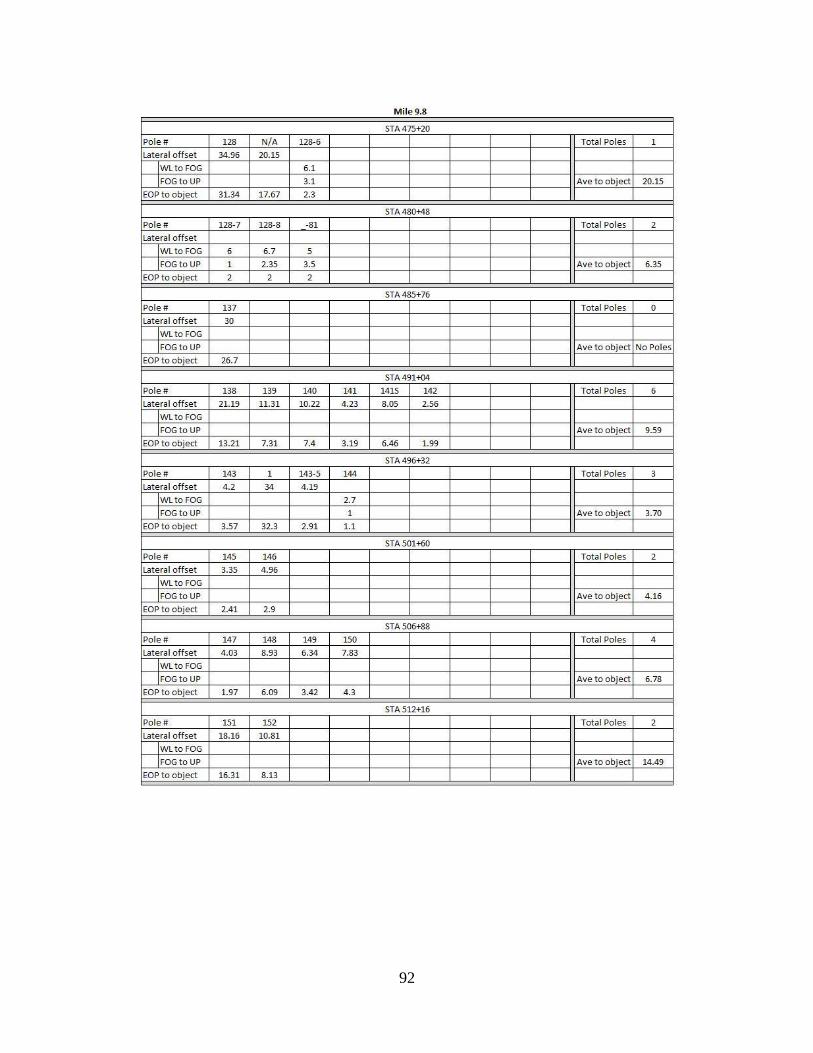
92
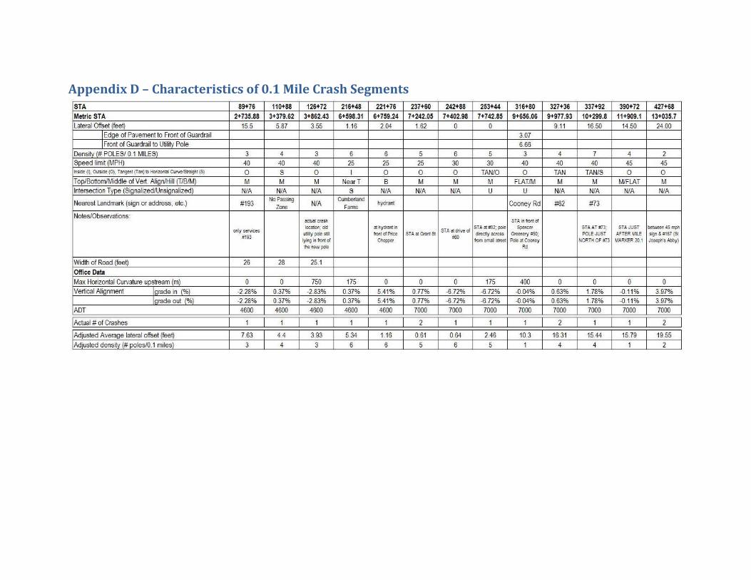
Appendix D – Characteristics of 0.1 Mile Crash Segments

94
Appendix E – Summary of Characteristics of 1 mile Crash Segments
STA Mile 1 Mile 2 Mile 3 Mile 4 Mile 5 Mile 6 Mile 7 Mile 8 Mile 9 Mile 9.8
Number of Poles per 1 mile 33 37 38 37 54 42 43 34 17 34
Ave. Speed limit (MPH) 40 40 40 33 27 39 40 45 42 32
Average Horizontal Curvature (feet) 639.8 897.3 246.1 209.6 311.7 811.1 0.0 508.5 180.4 481.9
Absolute Average Grade 0.00369 0.006692 0.006917 0.01268 0.023771 0.00717 0.011867 0.010442 0.030313 0.019675
Average AADT 4600 4600 4600 4600 6040 7000 7000 7000 7000 7000
Average lateral offset to object (feet) 6.61 9.01 5.78 3.65 2.16 5.21 11.26 12.10 15.31 9.32
ENGLISH UNITS

95
Appendix F – Summary of Data for Segments determined by Road Characteristics

96
Segment
STA 00+00 05+28 10+56 15+84 21+12 26+40 31+68 36+96 42+24 47+52 52+80 58+08 AVE
Number of Poles per 0.1 mile 3 4 3 3 4 5 3 3 5 2 5 6 3.8
Speed limit (MPH) 40 40 40 40 40 40 40 40 40 40 40 40 40
Horizontal Curvature (feet) 0 0 0 1722 0 1476 0 1558 0 1640 2001 1640 837
Vertical Alignment |grade| -0.0439 0.0199 0.0199 0.0199 0.0199 -0.0186 -0.0186 -0.0186 0.0285 0.0285 0.0285 0.0285 0.0078
ADT 4600 4600 4600 4600 4600 4600 4600 4600 4600 4600 4600 4600 4600
Average lateral offset to object (feet) 3.24 5.50 5.07 7.17 8.83 9.18 5.93 8.47 7.48 5.25 9.56 12.23 7.32
TOTAL
Actual # of Crashes 0 0 0 0 0 0 0 0 0 0 0 0 0
Segment
STA 63+36 68+64 73+92 79+20 84+48 89+76 95+04 100+32 105+60 110+88 116+16 121+44 126+72 132+00 137+28 142+56
Number of Poles per 0.1 mile 2 3 3 5 4 3 4 2 3 4 5 2 3 3 4 4
Speed limit (MPH) 40 40 40 40 40 40 40 40 40 40 40 40 40 40 40 40
Horizontal Curvature (feet) 0 984 984 0 984 0 1230 1148 0 0 0 0 2461 0 0 0
Vertical Alignment |grade| -0.0158 -0.0158 -0.0572 0.0321 -0.0228 -0.0228 -0.0053 -0.0267 0.0253 0.0037 0.0638 -0.0283 -0.0283 -0.0283 -0.0164 -0.0164
ADT 4600 4600 4600 4600 4600 4600 4600 4600 4600 4600 4600 4600 4600 4600 4600 4600
Average lateral offset to object (feet) 8.80 12.00 12.90 6.77 8.50 7.63 6.75 4.90 5.37 4.40 4.55 6.10 3.93 4.00 6.35 10.40
Actual # of Crashes 0 0 0 0 0 1 0 0 0 1 0 0 1 0 0 0
Segment
STA 147+84 153+12 158+40 163+68 168+96 174+24 179+52 AVE
Number of Poles per 0.1 mile 6 4 3 4 2 4 5 3.6
Speed limit (MPH) 40 40 40 40 40 40 40 40
Horizontal Curvature (feet) 0 0 0 0 0 0 0 487
Vertical Alignment |grade| -0.0164 -0.0281 -0.0524 -0.0524 0.0447 0.0435 0.0306 -0.0100
ADT 4600 4600 4600 4600 4600 4600 4600 4600
Average lateral offset to object (feet) 7.32 5.38 3.93 5.08 6.20 7.01 6.17 7.08
TOTAL
Actual # of Crashes 0 0 0 0 0 0 0 3
Segment
STA 184+80 190+08 195+36 200+64 205+92 211+20 216+48 221+76 227+04 232+32 237+60 242+88 248+16 253+44 258+72 AVE
Number of Poles per 0.1 mile 4 4 5 4 5 5 5 5 6 6 5 6 5 5 6 5.07
Speed limit (MPH) 40 25 25 25 25 25 25 25 25 25 25 30 30 30 30 27
Horizontal Curvature (feet) 0 820 0 1066 0 574 574 0 0 0 0 0 738 574 656 334
Vertical Alignment |grade| -0.0171 0.0398 -0.0621 -0.0125 -0.0889 -0.0889 0.0037 0.0541 0.0357 0.0077 0.0077 -0.0672 -0.0672 -0.0672 -0.0672 -0.0260
ADT 4600 4600 4600 4600 4600 4600 4600 4600 4600 7000 7000 7000 7000 7000 7000 5560
Average lateral offset to object (feet) 2.89 1.77 1.39 0.55 1.84 1.73 5.33 1.61 2.10 2.00 0.61 0.64 0.25 2.46 4.86 2.00
TOTAL
Actual # of Crashes 0 0 0 0 0 0 1 1 0 0 2 1 0 1 0 6
1
2
2
3
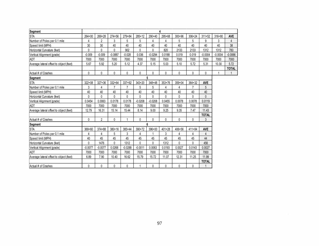
97
Segment
STA 264+00 269+28 274+56 279+84 285+12 290+40 295+68 300+96 306+24 311+52 316+80 AVE
Number of Poles per 0.1 mile 4 2 3 5 5 4 4 5 5 9 3 4
Speed limit (MPH) 30 30 40 40 40 40 40 40 40 40 40 38
Horizontal Curvature (feet) 0 0 0 902 0 0 820 2133 2133 1312 1312 783
Vertical Alignment |grade| -0.009 -0.009 -0.0887 -0.028 0.036 -0.0294 0.0188 0.019 0.019 -0.0004 -0.0004 -0.0066
ADT 7000 7000 7000 7000 7000 7000 7000 7000 7000 7000 7000 7000
Average lateral offset to object (feet) 5.67 5.92 5.20 5.12 4.37 5.15 5.03 5.10 5.72 5.31 10.30 5.72
TOTAL
Actual # of Crashes 0 0 0 0 0 0 0 0 0 0 1 1
Segment
STA 322+08 327+36 332+64 337+92 343+20 348+48 353+76 359+04 364+32 AVE
Number of Poles per 0.1 mile 3 4 7 7 5 5 4 4 7 5
Speed limit (MPH) 40 40 40 40 40 40 40 40 40 40
Horizontal Curvature (feet) 0 0 0 0 0 0 0 0 0 0
Vertical Alignment |grade| 0.0454 0.0063 0.0178 0.0178 -0.0208 -0.0208 0.0455 0.0078 0.0078 0.0119
ADT 7000 7000 7000 7000 7000 7000 7000 7000 7000 7000
Average lateral offset to object (feet) 12.79 16.31 15.14 15.44 8.14 9.00 9.25 9.35 7.47 11.43
TOTAL
Actual # of Crashes 0 2 0 1 0 0 0 0 0 3
Segment
STA 369+60 374+88 380+16 385+44 390+72 396+00 401+28 406+56 411+84 AVE
Number of Poles per 0.1 mile 4 4 5 3 4 1 3 4 4 4
Speed limit (MPH) 40 45 45 45 45 45 45 45 45 44
Horizontal Curvature (feet) 0 1476 0 1312 0 0 1312 0 0 456
Vertical Alignment |grade| -0.0077 -0.0077 0.0268 -0.0288 -0.0011 0.0063 0.0193 0.0027 0.0143 0.0027
ADT 7000 7000 7000 7000 7000 7000 7000 7000 7000 7000
Average lateral offset to object (feet) 6.89 7.90 10.40 16.62 15.79 15.72 11.07 12.31 11.25 11.99
TOTAL
Actual # of Crashes 0 0 0 0 1 0 0 0 0 1
4
5
6
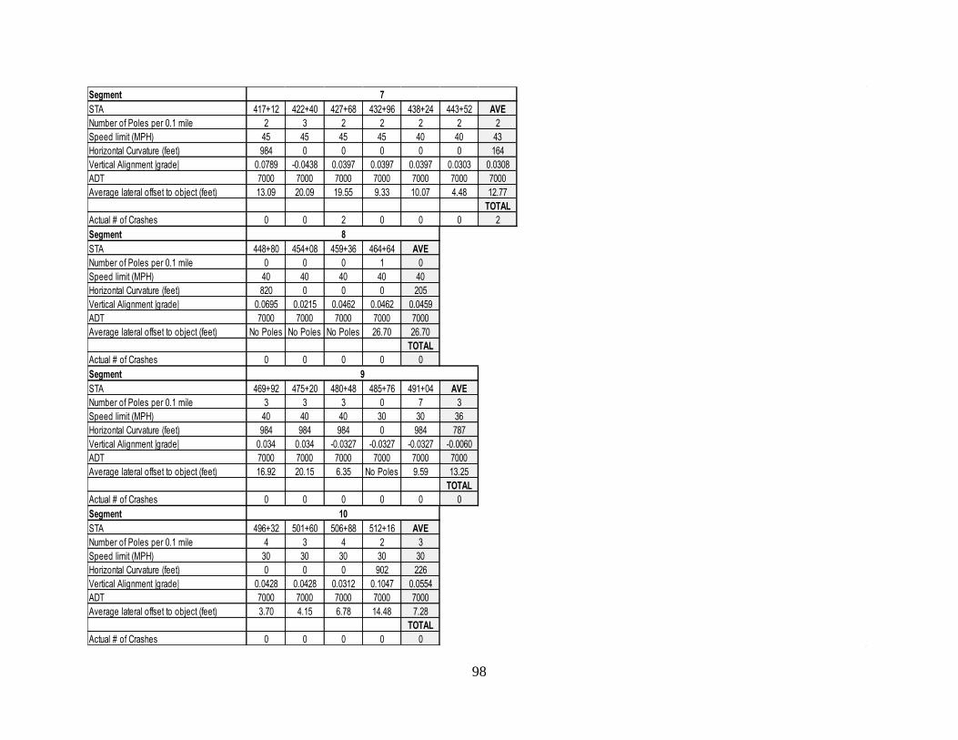
98
Segment
STA 417+12 422+40 427+68 432+96 438+24 443+52 AVE
Number of Poles per 0.1 mile 2 3 2 2 2 2 2
Speed limit (MPH) 45 45 45 45 40 40 43
Horizontal Curvature (feet) 984 0 0 0 0 0 164
Vertical Alignment |grade| 0.0789 -0.0438 0.0397 0.0397 0.0397 0.0303 0.0308
ADT 7000 7000 7000 7000 7000 7000 7000
Average lateral offset to object (feet) 13.09 20.09 19.55 9.33 10.07 4.48 12.77
TOTAL
Actual # of Crashes 0 0 2 0 0 0 2
Segment
STA 448+80 454+08 459+36 464+64 AVE
Number of Poles per 0.1 mile 0 0 0 1 0
Speed limit (MPH) 40 40 40 40 40
Horizontal Curvature (feet) 820 0 0 0 205
Vertical Alignment |grade| 0.0695 0.0215 0.0462 0.0462 0.0459
ADT 7000 7000 7000 7000 7000
Average lateral offset to object (feet) No Poles No Poles No Poles 26.70 26.70
TOTAL
Actual # of Crashes 0 0 0 0 0
Segment
STA 469+92 475+20 480+48 485+76 491+04 AVE
Number of Poles per 0.1 mile 3 3 3 0 7 3
Speed limit (MPH) 40 40 40 30 30 36
Horizontal Curvature (feet) 984 984 984 0 984 787
Vertical Alignment |grade| 0.034 0.034 -0.0327 -0.0327 -0.0327 -0.0060
ADT 7000 7000 7000 7000 7000 7000
Average lateral offset to object (feet) 16.92 20.15 6.35 No Poles 9.59 13.25
TOTAL
Actual # of Crashes 0 0 0 0 0 0
Segment
STA 496+32 501+60 506+88 512+16 AVE
Number of Poles per 0.1 mile 4 3 4 2 3
Speed limit (MPH) 30 30 30 30 30
Horizontal Curvature (feet) 0 0 0 902 226
Vertical Alignment |grade| 0.0428 0.0428 0.0312 0.1047 0.0554
ADT 7000 7000 7000 7000 7000
Average lateral offset to object (feet) 3.70 4.15 6.78 14.48 7.28
TOTAL
Actual # of Crashes 0 0 0 0 0
10
7
8
9