Computational Statistics and Data Analysis 80 (2014) 57–69

Contents lists available at ScienceDirect

Computational Statistics and Data Analysis

journal homepage: www.elsevier.com/locate/csda

Evaluation of the Fisher information matrix in nonlinearmixed effect models using adaptive Gaussian quadratureThu Thuy Nguyen ∗, France MentréIAME, UMR 1137, INSERM, F-75018 Paris, FranceUniversity Paris Diderot, Sorbonne Paris Cité, F-75018 Paris, France

a r t i c l e i n f o

Article history:Received 9 October 2013Received in revised form 9 June 2014Accepted 10 June 2014Available online 17 June 2014

Keywords:DesignDose–response studiesFisher information matrixAdaptive Gaussian quadratureLinearisationNonlinear mixed effect model

a b s t r a c t

Nonlinear mixed effect models (NLMEM) are used in model-based drug development toanalyse longitudinal data. To design these studies, the use of the expected Fisher informa-tion matrix (MF ) is a good alternative to clinical trial simulation. Presently, MF in NLMEMis mostly evaluated with first-order linearisation. The adequacy of this approximation is,however, influenced by model nonlinearity. Alternatives for the evaluation of MF with-out linearisation are proposed, based on Gaussian quadratures. The MF , expressed as theexpectation of the derivatives of the log-likelihood, can be obtained by stochastic integra-tion. The likelihood for each simulated vector of observations is approximated by Gaussianquadrature centred at 0 (standard quadrature) or at the simulated random effects (adap-tive quadrature). These approaches have been implemented in R. Their relevancewas com-pared with clinical trial simulation and linearisation, using dose–response models, withvarious nonlinearity levels and different number of doses per patient. When the nonlin-earity was mild, three approaches based onMF gave correct predictions of standard errors,when compared with the simulation. When the nonlinearity increased, linearisation cor-rectly predicted standard errors of fixed effects, but over-predicted, with sparse designs,standard errors of some variability terms. Meanwhile, quadrature approaches gave correctpredictions of standard errors overall, but standard Gaussian quadrature was very time-consuming when there were more than two random effects. To conclude, adaptive Gaus-sian quadrature is a relevant alternative for the evaluation of MF for models with strongernonlinearity, while being more computationally efficient than standard quadrature.

© 2014 Elsevier B.V. All rights reserved.

1. Introduction

Nonlinear mixed effect models (NLMEM) are frequently used in model-based drug development to analyse longitu-dinal data obtained during clinical trials (Lalonde et al., 2007; Smith and Vincent, 2010). They were introduced about40 years ago (Sheiner et al., 1972, 1977) and were initially used in pharmacokinetic analyses as an alternative to the non-compartmental approach (NCA) (Gabrielson and Weiner, 2006). This modelling approach is more complex than NCA, butallows for the analysis of few samples per subject. It accounts for within and between subject variability, and is appropriatefor exploiting the richness of repeated measurements. Consequently, this approach is increasingly used in the biomedi-cal field, not only for pharmacokinetic analyses (Sheiner et al., 1972, 1977), but also for analyses of viral loads (Perelsonand Ribeiro, 2008), of bacterial resistance to antibiotics (Nielsen et al., 2007), and of the dose–response relationship. This

∗ Correspondence to: IAME, UMR 1137, INSERM - University Paris Diderot, 16 Henri Huchard, 75018, Paris, France. Tel.: +33 157277540.E-mail address: thu-thuy.nguyen@inserm.fr (T.T. Nguyen).

http://dx.doi.org/10.1016/j.csda.2014.06.0110167-9473/© 2014 Elsevier B.V. All rights reserved.

58 T.T. Nguyen, F. Mentré / Computational Statistics and Data Analysis 80 (2014) 57–69

approach has become themain statistical tool in pharmacometrics, the science of quantitative pharmacology (Vander Graaf,2012). Parameters of these models are commonly estimated by likelihood maximisation (Dartois et al., 2007). However, thenonlinearity of the structural model prevents a closed form solution for the integration over the random effects in the ex-pression of the likelihood function. Many approaches have been proposed over the years to overcome this difficulty, andimplemented in several estimation software packages. These are first-order marginal quasi-likelihood or first-order lineari-sation (Lindstrom and Bates, 1990) in NONMEM, R, Splus, Laplace approximation (Wolfinger, 1993) in NONMEM and SAS,adaptive Gaussian quadrature (Pinheiro and Bates, 1995) in SAS and in the R package lme4, Stochastic Approximation Ex-pectation Maximisation (SAEM) (Kuhn and Lavielle, 2005) in MONOLIX and NONMEM. Pillai et al. (2005) described theseestimation methods in a review paper and recently, Plan et al. (2012) compared their performance, showing that adaptiveGaussian quadrature, although the slowest, was generally the best method.

Before themodelling step to estimate parameters, it is important to define an appropriate design,which consists in deter-mining a balance between the number of subjects and the number of samples per subject, as well as the allocation of timesand doses, according to experimental conditions. The choice of design is crucial for an efficient estimation of model param-eters (Al-Banna et al., 1990; Hashimoto and Sheiner, 1991; Jonsson et al., 1996), especially when the studies are conductedin children or in patients where only a few samples can be taken per subject. The main approach for design evaluation haslong been based on clinical trial simulation (CTS), but it is a cumbersome method and so the number of designs that canbe evaluated is limited. An alternative approach has been described in the general theory of optimum experimental designused for classical nonlinear models (Atkinson et al., 2007; Walter and Pronzato, 2007; Atkinson et al., 2014), relying on theRao–Cramer inequality which states that the inverse of the Fisher information matrix (MF ) is the lower bound of the vari-ance–covariance matrix of any unbiased estimate of the parameters and its diagonal elements are the expected variances ofthe parameters. Several criteria based onMF have been developed to evaluate designs. One of the criteria widely used is thecriterion of D-optimality, which consists in maximising the determinant of MF . The computation of this criterion requiresa priori knowledge of the model and its parameters, which can usually be obtained from previous experiments. This leadsto the concept of ‘‘locally optimal designs’’, which has been studied in several publications (Chernoff, 1953; Box and Lucas,1959; D’Argenio, 1981). Since there is no closed form of the likelihood in NLMEM, there is no analytical expression of MF .An approximation of the expectedMF has been proposed for NLMEM, using first order linearisation of themodel around therandomeffect expectation (Mentré et al., 1997; Retout et al., 2002; Bazzoli et al., 2009). This approach has been implementedin several software programs (Bazzoli et al., 2010; Leonov and Aliev, 2012; Gueorguieva et al., 2007; Nyberg et al., 2012) suchas PFIM (INSERM, University Paris Diderot), POPED (University of Uppsala), POPDES (University of Manchester), and POPT(University of Otago), frequently used to design new studies in academia as well as in pharmaceutical companies (Mentréet al., 2013).

However, it has been shown that the use of the linearisation (LIN) approach is only appropriate if the variances of therandom effects are small, or the nonlinearity is mild (Jones and Wang, 1999; Jones et al., 1999). Consequently, as pointedout by Han and Chaloner (2005), when an optimal design is found using this approximation but the estimation is carried outusing a true NLMEM, the performance of the design needs further investigation. The nonlinearity of a model with respectto its parameters is defined from the behaviour of the first order derivatives of the model function. Its consequences on thestructural identifiability of a model have been studied by Walter and Pronzato (1995). The notion of level of nonlinearity(‘‘mild’’ or ‘‘strong’’ as mentioned in this paper) is derived from the term ‘‘close to linear’’ introduced when evaluating anonlinear model’s behaviour (Fletcher and Powell, 1963). Measures of nonlinearity have been studied in several publica-tions (Bates and Watts, 1980; Cook and Goldberg, 1986; Smyth, 2002) in order to evaluate whether the ‘‘close to linear’’condition is satisfied and to indicate if the linear approximation is reasonable or questionable. When first-order linearisa-tion is to be avoided, alternative approaches are necessary. Various new approaches have been proposed, but these are notalways better than the usual first-order linearisation. For instance, linearisation of themodel around the individual values ofthe random effects (Retout and Mentré, 2003) or around the expected mode of the marginal likelihood (Nyberg et al., 2012)has been proposed but is quite time consuming becauseMonte Carlo simulations are needed. Other approaches based on theLaplace approximation (Vong et al., 2012) or Monte Carlo integration (Mielke, 2012) give correct predictions for the preci-sion of parameter estimation, but they are also very time consuming. Another possible alternative for computing the Fisherinformation matrix in designing studies is the use of Gaussian quadrature rules. This consists in approximating integrals offunctions with respect to a given probability density by a weighted sum of function values at abscissas chosen within theintegration domain. It has been shown that adaptive Gaussian quadrature (AGQ) performs better than standard Gaussianquadrature (GQ) in estimation (Pinheiro and Bates, 1995); the difference between the two approaches is that the grid ofnodes is centred at the expectation of the random effects in GQ while it is centred at the conditional modes of the randomeffects in AGQ. Neither approach has ever been proposed for designing studies with different types of models, except in anexample of an HIV dynamic model written with ordinary differential equations (Guedj et al., 2007).

In this context, we aim to propose alternatives to linearisation for evaluating the predicted Fisher information matrix,based on GQ and AGQ. In order to challenge and investigate the performance of both new approaches as well as linearisationcompared with CTS, we use examples of dose–response trials inspired by the article of Plan et al. (2012) comparingdifferent estimationmethods. Dose–response studies are of critical importance in drug development and need to be plannedcarefully (Bretz et al., 2010; Pronzato, 2010; McGree et al., 2012) but little has been done to study their design in the contextofNLMEM.We consider the sigmoid Emax model,with various degrees of nonlinearity (i.e. different sigmoidicity coefficients),and in addition a linear model whereMF can be calculated exactly.

T.T. Nguyen, F. Mentré / Computational Statistics and Data Analysis 80 (2014) 57–69 59

We introduce the necessary notation for the design and model and present the new GQ and AGQ approaches developedfor computingMF in Section 2. The performance of both approaches is evaluated and comparedwith CTS and LIN for differentscenarios in Section 3 and is discussed in Section 4.

2. Computing Fisher information matrix in NLMEMwith Gaussian quadratures

2.1. Design

The elementary design ξi of individual i (i = 1, . . . ,N) is defined by the number ni of observations and the designvariables (xi1, . . . , xini). Consequently, the population design for N individuals can be defined as Ξ = ξ1, . . . , ξN. Usually,population designs are composed of a limited number Q of groups of individuals with identical designs in each group. Eachof these groups is composed of a global elementary design ξq and is performed in a number Nq of subjects. The populationdesign can thus be written as Ξ = [ξ1,N1]; . . . ; [ξQ ,NQ ].

2.2. Nonlinear mixed effect model

We denote by yi the ni-vector of observations for the individual i obtainedwith the design ξi and by f the known functiondescribing the nonlinear structural model. The NLMEM linking the response yi to the samples ξi = (xi1, . . . , xini) can bewritten as

yi = f (φi, ξi) + εi, (1)

where εi is the vector of random errors which follows a standard normal distributionN (0, σ 2Ini) and Ini is an ni ×ni identitymatrix. The vector of individual parameters φi can be expressed as function g of µ, the P-vector of fixed effects and of bi,the P-vector of random effects for individual i. g can be additive (for normal parameters), so that the pth component of φi iswritten as

φip = g(µp, bip) = µp + bip, (2)

or exponential (for lognormal parameters), so

φip = g(µp, bip) = µp exp(bip). (3)

It is assumed that bi ∼ N (0, Ω), withΩ definedhere as a diagonal variance–covariancematrix of size P×P . Each elementω2p

ofΩ represents the variance of the pth component of bi. As usual, the following assumptions aremade: εi|bi are independentbetween subjects, and εi and bi are independent for each subject. The model can also be written as

yi = f (g(µ, bi), ξi) + εi. (4)

Let λ = (ω1, . . . , ωP , σ )′ be the vector of standard deviations of random effects and standard deviation of random error. Ψ ,the vector of all population parameters to be estimated, is Ψ = (µ′, λ′)′.

2.3. Fisher information matrix

The individual Fisher information matrix is defined from the likelihood of the observations yi of individual i, which isexpressed by the following integral:

L(yi; Ψ ) =

RP

p(yi|bi; Ψ ) p(bi) dbi, (5)

where p(yi|bi; Ψ ) is the conditional density of the observations yi given the random effects bi, and p(bi) is the density ofbi ∼ N (0, Ω). Then, the Fisher information matrix for the elementary design ξi is the following expectation taken withrespect to the distribution of the observations p(y; Ψ )

MF (Ψ ; ξi) = E

∂ log L(yi; Ψ )

∂Ψ

∂ log L(yi; Ψ )

∂Ψ

′

. (6)

As the individuals are independent, the Fisher information matrix MF (Ψ , Ξ) for a population design Ξ is defined by thesum of the N elementary matricesMF (Ψ , ξi), so that

MF (Ψ , Ξ) =

Ni=1

MF (Ψ , ξi). (7)

In the case of a limited number Q of elementary designs ξq, we have

MF (Ψ , Ξ) =

Qq=1

NqMF (Ψ , ξq). (8)

60 T.T. Nguyen, F. Mentré / Computational Statistics and Data Analysis 80 (2014) 57–69

However, there is no analytical expression for the likelihood L(yi; Ψ ) in NLMEM. Approximations such as linearisation can beused to approximate the Fisher informationmatrix (Mentré et al., 1997; Retout et al., 2002; Bazzoli et al., 2009). ThepredictedMF after linearisation is a block matrix with a block corresponding to derivatives of the log-likelihood with respect to thefixed effects, a block for derivatives with respect to the standard derivation terms and a block containing mixed derivativeswith respect to all parameters. In ourwork, the block ofmixed derivativeswas set to 0 for linearisation, based on publicationsshowing the better performance of the block diagonal expression compared with the full one (Mielke and Schwabe, 2010;Fedorov and Leonov, 2014; Nyberg et al., 2014).

2.4. Gaussian quadrature and adaptive Gaussian quadrature

When linearisation is to be avoided, alternatives such as Gaussian quadratures can be used to express the likelihoodanalytically. For simplicity, we omit the index i for the individual in this section. The elementary Fisher information matrixMF (Ψ , ξ) in (6) for an individual with elementary design ξ of n observations can also be written as

MF (Ψ , ξ) =

Rn

h(y; Ψ ) p(y; Ψ ) dy, (9)

where p(y; Ψ ) is the marginal density of y and

h(y; Ψ ) =∂ log L(y; Ψ )

∂Ψ

∂ log L(y; Ψ )

∂Ψ ′=

∂L(y;Ψ )

∂Ψ

∂L(y;Ψ )

∂Ψ ′

L(y; Ψ )2. (10)

First, we propose to evaluate the integral of h(y; Ψ ) with respect to p(y; Ψ ) in (9) by stochastic integration. We generateM vectors of observations ym (m = 1, . . . ,M), each vector with the same design ξ of n samples, under the same probabilitydistribution p(y; Ψ ). Thus, an approximation of (9) can be obtained by

MF (Ψ , ξ) =1M

Mm=1

h(ym; Ψ ). (11)

Then, in order to obtain an analytical expression of h(ym; Ψ ) as expressed in (10) for each simulated ym, we need tocompute the likelihood L(ym; Ψ ). We define η = Ω−1/2b, then η ∼ N (0, IP), where IP is the identity matrix of dimensionP × P . Consequently, the likelihood in (5) can also be written as

L(ym; Ψ ) =

RP

p(ym|η; Ψ )p(η)dη, (12)

where p(η) is the density of N (0, IP). This integral can be evaluated numerically by the Gaussian quadrature approach, asa weighted sum of p(ym|η; Ψ ) evaluated at pre-determined nodes chosen within the distribution of η (Pinheiro and Bates,1995). Quadratureweights andnodes for approximating one-dimensional integrals are those of the standardGauss–Hermiterule (Abramowitz and Stegun, 1964;Golub andWelsh, 1969;Golub, 1973). Thenodes are the roots of theHermite polynomialof degree κ , obtained from successive derivatives of exp(η2) (Press et al., 1992). As in Pinheiro and Bates (1995), theP-dimension integral here was transformed into P successive one-dimensional integrals. The distribution of nodes andweights used in standard GQ does not take into account the nature of the integrand, which is why standard GQ requiresa high number of nodes in order to provide a correct estimation of parameters. AGQ, by centring and scaling the standardquadrature nodes, places the nodes according to the areas of high density and improves the approximation. Consequently itrequires fewer nodes comparedwith standard GQ,while giving better performance in estimation (Pinheiro and Bates, 1995).

In order to approximate each one of these integrals in L(ym; Ψ ) using standard GQ, for all simulated ym, κ quadraturenodes and weights are selected from the standard normal distribution N (0, 1). Then the integral of dimension P can beapproximated by the weighted sum over K nodes ηk, where K = κP and ηk are vectors in RP , associated with weights wk(k = 1, . . . , K ). So, we obtain the following analytical expression:

L(ym; Ψ ) =

Kk=1

wk p(ym|ηk; Ψ ), (13)

where ym|ηk ∼ N (fk, σ 2In) with fk = f (g(µ, Ω1/2ηk), ξ). Thus, we can write

p(ym|ηk; Ψ ) = (2πσ 2)−n/2 exp

−12σ 2

(ym − fk)′(ym − fk)

, and (14)

log p(ym|ηk; Ψ ) = −n2log 2π −

n2log σ 2

−1

2σ 2(ym − fk)′(ym − fk). (15)

The likelihood L(ym; Ψ ) can also be approximated by AGQ. Since a vector of standardised random effects ηm is simulatedwhen generating each ym, we select K = κP nodes ηmk and weights wk based onp(η) which is the N (ηm, IP) density. We

T.T. Nguyen, F. Mentré / Computational Statistics and Data Analysis 80 (2014) 57–69 61

can write

L(ym; Ψ ) =

RP

p(ym|η; Ψ )p(η)p(η)p(η)dη (16)

=

Kk=1

wkp(ηmk)p(ηmk)

p(ym|ηmk; Ψ ), (17)

where ym|ηmk ∼ N (fmk, σ2In) with fmk = f (g(µ, Ω1/2ηmk), ξ), and the weights for AGQ can be written as

wkp(ηmk)p(ηmk)

= wk(2π)−P/2 exp(− 1

2η′

mkηmk)

(2π)−P/2 exp(− 12 (ηmk − ηm)′(ηmk − ηm))

(18)

= wk exp

−12

η′

mkηmk − (ηmk − ηm)′(ηmk − ηm)

. (19)

Finally, using (13) or (17) in (10) and in (11), the individual Fisher information matrix can be approximated as

MF (Ψ , ξ) =1M

Mm=1

K

k=1wmk

∂pmk(ym;Ψ )

∂Ψ

K

k=1wmk

∂pmk(ym;Ψ )

∂Ψ ′

Kk=1

wmkpmk(ym; Ψ )

2 (20)

=1M

Mm=1

K

k=1wmkpmk(ym; Ψ )

∂ log pmk(ym;Ψ )

∂Ψ

K

k=1wmkpmk(ym; Ψ )

∂ log pmk(ym;Ψ )

∂Ψ ′

Kk=1

wmkpmk(ym; Ψ )

2 . (21)

When using GQ, wmk = wk and pmk(ym; Ψ ) = p(ym|ηk; Ψ ) as defined in (14). When using AGQ, wmk = wkp(ηmk)p(ηmk)

as definedin (19) and pmk(ym; Ψ ) = p(ym|ηmk; Ψ ) as defined in (14) with fmk instead of fk.

As Ψ = (µ′, λ′)′, the Fisher information matrixMF (Ψ , ξ) can be written as a block matrix

MF (Ψ ; ξ) =

MF (µ; ξ) MF (µ, λ; ξ)

MF (µ, λ; ξ) MF (λ; ξ)

. (22)

To compute MF (µ; ξ), we derive the log-likelihood with respect to each element µp of the vector of fixed effects µ =

(µ1, . . . , µP)′, using

∂ log pmk(ym; Ψ )

∂µp=

1σ 2

∂ fk∂µ′

p(ym − fk), (23)

To computeMF (λ; ξ), we derive the log-likelihoodwith respect to each elementωp or σ of the vector of standard deviationsλ = (ω1, . . . , ωP , σ )′, using

∂ log pmk(ym; Ψ )

∂ωp=

1σ 2

∂ fk∂ω′

p(ym − fk), and (24)

∂ log pmk(ym; Ψ )

∂σ= −

nσ

+1σ 3

(ym − fk)′(ym − fk), (25)

with fmk instead of fk when using AGQ instead of GQ. Finally, using (23)–(25) in (21), we obtain each element of MF (µ; ξ)in (22).

3. Evaluation by simulation

3.1. Evaluation models and scenarios

Our evaluation exampleswere inspired by a previous dose–response simulation study (Plan et al., 2012)whichmimickedclinical trials including 100 subjects with identical individual design ξ and investigating several dose levels among 0, 100,300 and 1000 dose units.

First, we considered a linearmodel of the dose–response relationship describing, for subject i, an effect Eij for the jth dosedij with two structural parameters: baseline E0 and slope S.

Eij = E0i + Si × dij + εij. (26)

62 T.T. Nguyen, F. Mentré / Computational Statistics and Data Analysis 80 (2014) 57–69

Table 1Different models and designs evaluated.Structuralmodel

Number ofparameters P

Number of dosesper subject n

Doses Name

Linear 2 4 (0, 100, 300, 1000) M1R2 (100, 300) M1S

Emax (E0 notestimated, fixedat same value inall subjects)

2γ = 1 4 (0, 100, 300, 1000) M2R

2 (300, 1000) M2S

γ = 3 4 (0, 100, 300, 1000) M3R2 (300, 1000) M3S

Emax (E0estimated,varying betweensubjects)

2γ = 1 4 (0, 100, 300, 1000) M4R

3 (0, 300, 1000) M4S

γ = 3 4 (0, 100, 300, 1000) M5R3 (0, 300, 1000) M5S

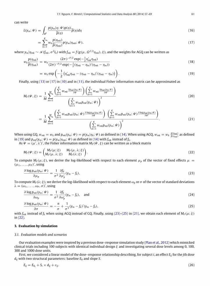
Fig. 1. Individual response versus dose profiles (in grey) for one dataset simulated using linear model (M1R), Emax model with sigmoidicity coefficientγ = 1 (M4R) and Emax model with γ = 3 (M5R), with 4 doses per subject (0, 100, 300, 1000). The black curves represent the response predicted by themodel for the fixed effect parameters.

The vector of the fixed effects µ was composed of µE0 = 5 and µS = 0.06. The random effect model was additive withstandard deviations ωE0 = 1.5 and ωS = 0.018. The standard deviation σ of random error εij was equal to 2. We studiedtwo designs, a rich one ξ = (0, 100, 300, 1000) and a sparse one ξ = (100, 300). We chose to evaluate first a simple linearmixed effect model (denoted by M1) because in this case the analytical form of the Fisher information matrix is known andso we could easily check whether our calculation and implementation are correct.

Next, we considered a sigmoid Emax model of the dose–response relationship, describing for subject i, an effect Eij forthe jth dose dij with the following structural parameters: baseline E0, maximal effect Emax, dose ED50 at which 50% of themaximal effect is achieved and sigmoidicity coefficient γ , i.e. the degree of nonlinearity of the function shape.

Eij = E0i +Emaxi × dγ

ij

EDγ

50i+ dγ

ij+ εij. (27)

We considered amodel with γ = 1 and amodel with γ = 3. In eachmodel, γ was knownwith the same value in all subjects(i.e. µγ not estimated, ωγ = 0). We first studied models with two structural parameters: Emax and ED50 where E0 was fixedat the same value 5 in all subjects (i.e. µE0 not estimated, ωE0 = 0). The fixed effects µ were µEmax = 30, µED50 = 500 andthe random effects were exponential with ωEmax = ωED50 = 0.3. We denote these models M2 and M3 for γ = 1 and γ = 3,respectively. Then, we studied models with three structural parameters: Emax, ED50 and E0, where E0 can vary from onesubject to another and was estimated. The fixed effects µ were µEmax = 30, µED50 = 500, µE0 = 5 and the random effectswere exponential with ωEmax = ωED50 = ωE0 = 0.3. We denote these models M4 and M5 for γ = 1 and γ = 3 respectively.The standard deviation σ of random error εij was equal to 2 in all models. Designs ξ with 2, 3, or 4 doses among (0, 100,300, 1000) were studied. The list of the 5 models above and the designs studied are detailed in Table 1. The rich design isreferred to as R and the sparse design as S. Examples of onedataset simulatedusing linearmodel, Emax modelwith 3 structuralparameters, γ = 1 or γ = 3 and the rich design of 4 doses per subject (M1R,M4R andM5R respectively) are plotted in Fig. 1.

We plotted the first and second order derivatives to examine graphically the model nonlinearity (Fig. 2). The first deriva-tives with respect to Emax and ED50 vary over design samples and are presented in Fig. 2A.We notice that the derivative with

T.T. Nguyen, F. Mentré / Computational Statistics and Data Analysis 80 (2014) 57–69 63

(A) First order derivatives.

(B) Second order derivatives.

Fig. 2. First order (panel A) and second order (panel B) derivatives of the function f of the Emax model with respect to the structural parameters Emax andED50 for two sigmoidicity coefficients γ = 1 and γ = 3.

respect to Emax depends on ED50 and the one with respect to ED50 depends on both Emax and ED50. Thus the optimal designdepends on values of Emax and ED50 but not on E0. One class of nonlinearity measures is based on the second order deriva-tives (Smyth, 2002): if the second derivatives of model f1 are smaller in absolute values than f2, then model f1 has ‘‘closer tolinear’’ behaviour. The second derivatives that are different from 0 are plotted against doses in Fig. 2B. The magnitudes ofthe curves are greater when γ = 3 than when γ = 1, indicating that model nonlinearity increases with γ . This observationwas confirmed by Plan et al. (2012) who showed decreasing performance of the linearisation approach along the γ -increasewhen estimating parameters for Emax models.

3.2. Comparison of standard errors between predictions and clinical trial simulation

Our aim was to evaluate and compare the standard errors (SE) predicted using MF by GQ and AGQ with those obtainedby CTS and LIN.

64 T.T. Nguyen, F. Mentré / Computational Statistics and Data Analysis 80 (2014) 57–69

Fig. 3. Relative standard error RSE (%) for the linear dose–response model obtained by clinical trial simulation (white bar) versus those predicted bylinearisation (light grey bar), Gaussian quadrature (dark grey bar) and adaptive Gaussian quadrature (black bar), for the fixed effects (µ), the standarddeviation of the random effects (ω), and of the random error (σ ), with rich or sparse designs: M1R (4 doses per subject), M1S (2 doses per subject). The95% confidence intervals of the RSE obtained by clinical trial simulation are displayed on top of the white bars.

We performed clinical trial simulations in R 2.14.1 with the model, parameters and designs above. For each scenario,1000 datasets of 100 subjects were simulated. Each simulated dataset was then analysed in MONOLIX 3.2 (www.lixoft.eu).Population parameters were estimated by the SAEM algorithm (Kuhn and Lavielle, 2005). Next, the SE by CTS, defined asthe unbiased sample estimate of the standard deviation from the 1000 parameter estimates, were calculated. The relativestandard errors (RSE) byCTSwere defined as the ratio of the SE to the true value of parameters. As in the publication byRetout

and Mentré (2003), the 95% confidence intervals for each RSE by CTS are given, computed as

q1999RSE

2;

q2999RSE

2

where q1 and q2 are, respectively, the 2.5% and 97.5% quantiles of the χ2 distribution with 999 degrees of freedom. Wealso computed the determinant of the variance–covariance matrix of all parameter estimates, normalised according to thestandard definition of D-criterion, i.e. det(MF )

−1/(2P+1).In parallel, we first used PFIM 3.2.2 (www.pfim.biostat.fr) with the model, parameters and designs above to predict MF

by LIN. Second, we implemented the calculations for GQ and AGQ (Section 2.4) in R 2.14.1 in a working version of PFIM,using the function gauss.quad.prob of the R package statmod and the function as.weight of the R package plink formultidimensional quadratures, which is an extension of gauss.quad.prob. We used M = 1000 simulations to computethe expectation of h (see Eq. (11)). We found that κ = 100 nodes are needed for GQ and only 30 nodes for AGQ to guaranteestable results with all studied models. The predicted SE of parameters were calculated as the square root of the diagonalterms of M−1

F and the predicted RSE were defined as the ratio of the SE to the true value of parameters. We also calculatedthe normalised determinant of the predicted variance–covariance matrix of parameter estimates (as defined above).

Finally, we compared the RSE and the normalised determinant of the variance–covariance matrix predicted using LIN,GQ and AGQ with those obtained by CTS.

3.3. Results

For the linear dose–response model (Fig. 3), the RSE predicted by LIN, GQ and AGQ were close and in the same range asthe ones calculated from CTS. In this case, the linearisation approach provided the exact calculation ofMF and of the true SE.As expected, the RSE were higher in the sparse design with 2 doses (Fig. 3, M1S) than in the rich design with 4 doses (Fig. 3,M1R), not so much for the fixed effects but more for the standard deviations of the random effects and of the random error.

For the Emax model with 2 structural parameters and 2 random effects, when γ = 1 (Fig. 4, M2R–M2S), the three predic-tion approaches gave RSE close to those obtained by CTS. However, when γ = 3 (Fig. 4, M3R–M3S), with the sparse design,the linearisation approach over-predicted the RSE for ωED50 and especially for σ (42% predicted by LIN versus 15% by GQ,14% by AGQ and 17% obtained by CTS). With the rich design, the level of nonlinearity seemed to have less impact on theperformance of linearisation: like GQ and AGQ, LIN adequately predicted RSE of all model parameters, in the same range asthe ones obtained by CTS.

For the Emax model with 3 structural parameters and 3 random effects, when γ = 1 (Fig. 5, M4R–M4S), the three pre-diction approaches gave RSE in the same range as those obtained by CTS. However, as in the previous model, when γ = 3(Fig. 5, M5R–M5S), the performance of the linearisation approach deteriorated with the sparse design and it over-predictedthe RSE ofωE0 (27% predicted by LIN versus 19% by GQ, 21% by AGQ and 20% obtained by CTS). With the rich design, the fourapproaches gave RSE that were close.

It is of note, as reported in Figs. 3–5, that the RSE obtained by CTS were representative of the true RSE because rathersmall 95% confidence intervalswere found. Fig. 6 represents the normalised determinants of the variance–covariancematrixobtained by the four approaches for different scenarios. Overall, the predicted variances were lower than the ones observedfrom CTS. However, for the scenario M3S, LIN predicted a determinant of the variance–covariance matrix that is larger thanthe one obtained by CTS.

Regarding computing time, the linearisation approach was much faster than the two other prediction approaches. Forthe models with 2 random effects, the runtimes were less than 1 s by LIN in PFIM 3.2.2, about 6 h by GQ, 20 min by AGQ,

T.T. Nguyen, F. Mentré / Computational Statistics and Data Analysis 80 (2014) 57–69 65

Fig. 4. Relative standard error RSE (%) for the Emax dose–response model with fixed baseline, obtained by clinical trial simulation (white bar) versus thosepredicted by linearisation (light grey bar), Gaussian quadrature (dark grey bar) and adaptive Gaussian quadrature (black bar), for the fixed effects (µ), thestandard deviation of the random effects (ω), and of the random error (σ ), with rich or sparse designs: M2R (γ = 1, 4 doses per subject), M2S (γ = 1, 2doses per subject), M3R (γ = 3, 4 doses per subject), M3S (γ = 4, 2 doses per subject). The 95% confidence intervals of the RSE obtained by clinical trialsimulation are displayed on top of the white bars.

Fig. 5. Relative standard error RSE (%) for the Emax dose–response model with estimated baseline, obtained by clinical trial simulation (white bar) versusthose predicted by linearisation (light grey bar), Gaussian quadrature (dark grey bar) and adaptive Gaussian quadrature (black bar), for the fixed effects(µ), the standard deviation of the random effects (ω), and of the random error (σ ), with rich or sparse designs: M4R (γ = 1, 4 doses per subject), M4S(γ = 1, 3 doses per subject), M5R (γ = 3, 4 doses per subject), M5S (γ = 4, 3 doses per subject). The 95% confidence intervals of the RSE obtained byclinical trial simulation are displayed on top of the white bars.

Fig. 6. Determinant of the variance–covariancematrix of parameter estimates, normalised by inverse of the total number of parameters (2P+1), obtainedby clinical trial simulation (white bar) versus those predicted by linearisation (light grey bar), Gaussian quadrature (dark grey bar) and adaptive Gaussianquadrature (black bar), for different models as defined in Table 1.

66 T.T. Nguyen, F. Mentré / Computational Statistics and Data Analysis 80 (2014) 57–69

and 10 h by CTS. For the models with 3 random effects, the runtimes were less than 1 s by LIN, about 110 h by GQ, 11 h byAGQ and 12 h by CTS.

4. Discussion

The presentwork proposes new approaches to the evaluation of the Fisher informationmatrix in NLMEM, using Gaussianquadrature and adaptive Gaussian quadrature when designing longitudinal studies. This is an alternative to first-order lin-earisation, the most commonly used approach in the field of optimal design in NLMEM.We investigated the performance ofthese approaches in predicting parameter standard errors and determinants of the Fisher matrix for dose–response models,as compared with linearisation and clinical trial simulation. These predictions are important for design evaluation which isalways the first step when planning an upcoming study and correct values of the D-criterion are needed for design optimi-sation.

When the nonlinearity was mild (γ = 1), the linearisation approach gave correct predictions of the RSE, close to theempirical ones obtained by simulation. When nonlinearity increased (γ = 3), linearisation correctly predicted the RSE offixed effects but over-predicted, in the case of the sparse design, the RSE of ωED50 and σ . This poor performance could bepartly explained by the behaviour of the first derivatives of the model function, which are used in the calculation of theMFblock corresponding to the standard deviation terms (Bazzoli et al., 2009). As shown in Fig. 2A, the derivatives of f whenγ = 3 (especially with respect to ED50) are much more sensitive to design samples as compared with γ = 1. This mightbe why when γ = 3, with the sparse design of 2 doses (300, 1000) only, RSE of some standard deviation terms were notwell predicted by linearisation. Further evaluations of other examples are needed to understand better the difference inperformance of this approach between the sparse and rich designs.

GQ andAGQgave correct predictions of RSE overall, close to the RSE obtained by CTS, in spite of a slight discrepancy versusCTS for some variability terms. When experimenters design population studies, they are more interested in the magnitudeof the RSE than the exact value, so these approaches are relevant to evaluate MF when linearisation is to be avoided. Here,we used κ = 100 nodes for GQ and κ = 30 nodes for AGQ to approximate the integrals correctly, when compared withCTS, in all studied models (so the total number of model evaluations was K = κP , P is the number of random effects). Evenfewer nodes were sufficient to obtain stable results by AGQ for models with milder nonlinearity. Clarkson and Zhan (2002)needed κ = 15 nodes for spherical–radial quadrature when estimating parameters of a logistic mixed model with tworandom effects. Gotwalt et al. (2009) also used spherical–radial quadrature to compute the Bayesian design criteria (in anonlinear model without random effects) and showed that the number of function evaluations to be performed increases asthe square of the number of parameters P . In order to evaluate each elementary Fisher information matrix, we also neededto perform an integration over the marginal distribution p(y, Ψ ) of the observations y, which depends on the design Ψ

(Eq. (9)). Theoretically, this could have been evaluated by Gaussian quadrature rules as well, based on the distribution of y.However, this integral has the same dimension as the number of samples in the individual design ξ , and in practice Gaussianquadrature rules can only be appliedwhen the number of design samples is small.We proposed an alternativemethod basedon stochastic integration, simulatingM = 1000 vectors of observations under the same probability distribution as y, whichwas less time consuming than using a second quadrature, especially for rich designs. Guedj et al. (2007) also found in theirstudy, with a similar approach using a simulation step, that M = 1000 was sufficient to evaluate MF in a model of HIVdynamics. Further evaluations are needed to select the best balance betweenM and κ .

As a consequence, AGQ is much more computationally efficient than GQ for designing trials. For instance, in our study,for the models with 2 random effects, the runtimes were about 6 h by GQ, 20 min by AGQ and 10 h by CTS; and for themodels with 3 random effects, about 110 h by GQ, 11 h by AGQ and 12 h by CTS. Here, we considered variability in allparameters; the number of randomeffects is the number of structural parameters,which is not always the case. Indeed, thereare usually only one or two random effects in discrete data mixed models (Savic et al., 2011; Abebe et al., 2014) or survivalfrailty models (Vigan et al., 2012), so the computing times by these new approaches are still reasonable compared with CTS.Another advantage of GQ and AGQ compared with CTS is that the computing time in GQ or AGQ does not depend on thenumber of subjects in the population design because of the properties of the populationMF (Eqs. (7) and (8)). Consequently,a gain in computing timewould bemore obviouswhen designing studies in large populations. For instance, for amodel withtwo random effects, simulation and fitting of 1000 datasets of 1000 subjects or 10000 subjects will take about 30 h and 800h respectively, while GQ will always take 6 h and AGQ 20 min to evaluate the same design in all subjects. GQ and AGQwould more easily allow evaluation of a larger number of designs because of the property (8), while CTS is certainly moretime consuming because one has to simulate and analyse again new datasets whenever adding or removing an elementarydesign. One perspective of this work is to evaluate the performance of alternative sampling techniques in the stochasticintegration part of our AGQ approach, for example we would try using Latin Hypercube sampling, which might be less timeconsuming than standard random sampling, as suggested Ueckert et al. (2010).

Here we considered a diagonal variance–covariance matrix Ω , but one may want to take into account the correlationbetween random effects in the model, for example, between those on Emax and ED50 as in Plan et al. (2012). Therefore, itwould be interesting to include the full Ω in GQ and AGQ approaches as well, based on calculations proposed by Dumontet al. (2014). Moreover, we should also evaluate the GQ and AGQwith different levels of between-subject variability or withincreasing variance as in growth data. It would also be necessary to evaluate these approaches not only for dose–response

T.T. Nguyen, F. Mentré / Computational Statistics and Data Analysis 80 (2014) 57–69 67

models but also for discrete datamixedmodels and survival frailtymodelswhere the linearisation approach to designwouldwork poorly.

Other possible alternatives to linearisation for evaluation ofMF when designing studies could be spherical radial integra-tion (Monahan and Genz, 1997) or stochastic approach and importance sampling. Stochastic approach to evaluateMF can beinspired by the SAEM algorithm (Kuhn and Lavielle, 2005), using Louis’s (Louis, 1982) or Oakes’s (Oakes, 1999) formulas forMF , with simulation of individual parameters and stochastic approximation of expectations. Importance sampling is moretime consuming than AGQ in estimation, but has the advantage of being versatile in handling distributions other than thenormal for both random effects and residual errors (Pinheiro and Bates, 1995). However, it has not yet been assessed fordesign evaluation.

Once an appropriate approach to evaluating designs and to computing the D-criterion is chosen, the determinant of theFisher information matrix can be maximised using the iterative Fedorov–Wynn algorithm (Fedorov, 1972; Wynn, 1972)within a finite set of possible designs, based on the Kiefer–Wolfowitz equivalence theorem (Kiefer and Wolfowitz, 1960),as implemented in design software such as PFIM (Retout et al., 2007), PkStaMP and PopDes. As suggested by Fedorov andLeonov (2014), we would compute the normalised predicted variance for all possible combinations of candidate points,which hits its maximum value of dim(Ψ ) at the support points of the D-optimal design. However, a limitation of the currentapproaches proposed here is that they require a priori knowledge of the model and its parameters, which leads to designsthat are only locally optimal. Sensitivity analyses with respect to the model and the parameter values would be necessaryto quantify how the results vary. Alternatives, such as adaptive designs (Leonov and Miller, 2009; Foo and Duffull, 2012) orrobust designs based on Bayesian criteria (Han and Chaloner, 2004; Dette and Pepelyshev, 2008; Gotwalt et al., 2009; Abebeet al., 2014) would be interesting to explore.

To conclude, when computing the Fisher information matrix in NLMEM for design evaluation and optimisation, thelinearisation approach is accurate formodelswithmild nonlinearity, as has alreadybeendemonstrated for several PK (RetoutandMentré, 2003;Nguyen et al., 2012), PK/PD (Bazzoli et al., 2009) and viral dynamicmodels (Retout et al., 2007; Guedj et al.,2011). This procedure is very fast and relatively simple, is available in several design software programs, and is a very usefultool for designing longitudinal studies while avoiding extensive simulations. However, when the models are complex andhave never been evaluated in design approaches, nonlinearity measures (Bates andWatts, 1980; Cook and Goldberg, 1986)of the studied model should be investigated for the evaluated or the optimised design before drawing final conclusions.If the nonlinearity is strong and therefore the linearisation approximation is to be avoided, then GQ and AGQ are relevantalternatives: GQ is very time consuming and is only useful for a small number of randomeffects, while AGQ ismuch less timeconsuming while providing adequate results. An appropriate choice for the number of quadrature nodes is to be defined,depending on the level of nonlinearity. Further evaluations for other types ofmodels are needed before implementingAGQ inPFIM software for efficiently designing trialswhile reducing the number of samples per subject, which can be very importantboth ethically and practically when performing studies in patients.

Acknowledgements

The authors thank IFR02—Paris Diderot University and Hervé Le Nagard for the use of the ‘‘Centre de Biomodélisation’’.

References

Abebe, H.T., Tan, F.E., Breukelen, G.J., Berger, M.P., 2014. Bayesian D-optimal designs for the two parameter logistic mixed effects model. Comput. Statist.Data Anal. 71, 1066–1076.

Abramowitz, M., Stegun, I., 1964. Handbook of Mathematical Functions with Formulas, Graphs, and Mathematical Tables, Dover, New York.Al-Banna,M.K., Kelman, A.W.,Whiting, B., 1990. Experimental design and efficient parameter estimation in population pharmacokinetics. J. Pharmacokinet.

Biopharm. 18, 347–360.Atkinson, A.C., Donev, A.N., Tobias, R.D., 2007. Optimum Experimental Designs, with SAS. Oxford University Press, Oxford.Atkinson, A.C., Fedorov, V.V., Herzberg, A.M., Zhang, R., 2014. Elemental information matrices and optimal experimental design for generalized regression

models. J. Statist. Plann. Inference 144, 81–91.Bates, D.M., Watts, D.G., 1980. Relative curvature measures of nonlinearity. J. R. Stat. Soc. Ser. B 42, 1–25.Bazzoli, C., Retout, S., Mentré, F., 2009. Fisher information matrix for nonlinear mixed effects multiple response models: evaluation of the appropriateness

of the first order linearization using a pharmacokinetic/pharmacodynamic model. Stat. Med. 28 (14), 1940–1956.Bazzoli, C., Retout, S., Mentré, F., 2010. Design evaluation and optimisation inmultiple response nonlinearmixed effectmodels: PFIM 3.0. Comput.Methods

Programs Biomed. 98 (1), 55–65.Box, G.E.P., Lucas, H.L., 1959. Design of experiments in nonlinear situations. Biometrika 46, 77–90.Bretz, F., Dette, H., Pinheiro, J.C., 2010. Practical considerations for optimal designs in clinical dose finding studies. Stat. Med. 29 (7–8), 731–742.Chernoff, H., 1953. Locally optimal designs for estimating parameters. Ann. Math. Stat. 24, 586–602.Clarkson, D., Zhan, Y., 2002. Using spherical–radial quadrature to fit generalized linear mixed effects models. J. Comput. Graph. Statist. 11, 639–659.Cook, R.D., Goldberg, M.L., 1986. Curvatures for parameter subsets in nonlinear regression. Ann. Statist. 14, 1399–1418.D’Argenio, D.Z., 1981. Optimal sampling times for pharmacokinetic experiments. J. Pharmacokinet. Biopharm. 9 (6), 739–756.Dartois, C., Brendel, K., Comets, E., Laffont, C.M., Laveille, C., Tranchand, B., Mentré, F., Lemenuel-Diot, A., Girard, P., 2007. Overview of model-building

strategies in population PK/PD analyses: 2002–2004 literature survey. Br. J. Clin. Pharmacol. 64 (5), 603–612.Dette, H., Pepelyshev, A., 2008. Efficient experimental designs for sigmoidal growth models. J. Statist. Plann. Inference 138, 2–17.Dumont, C., Chenel, M., Mentré, F., 2014. Influence of covariance between random effects in design for nonlinear mixed effect models with an illustration

in paediatric pharmacokinetics. J. Biopharm. Statist. 24 (3), 471–492.Fedorov, V.V., 1972. Theory of Optimal Experiments. Academic Press, New York.Fedorov, V.V., Leonov, S., L., 2014. Optimal Design for Nonlinear Response Models. Chapman and Hall/CRC Press, Boca Raton.Fletcher, R., Powell, M.J.D., 1963. A rapidly convergent descent method for minimization. Comput. J. 6, 163–168.

68 T.T. Nguyen, F. Mentré / Computational Statistics and Data Analysis 80 (2014) 57–69

Foo, L.K., Duffull, S., 2012. Adaptive optimal design for bridging studies with an application to population pharmacokinetic studies. Pharm. Res. 29 (6),1530–1543.

Gabrielson, J., Weiner, D., 2006. Pharmacokinetic and Pharmacodynamic Data Analysis: Concepts and Applications, fourth ed.. Swedish PharmaceuticalPress, Stockholm.

Golub, G.H., 1973. Some modified matrix eigenvalue problems. SIAM Rev. 15, 318–334.Golub, G.H., Welsh, J.H., 1969. Calculation of Gauss quadrature rules. Math. Comp. 23, 221–230.Gotwalt, C.M., Jones, B.A., Steinberg, D.M., 2009. Fast computation of designs robust to parameter uncertainty for nonlinear settings. Technometrics 51,

88–95.Guedj, J., Bazzoli, C., Neumann, A.U., Mentré, F., 2011. Design evaluation and optimization for models of hepatitis C viral dynamics. Stat. Med. 30 (10),

1045–1056.Guedj, J., Thiébaut, R., Commenges, D., 2007. Practical identifiability of HIV dynamics models. Bull. Math. Biol. 69 (8), 2493–2513.Gueorguieva, I., Ogungbenro, K., Graham, G., Glatt, S., Aarons, L., 2007. A program for individual and population optimal design for univariate and

multivariate response pharmacokinetic–pharmacodynamic models. Comput. Methods Programs Biomed. 86 (1), 51–61.Han, C., Chaloner, K., 2004. Bayesian experimental design for nonlinear mixed-effects models with application to HIV dynamics. Biometrics 60 (1), 25–33.Han, C., Chaloner, K., 2005. Design of population studies of HIV dynamics. In: Tan, W.-Y., Wu, H. (Eds.), Deterministic and Stochastic Models of AIDS

Epidemics and HIV Infections with Intervention. World Scientific Publishing Co., Fitchburg, MA, pp. 525–548 (Chapter 21).Hashimoto, Y., Sheiner, L.B., 1991. Designs for population pharmacodynamics: value of pharmacokinetic data and population analysis. J. Pharmacokinet.

Biopharm. 19, 333–353.Jones, B., Wang, J., 1999. Constructing optimal designs for fitting pharmacokinetic models. Stat. Comput. 9, 209–218.Jones, B., Wang, J., Jarvis, P., Byrom, W., 1999. Design of cross-over trials for pharmacokinetic studies. J. Statist. Plann. Inference 78, 307–316.Jonsson, E.N., Wade, J.R., Karlsson, M.O., 1996. Comparison of some practical sampling strategies for population pharmacokinetic studies. J. Pharmacokinet.

Biopharm. 24, 245–263.Kiefer, J., Wolfowitz, J., 1960. The equivalence of two extremum problems. Canad. J. Math. 12, 363–366.Kuhn, E., Lavielle, M., 2005. Maximum likelihood estimation in nonlinear mixed effects models. Comput. Statist. Data Anal. 49, 1020–1038.Lalonde, R.L., Kowalski, K.G., Hutmacher, M.M., Ewy, W., Nichols, D.J., Milligan, P.A., Corrigan, B.W., Lockwood, P.A., Marshall, S.A., Benincosa, L.J.,

Tensfeldt, T.G., Parivar, K., Amantea, M., Glue, P., Koide, H., Miller, R., 2007. Model-based drug development. Clinical Pharmacology and Therapeutics82 (1), 21–32.

Leonov, S., Aliev, A., 2012. Optimal design for population PK/PD models. Tatra Mt. Math. Publ. 51, 115–130.Leonov, S., Miller, S., 2009. An adaptive optimal design for the Emax model and its application in clinical trials. J. Biopharm. Statist. 19 (2), 360–385.Lindstrom, M.L., Bates, D.M., 1990. Nonlinear mixed effects models for repeated measures data. Biometrics 46 (3), 673–687.Louis, T., 1982. Finding the observed information matrix when using the EM algorithm. J. R. Stat. Soc. Ser. B 44, 226–233.McGree, J., Drovandi, C., Thompson, M., Eccleston, J., Duffull, S., Mengersen, K., Pettitt, A., Goggin, T., 2012. Adaptive Bayesian compound designs for dose

finding studies. J. Statist. Plann. Inference 142, 1480–1492.Mentré, F., Chenel, M., Comets, E., Grevel, J., Hooker, A.C., Karlsson, M.O., Lavielle, M., Gueorguieva, I., 2013. Current use and developments needed

for optimal design in pharmacometrics: a study performed among DDMoRe’s European Federation of Pharmaceutical Industries and Associationsmembers. CPT: Pharmacometrics Syst. Pharmacol. 2, e46.

Mentré, F., Mallet, A., Baccar, D., 1997. Optimal design in random effect regression models. Biometrika 84, 429–442.Mielke, T., 2012. Approximations of the Fisher information for the construction of efficient experimental designs in nonlinear mixed effects models (Ph.D.

thesis). Otto-von-Guericke-Universitat Magdeburg, Germany.Mielke, T., Schwabe, R., 2010. Some considerations on the Fisher information in nonlinearmixed effectsmodels. In: Giovagnoli, A., Atkinson, A.C., Torsney, B.,

May, C. (Eds.), Proceedings of the 9th International Workshop in Model-Oriented Design and Analysis. Physica Verlag, Bertinoro, Italy, pp. 129–136.Monahan, J., Genz, A., 1997. Spherical radial integration rules for Bayesian computations. J. Amer. Statist. Assoc. 92, 664–674.Nguyen, T.T., Bazzoli, C., Mentré, F., 2012. Design evaluation and optimisation in crossover pharmacokinetic studies analysed by nonlinear mixed effects

models. Stat. Med. 31 (11–12), 1043–1058.Nielsen, E.I., Viberg, A., Lowdin, E., Cars, O., Karlsson, M. O., Sandstrom, M., 2007. Semimechanistic pharmacokinetic/pharmacodynamic model for

assessment of activity of antibacterial agents from time-kill curve experiments. Antimicrob. Agents Chemother. 51 (1), 128–136.Nyberg, J., Bazzoli, C., Ogungbenro, K., Aliev, A., Leonov, S., Duffull, S., Hooker, A.C., Mentré, F., 2014. Methods and software tools for design evaluation for

population pharmacokinetics–pharmacodynamics studies. Br. J. Clin. Pharmacol. (in press) [Epub ahead of print].Nyberg, J., Ueckert, S., Strömberg, E.A., Hennig, S., Karlsson, M.O., Hooker, A.C., 2012. PopED: an extended, parallelized, nonlinear mixed effects models

optimal design tool. Comput. Methods Programs Biomed. 108 (2), 789–805.Oakes, D., 1999. Direct calculation of the information matrix via the EM algorithm. J. R. Stat. Soc. Ser. B 61, 479–482.Perelson, A.S., Ribeiro, R.M., 2008. Estimating drug efficacy and viral dynamic parameters: HIV and HCV. Stat. Med. 27 (23), 4647–4657.Pillai, G., Mentré, F., Steimer, J.L., 2005. Non-linear mixed effects modeling—from methodology and software development to driving implementation in

drug development science. J. Pharmacokinet. Pharmacodyn. 32, 161–183.Pinheiro, J.C., Bates, D.M., 1995. Approximations to the log-likelihood function in the nonlinear mixed-effects model. J. Comput. Graph. Statist. 4, 12–35.Plan, E.L., Maloney, A., Mentré, F., Karlsson, M.O., Bertrand, J., 2012. Performance comparison of various maximum likelihood nonlinear mixed-effects

estimation methods for dose–response models. AAPS J. 14 (3), 420–432.Press, W.H., Teukolsky, S.A., Vetterling, W.T., Flannery, B.P., 1992. Numerical recipes in C. In: The Art of Scientific Computing. Cambridge University Press,

New York.Pronzato, L., 2010. Penalized optimal designs for dose-finding. J. Statist. Plann. Inference 140, 283–296.Retout, S., Comets, E., Samson, A., Mentré, F., 2007. Design in nonlinear mixed effects models: optimisation using the Fedorov–Wynn algorithm and power

of the wald test for binary covariates. Stat. Med. 26, 5162–5179.Retout, S., Mentré, F., Bruno, R., 2002. Fisher information matrix for non-linear mixed-effects models: evaluation and application for optimal design of

enoxaparin population pharmacokinetics. Stat. Med. 21, 2623–2639.Retout, S., Mentré, F., 2003. Further developments of the Fisher information matrix in nonlinear mixed effects models with evaluation in population

pharmacokinetics. J. Biopharm. Statist. 13, 209–227.Savic, R.M., Mentré, F., Lavielle, M., 2011. Implementation and evaluation of the SAEM algorithm for longitudinal ordered categorical data with an

illustration in pharmacokinetics–pharmacodynamics. AAPS J. 13 (1), 44–53.Sheiner, L.B., Rosenberg, B., Marathe, V.V., 1977. Estimation of population characteristics of pharmacokinetic parameters from routine clinical data.

J. Pharmacokinet. Biopharm. 5 (5), 445–479.Sheiner, L.B., Rosenberg, B., Melmon, K.L., 1972. Modelling of individual pharmacokinetics for computer-aided drug dosage. Computers and Biomedical

Research 5, 411–459.Smith, B.P., Vincent, J., 2010. Biostatistics and pharmacometrics: quantitative sciences to propel drug development forward. Clin. Pharmacol. Ther. 88 (2),

141–144.Smyth, G., 2002. Nonlinear regression. In: El-Shaarawi, A.H., Piegorsch, W.W. (Eds.), Encyclopedia of Environmetrics, vol. 3. John Wiley and Sons Ltd.,

Chichester, pp. 1405–1411.Ueckert, S., Nyberg, J., Hooker, A.C., Application of Quasi-Newton algorithms in optimal design. Workshop of Population Optimum Design of Experiments,

Berlin, Germany. URL: http://www.maths.qmul.ac.uk/bb/PODE/PODE2010_Slides/, 2010.Van der Graaf, P.H., 2012. CPT: pharmacometrics and systems pharmacology. CPT: Pharmacometrics Syst. Pharmacol. 1 (9), e8.

T.T. Nguyen, F. Mentré / Computational Statistics and Data Analysis 80 (2014) 57–69 69

Vigan, M., Stirnemann, J., Mentré, F., Evaluation of estimation methods for repeated time to event models: application to analysis of bone events duringtreatment of Gaucher Disease. Abstract 156. 44th Journées de Statistiques, Bruxelles, Belgium. URL: http://jds2012.ulb.ac.be/showabstract.php?id=156,2012.

Vong, C., Ueckert, S., Nyberg, J., Hooker, A.C., Handling below limit of quantification data in optimal trial design. Abstract 2578. 21st Population ApproachGroup in Europe, Venise, Italy. URL: www.page-meeting.org/?abstract=2578, 2012.

Walter, E., Pronzato, L., 1995. Identifiabilities and nonlinearities. In: Fossard, A.J., Normand-Cyrot, D. (Eds.), Nonlinear Systems 1. Chapman & Hall, London,pp. 111–143 (Chapter 3).

Walter, E., Pronzato, L., 2007. Identification of Parametric Models from Experimental Data. Springer, New York.Wolfinger, R., 1993. Laplace’s approximation for nonlinear mixed models. Biometrika 80, 791–795.Wynn, H.P., 1972. Results in the theory and construction of D-optimum designs. J. R. Stat. Soc. Ser. B 34, 133–147.