High degree efficient symmetrical Gaussian quadrature

INTERNATIONAL JOURNAL FOR NUMERICAL METHODS IN ENGINEERING, VOL. 21, 1 129-1 148 (1985)

HIGH DEGREE EFFICIENT SYMMETRICAL GAUSSIAN QUADRATURE RULES

FOR THE TRIANGLE

D. A. DUNAVANT+

School qf Civil Engineering, Purdue University, West Lafayette, Indiana, U.S.A.

SUMMARY

Gaussian quadrature is required for the computation of matrices based on the isoparametric formulztion of the finite element method. A brief review of existing quadrature rules for the triangle is given, and the method for the determination of high degree efficient symmetrical rules for the triangle is discussed. New quadrature rules of degree 12-20 are presented, and a short FORTRAN program is included.

INTRODUCTION

Gaussian quadrature is employed when the integration of a function in terms of elementary functions cannot be performed without difficulty. Quadrature is a widely used method of numerical analysis, and is required for the computation of various matrices based on the isoparametric formulation of the finite element method.

A shape of elements frequently used is triangular, and we consider the natural triangle of area A as shown in Figure 1, where natural co-ordinates (a,P,y) are

A, A2 A3 a=- P=- y= - A ’ A ’ A

and o=a+p+y-i

The following integral is frequently required:

jAf(.?P’Y)dA

Integration is performed by a Gaussian quadrature rule such that f no

(3)

where for the ith Gaussian point of location (a , Pi, yi ) , there corresponds a Gaussian weight wi and functional evaluation f ( a , Pi, yi). All but two’.’ of the previously developed rules are based on the assumption that f is a simple and complete polynomial of highest order p . The error in quadrature is zero if the number of points ng is of sufficient magnitude.

‘Assistant Professor of Structural Engineering.

0029-598 1/85/061129-20$02.00 0 1985 by John Wiley & Sons, Ltd.

Received 3 April 1984 Revised 11 July 1984

1130 D. A. DUNAVANT

a

Figure 1 . Natural triangle and co-ordinates

Isoparametric formulation involves a mapping transformation between a different co-ordinate system, say x-y, in which integration is required, and the natural co-ordinate system. Since the assumed displacement functions are usually expressed by polynomial representation, .f will include zero or more products of zero or more derivatives of those polynomials. For example, a consistent mass matrix of order p results from assumed displacement functions of order p/2. The function f will also include J , the determinant of the Jacobian. If the sides of the x-y triangle are straight and the nodal spacing uniform, the mapping transformation will be linear, J scalar, f non-rational and non-singular polynomials, and the error in approximation by quadrature zero for sufficient ng. If the sides are curved, the map will be nonlinear, J and also f rational and non-singular polynomials, and the error will converge to zero as ng is progressively increased. However, if the sides are straight and the nodes are placed in certain location^,^ the map will be nonlinear, J and also f rational and singular polynomials, and the error will not necessarily converge as ng is progressively increased. Specialized rules suitable for the strength of singularity1 should be used if accuracy is necessary.

GAUSSIAN PRODUCT AND SYLVESTER QUADRATURE RULES

Product and Sylvester rules are sometimes used for quadrature over a triangular area. There are advantages and disadvantages to both.

1. Gaussian product rules may be formed by successive application of one-dimensional Gaussian rules. First, since it is known that4

dA = 2AdadB ( 5 )

Equation (3) may be written f l f 1 - a

f(4 P, Y ) dP da 2A J or=o J I1=o

The two changes of variables are l + u

2 a=-

/ j - - (1 - a) ( l + v) 2

4 - (1 - u)(l + v) -

SYMMETRICAL GAUSSIAN QUADRATURE RULES 1131

Substitution yields

By successive application of one-dimensional rules

The Gaussian points and weights in the u or a direction are ui and wi, and in the v or f l direction are uj and wj . The number of points m and n in each direction may be different, but the lower value will control. The type of rule in each direction may also be different and, for example, Radau and Legendre rules have been used.4 Usually, m and n will be identical, as will the two types of rules.

Product rules have several advantages. Their derivation and application is straightforward. They are versatile in that many one-dimensional rules are available for several different integrands.' Extremely high-order polynomials may be evaluated, although precision may be limited since most references provide points and weights to 20 significant digits at most.

The primary disadvantage is inefficiency since for high p , a relatively large number of points is required, and other quadrature rules are available with many fewer points. For one-dimensional Legendre rules, quadrature will be exact with n points if the 2nth derivative of the integrand is zero.5 For Legendre product rules, quadrature will be exact with n2 points if the 2nth derivative of the function f is zero. The secondary disadvantage is that the location of the points is unsymmetrical. Except for rules of low degree, a large number of points will be concentrated in a relatively small region near one vertex. Such an arrangement, although correct, may be considered aesthetically undesirable.

2. Sylvester rules6 are extensions to the triangle of one-dimensional Newton-Cotes rules of either closed or open type. Although locations of points are symmetrical, such rules require more points than product rules. A triangular layout of points for which there are n + 1 points along a side, and thus a total number of n(n + 1)/2 points, would integrate a polynomial of degree n.

MOMENT EQUATIONS FOR EFFICIENT SYMMETRICAL GAUSSIAN QUADRATURE RULES

The beginning of the development of such rules is apparently Reference 7, where it is stated that 'the general theory is missing, but a general type of method is proposed for which illustrations are provided'. The illustrations are rules for p = 1 , 2 , 3 and 5 . It is also stated that 'there are known hyperefficient formulas', which is now thought to be unlikely. The general method is briefly discussed in Reference 8, and rules for p = 4,6 and 7 are given. Additional rules are also given for p = 3, 4 and 5 , but have more points than are necessary.

The method will be described as follows. An arbitrary complete polynomial of order p having np terms is assumed for the function f , where

For example, if p = 2,

f(a, P 7 Y ) = [a2 P2 Y2 aP PY P I (4

1132 D. A. DUNAVANT

It is more convenient, and equivalent because of (2), to alternatively assume

f ( a , P) = C1 a a a2 aP P21 {a> (12)

The arbitrary polynomial coefficients are {u}. With the following relationship':

The left-hand side of (4) is then

The right-hand side of (4) is

+ Awi[ 1 a, P i a,' aiPi / I ; ] {u} + . * - + AwflgC1 a n q P n q %qPnq B&1 {a> (1 5 )

For (4) to hold true, we equate the right-hand sides of (14) and (15), and for arbitrary (a), the resulting moment equations are

The system of nonlinear equations is not independent, and reduces to ng

i = 1 o = c w i - l

(1 6d-f)

(17a)

For higher values of p , a similar reduction in the number of equations becomes difficult by algebraic manipulation. However, the reduction can be accomplished directly if, instead of the natural triangle, the triangle shown in Figure 2 is considered, and the polynomials are expressed with deMoivre's theorem in polar co-ordinates." Two different equations have been developed".' which provide identical results for rn, the number of independent equations, the


Figure 2. Alternative triangle and polar co-ordinates

simpler being1

where

for

and

(P + 3)2 + a p

12 m =

ap = + 3, - 4, - 1,0, - 1, - 4

p = 0,1,2,3,4,5

& p + 6 =

The moment equations are," with a minor correction

for

and

subject to

The polar moments vj,3k arell

n l n l + n 2

i = 1 i = n l + 1 w,+ c wi+ c wi=v0 , ,=1

n1 +nz . c wir/ + c wi4cos(3kai) = v ~ , ~ ~ i = 1 i = n l + 1

2 < j < p

0 < 3 k < j

j + 3k =even

By symmetry, we need only consider the region of the triangle - n/3 < a < + n/312, and with the relationship which applies only the edge

1 2 cos a

r=-

1134

It follows that

D. A. DUNAVANT

With the substitutions of

and

For real Vj,3k, we obtain

’ j , 3k = - ,J+ 1 drei3ka da

A=-- 3\13 4

ei3ka = cos 3ka + isin 3ku (31)

cos3ka vj, 3k = da

Calculation of Vj,3k for relatively small values of j and 3k is straightforward, but becomes increasingly difficult for larger values. It becomes necessary to perform the integration with a symbolic algebraic manipulation program. However, it is noted that in doing so, it is necessary to use program options which expand a multiple angle function to functions of a single angle. Values of m, ( j , 3k) and vj ,3k for up to m = 44 corresponding to p = 20 are given in Table I. Gaussian points and weights can be classified into one of three groups, as given in Table 11.

The sum of the weights per groups is wi. The radial distance from the centre to a point in the group is ri. For the ti1 groups, all three points lie on the trisecting medians of the triangle. For the median a = 0, if ri > 0 then the triangle formed by the three points as vertices is termed ‘inverted’

1 2 3 4 5

6 7

8

9

10

11

12

13

Table I. Polar moments v j . J k

P m j.3k v j , 3 k p m j,3k v j , 3 k

1 0.0 4- 1 23 14. 6 + 85/8008 2 3 4 5 6 7 8 9

10 11 12 13 14 15 16 17 18 19 20 21 22

2: 0 3, 3 4, 0 5, 3 6, 0 6, 6 7, 3 8, 0 8, 6 9, 3 9, 9

10, 0 10, 6 11, 3 11, 9 12, 0 12, 6 12,12 13, 3 13, 9 14, 0

+ 114 - 1/10 + 1/10 - 2/35 + 291560 + 1/28

+ 111350 + 1/40

- 1/28

- 37/1540 - 1/55 + 131616 + 1/55

+ 425/28028 + 137/10010 + 1/91 - 64/5005

- 4912860 - 21143

- 1/91 + 523145760

14 24 14112 25 15, 3 26 15, 9

15 27 15,15 28 16, 0 29 16, 6

16 30 16,12 31 17, 3 32 17, 9

17 33 17,15 34 18, 0 35 18, 6 36 18,12

18 37 18,18 38 19, 3 39 19, 9

19 40 19,15 41 20, 0 42 20, 6 43 20,12

20 44 20,18

+ 11112 - 67331680680 - 109/12376 - 1/136 + 217124310 + 209124752 + 11136 - 29091369512 - 6519044 - 21323 + 66197/9237800 + 806911 175720 + 317151680 + 1/190 - 37691587860 - 77/12920 - 1/190 f 83651/14226212 f 1 130311 989680 f 92117765 4- 11220


Table 11. Groups of Gaussian points and weights

No. of No. of points Unknowns No. of unknowns groups per group per group per group Remarks

relative to the triangle of Figure 2. If r, < 0, the triangle is 'upright'. For the n2 groups, r, > 0, and 0 < a, < n/3. The total number of unknowns is n":

n = no + 2 4 + 3n,

and the number of Gaussian points is ng":

ng = no + 3n, + 6n,

(33)

(34)

SOLUTION OF MOMENT EQUATIONS FOR HIGH-DEGREE GAUSSIAN QUADRATURE RULES

Solution of (22) requires that at least as many unknowns be provided as there are equations:

m < n (35) Appropriate values must first be selected for no, n , and n2. For rn = n, Reference 10 gives those values and corresponding quadrature rules for p < 10, and prediction of values of no, nl and n2 for p 2 11. Also for m = n, Reference 11 gives values and rules for p < 9 and 11, and equations for

Table 111. Predicted values of (no, n , , n,) and confirmed values of n , min

Product Reference 10 Reference 11 Confirmed P ng no n, n , ng no n , n, ng n,min

1 1 1 0 0 1 1 0 0 1 0 2 4 0 1 0 3 0 1 0 3 0 3 4 1 1 0 4 1 1 0 4 0 4 9 0 2 0 6 0 2 0 6 0 5 9 1 2 0 7 1 2 0 7 0 6 16 0 2 1 1 2 0 2 1 1 2 1 7 16 1 2 1 1 3 1 2 1 1 3 1 8 25 1 3 1 1 6 1 3 1 1 6 1 9 25 1 4 1 1 9 1 4 1 1 9 1

10 36 0 4 2 2 4 0 4 2 2 4 2 11 36 0 5 2 2 7 0 5 2 2 7 2 12 49 0 5 3 3 3 0 5 3 3 3 3 13 49 0 6 3 3 6 0 6 3 3 6 3 14 64 1 7 3 4 0 0 6 4 4 2 4 15 64 0 9 3 4 5 1 7 4 4 6 5 16 81 0 9 4 5 1 1 7 5 5 2 5 17 81 1 1 0 4 5 5 1 7 6 5 8 6 18 100 0 1 1 5 6 3 0 8 7 6 6 7 19 100 1 1 2 5 6 7 1 9 7 7 0 8 20 121 1 14 5 73 0 10 8 78 8

1136 D. A. DUNAVANT

prediction of values for p 2 12. Table I11 gives both sets of values for p < 20, and for each the corresponding number of points ng. We also give the number of points required for a Legendre product rule.

Both references give identical values of no, n1 and n, for p 6 10, and the quadrature rules for p < 9 given in each are identical. For p = 10, Reference 10 was unable to obtain a rule for 24 points, but a 25-point rule was given. Reference 11 did not provide a rule for p = 10, but a rule for p = 1 1 was given.

The correctness of rules for p 6 11 was confirmed by writing moment equations based on (12) for which the derivation is much simpler than (22). Various library packages are available for the solution of systems of nonlinear equations, which is one of the most difficult of all areas of numerical analysis, and a comparative study has been made.14 The IMSL library,15 containing subroutines ZSCNT, ZSPOW and ZXSSQ, was used and all three require an initial estimate of the solution.

Knowing for each value ofp the values of no, n, and n2, it was assumed that all weights were zero. For the n, groups, the number of triangles assumed inverted is inv:

0 < inv < n, (36) For the inv inverted triangles, one point was assumed at r = 1/2, with equal spaces between the remaining points. Similarly, for the remaining upright triangles, one point was assumed at r = - 1, with equal spaces between the remaining points. For the n2 triangles, it was assumed that the angular spacing was equal between radial lines, and the points were located closely to the outer edge.

Computations were performed in double precision on a DEC VAX 11/780, and the results are given in Table IV, where X indicates that a rule was not obtained, and a number indicates that a rule was obtained, for that order. With the exception of p = 2, a rule was never obtained, when the number of inverted triangles exceeded the number of upright triangles:

inv < int (:) (37) . , where int denotes the integer part.

ZXSSQ proved to be the superior subroutine. It converged much faster than ZSCNT. It appeared to converge when the other two at times failed, a conclusion reached elsewhere14 for similar subroutines based on a Levenberg-Marquardt algorithm. Further, ZXSSQ did not require that the number of equations and unknowns be equal, and relaxed the restriction of rn = n imposed by ZSCNT and ZSPOW.

All three subroutines employ iterative techniques, and the computational time for solution increased dramatically as p approached 11. It was evident that if rules for higher p were to be found, a substantial reduction of time was required. Execution was performed on the much faster CDC 6500 and 6600 machines, but the time was unacceptable. Automatic vectorization of ZXSSQ and execution on a Cyber 205 supercomputer still required excessive computational time. At this point, the moment equations (22) were used, which reduced the number of np equations to a minimum by a factor of about six.

We now discuss how new rules for p >, 12 were achieved. Table I11 shows that the two predictions of no, nl and n2 are different for p 2 14. The allowance of m < n of ZXSSQ made it possible to experimentally confirm that Reference 11 was correct. For example, it is not possible to obtain a rule for p = 6 regardless of the value of nl if n, = 0. An identical procedure was used for p < 20, and the only unconfirmed values were p = 15 and 19, although Reference 11 is probably correct. In addition to (35), the following requirement must be met:

n, n, min (38)


Table IV. Values of (no, n,, nz) and inv for quadrature rules

inv p no n, n2 n g O 1 2 3 4 5

1 1 0 0 1 1 2 0 1 0 3 2 2 3 1 1 0 4 3 x 4 0 2 0 6 X 4 X 5 1 2 0 7 X 5 X 6 0 2 1 1 2 6 X X 7 1 2 1 1 3 7 X X 8 1 3 1 1 6 X 8 X X 9 1 4 1 1 9 X X 9 X X

1 0 0 4 2 2 4 X X X X X 1 0 1 4 2 2 5 X X X X X 10 1 2 3 25 10 10 X 11 0 5 2 27 11 12 0 5 3 33 12 1 3 0 6 3 3 6 X X X X X 13 1 6 3 3 7 X X X 13 14 0 6 4 4 2 X X 14 X 1 5 1 7 4 4 6 X X X X X X 1 5 0 8 4 4 8 X X X X X 15 0 6 5 4 8 X X 15 16 1 7 5 5 2 X X X 16 1 7 1 7 6 5 8 X X X X X 17 0 8 6 60 X 17 0 6 7 60 X 17 1 8 6 61 17 18 0 8 7 66 X 18 1 8 7 67 x x x 18 1 6 8 67 x x 18 0 7 8 69 x x 18 1 9 7 70 18 19 1 9 7 70 x x 19 1 10 7 73 X 19 1 8 8 73 19 X 20 0 10 8 78 X X X? x 20 1 10 8 79 20 x

The closeness of the initial estimate to the rule became more important than for p < 11. For Legendre rules, the weights are dependent on the location of the points, and a graphical relationship has to be established.16 However, the only relationship found here was that wi decreased with increasing ri. As p approached 20, the weights were adjusted accordingly, otherwise it was sufficient to assume equal weights for all ng points:

no = 1 1 WO =-

ng 3 wi=-

ng l < i < n , (39a-c)

1138 D. A. DUNAVANT

The initial estimate of the point locations appeared to be more critical than the weights, which suggests a similarity to Legendre rules, for which the weights depend on the point locations. Orthogonal polynomials for the triangle have been de~eloped,”*’~ and a correlation has been established between the zeros of the polynomials and quadrature rules.18 It has also been stated that initial estimates may be obtained by a graphical means.’* However, attempts to extend either of these two techniques to rules for higher values of p did not prove successful.

The point locations of Legendre rules are more closely spaced away from the centroid. Similarly, asp approached 20, the initial estimate of the n, points were adjusted accordingly, otherwise it was sufficient to assume equal spacing as discussed previously. Similarly, the estimate of the n2 points followed two guidelines developed from observation of previously existing rules. First, points preferred locations closer to the edge of the triangle than the centroid. Second, locations were preferred closer to the median u = 4 3 than u = 0. The result was that points were spaced along the edge, and the spacing was closer near the vertex.

Quadrature rules are optimal when the number of Gaussian points ng equals that predicted by Reference 11. Attempts to locate such rules first assumed inv to be maximum from (37). If a rule was not found, inv was decreased until it was felt that an optimal rule would not be found. The next larger number of Gaussian points was assumed, for which combinations of values of no, n, and n2 satisfied (35) and (38). The procedure was repeated until a rule was found. The results are given in Table IV, and show that optimal rules are increasingly difficult to locate asp is increased. However, in all instances rules were located which are quasi-optimal, since ng was only slightly increased.

Quadrature rules for 1 < p < 20 are given in Appendix 11. The FORTRAN program source listing is given in Appendix 111, and may be used either to calculate the rules to greater precision if necessary, or to extend the rules to higher degree. All computations were performed on CDC 6500 and 6600 machines. The CDC Extended Fortran Version 4 compiler was used, since other compilers sometimes aborted execution with a negative square root argument. Execution in single precision eventually resulted in roundoff problems, and so double precision with approximately 28 digits of precision was used. However, this considerably increased the execution time, which was nearly 3 hours for p = 20.

CONCLUSIONS

The Gaussian quadrature rules discussed in this paper are symmetrical and are at present the most economically available. The number of moment equations for which the solution is the Gaussian points and weights have been reduced to a minimum by Lyness and Jespersen.” However, the solution of such a system of nonlinear equations requires an initial estimate and employs iterative techniques which are computationally intensive. Guidelines are presented for the estimation of the solution, and available quadrature rules for the triangle have been increased from degree 11 to degree 20.

ACKNOWLEDGEMENTS

The author wishes to thank Professor R. H. Lee of Purdue University for generously given advice and assistance during the course of this investigation. He also is grateful to Professor D. R. Brown for the provision of resources of the Purdue University Computing Center.

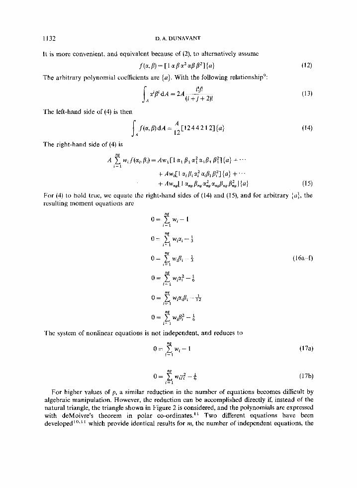
P ng nsig ssq error ifn infer time

SYMMETRICAL GAUSSIAN QUADRATURE RULES

APPENDIX I: NOTATION FOR APPENDIX I1

= Order of complete polynomial. = Number of Gaussian points and weights. = Number of significant digits. = Sum of the squares of the residuals of the moment equations. = Relative difference between exact integration and numerical quadrature. = Number of calls to subroutine func. = 1 indicates that nsig criterion of 15 was achieved. = CPU time, in seconds, required for solution of the moment equations.

1139

1140 D. A. DUNAVANT

APPENDIX I1

p= 1 ng= 1 nsig-29.0 ssq=O. error= 0. ifn= 2 infers4 time= 0 weight alpha beta gamma

1.000000000000000 0.333333333333333 0.333333333333333 0.333333333333333

p= 2 ng= 3 nsig=29.0 ssq=O. error- 8.d-29 ifn= 3 i n f e r ~ 4 time= 0 weight alpha beta gamma

0.333333333333333 0.666666666666667 0.166666666666667 0.166666666666667

p= 3 ng= 4 nsigE22.5 ssqa2.d-58 error= 2.d-28 ifn= 95 infer=l time= 0 weight alpha beta gamma

-0.562500000000000 0.333333333333333 0,333333333333333 0.333333333333333 0.520833333333333 0.600000000000000 0.200000000000000 0.200000000000000

p = 4 ng= 6 nsig=23.0 ssqm2.d-58 error= 2.d-28 ifn= 86 inferal time= 0 weight alpha beta gamma

0.223381589678011 0.108103018168070 0.445948490915965 0.445948490915965 0.109951743655322 0.816847572980459 0,091576213509771 0.091576213509771

p = 5 ng= 7 nsig=24.1 ssq=4.d-58 error- 2.d-28 ifn= 1 1 1 infer=l time= 0 weight alpha beta gamma

0.225000000000000 0.333333333333333 0.333333333333333 0.333333333333333 0.132394152788506 0.059715871789770 0.4701420641051 15 0.4701420641051 15 0.125939180544827 0.797426985353087 0.101286507323456 0.101286507323456

p= 6 ng=12 nsig=22.7 ssq=2.d-58 error= 2.d-28 ifn= 233 infer=l time= 2 weight alpha beta gamma

0.116786275726379 0.501426509658179 0.249286745170910 0.249286745170910 0.050844906370207 0.873821971016996 0.063089014491502 0.063089014491502 0.082851075618374 0.053145049844817 0.310352451033784 0.636502499121399

p= 7 ng=13 nsig=26.1 ssq=2.d-57 error= 3.d-28 ifn= 452 infer=l t i m e - 2 weight alpha beta gamma

-0,149570044467682 0.333333333333333 0.333333333333333 0.333333333333333 0.175615257433208 0.479308067841920 0.260345966079040 0.260345966079040 0.053347235608838 0.869739794195568 0.065130102902216 0.065130102902216 0.077113760890257 0.048690315425316 0.312865496004874 0.638444188569810

p= 8 ng=16 nsig=15.2 ssq=7.d-59 error= 4.d-28 ifn= 410 inferal time= 6 weight a lp ha beta gamma

0.144315607677787 0.333333333333333 0.333333333333333 0.333333333333333 0.095091634267285 0.081414823414554 0,459292588292723 0.459292588292723 0.103217370534718 0.658861384496480 0.170569307751760 0.170569307751760 0.032458497623198 0.898905543365938 0.050547228317031 0.050547228317031 0.027230314174435 0.008394777409958 0.263112829634638 0.728492392955404

p= 9 ng=19 nsig=16.3 ssq=l.d-57 error= 6.d-28 ifn= 713

0.097135796282799 0.333333333333333 0.333333333333333 0.031334700227139 0.020634961602525 0.489682519198738 0.077827541004774 0.125820817014127 0.437089591492937 0.079647738927210 0,623592928761935 0.188203535619033 0.025577675658698 0.910540973211095 0.044729513394453 0.043283539377289 0.036838412054736 0.221962989160766

weight alpha beta i nf e r=l t ime= 7

gamma 0.333333333333333 0.489682519198738 0.43708959 1492937 0.188203535619033 0.044729513394453 0.741 198598784498


p=lO ng=25 nsigu19.0 ssq~5.d-58 error- 6.d-28 ifn= 1059 infer=l time= 39 weight alpha beta gamma

0.090817990382754 0.333333333333333 0.333333333333333 0.333333333333333 0,036725957756467 0.028844733232685 0.485577633383657 0.485577633383657 0.045321059435528 0.781036849029926 0.109481575485037 0.109481575485037 0.072757916845420 0.141707219414880 0.307939838764121 0.550352941820999 0.028327242531057 0.025003534762686 0.246672560639903 0.728323904597411 0.009421666963733 0.009540815400299 0.066803251012200 0.923655933587500

p=ll ng=27 nsiga23.5 ssqP4.d-58 error= 6.d-28 ifn= 1668

0.000927006328961 -0.069222096541517 0.534611048270758 0.077149534914813 0.202061394068290 0.398969302965855 0.059322977380774 0.593380199137435 0.203309900431282 0.036184540503418 0.761298175434837 0.119350912282581 0.013659731002678 0.935270103777448 0.032364948111276 0.052337111962204 0.050178138310495 0.356620648261293 0.0207-07659639141 0.021022016536166 0.171488980304042

weight alpha beta

p=12 ng=33 nsige17.8 ssqa9.d-58 error= 1.d-27 ifn= 2439

0.025731066440455 0.023565220452390 0.488217389773805 0.043692544538038 0.120551215411079 0.439724392294460 0.062858224217885 0.457579229975768 0.271210385012116 0.034796112930709 0.744847708916828 0.127576145541586 0.006166261051559 0.957365299093579 0.021317350453210 0.040 37 155 7 7 6638 1 0.11 534 34 94534698 0.2757 1326968 55 14 0.022356773202303 0.022838332222257 0.281325580989940 0.017316231108659 0.025734050548330 0.116251915907597

weight alpha beta

pp13 ng=37 nsig=16.9 ssqi2.d-57 error weight alpha

0.052520923400802 0.333333333333333 0.011280145209330 0.009903630120591 0.031423518362454 0.062566729780852 0.047072502504194 0.170957326397447 0.047363586536355 0.541200855914337 0.031167529045794 0.771151009607340 0.007975771465074 0.950377217273082 0.036848402728732 0.094853828379579 0.017401463303822 0.018100773278807 0.015521786839045 0.022233076674090

'= 8.d-28 ifn= 3804 beta

0.333333333333333 0.495048184939705 0.468716635109574 0.414521336801277 0.229399572042831 0.114424495196330 0.02481 1391363459 0.268794997058761 0.29 17 300667 34 288 0.126357385491669

inferal time= 34 gamma

0.534611048270758 0.398969302965855 0.203309900431282 0.119350912282581 0.032364948111276 0.593201213428213 0.807489003159792

infers1 time= 74 gamma

0.488217389773805 0.439724392294460 0.271210385012116 0.127576145541586 0.021317350453210 0.608943235779788 0.695836086787803 0.85801403354407 3

infer=l time= 188 gamma

0.333333333333333 0.49504818493970s 0.468716635109574 0.414521336801277 0.229399572042831 0.114424495196330 0,024811391363459 0.636351174561660 0.690 169 159986905 0.85140953783424 1

p-14 ng=42 nsigz18.7 ssqa8.d-58 error= 7.d-28 ifn= 5612 infer=l time= 278 weight alpha beta gamma

0.021883581369429 0.022072179275643 0.488963910362179 0.488963910362179 0.032788353544125 0.164710561319092 0.417644719340454 0.417644719340454 0.051774104507292 0.453044943382323 0.273477528308839 0.273477528308839 0.042162588736993 0.645588935174913 0.177205532412543 0.177205532412543 0.014433699669777 0.876400233818255 0.061799883090873 0.061799883090873 0.004923403602400 0.961218077502598 0.019390961248701 0.019390961248701 0.024665753212564 0.057124757403648 0.172266687821356 0.770608554774996 0.038571510787061 0.092916249356972 0.336861459796345 0.570222290846683 0.014436308113534 0.014646950055654 0.298372882136258 0.686980167808088 0.005010228838501 0.001268330932872 0.118974497696957 0.879757171370171

1142 D. A. DUNAVANT

p-15 ng=48 nsigm23.8 ssq=3.d-57 error weight alpha

0.001916875642849 -0.013945833716486 0.044249027271145 0.137187291433955 0.051186548718852 0.444612710305711 0.023687735870688 0.747070217917492 0.013289775690021 0.858383228050628 0.004748916608192 0.962069659517853 0.038550072599593 0.133734161966621 0.027215814320624 0.036366677396917 0.002182077366797 -0.010174883126571 0.021505319847731 0.036843869875878 0.007673942631049 0.012459809331199

= 8.d-28 ifn= 9874 1 beta

0.506972916858243 0.43 1406354283023 0.277693644847144 0.126464891041254 0.070808385974686 0 .O 18965 17024 1073 0.261311371140087 0.388046767090269 0.285712220049916 0.215599664072284 0.103575616576386

tnfer-1 time- 634 gamma

0.506972916858243 0.43 1406 354 283023 0.277693644847144 0.126464891041254 0.07 08083859 74686 0.018965170241073 0.604954466893291 0.575586555512814 0.7 2446266 307 6655 0.747556466051838 0.8839645740924 16

pa16 ng=52 nsigml5.1 ssqa4.d-57 error= 1 .d-27 ifna21626 infer=l time= 1669 weight alpha beta gamma

0.046875697427642 0.333333333333333 0.333333333333333 0.333333333333333 0.006405878578585 0.005238916103123 0.497380541948438 0.497380541948438 0.041710296739387 0.173061122901295 0.413469438549352 0.413469438549352 0.026891484250064 0.059082801866017 0.470458599066991 0.470458599066991 0.042132522761650 0.518892500060958 0.240553749969521 0.240553749969521 0.030000266842773 0.704068411554854 0.147965794222573 0.147965794222573 0.014200098925024 0.849069624685052 0.075465187657474 0.075465187657474 0.003582462351273 0.966807194753950 0.016596402623025 0.016596402623025 0.032773147460627 0.103575692245252 0.296555596579887 0.599868711174861 0.015298306248441 0.020083411655416 0.337723063403079 0.642193524941505 0.002386244192839 -0.004341002614139 0.204748281642812 0.799592720971327 0.019084792755899 0.041941786468010 0.189358492130623 0.768699721401368 0.006850054546542 0.014317320230681 0.085283615682657 0.900399064086661

pa17 ng=61 nsiga27.8 ssqn8.d-54 error- 3.d-27 ifnu33194

0.033437199290803 0.333333333333333 0.333333333333333 0.005093415440507 0.005658918886452 0.497170540556774 0.014670864527638 0.035647354750751 0.482176322624625 0.024350878353672 0.099520061958437 0.450239969020782 0.031107550868969 0.199467521245206 0.400266239377397 0.031257111218620 0.495717464058095 0.252141267970953 0.024815654339665 0.675905990683077 0.162047004658461 O.CY14056073070557 0.848248235478508 0.075875882260746 0.003194676173779 0.968690546064356 0.015654726967822 0.008119655318993 0.010186928826919 0.334319867363658 0.026805742283163 0.135440871671036 0.292221537796944 0.018459993210822 0.054423924290583 0.319574885423190 0.008476868534328 0.012868560833637 0.190704224192292 0.018292796770025 0.067165782413524 0.180483211648746 0.006665632004165 0.014663182224828 0.080711313679564

weight alpha beta inf er=l time= 4693

gamma 0.333333333333333 0.497170540556774 0.482176322624625 0.4502399 69020782 0.400266239377397 0.252141267970953 0.162047004658461 0.075875882260746 0.015654726967822 0.655493203809423 0.572337590532020 0.626001190286228 0.796427214974071 0.752351005937729 0.904625504095608


pa18 ng=70 nsigz26.3 ssqi7.d-46 error=-2.d-23 ifna25597 infer=l time= 3460 weight alpha beta gamma

0.030809939937647 0.333333333333333 0.333333333333333 0.333333333333333 0.009072436679404 0.013310382738157 0.493344808630921 0.493344808630921 0.018761316939594 0.061578811516086 0.469210594241957 0.469210594241957 0.019441097985477 0.127437208225989 0.436261395887006 0.436281395887006 0.027753948610810 0.210307658653168 0.394846170673416 0.394846170673416 0.032256225351457 0.500410862393686 0.249794568803157 0.249794568803157 0.025074032616922 0.677135612512315 0.161432193743843 0.161432193743843 0.015271927971832 0.846803545029257 0.076598227485371 0.076598227485371 0.006793922022963 0.951495121293100 0.024252439353450 0.024252439353450 -0.002223098729920 0.913707265566071 0.043146367216965 0.043146367216965 0.006331914076406 0.008430536202420 0.358911494940944 0.632657968856636 0.027257538049138 0.131186551737188 0.294402476751957 0.574410971510855 0.017676785649465 0.050203151565675 0.325017801641814 0.624779046792512 0.018379484638070 0.066329263810916 0.184737559666046 0.748933176523037 0.008104732808192 0.011996194566236 0.218796800013321 0.769207005420443 0.007634129070725 0.014858100590125 0.101179597136408 0.883962302273467 0.000046187660794 -0.035222015287949 0.020874755282586 1.014347260005363

p=19 ng=73 nsig=21.1 ssq=5.d-58 error= 1.d-27 ifn=31956

0.032906331388919 0.333333333333333 0.333333333333333 0.010330731891272 0.020780025853987 0.489609987073006 0.022387247263016 0.090926214604215 0.454536892697893 0.030266125869468 0.197166638701138 0.401416680649431 0.030490967802198 0.488896691193805 0.255551654403098 0.024159212741641 0.645844115695741 0.177077942152130 0.016050803586801 0.779877893544096 0.110061053227952 0.008084580261784 0.888942751496321 0.055528624251840 0.002079362027485 0.974756272445543 0.012621863777229 0.003884876904981 0.003611417848412 0.395754787356943 0.025574160612022 0.134466754530780 0.307929983880436 0.008880903573338 0.014446025776115 0.264566948406520 0.016124546761731 0.046933578838178 0.358539352205951 0.002491941817491 0.002861120350567 0.157807405968595 0.018242840118951 0.223861424097916 0.075050596975911 0.010258563736199 0.034647074816760 0.142421601113383 0.003799928855302 0.010161119296278 0.065494628082938

weight alpha beta

p=20 ng=79 nsig=25.6 ssq=4.d-47 e r r o ~

0.033057055541624 0.333333333333333

0.011660052716448 0.023574084130543 0.022876936356421 0.089726636099435 0.030448982673938 0.196007481363421 0.030624891725355 0.4882 14 180481 157 0.024368057676800 0.647023488009788 0.0 15997432032024 0.79 16 582893 26483 0.007698301815602 0.893862072318140

0.001751134301193 0.976836157186356 0.016465839189576 0.048741583664839 0.00 48 3 9 0335 40485 0.00 6 3 14 1 15 9 48 605 0.025804906534650 0.134316520547348 0.008471091054441 0.013973893962392 0.018354914106280 0.075549132909764

0.010112684927462 0.026686063258714 0.003573909385950 0.010547719294141

weight alpha

0.000867019185663 -0.001900928704400

-0.000632060497488 0.916762569607942

0.000704404677908 -0.008368153208227

.=-5 .d-24 if n=49869 beta

0.333333333333333 0.500950464352200 0.488212957934729 0.455136681950283 0.401996259318289 0.255892909759421 0.176488255995106 0.104 170855336758 0.053068963840930 0.04 1618715196029 0.011581921406822 0.344855770229001 0.377843269594854 0.306635479062357 0.249419362774742 0.2 12775724802802 0.146965436053239 0.137726978828923 0.059696109149007

i nf e r= 1 t ime= 105 0 2 gamma

0.333333333333333 0.489609987073006 0.454536892697893 0.401416680649431 0.255551654403098 0.177077942152130 0.110061053227952 0.055528624251840 0.012621863777229 0.600633794794645 0.557603261588784 0.720987025817365 0.594527068955871 0.839331473680839 0.701087978926173 0.822931324069857 0.9 24 344 25 26 20 784

infer=l time=10258 gamma

0.333333333333333 0.500950464352200 0.488 2 129 579 34 7 2 9 0.455136681950283 0.40 1996259318289 0.255892909759421 0.176488255995106 0.104170855336758 0.053068963840930 0.041618715196029 0.011581921406822 0.606402646106160 0.615842614456541 0.559048000390295 0.736606743262866 0.7 11 67 5 14 22874 34 0.861402717154987 0.835586957912363 0.929756171556853

1144 D. A. DUNAVANT

APPENDIX 111

C

10 C

20 C

C

30

C

40

5 0

6 0

C

70

80 C

C

program main implicit double precision (a-h,o-z) real tl, t2 external func dimension parm(4),x(45),f(44),xjac(44,45),xjtj(lO35),

common nO,nl,n2,ilb,ile,i2b,i2e,inu(44,2),dnu(44) data p a r m / 4 * 0 . d 0 / , x / 4 5 * 0 . d O / , f ~ 4 4 * O . d O / , x j a c / l 9 8 O * O . d O / ,

+ xjtj/1035*0.dO/,work/1348*O.d0/, + w / l 9 * 0 . d 0 / , a l p h a / l 9 * O . d O / , b e t a / 1 9 * 0 , d 0 / , g a m m a / l 9 * O . d 0 /

calculate the order of the polynomial read (5,lO) ip for mat (15 ) calculate the number of groups of multiplicity 1,3 and 6 read (5,20) nO,nl,n2 format (315) calculate the sum of the number of groups nsum=nO+nl+nZ calculate the pointers for nl and n2 i 1 b=nO+l ile=ilb+2*nl-l i2b=i 1 e+l i2e=i2b+3*n2-1 calculate the number of gaussian points and weights ng=n0+3*n1+6*n2 calculate the number of unknowns n=n0+2 *n 1+3 *n2 calculate the number of equations ipcopy=ip do 30 i=1,10 if ((ipcopy-6).ge.O) ipcopy=ipcopy-6 if(ipcopy.eq.0) ialpha=3 if((ipcopy.eq.l).or.(ipcopy.eq.5)) ialpha-4 if((ipcopy.eq.2).or.(ipcopy.eq.4)) ialphat-1 if(ipcopy.eq.3) ialpha=O m=((ip+3)**2+ialpha)/12 calculate the initial approximation if (nO.eq.1) read (5,40) x(1) format(dl0.0) if(nl.ne.O) read (5,50) (x(i),i=ilb,ile) format(2dl0.0) if(n2.ne.0) read (5,60) (x(i),i=i2b,i2e) format(3dl0.0) if(n2.eq.0) go to 80 calculate the n2 angle in radians pi=4.dO*datan(l.d0) do 70 i=i2b,i2e,3 x(i+2)=x(i+2)*pi/l80.dO calculate inu and dnu ca 11 nu (ip , inu , dnu ) calculate the polar system weights and points call second(t1) call zxssq(func,m,n,l5,0.dO,O.dO,lOOOOO,O,

+ work(1348),w(19),alpha(l9),beta(l9),gamma(1~)


+

C

C

90 +

100

110

C

10 C

10 2 0

30

parm,x,s8q,f,xjac,44,xjtj,work,infer,ier) call second(t2) it ime=i n t ( t 2- t 1 ) if n=idint (work( 2)) calculate the area system weights and points call area (x,w,alpha,beta,gamma) calculate the relative error of the integral call poly (ip,nO,nl,n2,nsum,w,alpha,beta,gamma,error) write(6,go) ip,ng,work(3),ssq,error,ifn,infer,itime format(' p=',i2,' ng;',i2,' nsig=',f4.1,' ssq=',lpd7.0,

write (6,100 ) format(/7x, 'weight',l4x, 'alpha',l4x, 'beta8,15x,'gamma') write(6,llO) (w(i),alpha(i),beta(i),gamma(i),i=l,nsum) format (4f 19.15 ) stop end

' error=',lpd7.0, ifn=',i5,' infer=',il,' time=',i5)

subroutine nu(ip,inu,dnu) implicit double precision (a-h,o-z) dimension inu (44,2) ,dnu(44) calculate the ith pair (j,3k) icount=l

do 10 j=l,ippl jpl= j+l do 10 k3=1, jp1,3 if(mod(j-l+k3-1,2).eq.l) go to 10 inu(icount, l)=j-l inu(icount,Z)=k3-1 icount =icount+l c ont i nu e calculate dnu(i),i=l,44 dnu( 1)=+ 1 .dO et c dnu ( 44 ) =+ 1 .do/ 220. dO return end

ippl=ip+l

subroutine func(x,m,n,f) implicit double precision (a-h,o-z) dimension x(n) , f (m) common nO,nl,n2,ilb,ile,i2b,iZe,inu(44,2),dnu(44) do 40 im=l,m f (im)=-dnu(im) if((im.eq.l).and.(nO.eq.l)) f(l)=f(l)+x(l) if(nl.eq.O) go to 20 do 10 i=ilb,ile,2 f (im)=f (im)+x(i )*x( i+l )**inu (im, 1 ) if(n2.eq.0) go to 40 do 30 i=iZb,iZe,3 dk3=dble(float(inu(im,2))) f(im)=f(im)+x(i)*x(i+l)**inu(im,l)*dcos(dk3*x(i+Z))

1146

40

I). A. DUNAVANT

continue return end

10

20 30

4 0 5 0

C

C

1 0 20

30 40

subroutine area (x,w,alpha,beta,gamma) implicit double precision (a-h,o-z) dimension x(45),~(19),alpha(l9),beta(19),gamma(l9) common nO,nl,n2,ilb,ile,i2b,i2e,inu(44,2),dnu(44) icount=l if(nO.eq.0) go to 10 w(icount)=x( 1) alpha(icount)=l.d0/3.dO beta(icount)=alpha(icount) gamma(icount)=alpha(icount) icount=icount+l if(nl.eq.O) go to 30 do 2 0 i=ilb,ile,2 w (icount )=x( i)/3 .dO alpha(icount)=(l.d0-2.dO*x(i+l))/3.d0 beta(icount)=(l,dO-alpha(icount))/2.d0 gamma(icount)=beta(icount) icount =icount+l if(n2.eq.0) go to 50 do 40 i=i2b,i2e,3 w(icount)=x(i)/6.d0 r=x( i+l ) a=x(i+2) alpha(icount)=(l.dO-Z.dO*r*dcos(a))/3.d0 beta(icount)=(l.dO+r*dcos(a)-dsqrt(3.dO)*r*dsin(a))/3.d0 gamma(icount)=l.dO-alpha(icount)-beta(icount) i count =i count+l return end

subroutine poly (ip,n0,nl,n2,nsum,w,alpha,beta,gamma,error) implicit double precis ion (a-h, 0 - 2 ) dimension w(l9),alpha(l9),beta(l9),gamma(l9) calculate the exact integral exact=2 .dO*fac( ip)/fac( ip+2) calculate the appro xi mate i nt e g ra 1 sum=O. dO if(no.ne.0) sum=sum+w(l)*alpha(l)**ip if (nl.eq.0) go to 20 nO 1 =no+ 1 nOnl=nO+nl do 10 i=nOl,nOnl sum=sum+w(i)* (alpha( i)**ip+2 .dO*beta(i)**ip) if(n2.eq.0) go to 4 0 nOnll=nO+nl+l nOnln2=nO+nl+n2 d o 30 i=nOnll ,nOnln2 sum=sum+w(i)*2.d0*(alpha(i)**ip+beta(i)**ip+gamma(i)**ip) approx=sum


error=(exact-approx)/exact r e t u r n e n d

d o u b l e p r e c i s i o n f u n c t i o n f a c ( n ) i m p l i c i t d o u b l e p r e c i s i o n ( a - h , o - z ) f a c = l .dO i f ( n . e q . O ) r e t u r n d o 10 i = l , n

r e t u r n e n d

1 0 f a c = f a c * d b l e ( f l o a t ( i ) )

S a m p l e i n p u t f o r p = 2 0

20 1

0 . 0 1 9 0 . 0 2 1 0 . 0 4 8 0 . 0 5 1 0 . 0 7 2 0 . 0 8 0 0 . 0 6 7 0 . 0 6 1 0 . 0 3 6 0 . 0 1 9 0 . 0 0 5 0.110 0 . 0 6 8 0 . 1 3 4 0 . 0 4 1 0 . 0 9 8 0 . 0 0 5 0 . 0 5 0 0 . 0 1 5

10 8

+0.5 + 0 . 4 2 5 + O . 3 2 5 +0 .2 - 0 . 2 7 5 - 0 . 4 5 - 0 . 6 2 5 - 0 . 8 - 0 . 9 2 5 - 1 .

0 . 4 5 0 . 5 5 0 . 3 7 5 0 .7 0 . 6 0 . 8 0 . 7 2 5 0 . 9 2 5

3 0 . 3 0 . 4 0 . 4 5 . 5 0 . 5 2 . 5 5 5 . 57 .5

REFERENCES

1. P. Hillion, ‘Numerical integration on a triangle’, 1nt . j . numer. methods eng., 11, 797-815 (1977). 2. C. T. Reddy and D. J. Shippy, ‘Alternative integration formulae for triangular finite elements’, Int. j . numer. methods

3. Y. Yamada, Y. Ezawa, 1. Nishiguchi and M. Okabe, ‘Reconsiderations on singularity or crack tip elements’, Int. j .

4. R. G. Anderson, B. M. Irons and 0. C. Zienkiewicz, ‘Vibration and stability of plates using finite elements’, Int. J . Solids

5. M. Abramowitz and I. A. Stegun, Handbook ofMathematica1 Functions, 9th printing, Dover Publications, New York. 6. P. Sylvester, ‘Symmetric quadrature formulae for simplexes’, Math. Comput., 24, 95-100 (1970). 7. P. C. Hammer, 0. J. Marlowe and A. H. Stroud, ‘Numerical integration over simplexes and cones’, Math. Tahl. Natn.

8. G. R. Cowper, ‘Gaussian quadrature formulas for triangles’, Int. j . numer. methods eng., 7,405-408 (1973). 9. M. A. Eisenberg and L. E. Malvern, ‘On finite element integration in natural coordinates’, In t . j . numer. methods eng., 7,

10. M. E. Laursen and M. Gellert, ‘Some criteria for numerically integrated matrices and quadrature formulas for

1 1 . J. N. Lyness and D. Jespersen, ‘Moderate degree symmetric quadrature rules for the triangle’, J . Inst. Maths, Applics.,

eng., 17, 133-139 (1981).

numer. methods eng., 14, 1525-1544 (1979).

Struct., 1031-1055 (1968).

Rex Coun. Wash., 10, 130-137 (1956).

574-575 (1973).

triangles’, Int. j . numer. methods eng., 12, 67-76 (1978).

15, 19-32 (1975).

1148 D. A. DUNAVANT

12. J. N. Lyness, Private communication. 13. M A C S Y M A Primer, Laboratory For Computer Science, Massachusetts Institute of Technology, 1978. 14. K. L. Hiebert, ‘An evaluation ofmathematicdl software that solves systems ofnonlinear equations’, ACM Trans. Math.

15. IMSLLihrary Reference Manual, 9th edn, International Mathematical and Statistical Libraries, Houston, Texas, 1981. 16. B. Irons and S. Ahmad, Techniques nfFinite Elements, Ellis Horwood, Chichester, U.K., 1980. 17. G. M. L. Gladwell, ‘Orthogonal polynomials related to triangles’, Proc. Symp. on Computer Aided Engineering, Univ. of

18. T. Moan, ‘Experiences with orthogonal polynomials and best numerical integration formulas on a triangle, with

Sqftwure, 8, 5-20 (1982).

Waterloo, 207-214 (1971).

particular reference to finite element approximations’, ZAMM, 54, 501 -508 (1974).

Documents

High degree efficient symmetrical Gaussian quadrature