ANZJS-11-10-008 Final

EVALUATION OF RECURSIVE DETECTION METHODS

FOR TURNING POINTS IN FINANCIAL TIME SERIES

Carlo Grillenzoni

University IUAV of Venice

Summary

Timely identification of turning points in economic time series is important for plan-

ning control actions and achieving profitability. This paper compares sequential

methods for detecting peaks and troughs in stock values and deciding the time to

trade. Three semi-parametric methods are considered: double exponential smooth-

ing, time-varying parameters and prediction errors statistics. These methods are

widely used in monitoring, forecasting and control, and their common features are

recursive computation and exponential weighting of observations. The novelty of

this paper is to select smoothing and alarm coefficients on the maximization of

the gain (the difference in level between subsequent peaks and troughs) of sample

data. The methods are compared on applications to leading financial series and with

simulation experiments.

Key words: adaptive estimation; exponential smoothing; gain maximization; pre-

diction errors; time-varying parameters.

Department of Planning, University IUAV, St. Croce 1957, 30135 Venezia, Italy.

e-mail: carlog@iuav.it

Acknowledgments. I thank the reviewers for their help in improving this work.

1

1. Introduction

An important problem in the analysis of economic time series is the detection of

turning points, i.e. sequential identification of the periods where a series changes its

local slope (e.g. Zellner et al., 1991). This issue is different from forecasting, which

aims to provide pointwise predictions of future values, nevertheless it is crucial for

planning control actions. For example, in macroeconomics, knowing the beginning of

a recession leads to an increase of government expenditure or an expansion of money

supply; instead, in finance it leads to selling equities or taking short positions. These

actions were massively undertaken by agents and authorities during the financial

crisis of 2008, although timeliness of decisions was missed in many cases.

Analysis of turning points of nonstationary time series has been developed in

economics and engineering where, generally speaking, it has followed three ap-

proaches. The first one consists of smoothing series with low-pass filters; subse-

quently, first and second differences of the extracted signals are evaluated as the

order conditions of continuous functions (e.g. Canova, 2007). The second approach

arises from change-point problems and uses hypothesis testing of mean-shift in prob-

ability distributions. Typical statistics are likelihood ratio (LR) and posterior prob-

ability, which become linear under Gaussianity (see Lai, 2001 and Ergashev, 2004).

The third approach consists of monitoring variability over time of regression para-

meters, which represent the local slope of the series. Switching parameter models

consider two or more states, whereas adaptive estimators leave parameters to move

freely (e.g. Grillenzoni, 1998 or Ljung, 1999). The second approach can be inte-

grated in the framework of the third by means of prediction errors.

There are some drawbacks involved by these approaches: Smoothing methods

tend to identify turning points on the basis of trend-cycle components estimated on

the entire data-set. This feature involves problems of accuracy of end-point estimates

and timeliness of detection (e.g. Kaiser & Maravall, 2001). Change-point methods

are mostly concerned with locally stationary processes, where they monitor shifts in

the mean. Now, turning-points and change-points have a different nature, and Van-

der Wiel (1996) showed the loss of optimality that test statistics have in the presence

2

of nonstationarity. Finally, effectiveness of time-varying parameter methods can be

hindered by a-priori assumptions made on the dynamic of coefficients. This is the

case, for example, of stochastic coefficients and hidden Markov modelings which

require complex estimators, such as Kalman filter and expectation-maximization

(EM) algorithms, see Marsh (2000).

To avoid these drawbacks, this paper focuses on exponentially weighted methods

which discount past observations and can be easily implemented recursively. In

particular, we use double exponential smoothers (DES) to extract trend components

of the series; we apply exponentially weighted least squares (EWLS) to estimate

time-varying parameters (TVP); and we consider exponentially weighted moving

averages (EWMA) of prediction errors as test statistics. Apart from the common

nonparametric nature and the similar computational approach, these methods have

substantial relationships at statistical level. This will we shown in the paper by

providing a unified framework to the use of exponential methods in the sequential

detection of turning points of time series.

All aforementioned methods employ smoothing coefficients which must be ap-

propriately designed. In traditional contexts, these coefficients are selected according

to forecasting and control rules, mostly based on prediction errors. Such criteria,

however, may not be optimal in turning point detection. Moreover, monitoring

schemes involve other coefficients related to alarm limits of decision rules. This pa-

per proposes to select smoothing and alarm coefficients through the maximization

of the level difference between subsequent troughs and peaks. Since maximum dif-

ference occurs in correspondence of actual turning points, it follows that proposed

solution is consistent with unbiased detection. Further, since trading strategies

usually pursue the goal of buying low and selling high stock values, the proposed

solution corresponds to an approach of maximum gain.

The plan of the work is as follows: Section 2 provides model representation

and estimation, and decision rules for turning point detection. Section 3 deals with

selection of smoothing coefficients and alarm limits. Section 4 applies the methods

to various financial series and compares their performance.

3

2. Detection Methods for Turning Points

Stationarity of time series is usually an abstract concept, especially for eco-

nomic phenomena which continuously evolve. Real data exhibit trend components

and changes of regime which characterize evolution of first and second moments.

Modeling non-stationary time series has a long history and has been developed at

various levels. Deterministic trend models have been replaced by nonparametric

techniques which allow greater adaptivity and robustness (e.g. Grillenzoni, 2009).

Divergent processes, such as autoregressive (AR) models with characteristic roots

greater than one, were studied since 50s and now have a solid inferential framework

(see Fuller, 1996). Time-varying parameters have a more recent history and still

present challenging issues at analytical level; however, some authors have applied

them also to AR models with unit-roots (e.g. Granger & Swanson, 1997). In this

section we discuss the main approaches of modeling, and we present various methods

for detecting turning points.

2.1. Detection through smoothing methods

Given a non-stationary time series Xt, the model representation which is as-

sumed in many smoothing problems is given by

Xt = µ(t) + xt , xt ∼ f(0, σ2

t ) ; t = 1, 2 . . . T, (1)

where µ(t) is a deterministic function with possible discontinuities and xt is nearly

stationary in mean. Autocorrelation of xt does not affect the bias of nonparametric

smoothers, and only influence their variance (see Beran & Feng, 2002).

In the literature turning points tend to be defined on Xt, or its realizations (e.g.

Zellener et al., 1991); however, this approach is problematic being Xt a stochastic

process. Since µ(t) is deterministic, it enables a precise definition of turning points

as local troughs (ri) and local peaks (si) of the function itself, namely

ri : µ(ri − k) ≥ . . . ≥ µ(ri − 1) > µ(ri) < µ(ri + 1) < . . . < µ(ri + k),

si : µ(si − k) ≤ . . . ≤ µ(si − 1) < µ(si) > µ(si + 1) > . . . > µ(si + k),

4

where k is a positive integer. Given the sampling interval [1,T ], we assume that the

double sequence {ri, si} contains n < T/2 pairs, which can be ordered as

1 ≤ r1 < s1 < r2 < . . . < ri < si < . . . < sn−1 < rn < sn ≤ T. (2)

In this subsection we identify periods {ri, si} by estimating the function µ(t), with

smoothing methods, and then by identifying its local minima and maxima.

Common nonparametric methods, such as kernel regression and splines, have

a two-sided structure. These methods estimate µ(t) using both past and future

observations Xt±k. This involves difficulties to implement smoothers sequentially

and reducing their bias at end-points (see Kaiser & Maravall, 2001). On the other

hand, one-sided methods based on the Kalman filter, involve multiple smoothing

coefficients which cannot be easily selected (e.g. Harvey & Koopman, 2009).

The simplest recursive smoother is the exponential moving average. It assumes

that the series Xt fluctuates around a constant mean. An extention, suitable in

the presence of trend components, is the double exponential smoother, see Brown

(1963). Using a single coefficient λ, the algorithm is given by

mt = λ mt−1 + (1 − λ) Xt , m0 = X0,

µt = λ µt−1 + (1 − λ) mt , µ0 = m0, (3)

where λ ∈ (0, 1] gives more weight to recent observations. The first equation is the

simple smoother (EWMA), and provides the one-step-ahead forecast Xt+1 = mt.

The second equation is the double smoother (DES), and it will be used to estimate

the trend function µ(t) of the model (1).

The double smoother can also be used in multiple-step-ahead forecasting. As

in regression models, the forecast function Xt+h, h > 0 can be expressed as the sum

of a level and a slope component. In the approach of Brown (1963, p. 128), these

components can be estimated from the system (3) as follows

level at =(

2 mt − µt

)

,

slope bt =(

mt − µt

)

(1 − λ)/λ,

Xt+h = at + bt h , h = 1, 2, 3 . . . (4)

5

The last equation has time-varying parameters, hence it is not a linear model in a

strict sense (see Granger, 2008). At computational level, merging equations (3) and

(4) leads to the Holt’s algorithm, which expresses at, bt as functions of Xt

at = λ(

at−1 + bt−1

)

+ (1 − λ) Xt , a0 = X0,

bt = λ bt−1 + (1 − λ)(

at − at−1

)

, b0 = 0, (5)

see Chatfield et al. (2001) and Lawrence et al. (2009).

For the sake of parsimony, we have employed a single coefficient λ in both

equations of (3)-(5); in the next section we discuss its selection. As regards the

estimation of the model (1), one can use either µt or at, although the latter is less

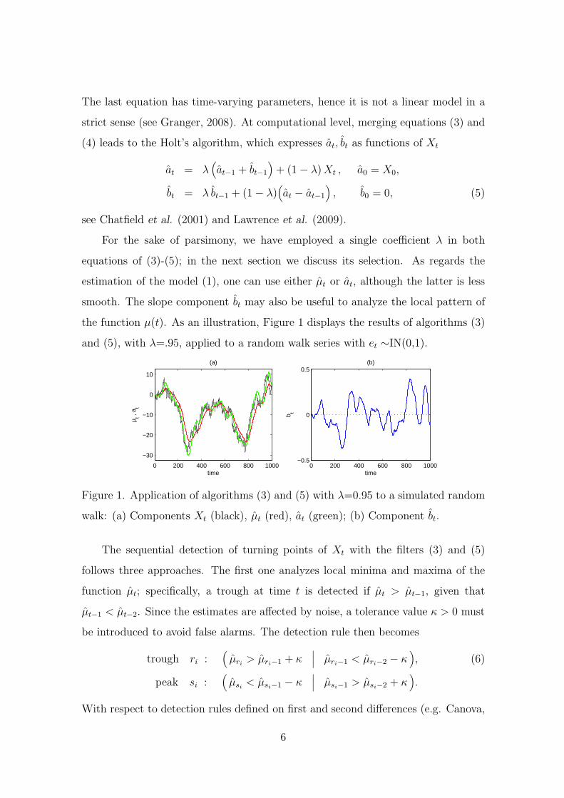
smooth. The slope component bt may also be useful to analyze the local pattern of

the function µ(t). As an illustration, Figure 1 displays the results of algorithms (3)

and (5), with λ=.95, applied to a random walk series with et ∼IN(0,1).

0 200 400 600 800 1000

−30

−20

−10

0

10

time

(a)

µ t , a t

0 200 400 600 800 1000−0.5

0

0.5

time

(b)

b t

Figure 1. Application of algorithms (3) and (5) with λ=0.95 to a simulated random

walk: (a) Components Xt (black), µt (red), at (green); (b) Component bt.

The sequential detection of turning points of Xt with the filters (3) and (5)

follows three approaches. The first one analyzes local minima and maxima of the

function µt; specifically, a trough at time t is detected if µt > µt−1, given that

µt−1 < µt−2. Since the estimates are affected by noise, a tolerance value κ > 0 must

be introduced to avoid false alarms. The detection rule then becomes

trough ri :(

µri> µri−1 + κ

∣

∣

∣ µri−1 < µri−2 − κ)

, (6)

peak si :(

µsi< µsi−1 − κ

∣

∣

∣ µsi−1 > µsi−2 + κ)

.

With respect to detection rules defined on first and second differences (e.g. Canova,

6

2007, Ch. 3), the advantage of (6) is that it points out the role of the tolerance

coefficient κ > 0, which reduces the number of wrong detections.

The second approach is inspired by the oscillation method used in technical

analysis of finance (e.g. Neely & Weller, 2003). It consists of monitoring the paths

of one-sided moving averages of different size. If a short-term average crosses the

long-term one from below, then a trough is detected, (a peak occurs in the opposite

case). Applying this principle to simple and double smoothers in (3), we have a

trough at time t if mt > µt, given that mt−1 < µt−1. Introducing a tolerance value

κ > 0 as in (6), we have the detection scheme

trough ri :(

mri> µri

+ κ∣

∣

∣ mri−1 < µri−1 + κ)

, (7)

peak si :(

msi< µsi

− κ∣

∣

∣ mri−1 > µri−1 − κ)

.

The third approach focuses on the component bt of the filter (5), which measures

the local slope of µ(t). In correspondence of turning points the sign of the slope

inverts; in particular, before a trough bt < 0, and after it bt > 0. Hence, introducing

a tolerance value κ > 0, the detection rule is given by

trough ri :(

bri> 0 + κ

∣

∣

∣ bri−1 < 0 + κ)

, (8)

peak si :(

bsi< 0 − κ

∣

∣

∣ bsi−1 > 0 − κ)

.

The schemes (6)-(8) are usually managed on-line, where incoming observations

are processed with algorithms (3)-(5). Once r1 is detected, subsequent troughs are

ignored until the peak s1 is found, and so on. At the end of the sample {Xt}Tt=1, one

has the sequence {ri, si}ni=1 which provides the number of cycles n. Each method

requires specific values of λ, κ, and in Section 3 we discuss their selection.

2.2. Detection through time-varying parameters

The second approach to turning point detection deals with regression models

and time-varying parameters. This approach has been already introduced by the

equation (4), but in this section we develop it by considering the two systems

i) Xt = αt + βt t + e1t , e1t ∼ ID(0, σ2

1) , (9)

ii) Xt = φt Xt−1 + e2t , e2t ∼ ID(0, σ2

2) , (10)

7

they are essentially a linear trend model and a first-order autoregression. The vari-

ability of parameters is motivated by nonlinear and nonstationary components which

are present in the process Xt, see Grillenzoni (1998) and Granger (2008). We assume

that the sequences {αt, βt; φt} are deterministic and bounded, and the innovations

{e1t, e2t} are independently distributed (ID).

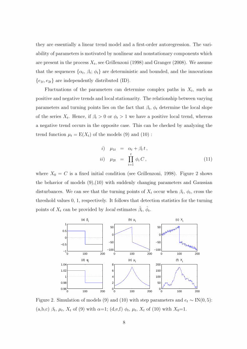
Fluctuations of the parameters can determine complex paths in Xt, such as

positive and negative trends and local stationarity. The relationship between varying

parameters and turning points lies on the fact that βt, φt determine the local slope

of the series Xt. Hence, if βt > 0 or φt > 1 we have a positive local trend, whereas

a negative trend occurs in the opposite case. This can be checked by analyzing the

trend function µt = E(Xt) of the models (9) and (10) :

i) µ1t = αt + βt t ,

ii) µ2t =t

∏

i=1

φi C , (11)

where X0 = C is a fixed initial condition (see Grillenzoni, 1998). Figure 2 shows

the behavior of models (9),(10) with suddenly changing parameters and Gaussian

disturbances. We can see that the turning points of Xt occur when βt, φt, cross the

threshold values 0, 1, respectively. It follows that detection statistics for the turning

points of Xt can be provided by local estimates βt, φt.

0 100 200−1

−0.5

0

0.5

1

(a) βt

0 100 200−100

−50

0

50

(b) µt

0 100 2000.96

0.98

1

1.02

1.04

(d) φt

0 100 2000

2

4

6

8

(e) µt

0 100 200−100

−50

0

50

(c) Xt

0 100 2000

50

100

150

200

(f) Xt

Figure 2. Simulation of models (9) and (10) with step parameters and et ∼ IN(0, 5):

(a,b,c) βt, µt, Xt of (9) with α=1; (d,e,f) φt, µt, Xt of (10) with X0=1.

8

Exponentially weighted least squares (e.g. Ljung, 1999, p. 178) is a local es-

timator which is consistent with the semiparametric nature of (9) and (10). By

defining the vectors z′t = [ 1, t ] and θ′

t = [ αt , βt ], the model (9) can be re-written

as Xt = θ′

t zt + e1t. Hence, using the coefficient 0 < λ ≤ 1, the EWLS estimator is

θt(λ) =( t

∑

i=1

λt−i zi z′

i

)−1 t∑

i=1

λt−i zi Xi , (12)

σ2

t (λ) =( t

∑

i=1

λt−i

)−1 t∑

i=1

λt−i(

Xi − θ′

i−1 zi

)2

,

where σ2t is the variance of prediction errors (see Ljung, 1999). In a similar way,

we can define the EWLS estimator of the model (10). The coefficient λ should be

inversely proportional to the rate of nonstationarity of the process Xt.

As in the discussion of Figure 2, if βt crosses the threshold 0 (or if φt crosses

the value 1), at time t = τ , then a turning point in Xt is detected at τ . Since

the estimates are affected by sampling errors, or may cross their thresholds too

frequently, tolerance limits κ > 0 should be introduced to avoid weak and false

alarms. As in the scheme (8), the detection rule for the model (9) is

trough ri :(

βri> 0 + κ

∣

∣

∣ βri−1 < 0 + κ)

, (13)

peak si :(

βsi< 0 − κ

∣

∣

∣ βsi−1 > 0 − κ)

,

analogously, for the model (10) it becomes

trough ri :(

φri> 1 + κ

∣

∣

∣ φri−1 < 1 + κ)

, (14)

peak si :(

φsi< 1 − κ

∣

∣

∣ φsi−1 > 1 − κ)

.

It is worth noting that the above strategy relies on the separate estimation of models

(9) and (10), so as to avoid interactions between βt, φt, that would keep them away

from their threshold values 0, 1.

Finally, the signaling performance of (13),(14) could be improved by smoothing

the estimates βt, φt with one-sided moving averages of few terms. Analogously, one

can reduce the volatility of φt by means of the Student statistic

Zt = (φt − 1)/√

σ2t /Rt , Rt =

t∑

j=0

λt−jX2

t−j , (15)

9

which is used in tests for unit-roots (see Fuller, 1996). Since under the null the

reference value of Zt is 0, the detection rule for (15) is similar to (13).

2.3. Detection through prediction error statistics

Detection methods based on control statistics arise from change-point problems,

where a sequence Xt is subject to a shift δ in the mean µ at an unknown time τ

(e.g. Lai, 2001). Typical detection approach consists of monitoring test statistics

sensitive to mean shifts, such as the likelihood ratio. This test requires knowledge of

the distribution f(Xt), before and after the change point τ . Under the assumption

of Gaussianity, LR statistics become linear functions of the observations. A serious

problem is the auto-correlation of series, which proportionally reduces the power of

the tests (e.g. Mei, 2006). Typical remedy is to fit Xt with a dynamical model and

then monitoring its residuals. This coincides with adaptive control techniques used

in industrial manufacturing, see Vander Viel (1996) and Box et al. (2009).

Following this approach, we model the series by combining equations (9) and

(10), so as to have independent disturbances

Xt = αt + βt t + φt Xt−1 + et , et ∼ ID(0, σ2

t ),

in general et is heteroskedastic, with 0 < σ2t < ∞. By properly choosing the entries

of the vector zt in (12), the estimator of the joint model is given by EWLS. In

recursive form (see Ljung, 1999, p. 305), it becomes

z′t = [ 1, t, Xt−1 ] ,

et = Xt − θ′

t−1zt ,

Rt = λRt−1 + zt z′

t ,

θt = θt−1 + R−1

t zt et , (16)

σ2

t = λ σ2

t−1 + (1 − λ) e2

t ,

where et are one-step-ahead prediction errors and Rt is the sum of squared regres-

sors. Apart from the initial values θ0,R0, σ20, which are asymptotically negligible

when λ < 1, the algorithm (16) is equivalent to (12).

10

0 10 200

5

10(a) trough

0 10 200

5

10(b) peak

+et

−et

Figure 3. Relationship between turning points and prediction errors.

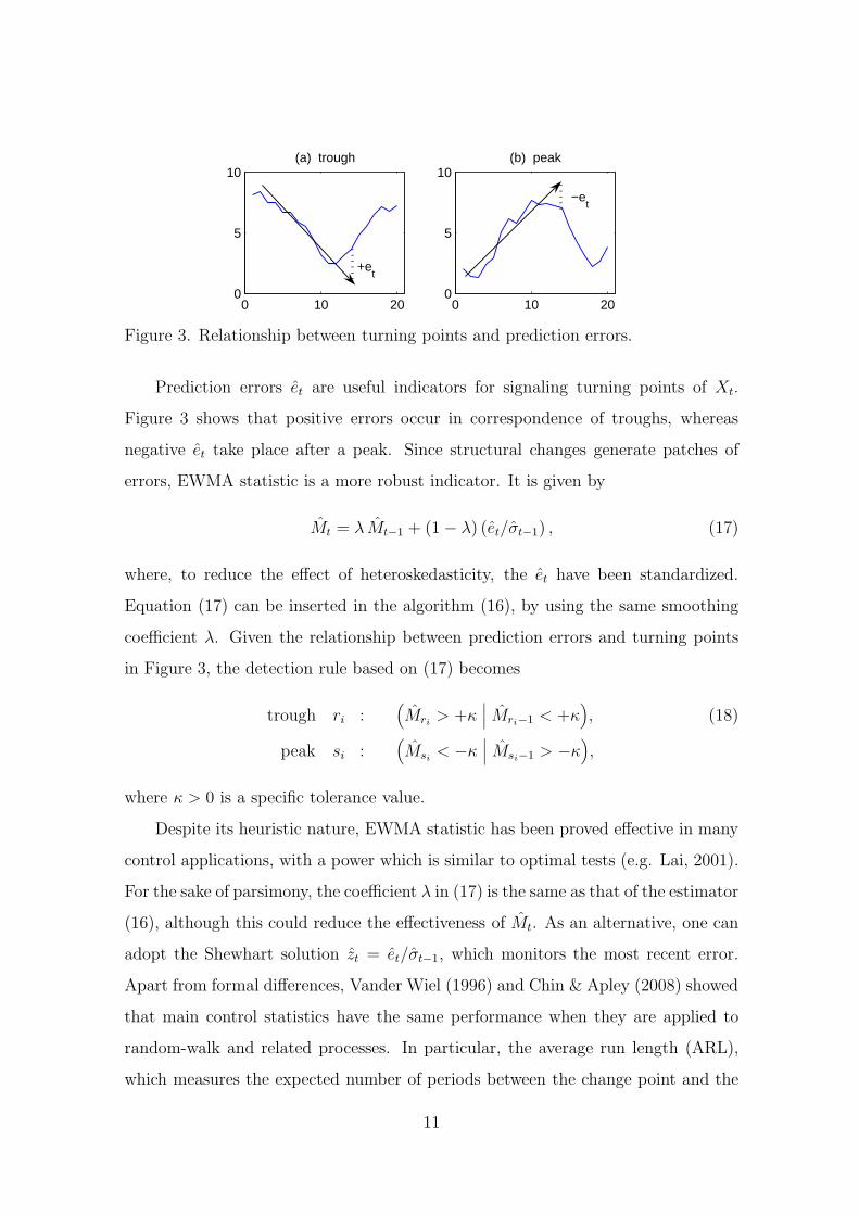
Prediction errors et are useful indicators for signaling turning points of Xt.

Figure 3 shows that positive errors occur in correspondence of troughs, whereas

negative et take place after a peak. Since structural changes generate patches of

errors, EWMA statistic is a more robust indicator. It is given by

Mt = λ Mt−1 + (1 − λ) (et/σt−1) , (17)

where, to reduce the effect of heteroskedasticity, the et have been standardized.

Equation (17) can be inserted in the algorithm (16), by using the same smoothing

coefficient λ. Given the relationship between prediction errors and turning points

in Figure 3, the detection rule based on (17) becomes

trough ri :(

Mri> +κ

∣

∣

∣ Mri−1 < +κ)

, (18)

peak si :(

Msi< −κ

∣

∣

∣ Msi−1 > −κ)

,

where κ > 0 is a specific tolerance value.

Despite its heuristic nature, EWMA statistic has been proved effective in many

control applications, with a power which is similar to optimal tests (e.g. Lai, 2001).

For the sake of parsimony, the coefficient λ in (17) is the same as that of the estimator

(16), although this could reduce the effectiveness of Mt. As an alternative, one can

adopt the Shewhart solution zt = et/σt−1, which monitors the most recent error.

Apart from formal differences, Vander Wiel (1996) and Chin & Apley (2008) showed

that main control statistics have the same performance when they are applied to

random-walk and related processes. In particular, the average run length (ARL),

which measures the expected number of periods between the change point and the

11

first alarm signal: E( τ − τ | δ ), is similar for Shewhart, CUSUM, EWMA, and LR

methods, for any δ > 0. Since financial time series are often random walk, it follows

that also the Shewhart method can detect turning points.

3. Selection of Smoothing and Alarm Coefficients

In the previous section we have presented various methods of turning point

detection. Their statistics and decision rules contain unknown coefficients that must

be properly selected. In their original context, the selection follows operative goals,

such as prediction and control. For example, in the exponential smoother (4) and in

the adaptive estimator (12), the rate λ has to optimize the forecasting performance.

In the control statistics, the shift δ is selected on the basis of the normal wandering

of the process and the limit κ has to attain the desired ARL level. It is difficult,

however, to extend this approach to the limit κ of the decision rules (6),(13),(18),

because the path of the function µt and of its turning points are complex and

unknown. In the following, we present a data-driven method for the joint selection

of λ and κ which pursues the gain maximization in a trading activity.

3.1 Maximum Gain Selection

As in the definition (2), we assume that the trend function µ(t) has n pairs of

troughs and peaks in the sampling interval [1, T ]

µ(ri) < µ(si), ri < si , i = 1, 2 . . . n < T/2 . (19)

We also assume that realizations of Xt have turning points which are close to { ri, si}.

This means that the variance of the innovation process is small compared to that of

Xt. We now define the total gain on the interval [1, T ] as the sum of the differences

in level of Xt between subsequent peaks and troughs, that is

GT (r, s) =n

∑

i=1

(

Xsi− Xri

)

, n < T/2. (20)

where r′ = [ r1, r2, . . . rn ] and s′ = [ s1, s2, . . . sn ] are the vectors of turning points.

By definition, E(GT )=∑

i[ µ(si) − µ(ri)] is maximum on [0, T ].

12

Let ri, si be the points detected with the statistics mt, µt, bt; βt, φt, Zt; et, Mt

and the decision rules (6)-(8), (13)-(15), (18). It follows that ri, si depend on the

coefficients λ, κ of detection methods. Thus, putting ri(λ, κ), si(λ, κ) within GT (·)

in (20), one can select the coefficients by maximizing the total gain:

(λ, κ) = arg maxλ,κ

GT

[

r(λ, κ), s(λ, κ)]

. (21)

where r(λ, κ) = [ r1(λ, κ), r2(λ, κ), . . . ]′, etc.. In finance, this optimizes the strategy

of buy low and sell high, which is pursued by agents. The important fact is that (21)

allows timely, hence unbiased, detection of turning points. Indeed, the maximization

of E(GT ) is equivalent to the minimization of E[∑

i(| ri − ri| + | si − si|)].

Sometimes (21) yields an excessive number of turning points, in the sense of a

value of n much greater than that expected from the visual analysis of the series. In

this case, it may be preferable to maximize the mean value GT /n, or the penalized

objective function

PT (λ, κ) =[

GT (λ, κ) − γ n]

, 0 ≤ γ < ∞ , (22)

where γ is a scale factor which allows to reach the expected number of peaks. This

approach is similar to spline smoothing, where γ provides a compromise between

fitting and smoothness.

3.2. Computational aspects

The objective functions GT and PT are usually non-smooth and may have several

local maxima. It is possible to identify the global optimum by exploring their surface

on a grid of values λi , κj ; subsequently, numerical optimization is used to improve

the solution. The search interval for λ is typically given by [.9, 1); lower values may

involve a large number of detections and may not be reliable out-of-sample.

For testing purposes, the available data-set is split into two segments T=T1 +

T2, where T1 is the in-sample (or training) period and T2 is the out-of-sample (or

evaluation) period. We carry out the selection (21) only on the T1 observations;

next we compute the measure GT2on the remaining T2 data. With this approach,

13

we are interested to check both reliability of the methods and stability over time of

estimates λ, κ. In the first period we set r1=1, and subsequent troughs are ignored

until the first peak s1 is detected; at the end, it must be sn ≤ T1.

All algorithms (3),(16),(17) are recursive and require initial values to start;

these values strongly influence the performance of the methods at the beginning.

We solve the initialization problem by assigning to m0, µ0; θ0,R0, σ20; M0 tentative

values, and then by adjusting them on ”artificial” data. Specifically, we add at the

beginning of the series, a sub-sample of size N < T1, just rescaled to the level of the

first observation, namely

X∗

−j = XN−j −(

XN − X1

)

, j = 1, 2 . . .N < T1 ,

The value of N is not very important for (3), but for (16) it should be large enough

and could also be selected with the criterion (21).

Algorithm. Summarizing the detection strategy we have the following steps:

1) Define periods T1, T2 and a grid of values λi, κj ,

2) Run recursive filters for µt, βt, et with the selected λi,

3) Apply the detection rules (6),(13),(18) with the selected κj ,

4) Collect and order the sequence of turning points {rl, sl},

5) Plot the function GT1(λi, κj) and find its maximum (λ0, κ0),

6) Improve the values of λ0, κ0 with numerical algorithms,

7) Evaluate the out-of-sample performance with GT2(λ0, κ0).

4. Application to Real and Simulated Data

In this section we apply the methods described in the previous sections to em-

pirical data and we compare their results. The exercise also serves to check the

effectiveness of the methods in trading activity. Real data are daily stock values col-

lected during the period from 1999 to 2011. We have four data-sets, which consist

of aggregate indexes and individual companies. These data were downloaded from

http://finance.yahoo.com. Finally, we perform a simulation experiment.

14

4.1. Standard and Poor’s index

Standard and Poor’s (S&P) index of New York Stock Exchange is the leading

indicator of many world stock price series. We consider the daily S&P500 in the

period Jan 4, 1999 - Sep 2, 2011, for a total of T=3189 observations. The series

is displayed in Figure 6a. Since the average number of data per year is about 251,

dates on the abscissa of the graph can be easily reconstructed. Training (in-sample)

period is defined as T1=1500, which corresponds to Dec 20, 2004. One of the issues

to be checked is whether the peak of Sep 2007 could be timely identified or at least,

the stock crash of Sep 2008 early avoided.

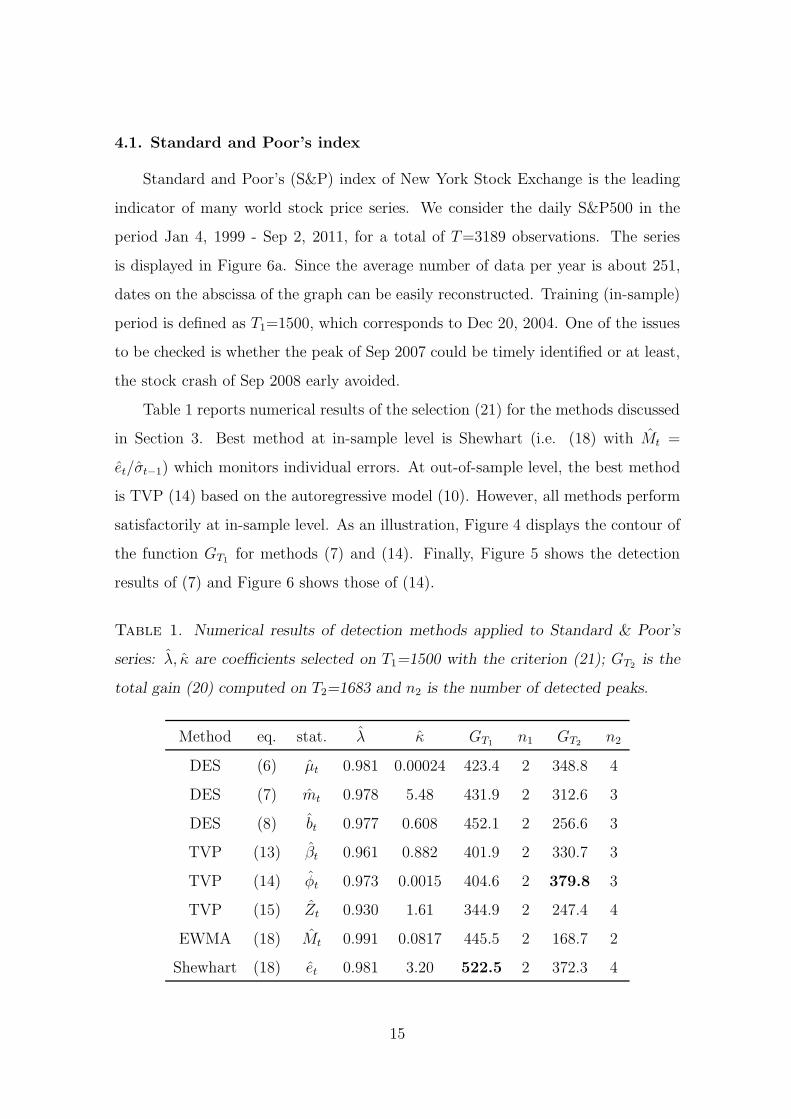
Table 1 reports numerical results of the selection (21) for the methods discussed

in Section 3. Best method at in-sample level is Shewhart (i.e. (18) with Mt =

et/σt−1) which monitors individual errors. At out-of-sample level, the best method

is TVP (14) based on the autoregressive model (10). However, all methods perform

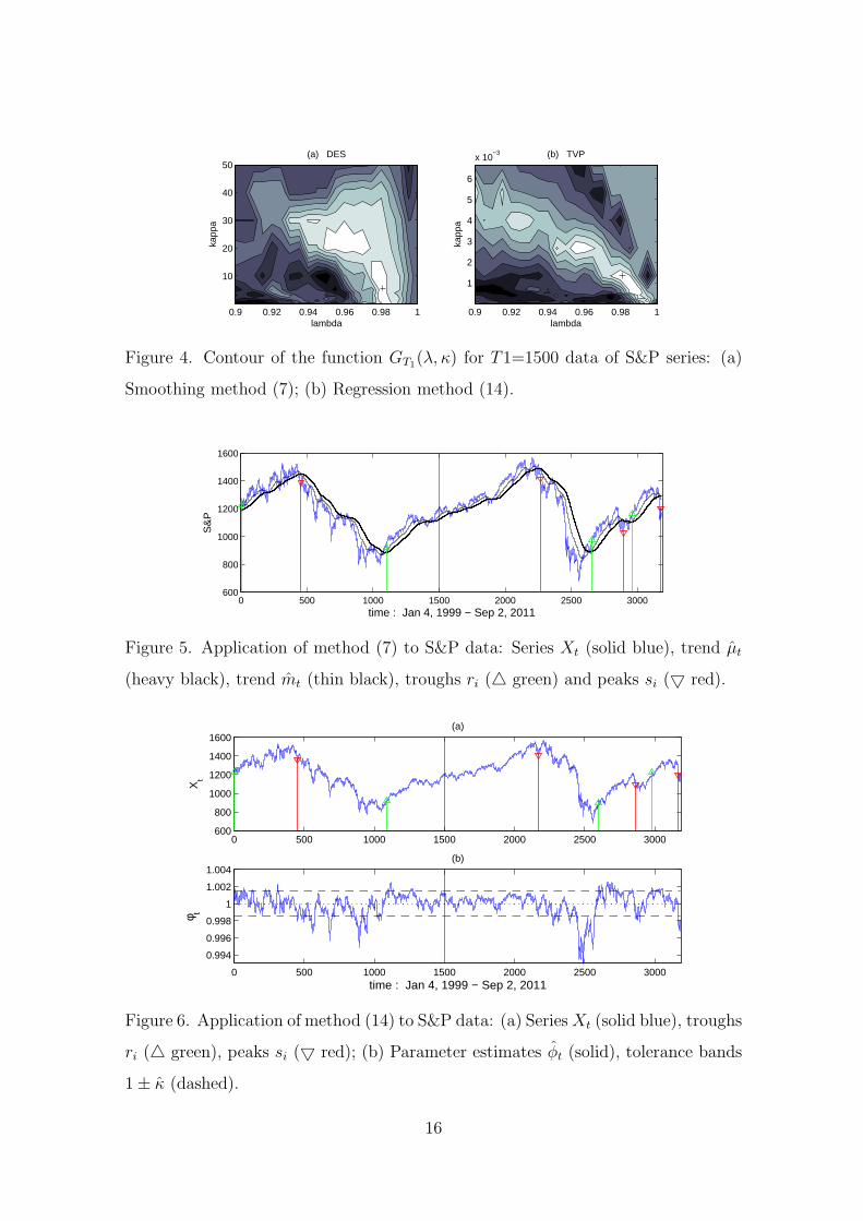
satisfactorily at in-sample level. As an illustration, Figure 4 displays the contour of

the function GT1for methods (7) and (14). Finally, Figure 5 shows the detection

results of (7) and Figure 6 shows those of (14).

Table 1. Numerical results of detection methods applied to Standard & Poor’s

series: λ, κ are coefficients selected on T1=1500 with the criterion (21); GT2is the

total gain (20) computed on T2=1683 and n2 is the number of detected peaks.

Method eq. stat. λ κ GT1n1 GT2

n2

DES (6) µt 0.981 0.00024 423.4 2 348.8 4

DES (7) mt 0.978 5.48 431.9 2 312.6 3

DES (8) bt 0.977 0.608 452.1 2 256.6 3

TVP (13) βt 0.961 0.882 401.9 2 330.7 3

TVP (14) φt 0.973 0.0015 404.6 2 379.8 3

TVP (15) Zt 0.930 1.61 344.9 2 247.4 4

EWMA (18) Mt 0.991 0.0817 445.5 2 168.7 2

Shewhart (18) et 0.981 3.20 522.5 2 372.3 4

15

lambda

kapp

a

(a) DES

0.9 0.92 0.94 0.96 0.98 1

10

20

30

40

50(b) TVP

lambda

kapp

a

0.9 0.92 0.94 0.96 0.98 1

1

2

3

4

5

6

x 10−3

Figure 4. Contour of the function GT1(λ, κ) for T1=1500 data of S&P series: (a)

Smoothing method (7); (b) Regression method (14).

0 500 1000 1500 2000 2500 3000600

800

1000

1200

1400

1600

time : Jan 4, 1999 − Sep 2, 2011

S&

P

Figure 5. Application of method (7) to S&P data: Series Xt (solid blue), trend µt

(heavy black), trend mt (thin black), troughs ri (△ green) and peaks si (▽ red).

0 500 1000 1500 2000 2500 3000600

800

1000

1200

1400

1600(a)

Xt

0 500 1000 1500 2000 2500 3000

0.994

0.996

0.998

1

1.002

1.004(b)

time : Jan 4, 1999 − Sep 2, 2011

φ t

Figure 6. Application of method (14) to S&P data: (a) Series Xt (solid blue), troughs

ri (△ green), peaks si (▽ red); (b) Parameter estimates φt (solid), tolerance bands

1 ± κ (dashed).

16

The main difference of the methods in Table 1 is at the out-of-sample level.

The disappointing performance of EWMA can be improved by exchanging λ with

(1−λ) in the statistic (17). Indeed, since λ ≈ 1 that exchange would make EWMA

similar to Shewhart method. This remark sheds light on the meaning of equation

(17) in the context of the algorithm (16). In general, all methods enable to avoid

the crash of 2008, and also signal the subsequent restarting (see Figures 5 and 6).

Given the length of the out-of-sample period, this proves reliability and stability of

the entire methodology. The performance on the after-crash period can be improved

by selecting the coefficients λ, κ using the data up to 2008 (i.e. T1=2500).

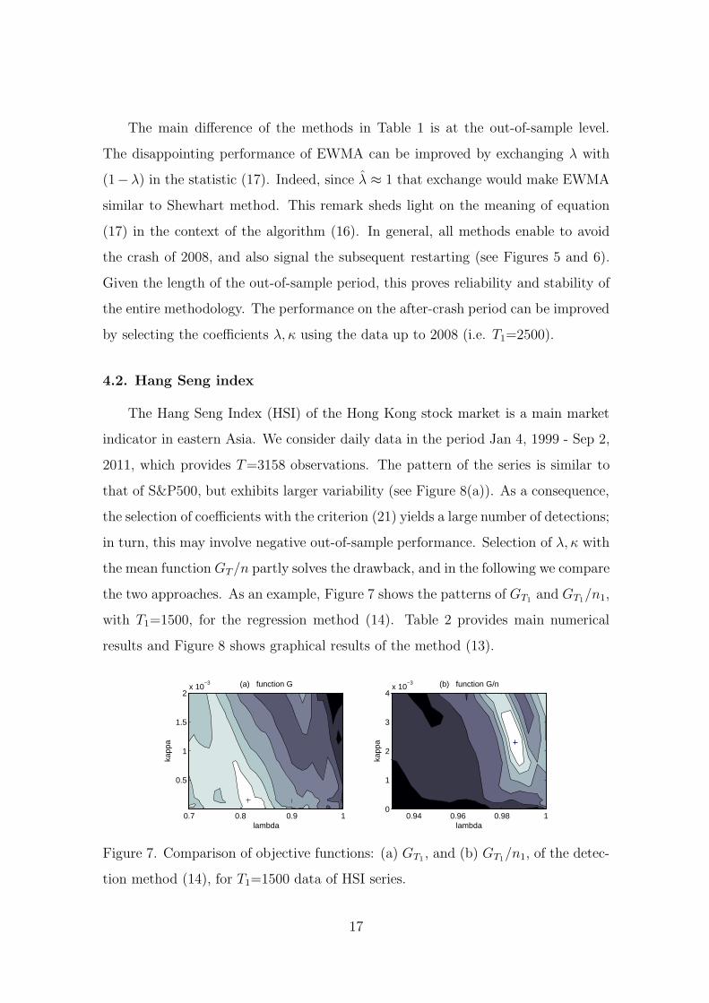
4.2. Hang Seng index

The Hang Seng Index (HSI) of the Hong Kong stock market is a main market

indicator in eastern Asia. We consider daily data in the period Jan 4, 1999 - Sep 2,

2011, which provides T=3158 observations. The pattern of the series is similar to

that of S&P500, but exhibits larger variability (see Figure 8(a)). As a consequence,

the selection of coefficients with the criterion (21) yields a large number of detections;

in turn, this may involve negative out-of-sample performance. Selection of λ, κ with

the mean function GT /n partly solves the drawback, and in the following we compare

the two approaches. As an example, Figure 7 shows the patterns of GT1and GT1

/n1,

with T1=1500, for the regression method (14). Table 2 provides main numerical

results and Figure 8 shows graphical results of the method (13).

(a) function G

lambda

kapp

a

0.7 0.8 0.9 1

0.5

1

1.5

2x 10

−3 (b) function G/n

lambda

kapp

a

0.94 0.96 0.98 10

1

2

3

4x 10

−3

Figure 7. Comparison of objective functions: (a) GT1, and (b) GT1

/n1, of the detec-

tion method (14), for T1=1500 data of HSI series.

17

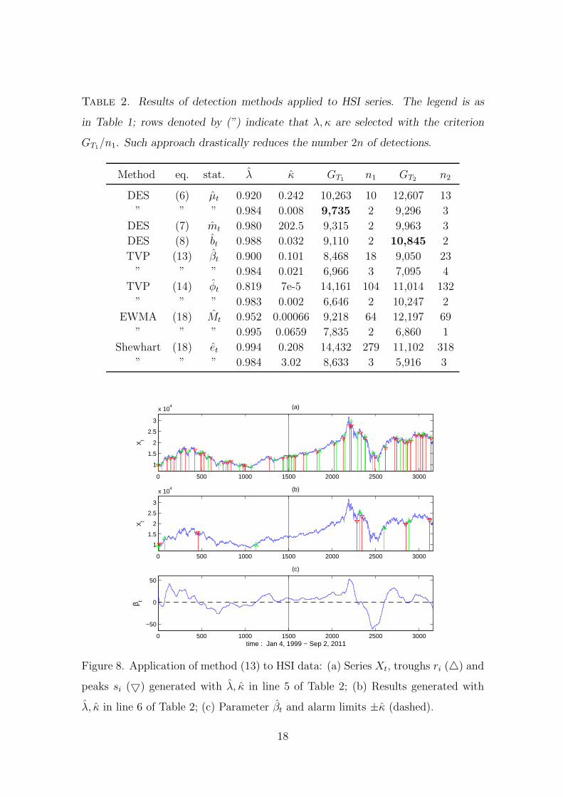
Table 2. Results of detection methods applied to HSI series. The legend is as

in Table 1; rows denoted by (”) indicate that λ, κ are selected with the criterion

GT1/n1. Such approach drastically reduces the number 2n of detections.

Method eq. stat. λ κ GT1n1 GT2

n2

DES (6) µt 0.920 0.242 10,263 10 12,607 13

” ” ” 0.984 0.008 9,735 2 9,296 3

DES (7) mt 0.980 202.5 9,315 2 9,963 3

DES (8) bt 0.988 0.032 9,110 2 10,845 2

TVP (13) βt 0.900 0.101 8,468 18 9,050 23

” ” ” 0.984 0.021 6,966 3 7,095 4

TVP (14) φt 0.819 7e-5 14,161 104 11,014 132

” ” ” 0.983 0.002 6,646 2 10,247 2

EWMA (18) Mt 0.952 0.00066 9,218 64 12,197 69

” ” ” 0.995 0.0659 7,835 2 6,860 1

Shewhart (18) et 0.994 0.208 14,432 279 11,102 318

” ” ” 0.984 3.02 8,633 3 5,916 3

0 500 1000 1500 2000 2500 3000

1

1.5

2

2.5

3

x 104 (a)

Xt

0 500 1000 1500 2000 2500 3000

1

1.5

2

2.5

3

x 104 (b)

Xt

0 500 1000 1500 2000 2500 3000

−50

0

50

(c)

time : Jan 4, 1999 − Sep 2, 2011

β t

Figure 8. Application of method (13) to HSI data: (a) Series Xt, troughs ri (△) and

peaks si (▽) generated with λ, κ in line 5 of Table 2; (b) Results generated with

λ, κ in line 6 of Table 2; (c) Parameter βt and alarm limits ±κ (dashed).

18

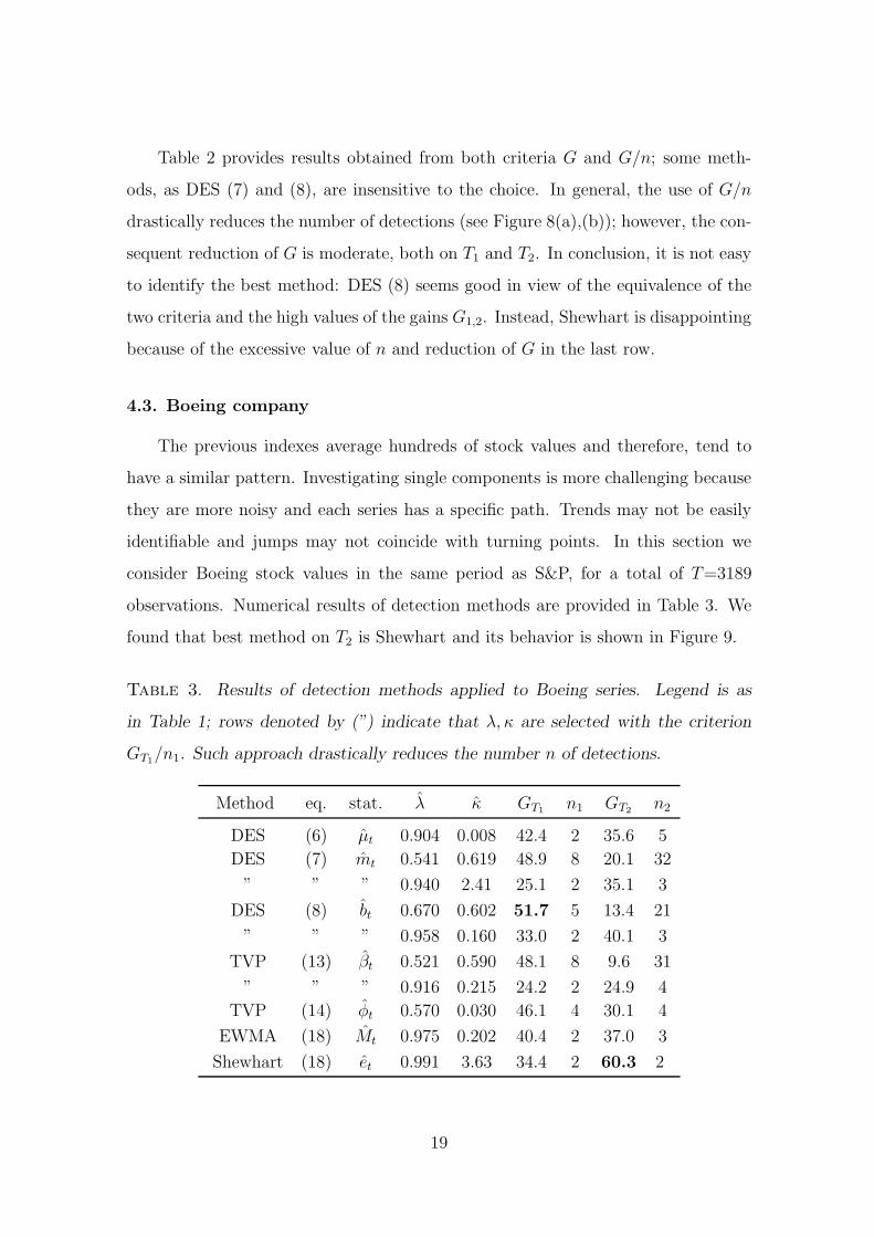
Table 2 provides results obtained from both criteria G and G/n; some meth-

ods, as DES (7) and (8), are insensitive to the choice. In general, the use of G/n

drastically reduces the number of detections (see Figure 8(a),(b)); however, the con-

sequent reduction of G is moderate, both on T1 and T2. In conclusion, it is not easy

to identify the best method: DES (8) seems good in view of the equivalence of the

two criteria and the high values of the gains G1,2. Instead, Shewhart is disappointing

because of the excessive value of n and reduction of G in the last row.

4.3. Boeing company

The previous indexes average hundreds of stock values and therefore, tend to

have a similar pattern. Investigating single components is more challenging because

they are more noisy and each series has a specific path. Trends may not be easily

identifiable and jumps may not coincide with turning points. In this section we

consider Boeing stock values in the same period as S&P, for a total of T=3189

observations. Numerical results of detection methods are provided in Table 3. We

found that best method on T2 is Shewhart and its behavior is shown in Figure 9.

Table 3. Results of detection methods applied to Boeing series. Legend is as

in Table 1; rows denoted by (”) indicate that λ, κ are selected with the criterion

GT1/n1. Such approach drastically reduces the number n of detections.

Method eq. stat. λ κ GT1n1 GT2

n2

DES (6) µt 0.904 0.008 42.4 2 35.6 5

DES (7) mt 0.541 0.619 48.9 8 20.1 32

” ” ” 0.940 2.41 25.1 2 35.1 3

DES (8) bt 0.670 0.602 51.7 5 13.4 21

” ” ” 0.958 0.160 33.0 2 40.1 3

TVP (13) βt 0.521 0.590 48.1 8 9.6 31

” ” ” 0.916 0.215 24.2 2 24.9 4

TVP (14) φt 0.570 0.030 46.1 4 30.1 4

EWMA (18) Mt 0.975 0.202 40.4 2 37.0 3

Shewhart (18) et 0.991 3.63 34.4 2 60.3 2

19

0 500 1000 1500 2000 2500 300020

40

60

80

100(a)

Xt

0 500 1000 1500 2000 2500 3000

−5

0

5

e t/σt

(b)

time : Jan 4, 1999 − Sep 2, 2011

Figure 9. Application of Shewhart method to Boeing data: (a) Series Xt, troughs

ri (△) and peaks si (▽); (b) Statistics et/σt−1 and alarm limits ±κ (dashed).

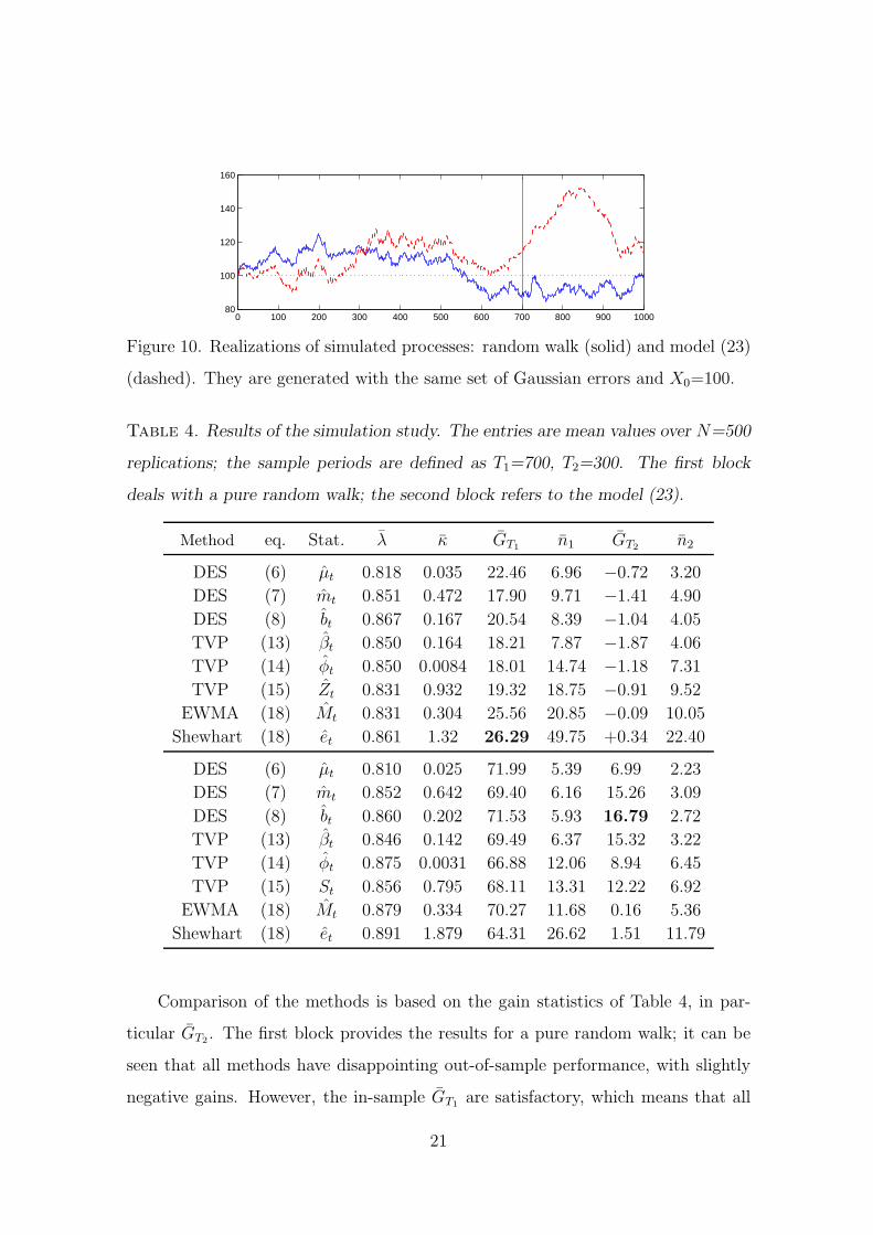
4.5. Simulation study

To evaluate in depth the methods discussed so far, it is necessary to perform

simulations experiments. Owing to the long-run behavior of stock values, the basic

model is the random walk; however, we also simulate the process under more general

non-stationarity conditions. In particular, we also consider the TVP system

Xt = φt Xt−1 + σt et , et ∼ IN(0, 1), (23)

φt = 1 + Ut , Ut = Ut−1 + ut , ut ∼ IN(0, 1),

σt = 1 + Vt , Vt = Vt−1 + vt , vt ∼ IN(0, 1),

where the realizations of parameters are rescaled to the intervals φt ∈[0.985, 1.015]

and σt ∈[0.25, 1.75]. These bounds are necessary to avoid explosiveness of Xt and

to allow positive standard deviations. Sample realizations of the processes are given

in Figure 10; it can be seen that time-varying parameters produce a volatility which

is similar to that of real financial series.

Experimental conditions are designed as follows: N=500 replications of size

T=1000 are generated for a random walk and the process (23) (see Figure 10).

They are obtained with the same set (500×1000) of Gaussian innovations et. Detec-

tion methods are trained on the period T1=700, and are evaluated on the segment

T2=300; mean values of the estimates (21) are reported in Table 4.

20

0 100 200 300 400 500 600 700 800 900 100080

100

120

140

160

Figure 10. Realizations of simulated processes: random walk (solid) and model (23)

(dashed). They are generated with the same set of Gaussian errors and X0=100.

Table 4. Results of the simulation study. The entries are mean values over N=500

replications; the sample periods are defined as T1=700, T2=300. The first block

deals with a pure random walk; the second block refers to the model (23).

Method eq. Stat. λ κ GT1n1 GT2

n2

DES (6) µt 0.818 0.035 22.46 6.96 −0.72 3.20

DES (7) mt 0.851 0.472 17.90 9.71 −1.41 4.90

DES (8) bt 0.867 0.167 20.54 8.39 −1.04 4.05

TVP (13) βt 0.850 0.164 18.21 7.87 −1.87 4.06

TVP (14) φt 0.850 0.0084 18.01 14.74 −1.18 7.31

TVP (15) Zt 0.831 0.932 19.32 18.75 −0.91 9.52

EWMA (18) Mt 0.831 0.304 25.56 20.85 −0.09 10.05

Shewhart (18) et 0.861 1.32 26.29 49.75 +0.34 22.40

DES (6) µt 0.810 0.025 71.99 5.39 6.99 2.23

DES (7) mt 0.852 0.642 69.40 6.16 15.26 3.09

DES (8) bt 0.860 0.202 71.53 5.93 16.79 2.72

TVP (13) βt 0.846 0.142 69.49 6.37 15.32 3.22

TVP (14) φt 0.875 0.0031 66.88 12.06 8.94 6.45

TVP (15) St 0.856 0.795 68.11 13.31 12.22 6.92

EWMA (18) Mt 0.879 0.334 70.27 11.68 0.16 5.36

Shewhart (18) et 0.891 1.879 64.31 26.62 1.51 11.79

Comparison of the methods is based on the gain statistics of Table 4, in par-

ticular GT2. The first block provides the results for a pure random walk; it can be

seen that all methods have disappointing out-of-sample performance, with slightly

negative gains. However, the in-sample GT1are satisfactory, which means that all

21

methods can be used in the one-step-ahead horizon. The performances on T2 signif-

icantly improve when the data are generated with the system (23). Worst methods

are those based on the prediction errors (i.e. Shewhart and EWMA); this is due

to the fact that significant errors are not sufficient conditions for the existence of

turning points. Indeed, anomalous et could even be generated by outliers and het-

eroskedasticity in the innovations. As an empirical evidence, one can see that the

low value of GT2of Shewhart is accompanied by the highest value of n2. Best meth-

ods are those based on the slope parameters bt, βt, which also have small values of

n2. Finally, even the oscillator scheme (7) performs well.

The weakness of simulation experiments is that the true model of real time

series is not known. In particular, the parametric form and the kind of non-linearity,

non-stationarity and heteroskedasticity are unknown. As we have seen in previous

applications, the detection methods have very different performances, and just one

prevails on the others. This leads to not exclude any method a-priori.

5. Discussion

In this paper we have discussed three classes of detection methods for turning

points of time series based on exponential weighting of observations. We have applied

these methods to real stock values and simulated series. A suitable evaluation can

be based on out-of-sample statistics n2 and GT2, which are the number of detected

peaks and the difference in height between subsequent troughs and peaks. The

target value for n2 is the number of peaks observable in the period T2. However,

in financial time series, definition and count of turning points may be difficult (see

e.g. Figure 8(a)). Instead, the statistic GT2is a more objective indicator because

it deals with the location of turning points and therefore, with unbiasedness of the

methods. The mean value GT2/n2 is not suitable, because it may be high also for

small values of G and n.

Analysis of statistics GT2of Tables 1-4 does not enable to conclude which method

is best overall. This means that each time series requires its specific framework.

22

Prediction errors methods (Shewhart and EWMA) are good, but tend to yield a large

value of n1 and may be unreliable out-of-sample. However, their performance could

be improved by modifying the structure of the underlying model, e.g. by including

further components, as γt Xt−2. An important role in their performance is played by

the adaptive estimator (16); especially for the treatment of heteroskedasticity with

et/σt−1. Hence, in our approach, control statistics are substantially related to TVP

methods, which do not exhibit a bad performance.

The idea of ”combining” detections provided by different methods is interesting

but problematic, because it deals with paired point processes. The various sequences

{ri, si}j (where j is the index of the methods) can be pooled together and subse-

quently ordered. While this increases the number n, it does not necessarily improve

the value of GT . Only methods with good in-sample gains should be considered.

Instead of pooling their points, one can use the various solutions in parallel, i.e. take

a decision only if it is signaled by at least two methods. This approach generally

reduces the number of detected points and so the gains.

The crucial phase in the proposed methodology is the selection of smoothing

and alarm coefficients λ and κ. It is carried out by maximizing the function GT1

on the training period T1. An important aspect to evaluate in further research is

stability over time of the selected coefficients, which determines their performance

on the period T2. In situations of strong nonstationarity and sudden changes −such

as those induced by market crashes and institutional acts− the coefficients should

be continously updated as new data become available. At the same time, oldest

observations should be discarded from the sample, so that optimal selection of the

in-sample size T1 should be investigated.

References

Beran, J. & Feng, Y. (2002). Local polynomial fitting with long-memory, short

memory and antipersistent errors. Ann. Inst. Statist. Math. 54, 291-311.

Bock, D., Andersson, E. & Frisen, M. (2008). The relation between statis-

23

tical surveillance and technical analysis in finance. In Financial Surveillance,

ed. Frisen, M. New York: Wiley, pp. 69-92.

Box, G.E.P., Luceno, A. & Del Carmen Paniagua-Quinones, M. (2009).

Statistical Control by Monitoring and Adjustment, 2nd edn. New York: Wiley.

Brown, R.G. (1963). Smoothing, Forecasting and Prediction of Discrete Time

Series. Englewood Cliffs, NJ: Prentice-Hall.

Canova, F. (2007). Methods for Applied Macroeconomic Research. Princeton,

NJ: Princeton University Press.

Chatfield, C., Koehler, B., Ord, K. & Snyder, D. (2001). A new look at

models for exponential smoothing. The Statistician 50, 147-159.

Chin, C.H. & Apley, D.W. (2008). Performance and robustness of control

charting methods for autocorrelated data. J. Korean Inst. Indus. Engin. 34,

122-139.

Ergashev, B.A. (2004). Sequential detection of US business cycle turning points:

Performances of Shiryayev-Roberts, CUSUM and EWMA procedures. Econ-

WPA n.0402001.

Fuller, W.A. (1996). Introduction to Statistical Times Series. New York: Wiley.

Granger, C.W.J. (2008). Non-linear models: where do we go next − time

varying parameter models ?. Studies Nonlin. Dynam. & Econom. 12, 1-9.

Granger, C.W.J. & Swanson, N.R. (1997). An introduction to stochastic

unit-root processes. J. Econometrics 80, 3562.

Grillenzoni, C. (1998). Forecasting unstable and nonstationary time series. Int.

J. Forecasting, 14 469-482.

Grillenzoni, C. (2009). Robust non-parametric smoothing of non-stationary

time series. J. Statist. Comput. Simul. 79, 379-393.

24

Harvey, A.C. & Koopman, S.J. (2009). Unobserved components models in

economics and finance. IEEE Contr. Syst. Magaz. 8, 71-81.

Kaiser, R. & Maravall, A. (2001). Measuring business cycles in economic

time series. Lecture Notes in Statistics 154, New York: Springer Verlag.

Lai, T.L. (2001). Sequential Analysis: some classical problems and new chal-

lenges. Statist. Sinica 11, 303-408.

Lawrence, K.D., Klimberg, R.K. & Lawrence, S.M. (2009). Fundamentals

of Forecasting Using Excel. Orlando, FL: Industrial Press.

Ljung, L. (1999). System Identification: Theory for the User. New Jersey: Pren-

tice Hall.

Marsh, I.W. (2000). High-frequency Markov switching models in the foreign

exchange market. J. Forecasting 19, 123-134.

Mei, Y. (2006). Suboptimal properties of Page’s CUSUM and Shiryayev-Roberts

procedures in change-point problems with dependent observations. Statist.

Sinica 16, 883-897.

Neely, C.J. & Weller, P.A. (2003). Intraday technical trading in the foreign

exchange market. J. Int. Money and Finance 22, 223-237.

Shiryaev, A.N. (2002). Quickest detection problems in the technical analysis of

financial data. In Mathematical Finance, eds. Geman, H., Madan, D., Pliska,

S. & Vorst, T. Berlin: Springer.

Vander Wiel, S.A. (1996). Monitoring processes that wander using integrated

moving average models. Technometrics 38 139-151.

Zellner, A., Hong, C. & Min, C.-K. (1991). Forecasting turning points in

international output growth rates. J. Econometrics 49, 275-304

Wildi, M. & Elmer, S. (2008). Real-time filtering and turning-point detection.

Manuscript (Available from http://www.idp.zhaw.ch/).

25