Alternative Methodology for Turning-Point Detection in

HAL Id: halshs-00694420https://halshs.archives-ouvertes.fr/halshs-00694420

Submitted on 4 May 2012

HAL is a multi-disciplinary open accessarchive for the deposit and dissemination of sci-entific research documents, whether they are pub-lished or not. The documents may come fromteaching and research institutions in France orabroad, or from public or private research centers.

L’archive ouverte pluridisciplinaire HAL, estdestinée au dépôt et à la diffusion de documentsscientifiques de niveau recherche, publiés ou non,émanant des établissements d’enseignement et derecherche français ou étrangers, des laboratoirespublics ou privés.

Alternative Methodology for Turning-Point Detection inBusiness Cycle : A Wavelet Approach

Peter Martey Addo, Monica Billio, Dominique Guegan

To cite this version:Peter Martey Addo, Monica Billio, Dominique Guegan. Alternative Methodology for Turning-PointDetection in Business Cycle : A Wavelet Approach. 2012. halshs-00694420

https://halshs.archives-ouvertes.fr/halshs-00694420

https://hal.archives-ouvertes.fr

Documents de Travail du Centre d’Economie de la Sorbonne

Alternative Methodology for Turning-Point Detection in

Business Cycle : A Wavelet Approach

Peter Martey ADDO, Monica BILLIO, Dominique GUEGAN

2012.23

Maison des Sciences Économiques, 106-112 boulevard de L'Hôpital, 75647 Paris Cedex 13 http://centredeconomiesorbonne.univ-paris1.fr/bandeau-haut/documents-de-travail/

ISSN : 1955-611X

Alternative Methodology for Turning-Point Detection in BusinessCycle: A Wavelet Approach

Peter Martey ADDO∗

European Doctorate in Economics–Erasmus Mundus (EDEEM)Universite Paris1 Pantheon-Sorbonne, MSE-CES UMR8174 , 106-113 boulevard de l’hopital, 75013, Paris, France

Ca’Foscari University of Venice, 30121, Venice, Italy

email: [email protected]

Monica BILLIO

Department of Economics, Ca’Foscari University of Venice, 30121, Venice, Italy


Dominique GUEGAN

CES - Centre d’economie de la Sorbonne - CNRS : UMR8174 - Universite Paris I - Pantheon Sorbonne,EEP-PSE - Ecole d’Economie de Paris - Paris School of Economics, France


Abstract

We provide a signal modality analysis to characterize and detect nonlinearity schemes in theUS Industrial Production Index time series. The analysis is achieved by using the recently pro-posed ’delay vector variance’ (DVV) method, which examines local predictability of a signal inthe phase space to detect the presence of determinism and nonlinearity in a time series. Optimalembedding parameters used in the DVV analysis are obtained via a differential entropy basedmethod using wavelet-based surrogates. A complex Morlet wavelet is employed to detect andcharacterize the US business cycle. A comprehensive analysis of the feasibility of this approachis provided. Our results coincide with the business cycles peaks and troughs dates published bythe National Bureau of Economic Research (NBER).

Keywords: Nonlinearity analysis, Surrogates, Delay vector variance (DVV) method, Wavelets,Business Cycle, Embedding parametersJEL: C14, C22, C40, E32

1. Introduction

In general, performing a nonlinearity analysis in a modeling or signal processing context canlead to a significant improvement of the quality of the results, since it facilitates the selection of

∗Correspondence to: Peter Martey Addo, Universite Paris1 Pantheon-Sorbonne, MSE-CES UMR8174 , 106-113boulevard de l’hopital, 75013, Paris, France, Email: [email protected]

Preprint submitted to Elsevier March 20, 2012

Documents de Travail du Centre d'Economie de la Sorbonne - 2012.23

appropriate processing methods, suggested by the data itself. In real-world applications of eco-nomic time series analysis, the process underlying the generated signal, which is the time series,are a priori unknown. These signals usually contain both linear and nonlinear, as well as deter-ministic and stochastic components, yet it is a common practice to model such processes usingsuboptimal, but mathematically tractable models. In the field of biomedical signal processing,e.g., the analysis of heart rate variability, electrocardiogram, hand tremor, and electroencephalo-gram, the presence or absence of nonlinearity often conveys information concerning the healthcondition of a subject (for an overview, see Hegger R. and Schreiber, 1999). In some modernmachine learning and signal processing applications, especially biomedical and environmentalones, the information about the linear, nonlinear, deterministic or stochastic nature of a signalconveys important information about the underlying signal generation mechanism. There hasbeen an increasing concerns on the forecasting performance of some nonlinear models in mod-elling economic variables. Nonlinear models often provide superior in-sample fit, but rather poorout-of-sample forecast performance (Stock and Watson, 1999). In cases were the nonlinearity issuprious or relevant for only a small part of the observations, the use of nonlinear models willlead to forecast failure (see Terasvirta, 2011). It is, therefore, essential to investigate the intrinsicdynamical properties of economic time series in terms of its deterministic/stochastic and non-linear/linear components reveals important information that otherwise remains not clear in usingconventional linear methods of time series analysis.

Several methods for detecting nonlinear nature of a signal have been proposed over the pastfew years. The classic ones include the ’deterministic versus stochastic’ (DVS) plots (Casdagli,1994), the Correlation Exponent and ’δ-ε’ method (Kaplan, 1994). For our purpose, it is desir-able to have a method which is straightforward to visualize, and which facilitates the analysis ofpredictability, which is a core notion in online learning. In this paper, we adopt to the recentlyproposed phase space based ’delay vector variance’ (DVV) method (Gautama T., 2004a), for sig-nal characterisation, which is more suitable for signal processing application because it examinesthe nonlinear and deterministic signal behaviour at the same time. This method has been used forthe qualitative assessment of machine learning algorithms, analysis of functional magnetic reso-nance imaging (fMRI) data, as well as analysing nonlinear structures in brain electrical activityand heart rate variability (HRV) (Gautama T., 2004b). Optimal embedding parameters will beobtained using a differential entropy based method proposed in Gautama T., 2003, which allowsfor simultaneous determination of both the embedding dimension and time lag. Surrogate gener-ation used in this study will be based on a recently refined Iterative Amplitude Adjusted FourierTransform (iAAFT) using a wavelet-based approach, denoted WiAAFT (Keylock, 2006).

Wavelet analysis has successfully been applied in a great variety of applications like signalfiltering and denoising, data compression, imagine processing and also pattern recognition. Theapplication of wavelet transform analysis in science and engineering really began to take off

at the beginning of the 1990s, with a rapid growth in the numbers of researchers turning theirattention to wavelet analysis during that decade. The wavelet transforms has the ability to per-form local analysis of a time series revealing how the different periodic components of the timeseries change over time. The maximum overlap discrete wavelet transform (MODWT) has com-monly been used by some economists (Whitcher and Percival, 2000, Gallegati and Gallegati,2007, Gallegati, 2008). The MODWT can be seen as a kind of compromise between the dis-crete wavelet transform (DWT) and the continuous wavelet transform (CWT); it is a redundanttransform, because while it is efficient with the frequency parameters it is not selective with thetime parameters. The CWT, unlike the DWT, gives us a large freedom in selecting our waveletsand yields outputs that makes it much easier to interpret. The continuous wavelet transform has

2


emerged as the most favoured tool by researchers as it does not contain the cross terms inherentin the Wigner-Ville transform and Choi-Williams distribution (CWD) methods while possessingfrequency-dependent windowing which allows for arbitrarily high resolution of the high fre-quency signal components. As such, we recommend the use of CWT to analyze the time seriesto discover patterns or hidden information.

The choice of the wavelet is important and will depend on the particular application one hasin mind. For instance, if a researcher is concerned with information about cycles then complexwavelets serves as a necessary and better choice. We need complex numbers to gather infor-mation about the phase, which, in turn, tells us the position in the cycle of the time-series as afunction of frequency. There are many continuous wavelets to choose from; however, by far themost popular are the Mexican hat wavelet and the Morlet wavelet. In this work, we employ acomplex Morlet wavelet which satisfies these requirements and has optimal joint time-frequencyconcentration (Aguiar-Conraria and Soares, 2011), meaning that it is the wavelet which providesthe best possible compromise in these two dimensions.

In this paper, we provide a novel procedure for analysing US Industrial Production Indexdata, based on the DVV method and then we employ wavelet analysis to detect US business cycle.Our results is consistent with business cycle peaks and troughs dates published by the NationalBureau of Economic Research (NBER). The paper is organised as follows: In section 2, wediscuss wavelets and wavelet transforms and then give an overview on recent types of surrogategeneration. An entropy-based method for determining the embedding parameters of the phase-space of a time series is presented. We then provide the ’Delay Vector Variance’ methodologywith an illustration. In section 3, we present a comprehensive analysis of the feasibility of thisapproach to analyse the US Business cycle.

2. Background on Methodology: Wavelet Analysis and ’Delay Vector Variance’ Method

In this section, we first introduce some notation and operators that will be referred to forthe rest of this paper. The concept of wavelet analysis and our choice of analysing waveletis presented in section 2.2. Surrogate generation methodology and differential entropy basedmethod for determining optimal embedding parameters are then presented in section 2.3 andsection 2.4 respectively. Lastly, we present, in section 2.5, an overview of the ’delay vectorvariance’ method with illustrations.

2.1. Notation and OperatorsConsider the mapping

Γ : L2(R) −→ L2(R)

Let f ∈ L2(R), α, β ∈ R and s ∈ R+ where R+ := t ∈ R : t > 0. Unless otherwise stated, thecomplex conjugate of z ∈ C is denoted z and the magnitude of z is denoted |z|. The symbol i willrepresent the square root of −1, i.e., i2 = −1. We present in table 1 some notations and operatorsthat will be often referred to in this manuscript.

2.2. Wavelet and Wavelet AnalysisIt is a time-frequency signal analysis method which offers simultaneous interpretation of

the signal in both time and frequency allowing local, transient or intermittent components to beelucidated. These components are often not clear due to the averaging inherent within spectralonly methods like the fast Fourier transform (FFT).

3


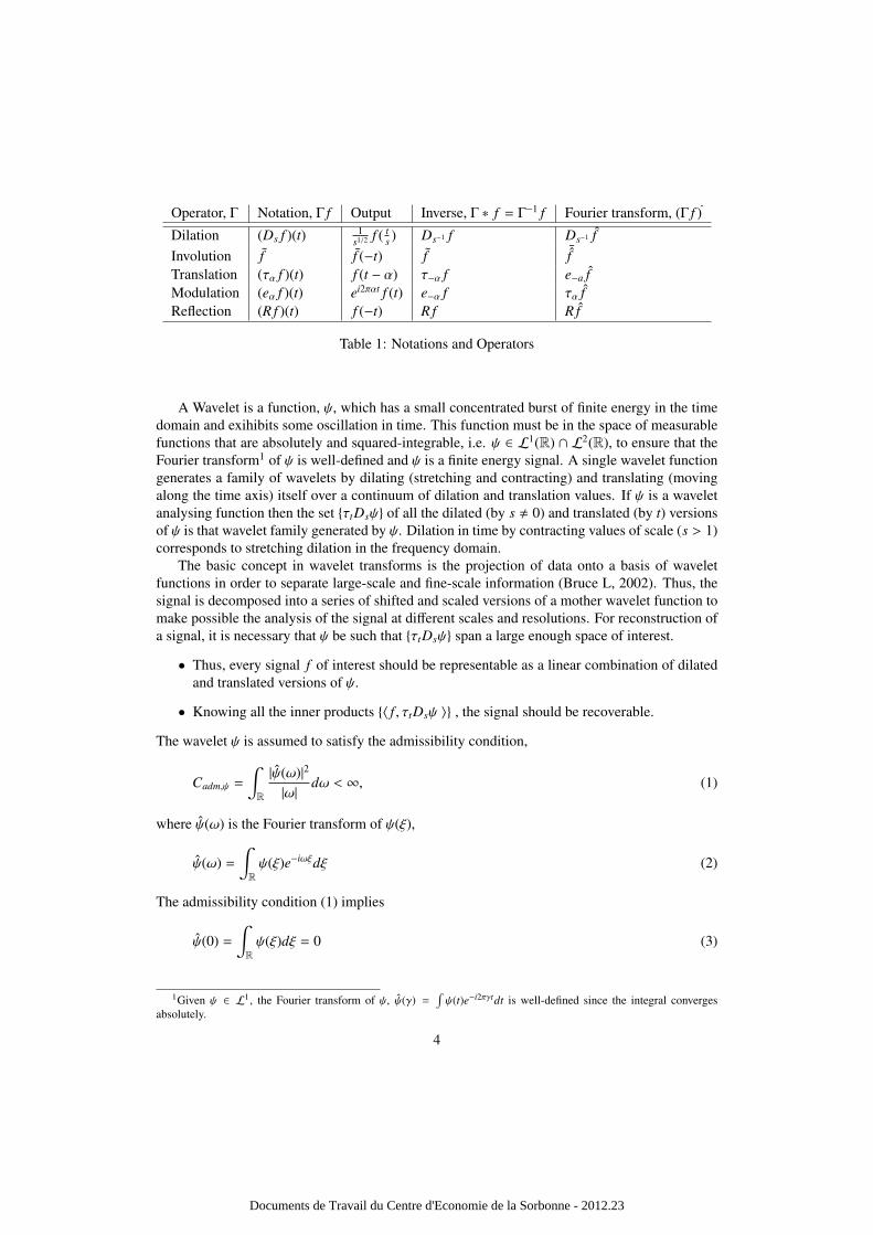
Operator, Γ Notation, Γ f Output Inverse, Γ ∗ f = Γ−1 f Fourier transform, (Γ f )

Dilation (Ds f )(t) 1s1/2 f ( t

s ) Ds−1 f Ds−1 fInvolution f f (−t) f ¯fTranslation (τα f )(t) f (t − α) τ−α f e−a fModulation (eα f )(t) ei2παt f (t) e−α f τα fReflection (R f )(t) f (−t) R f R f

Table 1: Notations and Operators

A Wavelet is a function, ψ, which has a small concentrated burst of finite energy in the timedomain and exihibits some oscillation in time. This function must be in the space of measurablefunctions that are absolutely and squared-integrable, i.e. ψ ∈ L1(R) ∩ L2(R), to ensure that theFourier transform1 of ψ is well-defined and ψ is a finite energy signal. A single wavelet functiongenerates a family of wavelets by dilating (stretching and contracting) and translating (movingalong the time axis) itself over a continuum of dilation and translation values. If ψ is a waveletanalysing function then the set τtDsψ of all the dilated (by s , 0) and translated (by t) versionsof ψ is that wavelet family generated by ψ. Dilation in time by contracting values of scale (s > 1)corresponds to stretching dilation in the frequency domain.

The basic concept in wavelet transforms is the projection of data onto a basis of waveletfunctions in order to separate large-scale and fine-scale information (Bruce L, 2002). Thus, thesignal is decomposed into a series of shifted and scaled versions of a mother wavelet function tomake possible the analysis of the signal at different scales and resolutions. For reconstruction ofa signal, it is necessary that ψ be such that τtDsψ span a large enough space of interest.

• Thus, every signal f of interest should be representable as a linear combination of dilatedand translated versions of ψ.

• Knowing all the inner products 〈 f , τtDsψ 〉 , the signal should be recoverable.

The wavelet ψ is assumed to satisfy the admissibility condition,

Cadm,ψ =

∫R

|ψ(ω)|2

|ω|dω < ∞, (1)

where ψ(ω) is the Fourier transform of ψ(ξ),

ψ(ω) =

∫Rψ(ξ)e−iωξdξ (2)

The admissibility condition (1) implies

ψ(0) =

∫Rψ(ξ)dξ = 0 (3)

1Given ψ ∈ L1, the Fourier transform of ψ, ψ(γ) =∫ψ(t)e−i2πγtdt is well-defined since the integral converges

absolutely.

4


For s restricted to R+, the condition (1) becomes

Cadm+,ψ =

∫ ∞

0

|ψ(ω)|2

ωdω < ∞. (4)

This means that the wavelet has no zero-frequency component. The value of the admissibilityconstant, Cadm,ψ or Cadm+,ψ depends on the chosen wavelet. This property allows for an effectivelocalization in both time and frequency, contrary to the Fourier transform, which decomposes thesignal in term of sines and cosines, i.e. infinite duration waves.

There are essentially two distinct classes of Wavelet transforms: the continuous wavelettransform and the discrete wavelet transform. We refer the reader to Addison, 2005; Waldenand Percival, 2000 for a review on Wavelet transforms. In this work, we mainly employ theMaximal Overlap Discrete Wavelet Transform (MODWT) and a complex continuous wavelettransform.

2.2.1. Maximal Overlap Discrete Wavelet TransformThe Maximal Overlap Discrete Wavelet Transform (MODWT), also related to notions of ’cy-

cle spinning’ and ’wavelet frames’, is with the basic idea of downsampling values removed fromdiscrete wavelet transform. The MODWT unlike the conventional discrete wavelet transform(DWT), is non-orthogonal and highly redundant, and is defined naturally for all sample sizes, N(Walden and Percival, 2000). Given an integer J such that 2J < N, where N is the number ofdata points, the original time series represented by the vector X(n), where n = 1, 2, · · · ,N, can bedecomposed on a hierarchy of time scales by details, D j(n), and a smooth part, S J(n), that shiftalong with X:

X(n) = S J(n) +

J∑j=1

D j(n) (5)

with S j(n) generated by the recursive relationship

S j−1(n) = S J(n) + DJ(n). (6)

The MODWT details D j(n) represent changes on a scale of τ = 2 j−1, while the S j(n) representsthe smooth or approximation wavelet averages on a scale of τJ = 2J−1. Gallegati and Gallegati,2007 employed this wavelet transform to investigate the issue of moderation of volatility in G-7economies and also to detect the importance of the various explanations of the moderation.

2.2.2. Continuous Wavelet Transform (CWT)The continuous wavelet transform (CWT) differs from the more traditional short time Fourier

transform (STFT) by allowing arbitrarily high localization in time of high frequency signal fea-tures. The CWT permits for the isolation of the high frequency features due to it’s variablewindow width related to the scale of observation. In particular, the CWT is not limited to usingsinusoidal analysing functions but allows for a large selection of localized waveforms that canbe employed as long as they satisfy predefined mathematical criteria (described below).

Let H be a Hilbert space, the CWT may be described as a mapping parameterized by afunction ψ

Cψ : H −→ Cψ(H). (7)5


The CWT of a one-dimensional function f ∈ L2(R) is given by

Cψ : L2(R) −→ Cψ(L2(R))f 7→ 〈 f , τtDsψ〉L2(R) (8)

where τtDsψ is a dilated (by s) and translated (by t) version of ψ given as

(τtDsψ)(ξ) =1

|s|12

ψ(ξ − t

s)

(9)

Thus, the CWT of one-dimensional signal f is a two-dimensional function of the real variablestime t, and scale s , 0. For a given ψ, the CWT may be thought of in terms of the representationof a signal with respect to the wavelet family generated by ψ, that is, all it’s translated and dilatedversions. The CWT may be written as

(Cψ f )(t, s) := 〈 f , τtDsψ〉 (10)

For each point (t, s) in the time-scale plan, the wavelet transform assigns a (complex) numericalvalue to a signal f which describes how much f like a translated by t and scaled by s version ofψ.

The CWT of a signal f is defined as

(Cψ f )(t, s) =1

|s|12

∫R

f (ξ)ψ(ξ − t

s)dξ (11)

where ψ(ξ) is the complex conjugate of the analysing wavelet function ψ(ξ). Given that ψ ischosen with enough time-frequency localization2, the CWT gives a gives a picture of the time-frequency characteristics of the function f over the whole time-scale plane R × (R\0). WhenCadm,ψ < ∞, it is possible to find the inverse continuous transformation via the relation known asCalderon’s reproducing identity3,

f (ξ) =1

Cadm,ψ

∫R2〈 f , τtDsψ〉τtDsψ(ξ)

1s2 dsdt. (12)

and if s restricted in R+, then the Calderon’s reproducing identity takes the form

f (ξ) =1

Cadm+,ψ

∫ ∞

−∞

∫ ∞

0〈 f , τtDsψ〉τtDsψ(ξ)

1s2 dsdt. (13)

Let α and β be arbitrary real numbers and f , f1, and f2 be arbitrary functions in L2(R) TheCWT, Cψ, with respect to ψ statisfies the following conditions:

1. Linearity

• (Cψ(α f1 + β f2))(t, s) = α(Cψ f1)(t, s) + β(Cψ f2)(t, s)

2The time-frequency concentrated functions, denoted T F(R), is a space of complex-valued finite energy functionsdefined on the real line that decay faster than 1

t simultaneously in the time and frequency domains. This is definedexplicitly as T F(R) := ϕ ∈ L2(R : |ϕ(t)| < η(1 + |t|)−(1+ε) and |ϕ(γ)| < η(1 + |γ|)−(1+ε) f or η < ∞, ε > 0

3This identity is also called the resolution identity.6


2. Time Invariance

• (Cψ(τβ f ))(t, s) = (Cψ f )(t − β, s)

3. Dilation

• (Cψ(Dα f ))(t, s) = (Cψ f )(αt, α−1s)

4. Negative Scales

• Cψ f (t,−s) = (CψR f )(−t, s)

The time invariance property of the CWT implies that the wavelet transform of a time-delayedversion of a signal is a time-delayed version of its wavelet transform. This serves as an importantproperty in terms of pattern recognition. This nice property is not readily obtained in the case ofDiscrete wavelet transforms (Addison, 2005; Walden and Percival, 2000).

The contribution to the signal energy at the specific scale s and location t is given by

E(t, s) = |Cψ|2 (14)

which is a two-dimensional wavelet energy density function known as the scalogram. Thewavelet transform Cψ corresponding to a complex wavelet is also complex valued. The transformcan be separated into two categories:

• Real part RCψ and Imaginary part ICψ

• Modulus (or Amplitude), |Cψ| and phase (or phase-angle), Φ(t, s),

which can be obtained using the relation :

Cψ = |Cψ|eiΦ(t,s) and Φ(t, s) = arctan(ICψ

RCψ

). (15)

In this work, we employ a complex wavelet to in order to separate the phase and amplitudeinformation. In particular, the phase information will be useful in detecting and explaining thecycles in the data.

2.2.3. Choice of WaveletThe Morlet wavelet is the most popular complex wavelet used in practice. A complex Morlet

wavelet4 (Teolis, 1998) is defined by

ψ(ξ) =1√π fb

ei2π fcξ−ξ2

fb (16)

depending on two parameters: fb and fc, which corresponds to a bandwidth parameter and awavelet center frequency respectively. The Fourier transform of ψ is

ψ(ζ) = e−π2 fb(ζ− fc)2

, (17)

4The complete Morlet wavelet can also be defined as ψ(t) = 1π1/4 (eiw0t − e−

w20

2 )e−t22 where w0 is the central frequency

of the mother wavelet. The second term in the brackets is known as the correction term, as it corrects for the non-zeromean of the complex sinusoid of the first term. In practice it becomes negligible for values of w0 > 5.

7


Figure 1: Complex Morlet wavelet with fb = 1 and fc = 0.5

which is well-defined since ψ ∈ L1(R). It can easily be shown that the Morlet wavelet (16) is amodulated gaussian function and involutive, i.e. ψ = ψ. The Fourier transform ψ has a maximumvalue of 1 which occurs at fc, since

‖ψ‖1 :=∫|ψ| = 1.

This wavelet has an optimal joint time-frequency concentration since it has an exponential decayin both time and frequency domains, meaning that it is the wavelet which provides the bestpossible compromise in these two dimensions. In addition, it is infinitely regular, complex-valued and yields an exactly reconstruction of the signal after the decomposition via CWT.

In this work, the wavelet that best detect the US business is the complex Morlet wavelet withfb = 1 and fc = 0.5. In this case, the Morlet wavelet becomes

ψ(ξ) =1√π

eiπξ−ξ2, (18)

which we will often refer to as Morlet wavelet. The nature of our choice of wavelet function andthe associated center frequency is displayed in figure 1.

2.3. Surrogate generationSurrogate time series, or ’surrogate’ for short, is non-parametric randomised linear version of

the original data which preserves the linear properties of the original data. For identification ofnonlinear/linear behavior in a given time series, the null hypothesis that the original data conformto a linear Gaussian stochastic process is formulated. An established method for generatingconstrained surrogates conforming to the properties of a linear Gaussian process is the IterativeAmplitude Adjusted Fourier Transform (iAAFT), which has become quite popular (Teolis, 1998;Schreiber and Schmitz, 1996, 2000; Kugiumtzis, 1999).

8


For |xk |, the Fourier amplitude spectrum of the original time series, X, and ck, the sortedversion of the original time series, at every iteration j, two series are generated: (i) r( j), whichhas the same signal distribution as the original and (ii) X( j), with the same amplitude spectrumas the original. Starting with r(0), a random permutation of the original time series, the iAAFTmethod is given as follows:

• compute the phase spectrum of r( j−1) → φk,

• X( j) is the inverse transform of |xk |exp(iφk), and

• r( j) is obtained by rank ordering X( j) so as to match ck.

The iteration stops when the difference between |xk | and the amplitude spectrum of r( j) stopsdecreasing. This type of surrogate time series retains the signal distribution and amplitude spec-trum of the original time series, and takes into account a possibly nonlinear and static observationfunction due to the measurement process. The method uses a fixed point iteration algorithm forachieving this, for the details of which we refer to Schreiber and Schmitz, 1996, 2000.

Wavelet-based surrogate generation is a fairly new method of constructing surrogate for hy-pothesis testing of nonlinearity which applies a wavelet decomposition of the time series. Themain difference between fourier transform and wavelet transform is that the former is only lo-calized in frequency, whereas the latter is localized both in time and frequency. The idea of awavelet representation is an orthogonal decomposition across a hierarchy of temporal and spatialscales by a set of wavelet and scaling functions.

The iAAFT-method has recently been refined using a wavelet-based approach, denoted byWiAAFT (Keylock, 2006), that provides for constrained realizations5 of surrogate data that re-sembles the original data while preserving the local mean and variance as well as the powerspectrum and distribution of the original except for randomizing the nonlinear properties of thesignal. The WiAAFT-procedure follows the iAAFT-algorithm but uses the Maximal OverlapDiscrete Wavelet Transform (MODWT) where the iAAFT-procedure is applied to each set ofwavelet detail coefficients D j(n) over the dyadic scales 2 j−1 for j = 1, · · · , J, i.e., each set ofD j(n) is considered as a time series of its own.

2.4. Optimal Embedding Parameters

In the context of signal processing, an established method for visualising an attractor of anunderlying nonlinear dynamical signal is by means of time delay embedding (Hegger R. andSchreiber, 1999). By time-delay embedding, the original time series xk is represented in theso-called ’phase space’ by a set of delay vectors6 (DVs) of a given embedding dimension, m, andtime lag, τ : x(k) = [xk−τ, · · · , xk−mτ]. Gautama T., 2003 proposed a differential entropy basedmethod for determining the optimal embedding parameters of a signal. The main advantage ofthis method is that a signal measure is simultaneously used for optimising both the embeddingdimension and time lag. We provide below an overview of the procedure:

5These are surrogate realizations that are generated from the original data to conform to certain properties of theoriginal data, e.g., their linear properties, i.e., mean, standard deviation, distribution, power spectrum and autocorrelationfunction (Schreiber and Schmitz, 1996, 2000).

6Time delay embedding is an established method for visualising an attractor of the underlying nonlinear dynamicalsignal, when processing signals with structure (Hegger R. and Schreiber, 1999).

9


The “Entropy Ratio” is defined as

Rent(m, τ) = I(m, τ) +m ln N

N, (19)

where N is the number of delay vectors, which is kept constant for all values of m and τ underconsideration,

I(m, τ) =H(x,m, τ)〈H(xs,i,m, τ)〉i

(20)

where x is the signal, xs,i i = 1, · · · ,Ts surrogates of the signal x, 〈·〉i denotes the average overi, H(x,m, τ) denotes the differential entropies estimated for time delay embedded versions of atime series, x, which an inverse measure of the structure in the phase space. Gautama T., 2003proposed to use the Kozachenko-Leonenko (K-L) estimate (Leonenko and Kozachenko, 1987)of the differential entropy given by

H(x) =

T∑j=1

ln(Tρ j) + ln 2 + CE (21)

where T is the number of samples in the data set, ρ j is the Euclidean distance of the j-th delayvector to its nearest neighbour, and CE(≈ 0.5772) is the Euler constant. This ratio criterion re-quires a time series to display a clear structure in the phase space. Thus, for time series with noclear structure, the method will not yield a clear minimum, and a different approach needs to beadopted, possibly one that does not rely on a phase space representation. When this method isapplied directly to a time series exhibiting strong serial correlations, it yields embedding param-eters which have a preference for τopt = 1. In order to ensure robustness of this method to thedimensionality and serial correlations of a time series, Gautama T., 2003 suggested to use theiAAFT method for surrogate generation since it retains within the surrogate both signal distribu-tion and approximately the autocorrelation structure of the original signal. In this Paper, we optto use wavelet-based surrogate generation method, WiAAFT by in Keylock, 2006, for reasonsalready discussed in the previous section.

2.5. ’Delay Vector Variance’ method

The Characterisation of signal nonlinearities, which emerged in physics in the mid-1990s,have been successfully applied in predicting survival in heart failure cases and also adopted inpractical engineering applications (Ho A et al., 1997; Chambers and Mandic, 2001). The ’delayvector variance’ (DVV) method (Gautama T., 2004a) is a recently proposed phase space basedmethod for signal characterisation. It is more suitable for signal processing application becauseit examines the nonlinear and deterministic signal behaviour at the same time. The algorithm issummarized below:

• For an optimal embedding dimension m and time lag τ, generate delay vector (DV): x(k) =

[xk−τ, · · · , xk−mτ] and corresponding target xk

• The mean µd and standard deviation, σd, are computed over all pairwise distances betweenDVs, ‖x(i) − x( j)‖ for i , j.

10


• The sets Ωk are generated such that Ωk = x(i)|‖x(k)− x(i)‖≤ %d, i.e., sets which consist ofall DVs that lie closer to x(k) than a certain distance %d, taken from the interval [min0, µd−

ndσd; µd +ndσd], e.g., uniformly spaced, where nd is a parameter controlling the span overwhich to perform the DVV analysis.

• For every set Ωk, the variance of the corresponding targets, σ2k , is computed. The aver-

age over all sets Ωk, normalised by the variance of the time series, σ2x, yields the target

variance, σ∗2 :

σ∗2(%d) =

1N

∑Nk=1 σ

2k(%d)

σ2x

(22)

where N denotes the total number of sets Ωk(%d)

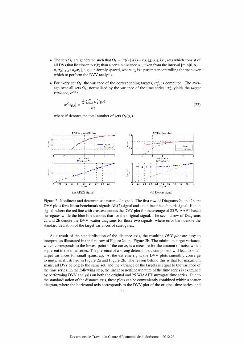
(a) AR(2) signal (b) Henon signal

Figure 2: Nonlinear and deterministic nature of signals. The first row of Diagrams 2a and 2b areDVV plots for a linear benchmark signal: AR(2) signal and a nonlinear benchmark signal: Henonsignal, where the red line with crosses denotes the DVV plot for the average of 25 WiAAFT-basedsurrogates while the blue line denotes that for the original signal. The second row of Diagrams2a and 2b denote the DVV scatter diagrams for those two signals, where error bars denote thestandard deviation of the target variances of surrogates.

As a result of the standardisation of the distance axis, the resulting DVV plot are easy tointerpret, as illustrated in the first row of Figure 2a and Figure 2b. The minimum target variance,which corresponds to the lowest point of the curve, is a measure for the amount of noise whichis present in the time series. The presence of a strong deterministic component will lead to smalltarget variances for small spans, nd. At the extreme right, the DVV plots smoothly convergeto unity, as illustrated in Figure 2a and Figure 2b. The reason behind this is that for maximumspans, all DVs belong to the same set, and the variance of the targets is equal to the variance ofthe time series. In the following step, the linear or nonlinear nature of the time series is examinedby performing DVV analysis on both the original and 25 WiAAFT surrogate time series. Due tothe standardisation of the distance axis, these plots can be conveniently combined within a scatterdiagram, where the horizontal axis corresponds to the DVV plot of the original time series, and

11


the vertical to that of the surrogate time series. If the surrogate time series yield DVV plotssimilar to that of the original time series, as illustrated by the first row of Figure 2a, the DVVscatter diagram coincides with the bisector line, and the original time series is judged to be linear,as shown in second row of Figure 2a. If not, as illustrated by first row of Figure 2b, the DVVscatter diagram will deviate from the bisector line and the original time series is judged to benonlinear, as depicted in the second row of Figure 2b.

In Figure 3 and Figure 4, we provide the structure of the DVV analysis on some simu-lated processes such as: a self-exciting threshold autoregressive process (SETAR), linear autore-gressive integrated moving average (ARIMA) signal, a Generalised autoregressive conditionalheteroskadastic process (GARCH), and a signal with a mean equation as Autoregressive (AR)process and the innovations generated from a skewed Student-t APARCH (asymmetric powerautoregressive conditional heteroskadastic) process. The interpretation of the DVV analysis isnot different from the previous illustration.

(a) DVV analysis on ARIMA(1,1,0) signal (b) DVV analysis on SETAR(2,2,2) signal

Figure 3: DVV analysis on ARIMA and SETAR signals

(a) DVV analysis on GARCH(1,1) signal (b) DVV analysis on AR(1)-t-APARCH(2,1) signal

Figure 4: DVV analysis on GARCH and AR(1)-t-APARCH(2,1) signals

12


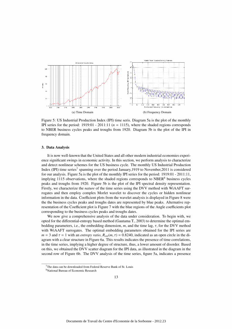
(a) Time Domain (b) Frequency Domain

Figure 5: US Industrial Production Index (IPI) time seris. Diagram 5a is the plot of the monthlyIPI series for the period: 1919:01 - 2011:11 (n = 1115), where the shaded regions correspondsto NBER business cycles peaks and troughs from 1920. Diagram 5b is the plot of the IPI infrequency domain.

3. Data Analysis

It is now well-known that the United States and all other modern industrial economies experi-ence significant swings in economic activity. In this section, we perform analysis to characterizeand detect nonlinear schemes for the US business cycle. The monthly US Industrial ProductionIndex (IPI) time series7 spanning over the period January,1919 to November,2011 is consideredfor our analysis. Figure 5a is the plot of the monthly IPI series for the period: 1919:01 - 2011:11,implying 1115 observations, where the shaded regions corresponds to NBER8 business cyclespeaks and troughs from 1920. Figure 5b is the plot of the IPI spectral density representation.Firstly, we characterize the nature of the time series using the DVV method with WiAAFT sur-rogates and then employ complex Morlet wavelet to discover the cycles or hidden nonlinearinformation in the data. Coefficient plots from the wavelet analysis is displayed in Figure 8 werethe the business cycles peaks and troughs dates are represented by blue peaks. Alternative rep-resentation of the Coefficient plot is Figure 7 with the blue regions of the Angle coefficients plotcorresponding to the business cycles peaks and troughs dates.

We now give a comprehensive analysis of the data under consideration. To begin with, weopted for the differential-entropy based method (Gautama T., 2003) to determine the optimal em-bedding parameters, i.e., the embedding dimension, m, and the time lag, τ, for the DVV methodwith WiAAFT surrogates. The optimal embedding parameters obtained for the IPI series arem = 3 and τ = 1 with an entropy ratio, Rent(m, τ) = 0.8240, indicated as an open circle in the di-agram with a clear structure in Figure 6a. This results indicates the presence of time correlations,in the time series, implying a higher degree of structure, thus, a lower amount of disorder. Basedon this, we obtained the DVV scatter diagram for the IPI data, as illustrated in the diagram in thesecond row of Figure 6b. The DVV analysis of the time series, figure 5a, indicates a presence

7The data can be downloaded from Federal Reserve Bank of St. Louis8National Bureau of Economic Research

13


http://research.stlouisfed.org/fred2/

http://www.nber.org/cycles.html

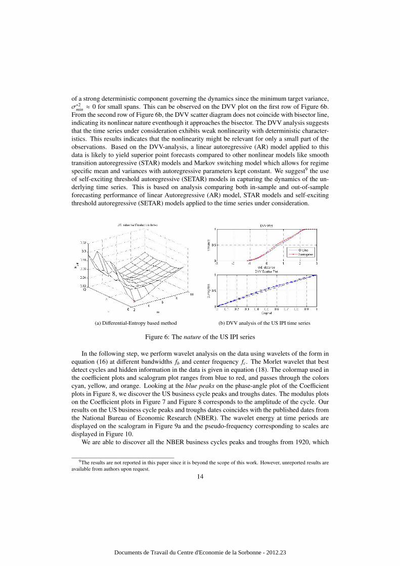
of a strong deterministic component governing the dynamics since the minimum target variance,σ∗2min ≈ 0 for small spans. This can be observed on the DVV plot on the first row of Figure 6b.From the second row of Figure 6b, the DVV scatter diagram does not coincide with bisector line,indicating its nonlinear nature eventhough it approaches the bisector. The DVV analysis suggeststhat the time series under consideration exhibits weak nonlinearity with deterministic character-istics. This results indicates that the nonlinearity might be relevant for only a small part of theobservations. Based on the DVV-analysis, a linear autoregressive (AR) model applied to thisdata is likely to yield superior point forecasts compared to other nonlinear models like smoothtransition autoregressive (STAR) models and Markov switching model which allows for regimespecific mean and variances with autoregressive parameters kept constant. We suggest9 the useof self-exciting threshold autoregressive (SETAR) models in capturing the dynamics of the un-derlying time series. This is based on analysis comparing both in-sample and out-of-sampleforecasting performance of linear Autoregressive (AR) model, STAR models and self-excitingthreshold autoregressive (SETAR) models applied to the time series under consideration.

(a) Differential-Entropy based method (b) DVV analysis of the US IPI time series

Figure 6: The nature of the US IPI series

In the following step, we perform wavelet analysis on the data using wavelets of the form inequation (16) at different bandwidths fb and center frequency fc. The Morlet wavelet that bestdetect cycles and hidden information in the data is given in equation (18). The colormap used inthe coefficient plots and scalogram plot ranges from blue to red, and passes through the colorscyan, yellow, and orange. Looking at the blue peaks on the phase-angle plot of the Coefficientplots in Figure 8, we discover the US business cycle peaks and troughs dates. The modulus plotson the Coefficient plots in Figure 7 and Figure 8 corresponds to the amplitude of the cycle. Ourresults on the US business cycle peaks and troughs dates coincides with the published dates fromthe National Bureau of Economic Research (NBER). The wavelet energy at time periods aredisplayed on the scalogram in Figure 9a and the pseudo-frequency corresponding to scales aredisplayed in Figure 10.

We are able to discover all the NBER business cycles peaks and troughs from 1920, which

9The results are not reported in this paper since it is beyond the scope of this work. However, unreported results areavailable from authors upon request.

14


Figure 7: Complex Morlet wavelet transform coefficients plots: First row is the Real and Imagi-nary parts and the second row represents Modulus and Angle coefficients. The colormap rangesfrom blue to red, and passes through the colors cyan, yellow, and orange. The blue peaks on theAngle Coefficient plot corresponds to the monthly dates for peaks and troughs of U.S. businesscycles from 1920. The corresponding amplitudes can be read from the Modulus plot.

is reported on Table 2. The Wall Street Crash of 1929, followed by the Great Depression10

of the 1930s - the largest and most important economic depression in the 20th century - arewell captured on the phase-angle coefficient plot in the figure 8 for time period (128 - 235). Thecorresponding amplitude and energy of the Great depression are represented by the cyan color onthe modulus plot in Figure 8 and the scalogram in Figure 9a respectively. The three recessionsbetween 1973 and 1982: the oil crisis - oil prices soared, causing the stock market crash areshown on the blue peaks of the phase-angle coefficient plot in the figure 8 for the time periods(659-676), (733-739), (751-767). Furthermore, the bursting of dot-com bubble - speculationsconcerning internet companies crashed is also detected for the time periods (987-995). We canobserve from Figure 9a that the scalogram reveals high energy of 0.02% at time periods (1068 -1115) corresponding to the Financial crisis of 2007-2011, followed by the late 2000s recessionand the 2010 European sovereign debt crisis. In order to compare the late-2000s financial crisiswith the Great Depression of the 1930s, we perform the wavelet analysis considering the periodof January, 1919 to December, 1939. The US business cycle peaks and troughs dates for thisperiod were clearly detected as shown on the Coefficient plots in Figure 11. Looking at Figure9b, we clearly observe high energy levels on the interval (0.02%−0.04%) for period of the GreatDepression of the 1930s. This results, as observed from the scalograms in Figure 9, providesevidence to support the claim made by many economists that the late-2000s financial crisis,also known as the Global Financial Crisis (GFC) is the worst financial crisis since the GreatDepression of the 1930s.

10The Great Depression in the United States, where, at its nadir in 1933, 25 percent of all workers and 37 percent of allnonfarm workers were completely out of work (Gene Smiley: Rethinking the Great Depression (American Ways Series)

15


Figure 8: Complex Morlet wavelet transform coefficients plots: First row is the Real and Imagi-nary parts and the second row represents Modulus and Angle coefficients. The colormap rangesfrom blue to red, and passes through the colors cyan, yellow, and orange. The blue regions on theAngle Coefficient plot corresponds to the monthly dates for peaks and troughs of U.S. businesscycles from 1920. The corresponding amplitudes can be read from the Modulus plot.

(a) Scalogram from January, 1919 to November, 2011. (b) Scalogram from January, 1919 to December, 1939.

Figure 9: The colormap of the scalograms ranges from blue to red, and passes through thecolors cyan, yellow, and orange. The bar on the left-hand side of the scalogram plot indicates thepercentage of energy for each wavelet coefficient. The scalogram in figure 9a reveals high energyof 0.02%, at time periods (1068 - 1115) corresponding to the period of late-2000s financial crisis,also known as the Global Financial Crisis. Higher energy levels on the interval (0.02%− 0.04%)can be clearly observed, in figure 9b for the Great Depression of the 1930s.

16


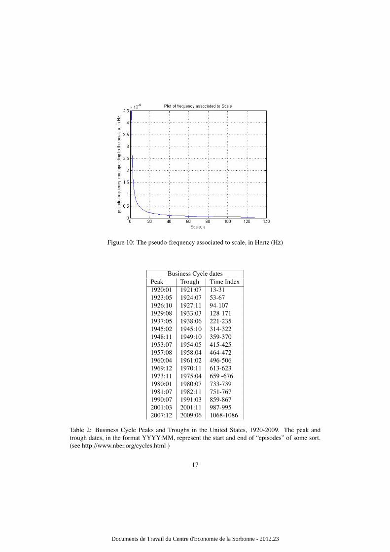
Figure 10: The pseudo-frequency associated to scale, in Hertz (Hz)

Business Cycle datesPeak Trough Time Index1920:01 1921:07 13-311923:05 1924:07 53-671926:10 1927:11 94-1071929:08 1933:03 128-1711937:05 1938:06 221-2351945:02 1945:10 314-3221948:11 1949:10 359-3701953:07 1954:05 415-4251957:08 1958:04 464-4721960:04 1961:02 496-5061969:12 1970:11 613-6231973:11 1975:04 659 -6761980:01 1980:07 733-7391981:07 1982:11 751-7671990:07 1991:03 859-8672001:03 2001:11 987-9952007:12 2009:06 1068-1086

Table 2: Business Cycle Peaks and Troughs in the United States, 1920-2009. The peak andtrough dates, in the format YYYY:MM, represent the start and end of “episodes” of some sort.(see http://www.nber.org/cycles.html )

17


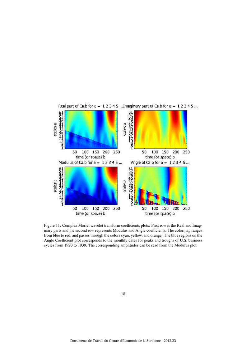
Figure 11: Complex Morlet wavelet transform coefficients plots: First row is the Real and Imag-inary parts and the second row represents Modulus and Angle coefficients. The colormap rangesfrom blue to red, and passes through the colors cyan, yellow, and orange. The blue regions on theAngle Coefficient plot corresponds to the monthly dates for peaks and troughs of U.S. businesscycles from 1920 to 1939. The corresponding amplitudes can be read from the Modulus plot.

18


4. Conclusion

We have utilised the Delay Vector Variance(DVV) method and Wavelet analysis to charac-terize the nature of the US Industrial Production Index data. It has been shown that the DVVmethod and the Complex Morlet Wavelet can serve as an alternative way to detect and char-acterize nonlinearity schemes in the US business cycle. In particular, we have shown that thewavelet approach serves as an alternative methodology for turning-point detection in businesscycle analysis.

References

Addison, P. S., 2005. Wavelet transforms and ecg: a review. Physiological Measurement 26, 155–199.Aguiar-Conraria, Soares, 2011. The continuous wavelet transform: A primer, nIPE – WP 16.Bruce L, Koger C, J. L., 2002. Dimentionality reduction of hyperspectral data using discrete wavelet transform feature

extraction. IEEE Transactions on Geoscience and Remote Sensing 40, 2331–2338.Casdagli, M. C. . W. A. S., 1994. Exploring the continuum between deterministic and stochastic modelling, in time series

prediction: Forecasting the future and understanding the past. Reading, MA: Addison-Wesley, 347–367.Chambers, D., Mandic, J., 2001. Recurrent neural networks for prediction: learning algorithms architecture and stability.

Chichester, UK: Wiley.Gallegati, M., 2008. Wavelet analysis of stock returns and aggregate economic activity. Computational Statistics and

Data Analysis 52, 3061–3074.Gallegati, M., Gallegati, M., 2007. Wavelet variance analysis of output in g-7 countries. Studies in Nonlinear Dynamics

and Econometrics 11 (3), 6.Gautama T., Mandic D.P., V. H. M., 2003. A differential entropy based method for determining the optimal embedding

parameters of a signal. In Proceedings of ICASSP 2003, Hong Kong IV, 29–32.Gautama T., Mandic D.P., V. H. M., 2004a. The delay vector variance method for detecting determinism and nonlinearity

in time series. Physica D 190 (3–4), 167–176.Gautama T., Mandic D.P., V. H. M., 2004b. A novel method for determining the nature of time series. IEEE Transactions

on Biomedical Engineering 51, 728–736.Hegger R., H. K., Schreiber, T., 1999. Practical implementation of nonlinear time series methods: The tisean package.

Chaos 9, 413–435.Ho A, K. Moody, G. P., C. Mietus, J. Larson, M. L., Goldberger, D., 1997. Predicting survival in heart failure case

and control subjects by use of fully automated methods for deriving nonlinear and conventional indices of heart ratedynamics. Circulation 96, 842–848.

Kaplan, D., 1994. Exceptional events as evidence for determinism. Physica D 73 (1), 38–48.Keylock, C., 2006. Constrained surrogate time series with preservation of the mean and variance structure. Physical

Review E 73, 036707.Kugiumtzis, D., 1999. Test your surrogate data before you test for nonlinearity. Physics Review E 60, 2808–2816.Leonenko, N., Kozachenko, L., 1987. Sample estimate of the entropy of a random vector. Problems of Information

Transmission 23, 95–101.Schreiber, T., Schmitz, A., 1996. Improved surrogate data for nonlinearity tests. Physics Review Lett. 77, 635–638.Schreiber, T., Schmitz, A., 2000. Surrogate time series. Physica D 142, 346–382.Stock, M. W., Watson, J. H., 1999. Forecasting inflation. Journal of Monetary Economics 44 (2), 293–335.Teolis, A., 1998. Computational signal processing with wavelets. Birkhauser.Terasvirta, T., September 2011. Modelling and forecasting nonlinear economic time series, wGEM workshop, European

Central Bank.Walden, D., Percival, A., 2000. Wavelet Methods for Time Series Analysis. Cambridge: Cambridge University Press.Whitcher, B. G. P., Percival, D., 2000. Wavelet analysis of covariance with application to atmospheric time series. Journal

of Geophysical Research 105, 14941–14962.

19
