L/

jLT-CHNICA[ REPORT SL-90-1

EVALUATION OF NONLINEAR CONSTITUTIVE-- PROPERIEIS OF CONCRETE

Crles Dean Norman

0 StwLctu!res Laboratory

DE!-ARTMENT OF THE ARMY0< ,, EEr.'-irment Station, Corps of Engineers

Road, Vicksbura. Mississippi 39180-6199

DTICELECTE

MARO 1 99 U

February 1990

c r) ReportF i-a . ...S'r~jvf JrI't*

Ballistic Missile OfficeNorton Air Force Base, California 92409-6468

and

Defense Nuclear AgencyWashington, DC 20305-1000

LABC. - i,

190 02 "S.. 7

When this report is no longer needed return it tothe originator.

The findings in this report are not to be construed as anofficial Department of the Army position unless so

designated by other authorized documents.

The contents of this report are not t. .)e used foradvertising, publication, or promotional purposes.Citation of trade names does not constitute anofficial endorsement or approval of the use of such

commercial products.

cassI fiedSECURITY CLASS41'CAT ON COp -_ S A E

Form ApproveoREPORT DOCUMENTATION PAGE ORBNo 0704 "'88

!a REPORT 5EC RiTy C-ASS :CA '

10 RESTRIC':vE MARKNGS

Unclassified2a SECURITY CLASS.FCA- 0% . _ -,ORT,T 3 DISTRIBor;ON, AVALAB;UTY OF - "ORT

20 DECLASSNFCATONDOcPNG ScEouE pproved for public release; disc:ribution.

inlimited.4 PERFORMING ORGAN ZA- ON 'REPORT %NMeER(S) 5 MONITORING ORGANIZATON REPORT NUMBER(S)

Technical Report SL-JO-1

(CTIAC Report No. )

6a NAME OF PERFORMING ORGANiZATON 6b OFF-CE SYMBOL 7a NAME OF MONITORING ORGAN ZATION

USAEWSES (If applicable)

Structures Laboratory CEWES-SC-R

6c_ ADDRESS IC,ty, State, and ZIPCode) 7b ADDRESS (City, State, and ZIP Coae)

3909 Halls Ferry RoadVicksburg, MS 39180-6199

8a NAME OF PUNDING SPONSOR'NG Bb OFFICE SYMBOL 9 PROCUREMFNT INSTRUMENT

IDENTFICATiON NUMBERORGANIZATION (If applicable)

8c_ ADDRESS (City, State, and ZIP Ccife) 10 SOURCE OF FUNDING NUMBERS

Norton Air Force Base PROGRAM PROjECT TASK WORK

CA 92409-6468 ELEMENT NO NO NO ACCFSS G. NO

11 TITLE (Include Security Clasp.fication)

Evaluation of Nonlinear Constitutive Properties of Concrete12 PERSONAL AUTHOR(S)

Norman, C. Dean1 3a TYPE OF REPORT 1 3b TIME COVERED 14 DATE OF REPORT (Year, Month, Day) 15 PAGE COUN4T

Final Report FROM JCt 193/TOM-. 198 February 1990 216

16. SUPPLEMENT ARY NOtATION

Available from National Technical Information Service, 5285 Port Royal Road-.Springfield,

VA 22161.17 COSATI CODES SUBJECT TERMS (Continue on reverse if necessary and rdentf' .' block nu?' r

FIELD GROUP SUB-GROUP Ctomputer models, Material propertle\

IConcrete, Plasticity sr-r.

IConstitutive models , " " \19:#BSTRACT (Continue on reverse if necesuar 4nd identify by block number)

3his report describes the development of a methodology that allows for th ectiv.

evaluation o(f__the predictive capabilities of concrete constitutive models

'The structural analysis and design of concrete structures is o ten based on large-scale

finite element computations. A key component of the finite element method is the constitu-

tive model that is usually selected and calibrated based on a few simple tests. The primary

reason for this is the lack of understanding of the complex response features of concreteand numerical difficulties eucuuntered when attempting to model these ttatures. Also, the

error in response predictions due to an inappropriate constitutive model is difficult to

define i. a complex large-scale structural analysis problem.

(Continued)

20 , j'=:BUTION/AVAILABILiTY OF ABSTRA- 21 ABSTRACT SECURiTY C_.ASSiFCATION

[] UNCLASSIFIE>IUNLMITED M SAME T [: OTIC USERS Unclassified

22a "4AME OF RESPONSIBLE 'NDIViDUAL 22b TELEPHONE(inclule AreaCode) 22c OFFICE SYMBOL

D Form 1473, JUN 86 Previous editions ,# obsolete SECURITY CLASSIFICATION OF THIS PAGE

Unclassified

.nclassifited

19. ABSTRACT (Continued).

The method of evaluation, as developed herein, consists of the following steps:

1. The design and execution of a series of material properties tests which providedata sulficient for the calibration of the constitutive model under consideration.

2. Calibration of the model using the data developed in Step L.

3. Design and execution of the series of verification tests which provide data suffi-cient for defining key complex material response features that are to be modeled.

4. Direct comparison of model predicted response with experimental measurementsthrough the use of a constitutive driver.

The constitutive models were evaluated, the Fracture Energy Based Model (FEBM) and the Endo-chronic Concrete Plasticity Model (ECPM).

While there are very many constitutive models for concrete currently available i: theliterature, it was not possible within the sc'p of this research project to evaluate all ofthem, although the methodology presented should be equally applicable to all. The selectionof the FEBM and the ECPM is not intended to endorse these models as the better ones. Theresults show that, although they are able to predict qualitatively some key response fea-tures observed in the verification tests, they fail to predict accurately other responsefeatures. These models were selected because they are two of the more recent and comprehen-

sive ones and also the theoretical development of the two is significantly different.

Unclassified

SECUAITY CLAISIPICATIOM OP T'12 PAGE

PREFACE

The research reported herein was conducted at the US Army Engineer

Waterways Experiment Station (USAEWES), Structures Laboratory (SL), under the

sponsorship of the Ballistic Missile Office (BMO) of the US Air Force, Norton

Air Force, Base, CA. The general concept and financial support for this study

were further promoted by the Defense Nuclear Agency (DNA). Funds for the pub-

lication of the report were provided from those made available for operation

of the Concrete Technology Information Analysis Center (CTIAC) at WES, SL.

This is CTIAC Report No. 86.

The BMO project officer was LT Rob Michael and the technical director

was Dr. Mike Katona, TRW Systems, Norton Air Force Base. LTC Don Gage and

CPT John Higgins, US Air Force, and Dr. Kent Goering, DNA, were involved in

this project through their agencies.

Dr. C. Dean Norman, Concrete Technology Division (CTD), SL, WES, pre-

pared this report in partial fulfillment of the Ph.D. requirements from the

University of Texas at Austin. The University's supervisory committee

included Drs. Jose Roesset, Eric Becker, John Tassoulas, Phillip Johnson, and

James Jirsa. The late Dr. Nathan M. Newmark accepted membership on the com-

mittee but was unable to serve.

The work was accomplished during the period October 1987 through May

1989 at WF under the general supervision of Mr. Bryant Mather, Chief, SL, and

Mr. Ken Saucier. Chief, CTD. Messrs. Michael I. 1Hammons and Donald M. Smith,

CTD, conducted tests, daca reduction, general review, and discussions of test

results. Ms. Sharon Garner, CTD, was directly responsible for modifying and

developing effective software in the WES Constitutive Driver used in the eval-

uation of constitutive models for this study. Dr. John Peters, Geotechnical

Laboratory, provided many helpful discussions, and Messrs. Dan Wilson and

James Shirley, CTD, SL, performed outstanding work through the test program

designed and directed by Dr. Norman. The technical report was published by

the Information Technology Laboratory, WES.

COL Larry B. Fulton, EN, is the Commander and Director of WES.

Dr. Robert W. Whalin is the WES Technical Director.

i

Table of Contents

Page

Preface ............................................................... i

Conversion Factors, Non-SI to SI (Metric) Units of Measurement ..... iii

1. Introduction ........................................................

1.1 Background .................................................. 1... ..1.2 Objectives....................................................... 51.3 Scope ........................................................... 61.4 Cutline .......................................................... 6

2- Stress Strain Response of Concrete ............................... 11

2.1 General ........................................................ 112.2 Loaders, Test Devices, nnd Instrumentation ................... 152.3 Unconfined Compression Tests ................................... 21

2.4 Hydrostatic Compression Test ................................... 262.5 Uniaxial Strain Test ....... .................................. 27

2.6 Triaxial Compression Test.. ................................... 302.7 Verification Tests ............................................. 38

3. Constitutive Equations ............................................ 56

3.1 General ........................................................ 56

3.2 Linear Elasticity .............................................. 573.3 Conventional Plasticity ........................................ 64

3.4 Material Stability Postulates, Uniqueness ................... 763.5 Examples of Hardening and Softening Formulations ............ 81

3.6 Fracture Energy Based Model .................................... 89

3.7 Endochronic Plasticity Mode] ................................. 104

4. Comparison of Model Predictions Versus Test Results ............ 128

4.1 General ....................................................... 1284.2 WES-Constttutive Driver ........................................ 1284.3 Comparison of Model Predictions with WES Tests .............. 133

4.4 FEBM and ECPM - VT4-1, VT4-2, VT4-3 ........................... 190

4.5 FEBM and ECPM - VT5-1, VT5-2, VT5--3............................ 196

5. Conclusions/Recommendations ....................................... 200

5.1 Summary ........................................................ 2005.2 Conclusions ................................................... 201

5.3 Recommendations..... ......................................... 205

6. Bibliography ...................................................... 208

ii

CONVERSION FACTORS, NON-SI TO SI (METRIC)

UNITS OF MEASUREMENT

Non-Si units of measurement can be converted to ST (metric) -unis as follows:

Multiply By To Obtain

inches 25.4 millimetres

feet per second 0.3048 metres per second

kips (1,000-lb mass) 453.59237 kilograms

kips (force) per square inch 6.894757 megapascals

pounds (force) 4.448222 newtons

pounds (force) per square inch 0.006894757 megapascals

Aooesion For

NTIS GRA&I

DTIC TAR 0UnannuncedJustlfloatia_

Dist

Evaluation of Non-linear Constitutive

Properties of Concrete

Chapter 1: Introduction

1.1 Background.

The complex stress-strain response features of concrete have

been studied and discussed considerably in the technical literature

with summaries of these results presented in many textbooks (e.g.,

Neville ( 1 , Chen 2 ) , etc.). Some of the key response features which

can have a significant impact on the development of constitutive mod-

els include:

a. The dependence of yield or maximum strength surfaces on con-

fining stress.

b. The occurrence of plastic volume change and in particularplastic volume change due to pure shear loading.

c. Strain softening under displacement controlled loadingconditions.

The general effects of these features on stress strain response are

presented in Figures 1.1 through 1.3. Figure 1.1 shows the effects

of increasiag confining stress on the stiffness and strength of a

concrete specimen under increasing axial stress. Figure 1.2 shows

the increase in plastic volume change (compaction) due to pure sheer

loading, while Figure 1.3 presents test results indicating strain

softening at low confining stress levels. From a qualitative stand-

point, these response features can be partially explained by consid-

ering the internal structure of concrete at the three-phase level

(aggregate, cement matrix, air voids). Such a description is pre-

sented graphically in Figure 1.4a, which represents a specimen from a

well proportioned concrete mixture which has been properly consoli-

dated and cured. Furthermore, it is assumed that the nominal maximum

size of the aggregate is small compared to the minimum dimension of

*Numbers in parenthesis indicate references presented at the end of

the dissertation.

the specimen so that on any plane cut through the specimen, the nor-

mal and shear stress distributions can be effectively represented as

a constant average value (made up of the contributions from the

aggregates, cement paste, and voids). In this -nloaded specimen,

some cracks will be observed, primarily at the aggregate-cement

matrix interface. These cracks develop during the curing process and

are primarily due to differences in aggregate and cement paste stiff-

nesses, shrinkage, and thermal properties. When compressive axial

stresses alone are applied in the vertical direction (Figure 1.4b)

and monotonically increased, microcracks will begin to propagate

through the cement matrix which results in a net decrease in the

stiffness of the specimen. These cracks will be oriented primarily

vertically on the exposed outer surface due to the tensile strains

developed in the circumferential direction. Cracks will coalesce

into longer vertical cracks as the stress is increased up to some

maximum value where failure will occur. Actually, if the load is

applied in displp-ement control, the load will, from this maximum

value, decrease as the axial strain continues to increase, however,

significant specimen cracking and damage, will be very apparent). On

the other hand, if hydrostatic stresses are applied to the test spec-

imen (Figure 1.4r), the initial cracks (Figure 1.4a) will begin to

close so that shear stresses can be transferred more effectively

across the aggregate-cement paste interfaces. As the hydrostatic

stress increases, the normal component of stress on a typical aggre-

gate surface element will increase, and therefore the frictional

shear strength at this point will increase. In general, this confin-

ing stress effect is to increase the effective moduli of the specimen

as well as the maximum strength and yield surfaces.

As the hydrostatic stresses increase, the volume decreases (com-

paction), and part of this volume change is irrecoverable (plastic)

as shown in Figure 1.2. This, of course, is unlike the response of

most metals where essentially no plastic volume change occurs as all

plastic strains are associated with shear due to slip between grain

3

boundaries. This difference in response between polycrystalline

metals aui concrete is primarily due to the more heterogeneous

internal structure of concrete. As voids and microcracks close under

increasing hydrostatic stress, the volume decreases. However, the

volume at a particular level of hydrostatic stress is not necessarily

a minimum for that level of stress due to the fact that microcracks

and voids can still exist due to the complicated microstress distri-

bution in the specimen which can cause bridging around local discon-

tinuities. As a pure shear stress is applied (at constant

hydrostatic stress), a further decrease in volume occurs (Fig-

ure 1.2). This feature can be explained by approximating concrete,

at a particular level of hydrostatic stress, as a loosely packed sys-

tem of incompressible spheres. If any pure shear distortion is

applied to the system, the volume must decrease. Also, one should

consider the shearing effect of concrete along a rough crack where

each application of shear tends to smooth the crack and therefore

decrease the volume of the specimen containing the crack.

The third response feature listed above (strain softening) has

received considerable discussion in the past and continues to be vig-

orously debated. The main issue is: "Should strain softening be

considered a property of the material or a result of the structural

geometry and loading conditions or, the test specimen?" The later

argument is generally based on: (a) the frequent observation of bar-

reling of test specimens which indicates that unwanted shear stresses

are being applied at the specimen boundaries and that the stress and

strain state in the specimen are not homogeneous; (b) significant

cracking of the test specimen, which again implies an inhomogeneous

stress state in the material; (c) local inhomogeneities are observed

within the test specimen and are usually associated with shear band-

ing, etc. The central question concerning softening is localization,

which implies that the assumption of a homogeneous continuum is not

valid. If, on the other hand, test results are interpreted so that

strain softening is to be considered a material property: (d) the

4

applied stresses at the specimen boundaries should be uniform, and

the current specimen geometry must be given as a constant times the

initial geometry; (e) the internal damage or response inechanisms

(i.e., fracture, void closure, etc.) should be uniformly distributed

over the specimen volume and not localized in bands of specific

regions. Figure 1.4d presents conceptually what might occur in a

test specimen during a softening test. The main point here is that

fractures in aggregates, void closures etc. are uniformly distributed

throughout the specimen volume.

The complex response features discussed here present special

problems for constitutive models. The pressure sensitivity of the

yield surface simply means t!lat yield and maximum strength surfaces

must be defined in terms of the confining stress level. The plastic

volume change problem is Lsually addressed, with varying degrees of

success, by defining yield surfaces which close on the hydrostatic

axis or by the use of cap models. When the formei method, to account

for volume change, is used, constitutive models tend to overpredict

lateral strains on many stress paths. To correct this problem, a

nonassociated flow rule can be Lsed which in effect changes the

direction of the plastic strain vector and can therefore reduce the

lateral strain component.

When strain softening is modeied as a material property, the

approach used generally is to degrade or damage the maximum strength

surface according to some rule which relates decrease in strength

(or, say, cohesion) to a softening parameter (e.g. plastic strains)

as total strains continue to increase under decreasing load.

Once constitutive models are developed which reasonably predict

these complex response features, other problems are encountered when

these models are implemented and used in dynamic finite-element

codes. The nonassociated flow rule results in a nonsymmetric mate-

rial stiffness matrix which can cause a significant Increase in com-

putational time. Also, realistic load paths can be defined along

which the nonassociated model will become unstable according to

5

certain material stability postulates. Strain softening models also

violate material stability postulates which can result in problems 3f

numerical instability and nonunique solutions. Generally, softening

and non-associated flow models tend to be !tndesirably sensitive to

small variations in prescribed initial conditions for dynamics

problems.

If a particular response feature is to be effectively modeled,

then the basis for the development of the model should be sound

repeatable material properties test data completely def .ing that

response feature. On the other hand, material stability postulates

should be considered when appropriate but Fhould not be the driving

force in the development of the model. More specifically, the com-

plex material response features of concrete to be vsed in a particu-

lar structure should be evaluated through a carefully planned

laboratory material properties test program, designed to subject the

material to stress and strain histories similar to those whi1i will

occur at critical regions in the structure under the design loads.

Furthermore, generic tests (e.g., uniaxial strain, unconfined com-

pression, etc.) should be conducted to determine basic material

response characteristics, validity of homogeneity and isotropy

assumptions, and values for parameters used to calibrate constitutive

models of interest. Finally, the concrete material should be sub-

jected to complex load path tests, which can be used to evaluate the

consistency and predictive capability of potential concrete constitu-

tive models.

1.2 Objectives

The objectives of this rebearch are:

a. The development of a methodology for evaluating constitutivemodels for plain concrete.

b. The application of this methodology in the evaluation of twoadvanced -onstitutive models.

6

1.3 Scope

The method of evaluation, as developed herein, consists of the

following steps:

1. The design and execution of a series of material propertiestests which provide data sufficient for the calibration ofthe constitutive model under consideration.

2. Calibration of the model using the data developed in step 1.

3. Design and execution of a series of verification tests whichprovide data sufficient for defining key complex materialresponse features that are to be modeled.

4. Direct comparison of model predicted response with experi-

mental measurements through the use of a constitutive

driver.

The two constitutive models to be evaluated are the Fracture Energy

Based Model (FEBM)(3) and the Endochronic Concrete Plasticity Model

(ECPM)(4).

While there are very many constitutive models for concrete, cur-

rently available in the literature, it was not possible within the

scope of this research project to evaluate all of them, although the

methodology presented should be equally applicable to all. The

selection of the FEBM and the ECPM is not intended to endorse these

models as the better ones. The results show that although they are

able to predict qualitatively some key response features observed in

the verification tests they fail to predict accurately other response

features. These models were selected because they are two of the

more recent and comprehensive ones and also the theoretical develop-

ment of the two is significantly different.

1.4 Outline

In Chapter 2, general stress-strain response features of con-

crete will be discussed along with some of the implications of strain

softening. Loaders and test devices that were used in generating

test results for this research project along with instrumentation

used are then discussed. Finally calibration and verification test

results are presented and discussed. Basic concepts of elasticity

7

and plasticity are presented in Chapter 3 with emphasis on generaliz-

ing the results observed in simple material-properties tests. Also,

in Chapter 3, a detailed derivation of the equations for the FEBM and

the ECPM are presented and the calibration of model parameters is

discussed. In Chapter 4, the two models are calibrated, exercised

against the verification tests results, and comparisons of tests

results versus model predictions are made. Conclusions and recom-

mendations for future research are presented in Chapter 5.

Maximum strengthi

X Icesing

confining stress

< i Stiffness

Axial strain

Figurel.1.Effects of confining stress on maximum strength

and stiffness.

'H3

Cd

141Lr C

-4 W -4E a.-C

0 0 u

"-4 Q00 =2

Ctc $-4 0En 0 -0 C

cz m > 41

AJ wOct

00

Aj to

co Uo

0

ssails 01. lelsolPAH

Airvoid

0 _ _ V _-Initial

crack

12 Cementmatrix

Aggregate

00

Q

(a) Unloaded test specimen.

04

(b)Cracks observed in unconfinedcompression test.

Figure 1.4.Internal characteristics of concrete(sheet 1 of 2).

10

66N

4D)

0I

og. 430°

(c)Crack and void closure dueto nydrostatic stresses.

~e 0

(d)Aggregate fracture,softeningconcept.

Figure 1.4.Internal characteristics of concrete(sheet 2 of 2).

11

Chapter 2

Stress Strain Response of Concrete

2.1 General

In Chapter 1, a general discussion was presented concerning prob-

lems encountered in large scale structural analysis of critical struc-

tures and questions many researchers have regarding various stress

strain response phenomena of concrete. Considerable experimental

data exist for concrete subjected to one dimensional and axisymmetric

load. Also several studies have been directed at strain softening,

biaxial stress loading and fully three dimensional stress loading.

Results from many of these test programs axe summarized and discussed

by Hegemier, et al. (5). Green and Swanson (6) conducted an

extensive study of the general constitutive properties of concrete at

intermediate pressure levels (i.e. 10 - 12 ksi) while Van Mier (7)

addressed strain softening under multiaxial loading conditions.

Gerstle et al. (8) through a cooperative research effort showed the

sensitivity of tests results to test devices (boundary conditions)

and test procedures. The vast majority of the existing test data is

based on simple or proportional load paths (i.e. the ratio of the

applied stresses remains constant). In this Chapter, specific

stress-strain response characteristics of concrete for simple and

complex load paths will be discussed. Furthermore, an attempt is

made to show that high quality, repeatable, and consistent test data

can be obtained for well prepared concrete specimen and furthermore

these data can and should be used in calibrating constitutive models.

Nominal unconfined compressive strengths for concretes tested in this

study range from f' = 2 ksi to f' = 7 ksi. It is not intended toc c

present herein a broad discussion of the many different complex

response characteristics of concrete, but rather to discuss those

features which are of primary importance in constitutive modeling in

general and specifically for the fracture energy based model and the

endochronic model. Essentially two types of tests will be discussed,

12

calibration tests and verification tests. Calibration tests are

conducted to determine values for parameters or coefficients used in

the mathematical formulation of a particular model. Verification

tests are designed to evaluate specific predictive capabilities of a

constitutive model. Obviously a calibration test for one model might

serve as a verification test for another model.

Before discussing test results it is important to keep in mind

that in a test we are measuring quantities such as force, (F), pres-

sure (P), and displacement (U), then dividing these (i.e. force and

displacement) by initial areas A and lengths L to obtain stress and0 0

strain. The equations we use are of course

STRESS = F / A (1)

STRESS = U / L0

The validity of using these equations to interpret or infer material

constitutive properties should be determined based on the following

conditions (Pariseau (9)):

1. Test specimen must be homogeneous

2. A homogeneous state of stress must exist in the specimen atall times.

3. No significant changes in specimen geometry can occur duringa test.

When these conditions are met one can reasonably assume constitutive

properties derived from equation (1) are real material properties.

Furthermore, if an appropriate number of tests are conducted along

load paths which capture the key response features of the material

one can construct rational constitutive models which effectively

represent the material response under a wide range of load histories.

If in the other hand these conditions are not met, one must be care-

ful in inferring material properties from equation (1) and in using

constitutive models constructed from such tests. The degree to which

the above conditions are met has special significance in interpreting

13

strain softening as a material response phenomenon or a structural

response feature. When concrete is modeled as a homogeneous, isotro-

pic material the assumption is made that the aggregates and pores are

randomly distributed throughout the cement paste matrix and that the

microcrack surface and width is relatively small when considering a

representative volume of the material. This representative volume in

general must be large enough so that the effects of stress concen-

trations, and any other discontinuities in the material can be

smeared over the volume so that an equivalent homogeneous stress and

strain state can be determined which effectively characterizes all

the important features of material response. The reason for con-

ducting material properties tests is precisely to measure these

stress and strain states along load paths which are critical consid-

ering the application. At high stresses and especially in the soft-

ening region the validity of assumptions of homogeneity become more

and more questionable. Many researchers have pointed out that at

ultimate strength and in the softening region there are localizations

of damage (eg. shear banding) and that test specimens exhibiting

these effects must be considered structural elements and not as mate-

rials subjected to states of homogeneous stress and strain.

Bazant (10) found that strain softening can be observed only when

local inhomogeneities exist in a material. The question i6, how

significant are the inhomogeneities in terms of the effects they have

on stress-strain response features of interest. Once this question

is answered one can determine what conditions (e.g. inhomogeneities)

must be considered in constructing a rational constitutive model for

a particular problem. Local inhomogeneities lead to strain softening

which can be identified as a material instability according to

Drucker's postulates (see Chapter 3). Drucker (17) points out

"Philosophically, perhaps, all macroscopic syptems are stable in the

sense that if all conditions are or could be taken into account the

complete behavior of the system could be followed in detail...

Instability as normally understood may arise when some but not all of

14

the attributes of a system are considered." For strain softening in

concrete the instability is due to the assumptions that the stress

strain response is rate independent and homogeneous.

In this chapter, loaders, test devices, and instrumentation com-

monly used in conducting material property tests will be discussed

(Section 2.2). The location of the loaders and test devices and the

laboratories where different tests were conducted is identified in

section titles (i.e. Waterways Experiment Station (WES); the Univer-

sity of Eindhoven, Netherlands (UEN); and the University of Colorado,

Boulder (UCB)). Calibration tests are discussed in Sections 2.3

through 2.6 and verification tests are discussed in 2.7.

15

2.2 Loaders, Test Devices, and Instrumentation

2.2.1 100-kip Servo-Controlled Hydraulic Loader (WES)

The 100-kip servo-hydraulic loader is capable of applying ten-

sile or compressive loads up to a maximum level of 100,000 lb. The

loader can be manually or computer controlled to produce a desired

load or displacement rate. The input to the servo-control unit is

produced by an arbitrary digital function generator which can be pro-

grammed to produce an infinite number of load or displacement his-

tories. The applied force is measured by a load cell while the

displacement of the loader head is measured by an internal linear

variable displacement transducer (LVDT). Strains are usually mea-

sured by epoxy-backed constantan resistance strain gages bonded to

the specimen with high-strength strain-gage adhesive. Unconfined

compression tests, tension tests, and some low confinement triaxial

tests can be conducted in this loader.

2.2.2 440-kip Universal Testing Machine (WES)

The 440-kip loader can apply tensile or compressive loads up to

a maximum of 440,000 lb. The machine is displacement controlled by

manually adjusting hydraulic valves to achieve the desired displace-

ment rate. The axial load is measured by an internal load cell while

displacements are measured by an external LVDT across the loading

heads. Strains are usually measured by strain gages bonded to the

specimen. This machine is used to conduct unconfined compression

tests and cylindrical triaxial compression tests.

2.2.3 2400-kip Loader (WES)

The 2400-kip servo-hydra,,lic loader can apply tensile or com-

pressive loads up to a maximum of 2,400,000 lb. The load or dis-

placement rate are controlled by an analog function generator capable

of ramp, sine, or triangular functions. The load is measured by an

internal load cell while the displacements are measured by an

16

external LVDT. This device is used to conduct unconfined compression

tests, cylindrical triaxial tests, and multiaxial compression tests.

2.2.4 40-ksi Cylindrical Triaxial Chamber (WES)

The 40-ksi cylindrical triaxial test device is capable of con-

ducting multiaxial tests on nominal 2.125-inch diameter by 3.5-inch

long cylindrical specimens at confining stresses up to 40,000 psi and

axial stresses up to 125,000 psi. Figure 2.1(a) shows a cross-

section of the device. The confining pressure is developed by a

manually controlled, air-driven hydraulic pump rated at 75,000 psi.

The fluid used in the device is a low-viscosity white mineral oil.

Eight 7/8-inch diameter bolts clamp the upper and lower platens

together and carry the loads produced by the fluid pressure against

the upper and lower cell caps. The device has the capability to exit

up to four channels of instrumentation through Fusite-type fittings

in the base.

In preparing for a test, hardened steel end caps were placed on

each end of a specimen. The specimen was subsequently encased in an

impermeable 60 durometer neoprene membrane. Hose clamps were used to

secure the membrane at each end of the specimen. The jacketed speci-

men was placed in the device, and the device was completely assem-

bled. This assembly was then moved as a unit and placed in the

440-kip universal testing machine. A swivel was placed on the top of

the ram to compensate for any eccentricities in the device or the

testing machine.

2.2.5 30-ksi Multiaxial Test Device (WES)

The 30-ksi multiaxial test device is used in conjunction with

the 2400-kip universal testing machine to test 6-inch by 6-inch by

36-inch rectangular prismatic specimens under a wide range of three-

dimensional compressive stress states. A vertical cross-section of

the device is shown in Figure 2.1(b). The test device incorporates

fluid cushion technology to minimize surface shear friction and

17

-SW'IVEL

INSTRJNEN"INGO

-UPPER CELL CAPE

SPACE IBLOCK

PEED ENDP$

'1BR NEG -PRESURE

LOWERo RACTIO

LOERUMENO CAI

WIT~REMLUCAPN

(2A~ Z SPHERICALLY LOWTED LAE

LOADERIBOC

Figre .1 ES estdeicMesR

18

nonuniform pressure distributions normally encountered in other types

of test devices. The axial stress is developed by the 2400-kip uni-

versal testing machine and transferred through high-strength steel

bearing blocks. Strains in the specimen are measured in the central

third of the specimen. This location takes advantage of the 6:1

aspect ratio of the specimen, thus reducing the end effects induced

by the rigid bearing blocks.

The test fixture is essentially a pressure vessel which is

divided into four internal chambers to accommodate the individual

bladder/seal combinations which make up the fluid cushions. The

fluid cushions apply stresses of up to 30,000 psi directly to the

vertical faces of the specimen. The fluid pressure is developed by

ici.ually controlled, air-driven hydraulic pumps rated at 75,000 psi.

A low-viscosity white mineral oil is used as the pressurizing fluid.

Strains are measured using internal embedded integral lead strain

gages.

2.2.6 Eindhoven Cubical Cell (UEN)

The Eindhoven cubical cell was developed at the University of

Eindhoven, Netherlands [7]. The test device consists of three

identical loading frames hanging in a fourth main frame structure.

The three loading frames are independently suspended by steel cables

and not connected to each other. The frames are fixed vertically

with the two frames in the horizontal direction free to move. This

causes some lack of symmetry in the loading system, but this effect

was found to be negligible. Loads are developed by three independent

servo-controlled hydraulic actuators with nominal maximum capacities

of 450 kips. These loads are transferred to the test specimen, which

is normally a four inch cube, through brush bearing platens. The

brush bearing platens are designed to reduce the shear restraint at

the concrete surface. Specimen formations (for three-dimensional

tests) are inferred from LVDT measurements of relative displacement

between the steel blocks upon which the brush rods are clamped. A

19

schematic of one load framr, actuator rystem is shown in

Figure 2.2(a).

2.2.7 Colorado Cubical Cell (UCB)

The Colorado cubical cell was developed at the University of

Colorado [11] for testing materials under multiaxial compressive

loads. Pressures are developed by hand pumps and applied to the

specimen through polyurethane membranes filled with a silicone fluid.

Deformations of the specimen are measured with a proximeter probe

system. The cell is designed to develop a maximum stress of 12 to

15 ksi on 4-inch cuoical test specimens. Key features of the cubical

cell are shown in Figure 2.2(b). It is important to note that the

Colorado cubical cell is completely stress or load controlled.

20

I.I

! ;CCD Nco,'te.,,o ,'

I I ~. Ioaoec,a IIt n

b110

(a) Eindhoven cubical cell (from (18))

MAIN WALL

PQOY5MiTOR BASE-,~PROXIMITOR

PROTECTIVE CAP- \ \

FRAME- "-L

- . I " . '

• ""- " '- ' LX " ooI) E ,) x MEMBRANE

POLYURETHANE PAD,- LEATHER PAO

'- -' )I '- -,

(b) Colorado cubical cell

Figure 2.2 Eindhoven and Colorado testdevices

21

2.3 Unconfined Compression Tests

To the naked eye concrete appears mainly as a two phase compos-

ite material consisting of different size aggregates embedded in a

cement paste matrix. One can usually observe some small pores also,

but these can be kept to a minimum if proper care is taken in mixture

proportioning, specimen casting, and consolidation. Through a micro-

scope one can observe microcracks primarily located at the coarse

aggregate-mortar interface. As the magnification of the microscope

increases one observes that the number of phases in the concrete com-

posite increases. For the purposes of this study the two phase

approximation is useful in explaining the stress strain response fea-

tures of concrete. However, the constitutive models addressed herein

assume homogeneous isotropic materials. The appropriateness of these

assumptions depends on defects (eg. microcrack, pores, etc.) being

spatially distributed in a random manner and relatively small in num-

ber compared to the specific material volume of interest as discussed

in Section 2.1.

Figure 2.3 presents the results of an unconfined compression

test of concrete conducted in displacement or stroke control. The

region OA might be considered the elastic region, with point A defin-

ing the proportional limit, while AB is the hardening region and BC

and larger strains could be considered the softening region. It is

generally observed that the microcracks which exist at zero load, at

aggregate-mortar interfaces, increase in surface area and number as

the stress is increased from point 0 to A. At some point near A

microcracks begin to propagate through the mortar and continue to

propagate and coalesce in a stable manner up to some point below B in

the region AB. At this point the cracks begin to propagate in an

unstable manner and failure will be observed at about point B in a

load control test device. Considerable discussion is given to the

points described above by Kotsovos and Newman [121. If at any point

in the program of loading for Figure 2.3 unloading occurs followed by

reloading the load will return to essentially the same point where

22

B

6 C4I . A

L 4

E=t.32 x 106 psi.

.0.22 %0

-0.200 0. 0.200 0.400 0.600 0.800 1.000Axial Strain. %

Figure 2.3 Stress-strain response, for unconfined compressivetest (stroke control)

unloading occurred and then the stress strain response as shown in

Figure 2.3 will continue under monotonic loading. Unloading reload-

ing moduli will be somewhat less than the initial value and some

hysteresis will be observed. At higher and higher strains the load-

ing unloading moduli become softer and softer with more and more

hysteresis. At strains greater than those associated with point B in

Figure 2.3 visual cracks will be detected on the outside surface of

the specimen. These cracks will essentially be vertical and defi-

nitely indicate that the specimen is no longer an intact continuum.

This observation provides the basis for most arguments that softening

is a structural phenomenon as opposed to a material property. How-

ever, it should be kept in mind that these observations are for the

unconfined test.

Some other quantitative observations can be made concerning the

material response features for the f' = 6.5 ksi concrete as shown inc

Figure 2.3. For this concrete specimen the diameter is 2.065 in. and

23

length is 4.25 in. The coarse aggregate is limestone with maximum

size of 3/8 inch, the water-cement ratio for the mixture is 0.46, and

the test specimen is approximately one year old. Stress is force per

unit original area and strains are measured by 3/4 and 1-inch foil

strain gages glued to the specimen and by an LVDT measuring loader

head movement corrected for the compliance of the loader system.

Figure 2.3 represents a continuous loading of a specimen to very

large strains. In order to further explore the response character-

istics of concrete, especially in the linear elastic regi-r a series

of tests were conducted to assess the linear elastic features of the

material at stresses below the "yield point." For a companion

specimen to the one used in the fest of Figure 2.3, a series of load-

ing, unloading, and reloading tests were conducted to determine

accumulations of plastic strains, softening of unloading-reloading

moduli and indications of damage. The test procedure was to load up

to : specified level of axial stress then unload to zero stress. The

test specimen was then removed from the loader tested dynamically to

determine its compressional wave velocity, (which is a measure of

dynamic modulus), measured with a micrometer to determine permanent

strains, and then placed back in the loader and the test procedure

repeated to a higher level of axial stress. Since the ultimate

strength of the concrete of Figure 2.3 is f' = 7.5 ksi (which is thec

result of one year of aging on the nominal 6.5 ksi concrete), these

load-unload tests were conducted at 0.3 f', 0.5 f', 0.75 f, 0.9 f'c c c cs

and on the final loading program the specimen was loaded to an axial

strain of e = 1.5%. The results of this test program are presented

in Figur 57.4- The relatively smali etfect of load-unload cycles on

E and wave velocity Indicates the linear elastic response character-

istics of the f' = 6.5 ksi concrete for stresses below A. Figure 2.5c

presents a composite plot of the f' = 6.5 ksi and the f' = 2 ksic c

stress strain curves, which represent upper and lower bounds of con-

crete strengths studied in this report.

24

Compressive Wave Velocity (fps x 10- 3

:> 0 "I

C;

,r.i)0Nw CO

U)

CC

0

,r..r

Cd

0

0

0)41Ju

'4-444

0

"M 0 0

44

CD

25

6.5-ksi Concrete

2-ksi Concrete

B

(n

U)

CU

In

2

00. 0. 100 0.200 0. 300 0. 400 0.500 0.600 0. 700 0.800 0.90C 1 .000

Figure 2.5 Unconfined compression tests, low andhigh strength concretes

26

2.4 Hydrostatic Compression Test

The results of a typical hydrostatic compression test are pre-

sented in Figure 2.6 with unload-reload cycles. The bulk modulus is

calculated directly from these test results (see Chapter 3) as well

as unloading and reloading moduli. The hydrostatic test represents

an upper bound oil the effects confinement can nave on concrete

response. The pure hydrostatic stress state tends to arrest micro-

crack growth, since for the most part microcrack growth is associated

with deviatoric stress components. The flat portions indicated on

Figure 2.6 at high stress levels are due primarily to creep, which

results in the finite amount of time (here approximately 20 sec) in

changing the load from increasing to decreasing. This feature (rate

dependence) should be kept in mind when evaluating test results and

predictions from rate independent constitutive models. Also, up to a

mean normal stress (MNS) of approximately f' the response is linearc

with very little plastic volume strains observed upon unloading. At

MNS = 10 ksi the bulk modulus begins to soften and approaches a near

constant value at approximately, MNS = 18 ksi.

40

~4 30

20

0z

• 1 2 3 4 5

6.5-kslC,,,cIeta Volumetric Strain, %

Figure 2.6 Hydrostatic test with unload-reload cycles

27

2.5 Uniaxial Strain Test

Figure 2.7 presents results in terms of axial stress versus

axial strain for a typical uniaxial strain test of a concrete with

average nominal strength of 6,500 psi. The load path for this test

in the principal stress space is also presented in Figure 2.7. The

uniaxial strain test can be very important in calibrating certain

constitutive models because of its simple radial displacement bound-

ary conditions (i.e. e radial = 0 or a constant). Like the hydro-

static test the uniaxial strain test shows the significant effects of

confining stresses, but here deviatoric (shear) stresses exist and

there is more of a tendency for microcrack propagation. In Fig-

ure 2.8 a composite plot is presented of unconfined compression,

hydrostatic compression, and uniaxial strain. The uniaxial strain

test shows a stiff response up to about an axial stress of f'. ThisC

is seen clearer when the lower end of the test is expanded (Fig-

ure 2.8b) and the unconfined compression test results are compared

with the uniaxial strain, and hydrostatic compression tests. One can

reasonably assume that elastic response is occurring in all three

tests up to a level of axial stress of 75% to 80% of f' for this con-c

crete. From Figure 2.8b, it can be seen that all three tests start

out with equivalent moduli in terms of ratios of axial stress to

axial strain that are essentially linear and continue up to an axial

stress of approximately 5 ksi. (Note we defined yield in the uncon-

fined compression test at 4.8 ksi). At stresses above this value

each curve begins to strain harden, with the hydrostatic test harden-

ing being the largest, the unconfined test indicating apparent soft-

ening, and the uniaxial strain test in between.

28

IZ5

25

8

I,,,, , ,

60

(nL

n

20

0

1 1 2 3 4 58

Cofining Stress ksi)

(a) stress path100 27 s t r

80 -

60 -

L

S40 "

x

-1 0 1 2 3 4 5 6 7 6Axial Strain.

(b) stress strain response

Figure 2.7 Uniaxial strain test results

29

100

Unconfined Compression---- Unaxial Strain /

80F - - - Hydrostatic Compression A80 A

60 -/

40 /

4/

/ !

20 //

/ / A /

0

40 i- 0 2 4 6 7 8Axial Strain,%

Unconfined Compression

-- Uniaxial Strain

20

u 2 8 - Hydrostatic Copeso

0 -4 - -// /

,o .i.i F /II/ /

1,1 ,i / /

0i I

-0.200 0. 0.200 0.400 0.600 0.800 1 .000 ,. 200 1 .400

Axial Strain.

Figure 2.8 Composite plots, unconfined, uniax. strain, hydrostatic

30

2.6 Triaxial Compression Test

2.6.1 Conventional Triaxial Compression Test

A Conventional Triaxial Compression Test (CTC) is defined herein

to consist of two loading branches. The first branch consists of a

pure hydrostatic loading to a specified level of hydrostatic or mean

normal stress (MNS). The second branch is obtained by increasing the

axial stress while holding the confining stress constant. The load

(stress) path for the CTC test is shown in Figure 2.9 in the Rendulic

plane.* It is important to note that path AB

8

Figure 2.9. Conventional triaxial compression

stress path.

for the CTC test includes changes in the hydrostatic component of

stress as well as the deviatoric component of stress. Typical axial

stress versus axial strain curves for the f' = 6.5 ksi concrete arec

shown in Figure 2.10 for two different confining stress levels.

Critical information obtained from these tests include strength,

ductility, and loading and unloading moduli as a function of con-

fining stress level. In Figure 2.10 axial stress versus axial strain

* The Rendulic plane is the plane in principal stress space in which

two of the principal stresses are always equal (i.e. it is theplane which contains all possible axisymmetric stress states.)

31

Axial Stress, ksi80

60-

40-Ts 1

20-

0 5 10 15 20 25

Axial Stress, ksi80

60-

40-

20

0 5 10 15 20 25

Axial Strain, %Confining Stress = 15 ksi

Figure 2.10 Gonventinal. triaxial compression tests, with unload-reload cycle

32

are presented for CTC tests on two similar test specimens at each

confining stress level to demonstrate the repeatability of the test

results. From these test results one concludes that a distinct yield

point is not observed yet the material is behaving in a consistent

strain hardening manner. Furthermore, CTC test results on similar

specimen at a higher confining stress show an increase in strength

and loading modulus due to confining stress, are also repeatable, and

still do not exhibit a distinct yield point. The effects of initial

yield surface location on plastic strain predictions will be evalu-

ated in Chapter 4. Test results presented in Figure 2.10 were

carried out to very large engineering strains (approximately 20%).

Recalling the conditions for interpreting material properties test

results (Section 2.1), and since the intent of this study is to

evaluate constitutive models based or small strain theory, the axial

stress at an axial strain of 10% will be taken as the ultimate

strength for purposes of constructing failure envelopes, it should

be mentioned at this point that failure or ultimate strength has not

yet been defined for concrete subjected to confining stress condi-

tions. In fact for any of the confined tests presented thus far, if

at any point (see Figure 2.10) in the loading program the stress is

decreased, along the same path tollowed during loading, unloading

will occur and reloading back to the point, approximately, where

unloading started can be achieved with little if any evidence of

damage, in terms of measured stresses and strains. However an indi-

cation of damage which does occur in the test at these high confining

stresses and very large axial strains, is the decrease in compressive

wave velocity. For the f' = 6.5-ksi concrete the compressive wavec

velocity of an untested specimen is approximately Cp = 15,600 fps.

After testing to approximately 20% axial strain at 15 ksi confining

stress the post test wave velocity ranged (for different test speci-

men) from Cp = 8,000 fps to Cp = 10,800 fps. Shear wave velocity,

pretest, was measured at approximately Cs = 9,300 fps while post test

values ranged from Cs = 5,700 fps to CS = 6,340 fps. These

33

measurements indicate similar degradation in compressive and shear

wave velocities. A maximum strength surface Lased on CTC tests

stress levels at 10% axial strain is presented for the Rendulic plane

in Figure 2.11. Failure stresses at zero confinement and at the 3

ksi and 4 ksi levels were based on maximum stress attained in the

tests.

100

80 Haximum strength surface

62

4

20

0 5 10 15 20 25 30 35 40 45

V22M i Confining Stress. ks

iigure 2.11 Maximum strength surface for 6.5-ksi concrete

34

2.6.2 Brittle Ductile Transition

The brittle ductile transition (BDT) is defined here as the con-

fining stress which separates the apparent softening response region

and the strain hardening response region in stress space. Lateral

strains in low confinement tests are predominantly tensile in the

softening region, while predominantly compressive lateral strains

occur in the high confinement hardening region. This would seem to

indicate that the transition from softening to hardening response

(i.e. BDT) could be associated with vanishing lateral strains in a

CTC test. Based on this assumption the uniaxial strain test has spe-

cial significance in determining the BDT, since this test is based on

zero lateral strains. The uniaxial strain load path is plotted rela-

tive to the maximum strength surface, as defined earlier, in Fig-

ure 2.12. It is interesting to note that the intersection of the

tangent to the load path at low stress and the higher load path

tangent is very close to the BDT. This point is used in the FEBM for

calibration purposes. Figure 2.13 presents CTC test results very

near the BDT for the f' = 6.5-ksi concrete, which will be taken herec

to be at a confining stress of f' = 4 ksi.c

Maximum strength points

U) BDT

2550~~~~4 so .3O

Confnig rtress :ksl)

Figure 2.12 Brittle ductile transition relative touniax. strain test

35

BRITTLE-DUCTILE TRANSITIONCTC Tests

25~~~ a~If'c M s

.._.........!2...___ _......._._.....

FDrl

seodbanhi puedvaoi rnhaogasrs/ ah hcStrain (in. in.) a-- - A

Figure 2.13 Determning brittle ductile transition

2.6.3 Deviatoric Compression Test

A deviatoric compression test (DCT) is defined here to consist

of two loading branches. The first branch consists of a pure hydro-

static loading to a specified level of mean normal stress. The

second branch is a pure deviatoric branch along a stress path, which

in the Rendulic plane can be defined as Aa = -2Aa . A typical

ideal DCT load path is shown in Figure 2.14. Figure 2.15 presents

axial stress versus axial and lateral strains for DCT conducted on

f' = 6.5-ksi concrete at two different mean normal stress ( WN)c

levels. The primary significance of the deviatoric compression test

is that the MNS remains constant while increments in deviatoric

stress occur. Therefore the effects of hydrostatic and deviatoric

stresses on hardening can be studied by conducting CTC test and DCT

to the same point on the failure surface. Also, the change in

36

O

Figure 2.14. Hydrostatic followed by deviatoriccompressive stress path.

LX+05

. .. ... " "" .... .. ...................

X LK-6I

Strain (in./in.)

Figure 2.15. Deviatoric compression tests at low

and high confining stress.

37

plastic volumetric strain during the pure deviatoric branch is a mea-

sure of shear-volumetric coupling. A composite plot is presented in

Figure 2.16 which shows the difference in stress strain response for

DCT and CTC tests to essentially the same level of maximum stress.

(Note, these tests were conducted at a confining stress slightly

below the BDT).

Dev. Comp. @ 8.5-ksi MNSCTC @ 3.0 ksi

25000

U) 2o00o- -r I1n 0000 I

C)

II* oooo i

5I , 15000 I,

0-0.03 .0a .010 0.01 .02 .03 .04 .05

Strain, in./in.

Figure 2.16 Composite plot, to same maximum stresslevel

38

2.7 Verification Tests

2.7.1 General. A series of 12 complex load path tests (verification

tests) were conducted on concretes of different strengths ranging

from nominally 2 ksi to 7 ksi. Six tests were conducted at the

Waterways Experiment Station (WES), three at the University of Colo-

rado, Boulder, and three at the University of Eindhoven, Netherlands.

Reasons for selecting particular load paths presented and key fea-

tures of the stress strain response for each test will be discussed

in the following sections. Tests conducted at WES will be discussed

in section 2.7.2, tests conducted at Colorado in section 2.7.3, and

tests conducted at Eindhoven in section 2.7.4. The nomenclature for

the test is as follows: The first two letters indicate verification

tests, the number or numbers before the dash indicate the nominal

unconfined strength of the concrete and the number after the dash

indicates the number of the test.

2.7.2 WES Tests

Tests, VT6.5-1 through VT6.5-5, were conducted on f' = 6.5-ksic

concrete in the 40 ksi cylindrical chamber.

2.7.2.1 VT6.5-1. The load path for this test consists of pure

hydrostatic and pure deviatoric branches so that the volumetric

deviatoric coupling can be evaluated. The load path (Figure 2.17a)

was designed to penetrate the failure surface near the BDT (i.e. con-

fining stress 4 ksi). The arrows on the load path indicate the

loading and unloading portions of the test. The first branch (0-1)

represents pure hydrostatic compression. However, as shown in Fig-

ure 2.17a for this test the axial and radial increments are large

enough so that the hydrostatic and deviatoric branches are themselves

made up of stairstep axial and radial stress increments. The signi-

ficance of this increment size will be discussed in Chapter 4.

Points of transition from one branch to the other are marked on the

39

2* 5000 1 1 1

K6

5000

200 400 00 80

21 5000

2 0000 /

5000

0 100000 00 80

C6,

U)4

E-10 005 0 05 .1.1

Strin in.in(b.xaMtes essailad aea tan

at) loAcninin stress egion, wxith stres ltrain sresnse

40

load path and the stress strain plots in Figure 2.17. Notice from

Figure 2.17b the material never softens. For this test a clear maxi-

mum axial stress of approximately a = 23 ksi was reached at an axial

strain of approximately c = 0.0125 in/in. Several interesting obser-

vations can be made from the plots presented in Figure 2.17b. First,

up to an axial stress of approximately a = 15 ksi the lateralz

strains are very small and one might compare the response to a

uniaxial strain test. Also for the first four branches the slope

(i.e. Aa z/Vc z) of the hydrostatic and deviatoric portions tend to be

progressively decreasing until branch 4-5, where the material seems

to be stiffening.

2.7.2.2 VT6.5-2

The load path for this test was a proportional path (the ratio

of lateral to axial stresses are kept constant throughout the test)

designed to pierce the maximum strength surface near the BDT as was

the case in VT6.5-1. The load path and stress strain response for

this test are shown in Figure 2.18. For this test a clear maximum

axial stress of approximately a = 23 ksi (the same as test 6.5-1)z

was reached at a corresponding axial strain of c = 0.03 in/in.

After reaching maximum stress the material softens until the loading

was stopped and unloading began at an axial strain of approximately

= 0.05 in/in.z

2.7.2.3 VT6.5-3

The load path for this test consists of stairstep hydrostatic

deviatoric branches just as was the case for VT6.5-1. However, the

intent here was to penetrate the failure surface at a higher mean

normal stress level, to investigate this type of loading in the hard-

ening region (ie above the BDT). Again each branch is made up of

independent increments of axial and radial stress. Corresponding

points of transition from hydrostatic to deviatoric branctes are

shown in Figure 2.19a and Figure 2.19b. The maximum axial stress

41

25000

20000

U)CL 15000

E 10000

5000

00 1000 2000 3000 4000 5000 6000

-2 * Sigma X = J-2 * Sigma Y, psi

(a) stress path

25000 1

20000 /*1-4cna 15000

E 10000 --rI5000

0-.04 -.02 0 .02 .04

Strain, in./in.

(b) Axial stress versus axial and lateral strains

Figure 2.19 TWES Test, VT6.5-2, proportional load path in thesoftening region, with stress strain response

42

60000

6

50000 5

U) 40000

30000

E

.E 20000 2Cn

10000

00 5000 10000 15000 20000 25000 30000

[2 Sigma X = * * Sigma Y, psi

(a) stress path

60000 1 t I I I I I I I

50000 - 1 5

cn 40000 / -'4

30000 - rE I I.M' 20000 2

10000 -1

0-.04 -.02 0 .02 .04 .06

Strain, in./in.(b) axial stress versus axial and lateral strains

Figure 2.19 WES test, VT6.5-3, hydrostatic deviatoric load path athigh confining stress region, with stress strain response

43

attained was approximately c = 52 ksi at an axial strain of approxi-z

mately a = 0.046 in/in. Recalling the observations made for testz

VT6.5-1, the lateral strains here are also small up to an axial

stress of approximately az = 37 ksi. Also, the slopes (Aa z/V z) of

the hydrostatic and deviatoric branches are progressively decreasing

up to branch 4-5 where a significant stiffening occurs.

2.7.2.4 VT6.5-4

The load path for this test (Figure 2.20a) was another propor-

tional load path designed to pierce the failure surface near the

point where the load path of test VT6.5-3 was observed to pierce the

failure surface. In this test an unload-reload cycle was executed at

an axial stress of approximately a = 37 ksi. There is no clearz

maximum or failure stress for this test as the stress strain response

was continuing to harden at an axial stress of approximately

a = 48 ksi and corresponding axial strain of s = 0.059 in/in.z z

2.7.2.5 VT6.5-5

The load path for this test (Figure 2.21a) consisted of a pure

hydrostatic branch to a mean normal stress of approximately, MNS =

26 ksi followed by a radial extension. The radial extension branch

is executed by holding the axial stress constant and decreasing the

radial stresses. This test was designed to investigate material

response and stability when approaching the yield and failure enve-

lopes along a load path significantly different from the conventional

triaxial compression or pure deviatoric paths. More specifically

this load path was designed to investigate problems which might occur

due to instability as discussed by Sandler [12] when load paths

approach the failure surface in this manner. Key points of interests

are identified (i.e. A through G) on both the load path and the cor-

responding stress strain curve. For the branch AB the test ran very

smoothly as the axial load was easily held constant while the radit

load was decreased. However, at point B to F (which is in the

50000

40000

CL30000

E 20000

U)

10000

00 5000 W000 15000 20000 25000

,2 ~ESigma X F2 *2 Sigma Y. psi

(a) stress path

50000 _

40000

CL30000

N

E 20000 -

10000

0

.9 -. 04 0 .04 .08

Strain. in./in.(b) axial stress versus axial and lateral strains

Figure 2.20 WEST test, VT6.5-4, proportional load path in thehardening region, with stress strain response

45

30000 1 1B A

25000 - D G

-rq

(12 20000

EP4 15000

MF Direction ofE

CD loading.H- 10000Cl)

5000

010000 20000 30000

T2 Sigma X 2 * Sigma Y, psi

kaj stress vath

300001 - IA B G

25000--

02 20000

15000

E.HI 10000U)

5000

0-.02 -.01 0 .01 .02 .0

Strain. in./in.(b) axial stress versus axial and lateral strains

Figure 2.21 WES test, VT6.5-5, hydrostatic load path then radialexpansion, with stress strain response

46

yield-failure region as shown in Figure 2.11) where softening is

occurring the axial load could not be held constant even when the

maximum displacement rate was manually set on the 440-kip loader.

The load path was essentially moving along or tangent to the yield or

failure surface during this branch. At point F stability in the

loading system was regained and reloading along a proportional path

to point G was performed after which unloading along a CTC path was

executed to conclude the test.

2.7.3 UCB Tests

Tests VT4-1, VT4-2 and VT4-3 were conducted in the Colorado

cubical cell on 4-inch concrete cubes with an average unconfined

compressive strength of f = 3.65 ksi and average elastic modulus of

E = 3 x 106 psi.

2.7.3.1 VT4-1

Test VT4-1 is a proportional load path test to a final stress

state with a hydrostatic component of 8 ksi and a deviatoric com-

ponent of 4 ksi. This test is similar to the proportional load tests

VT6.5-2 and VT6.5-4. The load path and resulting stress strain plots

for test VT4-1 are shown in Figure 2.22.

2.7.3.2 VT4-2

Test VT4-2 consists of three branches OA (hydrostatic), AB (con-

stant axial stress), and BO (unloading). The load paths and corre-

sponding stress strain plots are presented in Figure 2.23. This test

was designed to reach a final stress state (before unloading) with a

hydrostatic component of 8 ksi and a deviatoric component of 4 ksi.

This load path is similar in the loading portion to the load path of

test VT6.5-5. The X (lateral) strains measured in this test (Fig-

ure 2.23b) during load path branch AB appear to be questionable. One

would expect the lateral strains to decrease as the lateral stresses

47

15000 1 1

*f-I

c'n 10000

E

.~5000

0 100020003000 40005000600070008000[2 *Sigma X = [2 * Sigma Y, psi

(a) stress path

1 5000 II

cn10000

E

*r4 5000

.002 .002 .006 .01 .014

Strain, in./in.

(b) axial stress versus axial and lateral strains

Figure 2.22 UCB test, VT4-1, proportional load path in thehardening region, with stress strain response

48

15000 1 BA

LO 10000

E

*M 5000

04000 8000 12000 16000 20000

[f2 ~4Sigma X = [2 )Sigma Y. psi

(a) stress path

15000

A Bl

U) 100001

E0Y)*H 5000

00. 0.002 .004 .006 .009 .010 .012 .014

Strain, in./in.

axial and lateral strains

Figure 2.23 tJCB test, VT4-2, hydrostatic load path then radialexpansion, with stress strain response

49

are decreased from A to B, This observation will be discussed fur-

ther in Chapter 4.

2.7.3.3 VT4-3

Test VT4-3 was designed to reach the same final stress state of

test VT4-1 and VT4-2 along a stairstep hydrostatic-deviatoric path.

The load path for this test and corresponding stress strain plots are

presented in Figure 2.24. This load path is similar to those of

tests VT6.5-1 and VT6.5-3.

2.7.4 UEN Tests

Tests VT5-1, VT5-2 and VT5-3 were conducted in the Eindhoven

cubical cell (section 2.2.6) on nominal four inch cubes of concreteI

with an average unconfined compressive strength of f = 5.2 ksi and

initial elastic modulus of E - 5 x 10 psi. These tests were

designed to simulate plane strain conditions in the x, z plane,

therefore cy = 0 throughout the test. These tests were also designed

to investigate the effects of the minor and intermediate principal

stresses on strength, ductility and softening in concrete.

2.7.4.1 VT5-1

Test VT5-1 was conducted along a proportional load path in the

x, z plane as presented in Figure 2.25 with the ratio of oa to a

maintained at approximately 0.05. Stress strain plots are also pre-

sented in Figure 2.24.

2.7.4.2 VT5-2

Test VT5-2 was conducted along a proportional load path in thc

x, z plane with the ratio of a /a held at 0.10. Load paths andSz

stress strain plots are presented in Figure 2.26.

2.7.4.3 VT5-3

Test VT5-3 was conducted with a = 0 while still maintainingx

50

En5i0000

UH 50000

0.

1r4 5000

C,

00. 10.00200300000000060007000800[2 * Stgain f * igmn. ps

(b) ~ ~ ~ a Ailsrsvestrs athn atrlstan

Fiue2245000t T-, yrsatcdvatrcla

pahwt/tes tanrsos

51

12000 1 , ,

10000 -

U) 8000 -i

N.J 6000 -

E• 4000 2

2000

0 I I I

0 100 200 300 400 500 600 700

Sigma X. psi

(a) stress path

12000 1 / TI

I /10000 /

•n 4000

C)

2000 -EI 0)

-.03 -.02 -.01 0 .01 .02

Strain, in./in.

(b) stress in z direction versus stains in z and x directions

Figure 2.25 UEN test, VT5-1, plane strain in x, z planeproportional load path, with stress strain response

52

20000r I 1

15000

N 10000 7

E0)

.rI

U) 5000

0 J-

200 600 1000 1400 1800

Si ,,a X, psi(a) stress path

20000

r4 10000 -

. 5000

0.02 -.01 0.01 .02 .03

Strain, in./in.

(b) stress in z direction versus strains in z and x directions

Figure 2.26. UEN test, VT5-2, plane strain in x, z planeproportional load path, with stress strain response.

53

Ey = 0. Load paths and stress strain plots for this test are pre-

sented in 'igure 2.27.

2.7.5 Test VT2-1 was conducted in the WES 30-ksi multiaxial test

device (section 2.2.5). The concrete used for this test had nominal

strength and modulus of 2 ksi and 3,000 ksi respectively.

2.7.5.1 VT2-1

For test VT2-1 an attempt was made to hold strains in the z

direction to zero, while conducting a proportional load path test in

the x, y plane with a = a . However, the strain in the z directionx y

was monitored with an LVDT which includes some system compliance.

When this signal from the LVDT was used as the servo control signal

for the 2,400-kip loader (section 2.2.3) some small strains actually

ocqurred in the specimen before the loader responds. This is seen in

Figure 2.28 which presents plots of strain as measured by the embed-

ded strain gages. The load path and stress strain plots for this

test are presented in Figure 2.28.

54

200001

15000-C0

NJ10000

Cn 5000 F

0400 800 1200 1600 2000

Siqma X, psi

(a) stress Dath

20000 1 1 111

15 0 0 ~ X/U)Q1

0)

5000 I--0. 030-0. 020-0. 010 0. 0.010 0.020 0.030

Strain, in./in.(b) stress in z direction versus strains

in z and x directions

Figure 2.27 UEN test, VT5-3, plane strain in x, z planeproportional load path, with stress strain response

55

8000

-H6000

U,

> 4000

E-D

2000

0 I I0 1000 2000 3000 4000 5000 6000 7000

Sigma X. psi

(a) stress path

6000

>: 4000

E

0:

0. 0.001 0.002 0.003 0.004 0.005 0.006Strain, in./in.

(b) stress in y direction versus strain in y = strainin x direction

Figure 2.28 WES test, VT2-1, plane strain test in the x, yplane proportional load path, with stress strain response

56

Chapter 3

Constitutive Equations

3.1 General.

The primary objective of this chapter is to present the theoret-

ical concepts and mathematical formulations for the Fracture Energy

Based Model (FEBM) and the Endochronic Concrete Plasticity

Model (ECPM). An attempt will be made to present and discuss the

motivations for different concepts used in each model. In Section

3.2, the development of constitutive equations for linear elasticity

is presented. This review is presented primarily to emphasize the

significant impact of simple material properties tests results on the

development of sound, rational, and consistent constitutive equa-

tions. A general discussion of conventional plasticity is presented

in Section 3.3 with again emphasis on sound rational assumptions in

generalizing the results of simple material properties tests. Mate-

rial stability postulates and uniqueness requirements are presented

in Section 3.4 with implications for strain-softening models. The

Fracture Energy Based formulation is presented in Section 3.5. And

finally, endochronic plasticity theory is presented in Section 3.6

57

3.2 Linear Elasticity.

Equations of equilibrium and compatibility along with defini-

tions of stress and strain tensors are effectively developed in the

study of mechanics of continuous media. These equations and tensor

definitions are applicable to all materials which can be represented

with sufficient accuracy as a continuous body. Robert Hooke [13] in

1676 presented the first rough law of proportionality between stress

and strain which is today commonly referred to as Hooke's Law.

Hooke's Law was based on the observation that many engineering mate-

rials when stressed in one direction will deform in that direction

and the relation between the stress and strain is linear and elastic

(i.e. the strain returns to zero when the stress is removed). This

response can be presented graphically as shown below for the region

OA of Figure 3.1.

0C

Figure 3.1 One-dimensional test results

This curve is typical for many materials subjected to a homogeneous

stress state in one dimension. Mathematically the linear

58

relationship between stress and strain in the region OA can be

written

a=E c 3.1

Where a is axial stress, c the corresponding axial strain, E is

Young's modulus, and the point A is referred to as the proportional

limit of the material. The region ABC in the figure will be dis-

cussed in later sections. Since the state of stress and strain is

completely determined by the stress tensor a and strain tensor c

and since the one dimensional relationship between stress and strain

is linear and elastic up to the proportional limit, a natural gen-

eralization of Hooke's Law is obtained by assuming a one to one

analytic relationship between a and c

S=F (c) 3.2

Since F is analytic it can be expanded in a power series in terms of

c as

F = D + D I + D 2 + ..... + D (£)n 3.3~ ,-o -1- ~ 2--~

Further, if we assume the initial state of the material is stress and

strain free and assume small strain theory only the second term in

(3.3) needs to be retained. Therefore, for linear elastic small

strain theory equation (3.1) is generalized to

a F (c) = D c 3.4

in index notation this is expressed as

alj = DijkZ 'kt (i,j,k,t = 1,2,3) 3.5

59

It was Cauchy who first made this generalization of Hooke's Law. If

the material is homogeneous the coefficients Dijkk will be indepen-

dent of the location of the point and it is easily shown that

Dijkk = Djikk

and

DijkZ = Dij2k

due to the symmetry of aij and the symmetric and skew symmetric

decomposition of DijkZ (See Sokolnikoff [14]). This reduces the

number of independent constants in Dijkk to 36. The existence of

the strain energy density function, which is based on thermodynamic

arguments, reduces the number of independent constants to 21 for the

most general case of an anisotropic elastic material. If the elastic

properties of the material are equal in all directions it is said to

be isotropic and the number of independent elastic constants reduces

to 2 and the constitutive equation can be written as

aij = X6 ij ekk + 2 p eij 3.6

/

where X,p are Lame constants. In this study only assumed iso-

tropic materials will be considered. The assumptions made for F in

equation (3.2), (i.e. linear, one to one, analytic, and power series

expansion) require the stress strain relationship to be reversible.

Contraction of (3.6) leads to

Gii = (3OX + 2) ekk

which when substituted in (3.6) leads to

1 6 ij akk= L aij - 2 ij +2)k

'4' L (DA + 2 w~) 3.7

60

The Lame constants in Equations (3.6) and (3.7) can be determined

from simple test results as follows:

1. Simple tension (or compression): all stresses except Oil are

zero, from (3.7)

1 2 0l 2p (3X + 21j)

C (X + ) 3.8a11 (3X + 2p) 113

and 22 : 33 2p(3 + 2p) aii

recalling from Hooke's law the ratio of stress to strain is defined

as Young's modulus. The coefficient of Oll in (3.8) can be set

equal to I/E such that

E :(3X + 2p)( + 0)

Poisson's ratio is defined as v 22 33i El

V 2(X + p)

The Lame constants are often expressed in terms of E and v as

Ev( + v) (1 - 2v)

ES=2(I + V)"

61

k2. Pure hydrostatic compression: al = 022 = 033 3 = m with

all other aij = 0. From this test the bulk modulus (K) can be deter-

mined as mean stress per unit volume change

m K ckk

2

3

3. Pure shear, 012 = 021 ' with all other Oij = 0. From this test

the shear modulus (G) can be determined as shear stress per unit

change in shear strain.

a12 =G 12

G 11

4. Uniaxial strain, a is continuously increased while holding the

lateral strains at 0, i.e. £22 = C33 = 0. From this test the con-

strained modulus (M) is determined as the ratio of al1 to 11

il = M C11

M = (A + 2)

Quite often in the development and evaluation of constitutive

models it is useful to consider the shear (deviatoric) components of

the stress and strain tensors independent from the hydrostatic (volu-

metric) components. For an isotropic linear elastic material this

can be done by defining the deviatoric stress tensor Sij and devia-

toric strain tensor eij, as

62

Sij = aij - 6ij o

and

eij = cij - 6ij E

where cm = Ekk/3.

As previously shown contraction of (3.6) leads to

3 = (3X + 2G) kk

3 K Ckk

a K 3.9(a)m kk

which is the hydrostatic or volumetric component of (3.6). By sub-

stituting equation (3.6) into the deviatoric stress expression along

with the above equation for a the deviatoric or shear component of

the constitutive equation can be expressed as

Sij = 2G eij 3.9(b)

Either equations 3.6 or 3.9 can be used to solve constitutive

problcms for linear elastic isotropic materials. Given the strain

tensor the stress tensor is uniquely defined or conversely given the

stresses the strains are uniquely defined. Also, for finite element

applications, the same solutions can be obtained in rate or incre-

mental form as

or

D_

63

The discussion presented in this section and derivations of

equations can be found in many texts on elasticity such as

Sokolnikoff [141, Chen and Saleeb [151, etc. The main reason the

derivation is pres3nted here, is to point out that in developing the

governing three-dimensional constitutive equations of elasticity, a

simple one dimensional test was evaluated (Hooke's Law), the mathe-

matical description of tle test was generalized based on sound mathe-

matical assumptions, and the number of independent material constants

required was determined based on arguments of thermodynamics and

material symmetry. Also, four material properties tests were

described which provide results that can be used to determine key

response features of the material. It is not unreasonable to expect

that more tests will need to be defined and conducted to determine

key response features of materials in nonlinear and plastic regions.

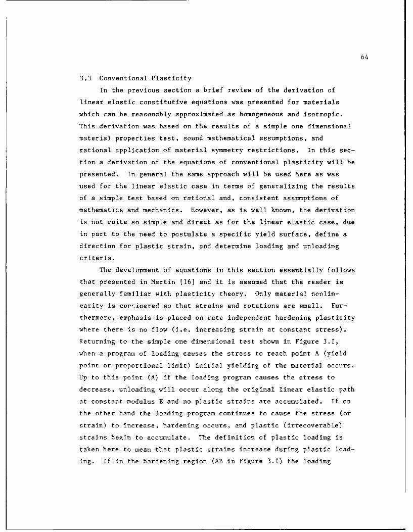
64

3.3 Conventional Plasticity

In the previous section a brief review of the derivation of

linear elastic constitutive equations was presented for materials

which can be reasonably approximated as homogeneous and isotropic.

This derivation was based on the results of a simple one dimensional

material properties test, sound mathematical assumptions, and

rational application of material symmetry restrictions. In this sec-

tion a derivation of the equations of conventional plasticity will be

presented. In general the same approach will be used here as was

used for the linear elastic case in terms of generalizing the results

of a simple test based on rational and, consistent assumptions of

mathematics and mechanics. However, as is well known, the derivation

is not quite so simple and direct as for the linear elastic case, due

in part to the need to postulate a specific yield surface, define a

direction for plastic strain, and determine loading and unloading

criteria.

The development of equations in this section essentially follows

that presented in Martin [161 and it is assumed that the reader is

generally familiar with plasticity theory. Only material nonlin-

earity is cornidered so that strains and rotations are small. Fur-

thermore, emphasis is placed on rate independent hardening plasticity

where there is no flow (i.e. increasing strain at constant stress).

Returning to the simple one dimensional test shown in Figure 3.1,

when a program of loading causes the stress to reach point A (yield

point or proportional limit) initial yielding of the material occurs.

Up to this point (A) if the loading program causes the stress to

decrease, unloading will occur along the original linear elastic path

at constant modulus E and no plastic strains are accumulated. If on

the other hand the loading program continues to cause the stress (or

strain) to increase, hardening occurs, and plastic (irrecoverable)

strains begin to accumulate. The definition of plastic loading is

taken here to mean that plastic strains Increase during plastic load-

ing. If in the hardening region (AB in Figure 3.1) the loading

65

B

A

/

//

//

Loading-unloading response of a hardening material

program begins to cause the stress (strain) to decrease, unloading

occurs along a linear elastic path with modulus E as shown in the

figure above. The material represented by the figure above is

referred to as a hardening material because when unloading occurs

(say at point 1) followed by reloading a linear elastic response is

observed back up to point I where the stress oI is greater than

aA' the initial yield stress. Therefore we might say that the

plastic loading program from A to I hardened (or pushed up) the yield

point of the material from aA to (I I An important feature of the

stress strain response presented is that once the material is

stressed beyond point A, a knowledge of the loading history is

required in order to predict the stress corresponding to a particular

66

strain, or to predict the strain corresponding to a particular

stress. The material is said to be history dependent and a portion

of its plastic loading history must be recorded for reference. If

the material is never stressed beyond point A there is no need to

record the history of loading since elastic response is not history

dependent. By observing the response features in the above figure we

might try to select parameters (hardening parameters) which could be

used to record the history of loading so that given the current

strain we can predict the corresponding stress or vice versa. One

hardening parameter might be a record of the highest previously

attained stress during the program of plastic loading. For example

if the highest recorded stress is 1 1 and the current strain is

FA then the current stress is and the plastic strain is E,A

Another choice of a hardening parameter might be total plastic

pstrain. For example if tie total measured plastic strain is c,

and the current strain is EA then the stress is again calculated as

The concept of yield point (i.e. proportional limit) in the one-

dimensiona] test can be generalized directly to a yield hyper-surface

in stress space. The region bounded by this surface is the elastic

region and when the stress path, corresponding to a loading program,

lies inside this region there is no accumulation of plastic strain.

The hardening concept is generalized by making the yield surface a

function of stress a and parameters H (a = 1,2 ..... n) which

represent a portion of the loading history (recorded history) con-

tributing to taie position of the yield surface and plastic strain.

The initial yield surface is therefore defined as:

F = F (a, H )

Recalling the one-dimensional test, the recorded history parameters

ould be components of plastic strain, measures of work, or some

67

internal variables, because one could derive a simple mathematical

model for this test and successfully predict the results of any load-

ing program as long as the total history of loading (e.g. plastic

strain) is recorded. Figure 3.2 presents the different regions of

stress space and the initial yield surface as discussed above.

/Elasticregion.

Figure 3.2 Yield surface and elastic region in stress space

It is clear that for points inside the yield surface F < 0 , while

for points on the yield surface F = 0 , and for points outside the

vield surface F > 0 . Due to the incremental nature of plasticity

we are int :ested in small changes in stress and strain. If a pro-

gram of loading has resulted in the stress point being on the initial

yield surface then

F (o, H) H =0

c C

If the loading program continues and results in a small change in

stress dc such that the new stress point falls inside the initial

yield surface then

68

3FddF H- 2 do < 0dH Bo ~

and unloading is said to occur. If on the other hand the loading

program continues and results in a change in stress do such that

the new stress point is still on the initial yield surface then

9F do = 0

and neutral loading is said to occur. There is no change in the

recorded history during unloading or neutral loading. Finally, if

the continued loading program results in a small change in stress do

such that the new stress point lies outside the initial yield surface

then

OFdo > 0

and loading is said to occur. It is important to note that we have

defined criteria for unloading, neutral loading, and loading based on

gradients of the yield surface while Ha remains constant. Also, we

observe that stress states outside the yield surface cannot be

obtained unless there is a change in the recorded history Ha

Therefore when loading occurs, Ha must change and we could write

the follow'ng

F(o, Ha) = 0 3.10

and

F(a + do, Ha + d~a) = 0

Equations (3.10) imply

dF = 2 do + dHa = 0 3.113 Ha

69

Equation (3.11) is often referred to as the consistency condition,

and as will be shown later provides for a smooth transition between

loading and unloading conditions. Equations 3.10 and 3.11 play a

very important role in the development of plastic constitutive equa-

tions. Note these equations are differential in form and this must

be kept in mind when incremental solutions of the equations are

sought. Figure 3.3 presents graphically what is taking place in

stress space under a loading increment. As the initial yield surface

is "pushed out" during loading the new yield surface is referred to

as a subsequent yield surface or a loading surface.

I /

Oz,,

Figure 3.3 Subsequent yield or loading surfaces

In order to complete the development of a general plasticity

theory we must determine the functional relationship between the

increment of plastic strain and stress, hardening parameters, and

increments of stress. Since we require that plastic strains do not

increase unless the recorded history increases, it is reasonable to

assume that changes in the recorded history dHc are the result of a

stress increment da and can depend on the current stress a and

recorded history Ha . Therefore, we can write (in index notation)

dep = h. (da, Ha) dHcE 3.12i iO ~

70

This general representation satisfies the requirement that plastic

strains do not accumulate unless the recorded history changes. Also

since we are concerned here with hardening behavior only (i.e. no

flow) no terms can appear in (3.12) which are independent of do and

furthermore since we consider infinitesimal do , terms of second and

higher order in do can be neglected. Therefore we can assume that

dep is homogeneous and degree one in components of do . Recallingi

the one dimensional test, it is reasonable to assume that do con-

trols the magnitude of d-a , which can be argued by considering

equation (3.11) with only I recorded history parameter.

- I F dodH F ,9

Also it can be assumed that the direction of dHa is a function of

, Ha , and not do . Since in the above equations - do is in

effect a dot product or scalar quantity and therefore do contributes

only to the magnitude of dH . Therefore we can express dHa as

dHa b tci (o, Ha) 3.13

where b can be evaluated by substituting (3.13) into the consis-

tency condition. When this result is substituted back in (3.12) we

have

d p =p hia ta 3F doi t 3F 9ok k 3.14

Since we have assumed hia ta and 3F/Ha each depend only on the

state variables a , Ha equation (3.14) can be written

de' = fi(a, Ha) 3k d k

i 3Ok dk

71

since fi(2, Ha) is a vector valued function of a , Ha we can

express this vector as

g(2, 'HO)fi(2, Ha) = G(2, Ha) 3ai 3.15

here G(2, Ha) can be considered a scalar hardening coefficient and

g(2, Ha) can be considered the plastic potential function.

In summary we have generalized the one-dimensional constitutive

equation to predict the hardening plasticity behavior of suitable

materials loaded in three dimensions. At this point it is important

to note that the development of the above constitutive equations was

strongly influenced and probably dominated by observations from tests

on polycrystalline metals and not concrete. The assumption that the

direction of the plastic strain increment should be independent of

the stress increment do is primarily based on conditions required

for the development of a glide-system of crystal grains. Plastic

strains result when such a system is activated, and a certain stress

state is required to develop the system. The required stress state

is a macroscopic stress state which is equivalent to some statistical

average of individual grain shears along critical slip directions.

Once the stress state for the glide system is developed, along with a

preferred direction for plastic strain, the stress increment dc only

contributes to the magnitude of the plastic strain. Based on the

above arguments and the observations that very little plastic volume

change is observed during plastic loading the plastic strain incre-

ment direction is assumed independent of da and the plastic poten-

tial is assumed independent of hydrostatic stress. The assumption of

no plastic volume strain is not appropriate for concrete and the role

of the stress increment in affecting plastic strain direction will be

discussed in Chapter 4. Finally, the basic equations are, in incre-

mental form using index notation:

72

strain decomposition

dci = de + dJ

linear elasticity

d e = Cij oj

where Cij, is the compliance matrix reduced to the isotropic, linear

elastic form with constant coefficients.

yield surface

F O

where the inequality sign is used since we are considering all acces-

sible states of stress. Finally, the plastic strain increment dci

is determined from the following conditions

deJ = 0 for F(a, Ha) < 0 elastic regionI

for F(u, Ha) = 0 unloading

dEP = 0 and - do 5 0 or neutral loading

for F(o, Ha) = 0 loading

dEo = G dok ad-d do 0 oi neutral loadingi G 1 0k c -

The inequalities are included for both unloading and loading condi-

tions due to the consistency condition, which as previously pointed

out provides for a smooth transition between the behavior in loading

and unloading. Change in recorded history

73

dHa - ta Fdota 3F__ k

9B

where ta = ta (a, Ha)

For the case of plastic flow we must allow change in plastic

strains while the stress remains constant. However, this is in con-

flict with our previous assumption that plastic strains cannot occur

as long as the yield surface remains fixed which implies no change in

recorded history parameters Ha . This problem can be resolved by

recognizing that Ha are only part of the total internal parameters

which affect plastic strains. These additional internal parameters

are defined here as JB (B = 1,...m) such that

dep = h. dHa + hj dJB

where hj =hj (oj, Ha, J)

From a computational standpoint flow can be allowed by defining a

maximum strength surface which bounds all loading surfaces. When the

stress point tries to move outside this surface it is forced back by

some return procedure to a new stress point which is still on the

surface and the associated plastic strains are calculated.

Quite often the plastic strain increment is written as

dc p g

where X is a scalar hardening parameter defined as

H FG(2, Ha) do2

74

Recalling the consistency condition (Equation 3.11),

dF = 3- do + L dH = 0

here it is assumed that H is a scalar function of the plastic

strain vector Ep , we can solve for the scalar hardening parameter.

Substituting the expressions

edo E d C

dH =SHde p

3E p~

in the consistency condition results in

3F E (dc -dE) + F 3H d p =0

and since

an expression for the scalar hardening parameter can be obtained as

E de

MI ~p ~oF MH 3gF E 213H Ep ac 3a ~3a

Recalling

do = E d e E (de -dE p )

75

the incremental constitutive equation can be expressed as

cia = 2F EH -a d

3C -

76

3.4 Material Stability Postulates, Uniqueness.

The stability postulates discussed in this chapter are not pre-

sented as thermodynamic or physical requirements of real materials.

These postulates are often used as a basis for developing constitu-

tive equations for certain classes of materials. Returning to the

one dimensional test as shown below, we observe that a monotonic

increase in stress produces a monotonic increase in strain in the

region 0 A B.

B

a2

One-dimensional test results

This can be expressed mathematically as

(2 _ 1 - I 0 3.16

and this inequality can be taken as the meaning of work hardening in

the one dimensional case. The equal sign is provided to allow for

infinite or 0 slope. Equation 3.16 is simply based on the observa-

tion that the assumed homogeneous, isotropic material when subjected

to a one dimensional monotonic increment cf stress responds with a

monctonic increment in strain. Inequality (3.16) can be generalized

to represent multi-dimensional states of stress and strain in the

following way. A monotonic 7hange in a single stress component

results in a straight line path in stress space, and we require the

product of this change in stress with the associated change in strain

to be non-negative, therefore

77

(U 2 2 1 0 3.17(Ki - o.) " (c. - .) - 31

Since an infinitesimal stress increment is applied monotonically and

results in an infinitesimal strain increment inequality (3.17) can be

expressed as

do dc 0 3.18

Another feature of the one dimensional test is that the unloading

slope in the region AB is elastic and this slope is greater than the

slope in the hardening plastic loading region. This feature can be

preserved if it is required that the complementary work around a

closed cycle in stress be non-positive, therefore

c do ! 0 3.19

The equal sign holds for stress cycles in the elastic region. If the

stress cycle produces a change in plastic strain AcP which is

infinitesimal or small, inequality (3.19) is referred to as the

second postulate in the weak form. If no restrictions are placed on

the size of AP inequality (3.19) is referred to as the second

postulate in the strong form. Drucker [17] also identifies work

hardening for the one dimensional tests with monotonic increments in

stress producing monotonic increments in strain. However, in gen-

eralizing this feature Drucker considers the work done by an external

agency which slowly applies load then slowly removes the load. The

external agency is completely independent of the loading program

which produces the existing state of stress and strain in the mate-

rial. Drucker then states that for all sets of added stresses (due

to the external agency) work hardening implies that the material will

remain in equilibrium and:

78

1. The external agency does positive work during the applica-tion of load

do dE > 0

2. The net work performed by the external agency during acycle (application and removal of the load) isnon-negative.

do (dE - dce) = do dcp 0

As previously mentioned, these postulates are not intended to be

physical or thermodynamic requirements for the behavior of real

materials but can be used to develop rational and consistent consti-

tutive relations for broad classes of engineering materials. These

stability postulates prohibit the types of stress strain responses

shown in Figure 3.4.

(a) (b)

/

(c)

Figure 3.4 Examples of response features which violatesstability postulates

Figure 3.4(a) of course is the response featur. referred to as strain

softening and is often observed as shown previously in unconfined and

79

low confinement compression tests on concrete and other materials.

It was reasoned by Ba'ant [10] that strain softening can only be

observed on material test specimen with micro-inhomogeneities. Often

we construct a constitutive model based on a softening stress-strain

curve (actually developed from a force displacement curve) which

assumes homogeneity of stress and strain when significant in homo-

geneities actually occur (eg. cracking, shear bonding, etc.). Con-

stitutive models developed in this way should not be expected to

effectively reproduce material response over a wide range of complex

loading conditions. Therefore, it is expected that some models may

provide good results for specific load cases and be totally inappro-

priate and possibly unstable for other load cases.

The stability postulates presented above are considered as

mathematical restrictions on constitutive relations in plasticity

theory. These restrictions result in the requirement that the yield

surface be convex. At a singular point (corner, vertex) on a yield

surface or at the intersection of two or more surfaces the plastic

strain increment must be within the fan or hypercone bounded by the

normals to the respective surfaces at the singular point. Further-

more, for hardening, satisfying the stability postulates leads to a

sufficient condition for uniqueness of solution in the incremental

sense, where equilibrium equations and kinematic relations are

linear. Since yielding and other nonlinear response features of con-

crete are strongly dependent on the confining stress level, different

forms of loading and failure surfaces are often used for different

stress regions. When these surfaces are combined in a constitutive

model, intersecting corners can occur. If the loading stress path

intersects these surfaces at a corner point, obviously there exist

more than one surface normal at this point ard the direction of

plastic strain is not uniquely defined. Tf the plastic strain incre-

ment at s;uch a singular point, which is the intersection of say m

contiruous yield surfaces, is taken as the linear combination of the

m plastic strain increments for the reacti'e surfaces, then the

80

solution is unique and the stability postulates are satisfied. Here

reactive implies those surfaces which are to be used for computing

plastic strain increments. Proofs of uniqueness can be found in

Martin [16] Pages 109-114.

81

3.5. Examples of Hardening and Softening Formulations.

Consider a homogeneous isotropic material subjected to loading

under plane stress conditions such that 03 = 0. Furthermore, assume

the material behaves the same under tension and compression and that

the Von Mises yield condition is appropriate for describing the ini-

tial yield and subsequent (loading) yield surfaces for the material.

Also, let the one-dimensional response of the material to axial

stress be as shown in Figure 3.5.

Figure 3.5. One dimensional responseof example hardening material

For the Von Mises surface initial yielding will occur when the state

of stress satisfies the condition

2 2 2 3201 + 02 1- 2 = '0 3.20

and for any subsequent yield or loading surface the stress state will

satisfy the condition

2 2 -2F = c1 + 02 -1a2 -G =0 3.21

32

where a = the largest previous value of

12 + 022 - a 1a29 assuming a 0.

Finally, it is assumed that an associative flow rule is appropriate

so that it only remains to determine G (aij, Ha), the scalar

hardening parameter, before stress strain response problems can be

solved. To this end we assume that the hardening is isotropic which

means that G is constant on any particular yield or loading sur-

face. An important result of this assumption is that the hardening

characteristics for the material can be completely determined from

one simple test. With the assumptions made above the basic incre-

mental equations for the case of plane stress are

1(Y v de = dodEe V do de 2 2 V do

1 E E E E 13.22

dep = G 'Y dF , dEP = G 'F dF

1 a1 2

It remains to determine G, which can be accomplished in the fol-

lowing way for isotropic hardening (i.e. G has the same value at

all points on any one subsequent yield or loading surface). Assume

that a monotonic one dimensional compression test is conducted on the

material discussed above such that the stress strain response is as

presented in Figure 3.5. Since the basic equations must apply to

this test and since the loading is monotonic, we can write

dE L 0 o oo

E

and

de dEe + d p 0 > 0o

83

Therefore from equations (3.22) for de,

dol F I'Fde + G 2- - do

d 1 E 3 oI 3a

where here a, = a, and a2 = 0 such that

dE = [ + 402 G] do 3.23

From Figure 3.5 it is seen that the relationship between increments

of stress and strain can also be written as

1

dE = - do 3.24ET

During this monotonic loading condition the stress a continuously

satisfies the yield condition 3.21 so that F = 0 and consequently

a = a. With this in mind Equations 3.23 and 3.24 imply.

G = I -I I 3.254G2 ET E

For this example we are treating compression as positive and only

concerned with the positive quadrant of 0 1G 2 space. From 3.25

G(2, Ha) is a function, of the current stress state (through G) and

could also be expressed as a function of plastic strain P. There-

fore, given Equations 3.22 and 3.25 we can solve hardening plasticity

problems under monotonic loading given a particular stress path in

plane stress space (0102). From Figure 3.5 we can write Et (u) so

that the integration of Equations 3.22 could be performed with rela-

tive ease. For a particular continuous proportional loading path

(say Gi = 20,) the effect on the loading surfaces is uniform

84

expansion as shown in Figure 3.6. The reason for this is that as

loading progresses a increases and G is always positive since

E <E.t

Figure 3.6 Isotropic hardening of yield surfaces

Based on the above assumptions the exact solution to the problem of

continuous proportional loading (doI = 2do 2) to a final stress state

a = 2c0 can be obtained. For this example we take the case where

E = constant.t

At the end of the elastic region (ie; a1 = o, 02 = r o) the elastic

strains are calculated from (3.22) as

e1 r G (2-v)

e r Go(0 v2 - 3E (1-2v)

For the remainder of the stress path, the total strains can be deter-

mined by integration as

a

85

- 63450 E - EToo -(2-v) + E"E -E T

E2 = 2 (1-2v)2 2E

The main point to be made here is that for hardening plasticity the

solution to this simple problem can be obtained in closed form.

If on the other hand, the one-dimensional response to axial loading

is observed to be that presented in Figure 3.7 several different

problems arise in obtaining the solution of the plane-stress problem.

E.

ell

Figure 3.7. One dimensional response ofexample softening material

Here it is assumed that the softening behavior observed in the

one dimensional test (Figure 3.7) is generalized to an isotropic

softening in plane-stress space. The qualitative effect of the

softening on subsequent yield surfaces is shown in Figure 3.8. Since

the increment in stress do for

86

0*2

GS

G/-

Figure 3.8 Isotropic softening of yield surfaces

plastic loading in the softening region will be negative our previ-

ously defined loading and unloading criteria will not be appropriate.

Also, since plastic loading continues as a and therefore-2

decrease, the largest previously attained value of o cannot be

used as a recorded history parameter. Furthermore, we cannot use the

smallest previously obtained value of a since a decreases under

elastic unloading also. Therefore it appears that plastic loading

should be defined here as increase in plastic strain. Another prob-

lem encountered in softening materials is demonstrated in the figure

on the following page.

For stress space plasticity, a is the independent variable and

strains are solved for from the equation

a p

87

I / I

//

/ B /A B A

E B Er

E

/

Hardening material. Softening material.

while for strain space plasticity c is the independent variable and

stresses are solved for from the equation

a = E c - cR

where cR is a stress relaxation from the stress which would be pre-

dicted under purely elastic response. For the softening problem,

conceptually, some inconsistencies are indicated by the stress space

formulation. First the end point (cB ' aB) cannot be reached by fol-

lowing a monotonic load path and since the strain must be specified

in this test we do not know a priori what the final stress aB will

be. The stress space formulation could be used foi the isotropic

softening problem by developing a softening function G in the fol-

lowing way. Specializing Equations 3.22 to the softening material

shown above following the same procedures used for the hardening

material results in

88

4-2 [E T E

Therefore considering only the plastic strain components for the2. 2 =-2

plane stress problem (where F = o 0 2 - 1Ia2 = 02) we have

dE = + 2a (20i do4 + 2c. do1 402 LET E] 1 1

and

Sp=L+ 2a, (2G I do, + 2 d4 -2 E - 2 2

Here again the problem is we do not know the stress path as a func-

tion of strain in the plastic region and we cannot obtain a general

closed form solution as we'did in the case of the hardening material

using a stress space formulation. For the special case of an iso-

tropic material and a symmetric-monotonic plastic loading path (ie ElP P

= £2) to a final plastic strain state of EI =2 = C a solution

for the softening material problem can be obtained. For this case

a, = 02 , and -do -do2 due to symmetry. Therefore from the above

equations

0p I = (

£0 10 E1I T Cu

and

I Io A1~ 0~ (1+! T -C

from which the final stress u can be solved for. The point to be

made here is that an additional assumption (symmetry) had to be made

before this simple problem could be solved.

89

3.6 Fracture Energy Based Model

3.6.1 General

The Fracture Energy Based Model (FEBM) was developed at the Uni-

versity of Colorado (3) in an effort to provide a rational and

consistent formulation for predicting the triaxial response charac-

teristics of plain concrete to include strain softening. The model

is based on conventional plasticity in the sense that it makes use of

initial yield and loading surfaces, decomposition of strain incre-

ments into elastic and plastic components, a flow rule, and the con-

sistency condition. The loading surfaces expand with increasing

plastic strain and hydrostatic compressive stress and rotate about a

point of equal tension stress. The model is developed for both asso-

ciated and nonassociated flow assumptions. The strain softening

formulation is based on fracture energy concepts and the criterion

that strain softening occurs when the loading stress state reaches

the failure surface at a confining stress less than the confining

stress which defines the brittle-ductile transition.

3.6.2 Failure Surface

The failure surface used in the FEBM was developed by Leon (18),

and is based on forcing continuity between the Mohr-Coulomb friction

law and the tension cut off condition of Rankine. Mathematically the

two parameter surface is represented as

F 1 3 + Mo 1 - C = 0 3.28C c

where = Major principal stress

li = Minor principal stress

Mo = friction parameter

C = cohesive parameter.

f'= Unconfined Compressive StrengthC

90

When 01 = 0 equation 3.28 yields

03= Cof,

2

C

so that taking 03 = fc for this case results in C = 1 . This is0

the same result found for the Mohr-Coulomb surface where C would0

be defined as the normalized cohesion of the material while the fric-

tion parameter Mo is not exactly the same as the coefficient of

internal friction, which is defined in the Mohr-Coulomb model, it is

a measure of the slope of the failure surface (and loading surfaces

to be discussed in the next section).

The failure surface defined by Equation (3.28) and shown .n Fig-

ure 3.9 represents the maximum strength of the material when the nor-

malized cohesive

Maximum strength. k=1.0k=.9

k=.2

Figure 3.9 Hardening and maximum strength surfaces for the FEBM

91

parameter C = 1. Mo can be determined by setting 03 = 0 and defin-

ing the "alue of o for this condition as 01 = f' which leads tot

f2 _ f

2

c tMo - c 3.29f, f,

c t

where f' = unconfined tensile strengtht

3.6.3 Loading Surfaces (Hardening)

The loading surfaces for the FEBM during hardening can be

expressed as

012 I - 3 k2 01F (o, c, k) = (I - k) - + f, + Mo - ko2 3.30

C =00

where k (cp) = hardening parameter, ko ! k I

k = value of k defining the initial yield surface

Loading surfaces for different values of k are presented in Fig-

ure 3.9. Three important observations can be made regarding the

loading surfaces.

1. When k = I the loading surface corresponds to the failuresurface F.

2. The hardening behavior is not purely isotropic, since theloading surfaces essentially rotate about a common point inthe tension region.

3. The loading surfaces intersect the hydrostat at angles otherthan 90' and other corners exists at 60' intervals in devia-toric sections.

In order to simulate the pressure sensitive behavior of concrete the

hardening parameter is expressed as a function of plastic strain and

92

confining stress. The development of the expression for k was

motivated by the fact that increasing the confining stress (o = a2)

increases the maximum strength (03) and the strain (c3) at which

maximum strength is reached. Therefore, one could conduct tests at

low, medium, and high confining stresses then normalize the ordinate

(i.e. a3(EP)/3max = k) and plot k versus plastic strain (cp) up to

strains where maximum strength is attained. The general characteris-

tics of these curves are shown in Figure 3.1C. To simulate this

variation of k with J, a monotonically increasing elliptic function

of £p was selected.

(0P, XP) = ko + 1 - ko -2 p p ( p) 2 3.31cp

where x- ductility parameter, the plastic strain when maximum

strength is attained for a given confining stress.

ip •P = equivalent plastic strain rate.

An empirical expression was developed for XP which is also calibrated

from low, medium, and high corfining stress test results. This

expression is

X () ( + BH + CH 3.32

ideally for a given concrete three triaxial compression tests can be

conducted (eg. low, medium, high confining stress (ai)) and three

values of xP , measured. Then knowing f' and a these equationsC I1

in the unknowns A', BH , and CH can be determined, and solved.

93

confinement, confinement.

k~l

kk

x "(a-)

Figure 3.10 Effects of confining stress on hardening param~eter k

94

3.6.4 Loading Surfaces (Softening)

If the loading stress path intersects the failure surface (Equa-

tion 3.28) below the brittle-ductile transition point (TP) and load-

ing continues (i.e. AEP > 0) strain softening is predicted by the

FEBM. This softening response is accomplished by collapsing the

failure surface through a continuouS decrease of the cohesive parame-

ter until a residual strength surface is reached. The initial and

residual strength failure surfaces are presented in Figure 3.11. The

cohesion is decreased according to the expression

- ctf?

t f 5 3.33

at fV e (~t Ur!

where

f' = tensile strength of concretetot = degrading tensile strength

Uf = crack opening displacement measured in a direct ten-sion test

Ur = residual crack opening displacement, crack opening atfracture.

As shown in Figure 3.11 the decrease in cohesion is accompanied by an

increase in M (the frictional parameter) or say a frictional harden-

ing. In effect the softening surfaces rotate about the point TP in

stress space. The relation between M and C is assumed as

M = M - (M - Mo) C 3.34r r

Where M is the value of the frictional parameter at residualr

strength. The cohesion parameter C can therefore be thought of as

the softening parameter and can be determined from a simple uniaxial

tension test (which is conducted in stroke control). The results

95

/k=l.Maximum _

strength.Transition point.

Residualstrength.

//

Figure 3.11 Rotation of softening surfaces about TP

from a direct tension test along with predictions from equation 3.33

are presented in Figure 3.12, (from Reference 3). The motivation for

using the direct tension test for defining softening in compressive

stress states, was based on the idea that the strain softening phe-

nomenon is dominated by microcrack growth which is associated with

dilation (expansion) in compressive tests. Considering the case of

direct tension a strain softening plasticity fermulation can be

developed in the same manner as for hardening plasticity. Assuming

the initial yield and loading surfaces can be defined by the maximum

tension strength surface

96

1.0 A,

0 Experimental Data

.75 at -f

.50

0

Ed

.25

0.0 .25 .50 .75 U1 1.0Ur

Figure 3.12 Softening in a direct tension test

F(aI, t) = aI - at = 0

where at = Ct (Ef)

Ef = fracture strain

and that the plastic (fracture) strain in tension Is defined in rate

form as

BF

-f f a

where

f c d

97

the consistency condition is given by

DFtE 2F) LO-t Lef t 2*

F t E - 3.35

__ C

f Ta F t

E + (3F E 3F

where the softening modulus E is defined as

ft

E = ( Ef 3F 3.36f 3-f

Up to this point basic concepts of plasticity (i.e. strain rate

decomposition, normality, consistency) have been applied to a strain

softening material. However, when attempting to compute Ef from

Equation (3.36) a problem arises due to the fact that at is defined

as a function of Uf not Cf (Equation 3.33, Figure 3.12). The reason

for this is that in a direct tension test (in displacement control)

at peak stress the microcracks coalesce into a localized band and the

response of the specimen is better or more appropriately defined in

terms of stress versus displacement (crack opening displacement) as

shown in Figure 3.13 (from Reference 3). In the FEBM this problem is

addressed by using the chain rule such that

90t 9at 3Uf

3Ef TUf af

Thprefore, the softening modulus can be expressed as

E Ot uf 3Cf F37

f = Cf Ef -;f -3

98

and the only term which c:nnot be directly computed is 3U f/36f It

i, here where an assumptiorn is made which will allow for the exten-

s i'on of the strain

T a

Ed

'uf Uf

Composite Crack and Element

ef ef

]. vl

I-b

,: quivalent Jontinuum:

Figure 3.13 Local.zation versus continuum ideas, from (3)

softening theory to compressive F ress states but also results in a

theory which when implemented in finite element analysis procedure

will exhibit mesh sensitivity. F sentially this assumption is to

smear the effect of the localizee crack band over the volume of the

test specimen. This is accomplished by expressing the softening mod-

ulus (for the direct tension test as

E E hf d t

99

where Ed = 9C aTUf

ht = aUff sf , height of test specimen.

t( f \\"f f

For the direct tension test ht can a so be expressed as the elemer-

tary volume of the test specirien div ded by the cracked surface at ea.

Vt A

The theory is ext aded to comp essivw stress states directly by using

the failure surfa, 2 in the pos peak region

\l - 02 1F f, M fl03- C = 0

c / C

where C and M ire defined by Equations (3.33) and (3.34), -.spec-

tively. Also, in 'he softening region the equivalent plastic rac-

ture) strain increment is determined from

t;f < Cf f ~~

tere the McCiuley brackets <> extract only the positive com-,onents

nsion) of .ie inelastic fracture strain rate tensor ;f . he

,-y question remaining for the compressive formulation is how to

_ termine DUf, af for compressive stress states. Here, a similar

ument as u ed previously for the case of direct tension is pre-

t ited. The ssumption is m,:de that under compressive 3tates an

e aivalent ch.racteristic lei gth can be defined such that

100

Uf V-_ = hc

(Ine might think ot the volume fraction Ac/V as microcrack density incompression. While it was quite clear how to determine A in the

t

tension test it is not so obvious how Ac (the fracture surface

area) should be determined for low confinement compression tests.

Under unconfined and very low confinement compression tests, vertical

(splitting tensile) cracks form which are the result of mode I type

fracture (ie fracture due to tension only) in the circurnferpnrial

direction. Tf the area of these vertical cracks, which ale the

result of splitting compression, is defined as Ac then the fracture

energy associated with this fracture can be expressed as

z = C Ics f

When tesults of compressive splitting tests are compared to direct

tension tests (see Figure 3.14) it is seen that the fracture energy

reiease rates in tension and splitting compression are quite similar.

As the confining stress is increased the tensile cracks tend to

coalesce into a single shear band which is inclined to the vertical

axis of the specimen. The area of this shear fracture surface AAs

is of the same order of magnitude as PAt and this type fracture is

essentially mode !T (ie fracture due to shear). The energy associ-

ated with this fracture can be expressed as

II= I1r, =II AA 'C AAt

cv Gf s f t

By equating the energy in -ompressive splitting tests to that in com-

pressive shear an approximate Ppresion can he determined for AAc

11

MAc = " tAGf t

10l

Figure 3.14 Comparison of softening in tension and compression

and therefore

I

h Cf hc Gf11 t

where h there is the height of the test specimen. From test

results it was determined that the ratio G /1 G increases rapidlyf f

with confinir.g stress and the following empirical formula was

developed.

IGC

•s - ? -

fC

1 ,5

G

102

where As and Bs are determined (in a manner similar to that dis-

cussed for the hardening coefficients A, Bh and Ch) based on low

and high confining stress tests.

3.6.5 Non-Associated Flow

As pointed out in previous discussions constitutive equations

based on associated flow plasticity which do not incorporate a plas-

tic volume change tend to overpredict lateral strains or dilatancy.

This of course is due to the fact that in general these models make

use of the normality principle for plastic strain direction while the

effects of the hydrostatic component of the stress increment is

ignored. To reduce this predicted dilatancy a plastic potential

function not equal to the yield surface can be used. The main prob-

lem here is that this produces a non-symmetric material stiffness

matrix which leads to increased computational time. It seems reason-

able to assume a plastic potential function that is similar in form

to experimentally verified yield and loading surfaces and also is

consistent, in terms of predicted lateral strains, with test results.

For the FEBM non-associated flow is characterized by a plastic

potential function (Q) which is not equal to the loading surface F.

The plastic potential for non-associated flow hardening response is

defined as.

al ( a 1 3 2 MQ k2

Q(aI' 8' k, M) - 1 +- ( 0 + k k C = 0 3.38

cc c

and for softening response

Q(ol, o3, k, MQ) ( f3) + f - C = 0 3.39

103

From equations (3.38) and (3.39) it can be seen that the only differ-

ences in the plastic potential and the loading surfaces (i.e. equa-

tion (3.30) is in the modification of the friction parameter M + MQ.

The parameter MQ is referred to as the dilatancy function since it

primarily controls the amount of dilatancy. For non-associated flow

the gradient of the plastic potential defines the direction of the

plastic strain increment as

p c

where

2Q Q S1 [ 0

3Q I - Sh

S(3

where

, +a I- a1 c1 - 3

S = 2 [(1 k) f] fc

From the above it can be seen that 3MQ is a measure of the lateral3o1

component of the plastic strain.vector and can be determined from

triaxial compression tests at different confining stress levels.

Essentially MQ is determined from three tests, unconfined tension,

low confined compression and moderate confined compression. An

iterative procedure was used to select MQ to best fit the experi-

mental data. It was found that an empirical relation for MQ as a

function of aI could be determined as

M = D /-0\lI f) - E /I l -\/4f)/ + FG

104

3.7 Endochronic Plasticity Model

3.7.1 Background

The first endochronic plasticity theory was proposed by

Valanis (19) in 1971 and was based on the principle that the history

of deformation of a material could be defined in terms of a "time

scale" which is not real time but is a property of the material. The

time scale is assumed to be a monotonically increasing function of

the total deformation of the material and is essentially a metric of

the deformation path in strain space. Also, the theory does not

depend on the notion of a yield surface and definitions of loading,

unloading, or reloading criteria as is the case of conventional plas-

ticity. The first theory attracted considerable review, and discus-

sion in the engineering community. Probably the most prominent

criticisms of the theory were presented by Sandler (20) and

Fivlin (21). Sandler's criticism was based on the fact that the

theory fails to predict closed hysteresis loops during unloading and

reloading of a simple endochronic material. Sandler then showed

where this problem could lead to numerical instability and non-

uniqueness of solution. Rivlin carefully analyzed the feasibility

and plausibility of using the endochronic theory to model materials

in general. Rivlin was also critical of the thermodynamic arguments

used in the development of the theory. The problem of hysteresis

loop closure was addressed by Valanis (22) and formed the basis of

the new endochronic theory for concrete which is discussed in Sec-

tion 3.6.3. A key feature of the new endochronic theory is that the

time scale (intrinsic time) is assumed to be a monotonically

increasing function of the plastic strain increment. A detailed dis-

cussion of the derivation of the new endochronic theory is presented

by Valanis and Read (4).

105

3.7.2 The First Endochronic Theory (Simple Model)

Consider a one-dimensional test of a material which is linear in

stress versus strain and whose deformation is also a function of

time. When an axial stress, which is a function of time, is applied

to the material, the strain is a function of the total history of

loading up to the present time. If the program of loading, here

c(t) , is continuous and differentiable then in a small interval ofdo

time dt the stress changes by - dt this change in stress

results in a change in strain de and the relationship between these

changes in stress and strain during this short interval in time is

dc(t) = C(t-T) do(t) d- 3.40dt

The total strain at time (t) is then

E(t) = t C(t-) da(t) dr 3.41dt

0

A material whose response can be reasonably approximated by (3.41)

can be referred to as a linear hereditary material. If in reverse we

consider a program of straining which results in a change in stress

we obtain a relationship

tk(t-T) dc(t) dT 3.42

(t) f k ) dt

0

The functions c(t) and k(t) are referred to as the creep function

and relaxation function respectively and are properties of the mate-

rial. C(t) can be thought of as the strain produced by a suddenly

applied constant stress of unit magnitude, while k(t) represents

the stress required to produce and maintain a constant strain of unit

106

magnittde. Linear hereditary material behavior can be approximated

using a Maxwell model which is presented in the Figure below.

k c

E S vEd

Maxwell Model

The change in strain for a differential change in time for the model

is

d- de + ded

and since

= E s Ccs d

Therefore

£ -+ -3.43

s E C

When a Maxwell model is subjected to a suddenly applied constant

strain c , and the corresponding value of stress is a equationo 0

(3.43) can be integrated subject to these initial conditions to

obtain

-Etc -Et/ca(t) = a e E E 0 e 3.44

107

This defines the relaxation function for a Maxwell model. The rate

of stress change is

o~t o) -Etfc

so that the initial rate (i.e. at t = 0 + ) is

Ec

C

The relaxation time is defined as the time for the stress to relax to

zero if the relaxation rate continued at (;(t = 0 ) . Under these

these conditions the equation for stress relaxation is easily deter-

mined from the figure below

tR t

Stress relaxation in Maxwell Model

Therefore tR is determined as

CtR

108

and is a property of the material. Equation (3.43) can be rewritten

as

=E dc+ U 3.45dt Edt EtR

or

de + dt 3.46E EtR

If now we wish to use equation (3.46) to model static loading of a

rate independent material, the time scale is unimportant and we could

define another measure of time, (i.e. intrinsic time) C such that

the differential of intrinsic time could be written

d = Idej

Replacing dt in (3.46) with dC

do + o dcj 3.47E - Et--d

TtR

This is the simplest endochronic model and is the form of the first

endochronic model proposed by Valanis. From (3.47) it is seen that

for loading dc > 0 therefore

do > 0 = E (I - o/EtR) = EL

while for unloading de < 0 and

do d< 0 =+E (+ Et) = Eu

C I dc < 0 =

109

so that for a > 0 and large enough EtR

0 < E.L < Eu

This formuaiaion leads to a response as shown belcw and clearly vio-

lates Drucker's stability postulate for an unload reload cycle of

stress. This problem was alleviated by Valanis [22] by introducing a

new intrinsic time measure which will be discussed in Section 3.6.3.

Ur

Unload-reload for first endochronic model

110

3.7.3 The New Endochronic Theory

3.7.3.1 Basic Equations

As mentioned previously the endochronic theory is based on the

hypothesis that the current state of stress in a material is a linear

functional of the entire history of deformation where the history is

defined with respect to an rtrinsic time which is a function of the

plastic strain increment. The foundation of the theory is based on

the theory of irreversible thermodynamics of internal variables, the

derivation of some of the equations of the theory will be presented

in this section.

For the development of the small deformation isotropic theory it

is assumed that internal dissipative mechanisms can be represented by

internal variables qr (second order tensors, representing devia-

toric mechanisms) and pr (scalars, representing hydrostatic

mechanisms). Furthermore, there exists a free energy of deformation

function P which is quadratic in terms of the strain tensor and

internal variables. Therefore ' can be represented as

= + H

where

D qr)

% (c, pr)

The function ' can be further decompcsed into elastic 'e and

plastic rP parts such that

'P= P (EP, pr)H H

The thermodynamic relations for the plastic parts of the constitutive

equations are.

S4pS D

~ e p

H-P

Due to the assumptions made for 4 (ie isotropy, quadratic in strain

and interne! :ariables) it can be reduced to the canonical forms

P 2 p I J p - r 22 r

and 3.48

1 K r(E p - pr)H 2f r

A simple one dimensional model of an endochronic material is pre-

sented on the following page.

The force in each spring is

gr = vir (eP - qr)

and the contribution to the free energy of endochronic element

r is

r 1 2

1r (e - r)2

and therefore

r

112

S

One-dimensional model with several endochronic elements

also

pr (p -Or) =gr S3ep r r

and

_r (ep -r) = r

Similar equations can be written for the hydrostatic part. Qr and

Pr are internal stress type quantities and Sr and pr internal

strain type quantities with the characteristics that they cannot be

measured as we normally measure stress or strain. Since the entropy

for the system must be increasing

113

- r dqr > 0 jjdqrjj > 0

p dpr > 0 dprj > 0

and therefore expressing dqr , and dpr , in rate forms we have.

-Qr qr >0

- Pr *pr > 0

For irreversible thermodynamics it is usually assumed that consti-

tutive equations give the forces (stresses) as functions of the

fluxes (strains) or vice versa. This assumption can be expressed as

(1) r

Qr =br qr

No sum on r

Pr = br(2 ) pr

In these expressions br (I ) and br (2 ) play the same role that the

scalar shear and bulk moduli play in relating elastic deviatoric

stresses to deviatoric strains and hydrostatic stresses to volumetric

strains.

From the previous expressions for Qr and Pr the "evolution" equa-

tions are developed as

S + br(1) r = 0

+ br (2)r =

3pr

114

Finally, recalling Equation 3.48.

1ir Sr + br (I ) ir = pr ep

and

kr pr + br(2) pr = kr cp

or

r dr r deP

br(I) gr + d-t dt

and

Kr dpT Pr+ P = K I

(2) dt dt

For a rate independent material the independent variable in the above

equation does not have to be real time, but must only be a monotoni-

cally increasing parameter which effectively records the history of

loading of the material.

For the endochronic theory a parameter is chosen and defined as

intrinsic time (Z) which is a function of plastic strain.

Replacing dt with dz the evolution equations become

r dQr dep

br(1 ) gr + d-zs Pr dzs

and

Kr Pr + dr d P(2) dz dz

br H

These equations ran he solved llqfncy Laplace Transform techniques with

Z as the independent variable. This procedure for the deviatoric

115

evolution equation is presented here. First the Laplace transform of

each term is taken.

Qr j L V I = L dei

L I (I -I)~1 *- qd dz

Therefore defining ar = r

br(1 )

ar Qr (s) + s Qr(s) - Qr(o) = urs eP(s) - vreP(o)

and

eP(o) = 0

Which can be rearranged to express Qr(s) in terms of eP(s)

Q r(o)Or(s) = Qro - 15ers(a + s) + pr + s) s eP(s)

Taking the inverse transform of this equation, and observing that the

second term is the product of two transforms and therefore its

inverse is a convolution integral

-a r z s -ccr (z - z) -de

Qr = Qr(o) exp s + wr exp s dz

0

and similarly for the hydrostatic part.

-AXr z cz H - r (z -7') depFr= Pr(o) e H + Kr i e dz dz'

0

where Xr = Kr

br(2 )

116

Finally since

s = r and a = - Prr r

z dep-ar z s; ~S( r(o) e s + p(z - z') -d., dz'

r s S-o

and 3 .48a

-Xr z + zl, !

0 Pr(o) e s +! z (z H -z) d dz'0

where-(ir z

P Or e Sr

X, r e rzHr

Equations (3.48a) are the general constitutive equations for the

endochronic theory. It is important to note here that the develop-

ment of the endochronic constitutive equations follows accepted

conventional procedures and the concept of intrinsic time or pseudo

time is not new (e.g. viscoelasticity applications). Furthermore,

the exponential forms in 3.48a result from direct application of

applied mathematics principles and not from arbitrary assumptions or

curve fits of experimental data. The basic equations of the new

endochronlc plasticity theory can be expressed as

z dep

s = -(z - z ) dz' 3.49

dzp0 = j7,z ! (zt -Z) drz dz' 3.50

dsdep de - 3.51

drp = df -10 3.52k

117

d p P 2 tnp2 3.53

= dz dz = dz 3.56ds T IF ' dz kF 35S -

where S- = Deviatoric stress tensor.

a = Hydrostatic stress.

( )P = Denotes plastic components.

V = Elastic shear modulus.

K = Elastic bulk modulus.

F = Shear hardening parameter.s

FH = Hydrostatic hardening parameter.

Z = Intrinsic time scale.

Z = Intrinsic time for shear response.s

ZH = Intrinsic time for hydrostatic response.

k = A constant which determines the magnitude of shearvolumetric coupling

Q(z), (z) = Weakly singular kernel functions such that

p(O) = D(O) =

but p(z) and D(z) are integrable

in the domain 0 Z < -

Intrinsic time is analogous to recorded history parameters used in

conventional plasticity. The form of dz in Equation (3.53) was

developed based on the idea that the intrilsic time increment is

given by the increment of the plastic strain path in plastic strain

space and therefore could be written in general as

dz' = P d, dFl 3."7/ijkl ij ~kl

where the metric P is a fourth order, isotropic tensor with th,

general representation

P ~k2 6,j6k +K235ijkl 1 ij k] 2 Ik jl

118

Combining 3.57 and 3.58

dz2 k2 dE dep + k2 dc_ dcd i kk 2 kj kj

or

dz2 k 2 ldePJ 2 + k' HdcP ! 3.59k1 2 [I ll3 5

which is equivalent to Equation (3.53) to within an immaterial multi-

plicative constant. The requirement that p(z) and ?(z) in Equa-

tions 3.49 and 3.50 be weakly singular kernels, essentially comes

from the need for the new model to predict closed hysteresis loops

under unloading - reloading cycles (this was a major problem with the

first model). This idea is demonstrated in the following example.

Consider a typical plot of simple shear stress S versus shear

strain y as shown in Figure 3.15. It is assumed in this figure

that a yield point exists but that the slope of the stress strain

curve is continuous throughout. If we wish to plot shear stress

versus plastic shear strain yp , as shown in Figure 3.15, the S,y

axes can be rotated as shown and the slope of the curv at yp = 0

will be infinite.

The endochronic theory for this case will yield

fZr -z') -- ydz'

s = Pdz'0

Therefore

ds = p(zs -z)

dy YP = 0

which requires p(0) =

119

The series expansion for p

-ar zp r e sr

satisfies the requirement p(O) =

S//

Figure 3.15 Simple shear stress-strain response features

The parameters which must be calibrated in the theory can be

divided into three groups: parameters which describe pure hydro-

static response, parameters which describe the shear volumetric

coupling, and those parameters which describe the deviatoric (shear)

response. The calibration of these parameters will be discussed in

the following sections.

3.7.3.2 Hydrostatic Response

Typical response features of concrete to pure hydrostatic stress

were discussed in Chapter 2. The endochronic functions (ZH) and

F H must be defined and calibrated to capture these key hydrostatic

120

stress-volumetric strain features of the concrete in the stress range

of interest for a particular problem. Assuming that the reference

state is the natural state then under monotonic pure hydrostatic

loading conditions the following basic equations apply:

fz H - z'o ,z )' dz d z

0

dz2 = k

2 tdeP 2

dz dzH kF

From the latter two of these equations it is seen that

k2 IdeP1 2 = k2 F 2 dz

or

dep

d H FH

therefore

a -(z ) FH (P) dz' 3.60

Equation 3.60 provides the functional form to be used for calibrating

¢ and F H to predict general hydrostatic response features. A typi-

cal hydrostatic stress strain curve is presented in Figure 3.16. The

effect of the hardening function FH is best seen in this figure

where a hardening function FH = 1 leads to plastic flow at a stress

CO It is assumed that the general form of F H should be

FEPFH=e

121

,I I

Figure 3.16 Hydrostatic stress-strain response feature

then expressing eBEp in a power series expansion and only retaining

linear terms we have

FH = I + $Ep

From Equations 3.53 and 3.56 it is easily shown that (since for

hydrostatic response dep = dz = ) .

d H dcp d p

dH =FH I + B~p

which upon integration leaves

I PzH = B n( + p

122

therefore

e H = I + 6Ep - FH

Also it is noticed that pure hydrostatic response is independent of

k. Therefore the constitutive equation for hydrostatic response

becomes

j Y H Kr eAr (Z H - e dz'

r f0

or upon integration

K-Xr zH I+ [e(Xr' + 6)zRO ZKr eHr

Where r represents the number of internal variables Kr x r (or

the number of endochronic elements in parallel) required to simulate

the hydrostatic response to the desired level of accuracy. Therefore

there are three parameters Kr P xr X and 6 which must be deter-

mined based on pure hydrostatic test results.

The calibration of the parameters Kr , Xr , and 6 is accom-

plished by first defining a stress o* such that

F H I + BEp

and since for the hydrostatic test p z- and if we assume I +

6c = e we have

a*Kr -(6+ Xr) z Hr ( + xr)

so the two curves of Figure 3.16 can now be used. 6 is determined

from the straight line portion of the second branch of the hydrostat

from the requirement that

123

= a (I + BEP)0

1

Next a plot is made of (a - a*) versus ZH (here ZR I In (I +0 H

BeP)) based on hydrostatic data (note R is known) and values of Kr

and 1 are selected which give the desired fit to this curve.r

124

3.7.3.3 Shear Response.

The shear response is defined by Equations 3.49, 3.53, and 3.56

which require determination of the response functions p(Zs) and Fs

along with the coupling constant k. As discussed in Chapter 2 the

hardening characteristics of concrete in shear are very sensitive to

the confining stress level, also this hardening is dependent on the

direction of loading in the deviatoric plane which can be defined by

the similarity angle 0 . Therefore it is assumed that

F = F (o,O)5 5

and F can be determined from a series of hydrostatic pure devia-5

toric tests as discussed in Chapter 2. The simplest and most direct

way to determine the shear parameters is from a triaxial test in the

IT plane (ie shear under zero hydrostatic stress). However, there

were no tests performed like this for the concretes reported herein

and therefore hydrostatic pure deviatoric test results must be used.

Changes in hydrostatic plastic strain eP due to increments of shear

stress result due to change in Z as defined in Equation (3.53) and

the corresponding change in ZH from Equation 3.56. If the kernel

(ZH) in Equation 3.50 is approximated with a Dirac 6 function

P(z H ) = Ko 6(ZH)

Equation 3.50 results in

dep

= K • - 3.61o dzH

and for pure hydrostatic loading

a = K (I + Ep ) 3.620

Therefore Equation (3.62) is essentially a linear hardening model.

Equation 3.62 seems reasonable especially for the initial portion of

125

the hydrostat (ie prior to signs of locking up) and if aI is the

mean stress during a pure deviatoric load increment we can write

a I

d kp = - dzH 3.63

Therefore as dZH increases due to application of pure shear incre-

ments, due to equations 3.53 and 3.56, dEp will increase as defined

by Equation 3.63. Defining the intrinsic time dZ in terms of a

parameter di such that

ds = jHdcPj , d H = IdePi

a differential relationship between d s and dy can be derived,

where dy is the change in the intrinsic time in addition to the

change caused by pure hydrostatic loading. This expression is

ds [ 2ay 1 3.64

dy - + 2ay

where

k0

a ko1

and

y = Z-Z1 , Z1 is the value of Z at the completion

of the pure hydrostatic branch of loading.

Equation 3.64 can be integrated to give

s x - - log x + - 1) 3.65

126

KB

where X = I + 0 H , 8 is the hydrostatic strain caused by

shear loading at constant pressure.

Finally if W is defined as the increase in Z after the5

hydrostatic loading such that.

W =Z -ZIs s

a differential relation between d and dW can be determined as5

d I 2aFsW 366

dW Fs + 2aFsWJ ]3"

which governs d during loading in a deviatoric section afters

hydrostatic loading. Since

F = F (o,0)5 5

F will remain constant during loading in a deviatoric section ats

constant 0. Finally for this type of loading Equation (3.49) can be

written for a pure shear path as

T f p(W W1 ) dY-P dW10 dW I

and

_F F_2aF W1 1 3.67T = - l p(W - L +: 2r W dW

0'S

127

Valanis (20, in an appendix) shows that

F2aF z'li f Z (z - z') s ]rz -1 + 2aF z' dz' = Mw

z - O L s

where

M (v/'y p) = f o(z') dz'0

and

MO = M(CO) <

therefore the shear stress behaves asymtotically to values T- at

different levels of mean stress and can be written

Fs CO Mw

and the form of F can be determined by comparing r- at differents

mean stress levels.

S ( a)= F

The functional form of P is determined by solving Equation (3.67)

numerically knowing T and a (from experiments).

128

Chapter 4

Comparison of Model Predictions %ersus Test Results

4.1 General

The Fracture Energy Based Model (FEBM) and the Endochronic Con-

crete Plasticity Model (ECPM) are calibrated for the concrete materi-

als used in the verification tests, and stress strain response

predictions are discussed and compared with test results in this

chapter. The concept and operational details of the WES Constitutive

Driver (WCD), which is used in this study, is discussed in Sec-

tion 4.2. Calibration of the constitutive models and an analysis of

predicted and measured results are presented in section 4.3 WES

Tests, 4.4 Colorado Tests and 4.5 Eindhoven Tests. Most emphasis is

placed on comparisons for the WES Tests, because a more extensive

calibration test program was conducted at WES for the f = 6.5 ksicconcrete. In essence a calibration parameter sensitivity study is

presented in this chapter. The objective of this sensitivity study

is not to optimize the values of calibration parameters but rather to

discuss the consistency between parameter values determined from a

calibration tests and those values of the parameters required for

better model predictions.

4.2 WES-Constitutive Driver

The original concept for the WES Constitutive Driver (WESCD) was

based on the need to develop a consistent method to better evaluate

predictions from large scale dynamic finite-element codes. As dis-

cussed in section 1.1, the effectiveness and efficiency o- the con-

stitutive model was obscured by the overall size and complexity of

these large scale problems. Therefore, the concept was to develop

and implement a few rational and consistent constitutive models in an

easy to use modular software package, with graphics, and a signifi-

cant experimental data base. This would allow the objective evalua-

tion of different models and also provide an assessment method which

129

could be used to improve the predictive capabilities of specific

models. The WESCD consists of the following modules:

1. User defined loading histories for driving constitutive

models in principal stress, or strain space or under mixed

control.

2. Constitutive models.

3. Solution models for numerical integration of the constitu-

tive equations.

4. Experimental data base.

The WESCD is written in Fortran 77 with graphic components based on

Hewlett Packard-Advanced Graphics Package. The user interface for

the WESCT) is described in the following 4 "pages".

Page 1: Selection of Concrete Model

The first page, shown in Figure 4.1 allows the user to choos,

the constitutive model of interest.

WES - VICESBURG, MS

CONSTITUTIVE DRIVUERVersion 002 -1988

CONSTITUTIVE MODELS

Leon Assoc. Flow E C EndocL,runic

Leon Nonassoc. Flow 0 w Weidlinger

Ottosen 0 C Chien & Han

Ylisinski C

F NLtT

Figure 4.1 Constitutive model selection

1 30

Page 2: Selection of Material Parameters

The second page, shown in Figure 4.2, displays some of the char-

acteristic features of the constitutive model of interest. In Fig-

ure 4.2 deviatoric and meridian 5ections of the loading and failure

WES-UICYSBUJRGMS1

01 CONST. DRIVERUers. 002-1988

PLASTICITY

Leon

.0 NU KFIL7E1IMATERIAL PARAMETER

E .630E*07

MERIDIAN PLANE DEVIATORIC SECTIONS POISSON .230E+90

F'c .66@E+04

F t .600E+03

ci RESIDUAL .1GOE-01DISP

CRCH SP .425E+1

INIT HARD.100E+00PARAMETER

PRIN STRS .167E+O0RATIO ATTP

cz UNITS

DEGRADATION OF FAILUR RFACE 1M.-

[INPUT FILE NAME > REPEATI ET EXIT

Figure 4.2 Constitutive model parameters

surfaces for the FEBM are presented with indications where the sur-

faces degrade during softening. Also on this page the user is

prompted to specify certain material parameters for the concrete. To

specify or vary the internal parameters (e.g. hardening parameters

for the FEBM) the user must make changes within the constitutive

model module.

Page 3: Selection of Load History

This page, as shown in Figure 4.3, prompts the user to select

either stress, strain, or mixed control. The primary reason for the

131

development of a mixed control formulation was for simulation of

tests such as uniaxial strain.

WES-UICXSBURGMS

CONST. DRIVERUers. 002-1988

PLASTICITY

Leon

LOAD HISTORYSSTRESS CONTROL CDATA BASE

CNOT AVAILABLE

MIXED CONTROL ECHO

STRAI~cNTREI ____

NOTE: ONLY STRAIN CONTROL AUAILABLE

FOR ENDOCHRONIC & WEIDLINGER MODELS

_REPEAJ NEWT I EXIT

Figure 4.3 Control mode

User inptit histories can be defined or a history in the Experimental

Data Base Module can be selected. A variety of plotting options are

available for presenting experimental and predicted results.

Page 4: Solution of Response History Analysis

This page Figure 4.4 presents the results of the analysis for

the particular plotting option selected. For the example presented

in Figure 4.4, axial stress versus axial and circumferential strain

are presented for the FEBM corpared to experimental results. A

rescaling option is available to force identical scales on different

plots for comparison purposes.

WWWOEMNE

132

WES-U ICXSBURG, MSCONST. DRIUER

-3.0 Uer0. 92-1988

PLASTICITY

-2.5 \ - " Leon

RESPONSE HISTORY

-2.0 STRAIN CONTROL

.DATA BASE test

a c rUSER DEFINED-1.5 ECHO

E)MPER- -- - - RED

-1.5

.25 -. 25 -. 75 -1.25 -1.75(E-2) Cz ex C9

Figure_._odelpreditionversustes RETURW DATruEXIt

Figure 4.4 Model prediction versus test results

133

4.3 Comparison of Model Predictions with WES Tests

4.3.1 General

Verification tests conducted at WES include: VT6.5-1 through

VT6.5-5 and VT2-1. These tests were briefly discussed in Section 2.7

and will be discussed in more detail here along with comparisons with

predicted results from the FEBM and the ECPM.

4.3.2 The FEBM Test VT6.5-1

Test VT6.5-1 provided excellent data for model verification, as

all four strain gages were effective throughout the entire test. The

as measured axial stress versus axial and circumferential strains are

presented in Figure 4.5. From pretest and posttest micrometer mea-

surements the permanent axial strain was 0.0133 in/in, and the perma-

nent circumferential strain was 0.0067 in/in. Based on these

observations the axial and circumferential strain gages indicated in

Figure 4.5 were selected for use in model comparisons. The differ-

ence in measured strains in Figure 4.5 is due to normal variation in

electrical measurements, slight differences in bonding for the dif-

ferent gages, and probably most due to the fact that the different

1/2-in. gages are bonded to different percentages of aggregate and

cement paste at the different locations. The effect of confining

stresses up to approximately 40 ksi on the response of these gages

has been evaluated through calibration tests on steel cylinders and

found to be negligible.

Based on the calibration tests for the f' = 6.5 ksi concrete thec

model parameters for the FEBM were determined as:

Elastic Modulus E = 6,300 ksi0

Poisson's ratio %) = 0.23

Compressive Strength f' = 6.6 ksic

Tensile Strength f' = 0.6 ksit

Rupture Displacement U = 0.01 in.r

134

Crack Spacing ht = 4.25 in.

Initial Hardening Parameter k = 0.10

Gages used for

t1mparis s.

S jI / /10

Of 'I

.0-. g 11 .0, 2 .03 .04

S-Ec 'OE S _-2 STPRIN i / -- GRGE 6, CIR:UM.VSSLIF5 22:32.q 29,7 -- - - GAGE 5, RXIR

-.-. - GAG 4, C IPCILM

- GAGE 3, RYIn

Figure 4.5 Actual test data for VT6.5-1

Hardening coefficients for calculation of ductility

parameter Xp

AH 5.9

gH = 13.0

CH = -0.6

Coefficients for calculation of friction parameter (M ) for

non-associated flow.

D - 12.0

135

E = 20.0 + 10 exp (-25(1-k))

F = -2.0 + 3.0 exp (-25(1-k))

The coefficients E and F which help define M were found to beq

dependent on k , and the exponential term was used simply to smooth

the transition from loading surfaces to the maximum strength surface

k = 1.

Using the above calibration an initial prediction for test

VT6.5-I was made, and the results are presented in Figure 4.6 for

strain control, associated and non-associated flow. As discussed

previously the associated flow rule forces the plastic strain incre-

ment vector normal to the loading surface which, in the loading

region of this test, has a large component in the direction of radial

expansion. This effect, in a strain driven format, is manifested by

ovcrpredicting the confining stress. The non-associated flow predic-

tion compares much better with test data as shown in Figure 4.6b and

this version will be used in the following. Three values of elastic

modulus were used to determine prediction sensitivity. These values

included the initial calibration value of E = 6.3 x 106 psi plus

E = 5.0 x 10 psi and E = 4 x 10 psi. The results of these runs are

presented in Figure 4.7. From these results it is seen that the 5 x

106 psi modulus provides better overall comparison with the data,

especially in the lower (elastic) region of response. Also, this is

not an unrealistically low value for E , for this concrete when one

considers the uncertainties or errors in measuring E . At this

point the best prediction for VT6.5-1 is the non-associated flow with

E =5 x 106 psi as shown in Figure 4.7b. At about a z = 15 ksi the

model begins to predict to stiff a response. Values of a atz

transitions from pure hydrostatic to pure deviatoric loading branches

are indicated in Figure 4.7b. Although each loading branch is itself

made up of smaller stair steps the main branches are pure hydrostatic

(0-1, 2-3, 4-5), which primarily compact and stiffen the material,

and pure deviatoric (1-2, 3-4, 5-6) which shear the material and also

136

UES-VICKSBURCMS

CONST. DRIVER-4-_ Vers. 602-1988

S-~ PLASTICITY

x Leon

,ESPONSE HISTORYI STRAIN CONTROL

-2 DOATR BASEtestlm I OUSER DEFINED

7 2 0 "ECHO, / E X P E R

IPRED

(E-2) Cz -x Cy

SRETURIfJP ORTE EXIT

(a) associated flow

WES-UICXSBURC, MS

CONST. DRIUER-3.0 Uers. 802-1988

1- ;, r" , Wr

\ .PLASTICITY

-2.5 Leon

-2.0 I ESPONSE HISTORY

STRAIN CONTROL"DATA 3BASEtesti

a-1.5 OUSER DEFINED

r ~ECHO XE4 E)PER

-1.0 -PRED

-. 5

.Z5 -.25 -. 73 -1.25 -175 *

(E-2) -C_ z ex

I RETUR2P DATE EXIT

(b) non-associated flow

Figure 4.6 FEBM-VT6.5-1, initial calibration

137

lS-VICKSUEc. "S

COPIST. DN.tUfk

-3.61 U*.... 002-LOO.

PLASTICITY

-2...

- 0USEU DTIMED

ECHO

.- .5 .3 -1.5 L 7

CON 1. 1,

PLSICITYUC.M

ESONS?. HSORYE

6 STRAIN CONTROL

UrER DETINED

-- -- - FRED

2)

NR F OPC ESCHLZ Ei±J_______________________________________ ETURIJP DATIE EXIT

(b) E=5.0 million psi _________,,,

PLASTICIY

-2 0 ST X R~ AIM C NTRO

000 T. I-S .

*2 3 -UE DEFPOS IED

- EXPT

-.

25 3 -1 25 -o.5

(c) E=6.3 million psi

Figure 4.7 FEBM-VT6.5-1, varying E

138

cause volume change (through shear volumetric coupling). At -

15 ksi, the next loading increment causes relatively large increments

of radial extension strains and nearly plastic flow in the axial

direction. The model captures the shape of this stress strain

response but is too stiff. Referring back to the load path for this

test (Figure 2.16a) the stress point is seen to still be inside the

maximum strength surface, however considerable plastic loading has

occurred prior to this point as can be seen (Figure 4.8) referring to

the relative position of the initial yield surface (k - k )

25 1 I I

f

k=1.e LIO0E- 3

20d )in/in

S84.4 83 79.6F / -

b Plastic strain d e f5 a vectors

\ 15E-3\rTn/in

/- 8440 790

2 / a b c

< Test VT6.5-1

5-Test VT6.5-2Ik=, 1

00 5 10 15 20 25 30 35

* Confining Stress (ksi)

Figure 4.8

It is important to note that the model reproduced the concave form of

the a E curve during loading branch (4-5), which is the only

concave branch observed for this test and is consistent with the

expected hydrostatic response in this region as discussed in

139

Chapter 2. The final loading branch (5-6) in general shows a

decreased average slope in c E for the test (ie compared toz z

branches 1-2 and 3-4) up until the maximum axial stress of oz

£3 i .... .......; at w1 2 p' sse ally plastic flow occurs.

The model does not show this decrease in average a c slope butz z

does predict plastic flow. The maximum stress state attained in the

test is also comrared with the maximum strength surface in Fig-

ure 4.8. This comparison is excellent indicating little or no path

dependency for the maximum strength surface. Also the plastic flow

indicated by the model and test results is consistent with the

response expected near the brittle ductile transition point, which

for this concrete was predicted to be near 4 ksi (see Section 2.6.2).

Alqo plotted in Figure 4.8 are the plastic strain increment vectors

near the a = 15 ksi and j = 23 ksi stress point. It is evidentz z

that the plastic strain increment is not directed normal to the load-

ing surfaces in these regions. For a test such as VT6.5-1 where no

strain softening occurs the FEBM predicts a more ductile response if

the ductility parameter X (Equation 3.32) is increased. To seeP

this effect the coefficients in Equation 3.32 were increased by 10%

and 15% with no significant effect on predicted results as shown in

Figure 4.9(a). However, an increase in Xp of 150% resulted in the

response shown in Figure 4.9b. The point to be made here is that

small reasonable variations in X do not yield significant improve-P

ment in the model predictions, for this test, and very large

increases in Xp are unacceptable since this would indicate th(

model might need recalibrating for every test.

The other model parameter which can significantly affect ductil-

ity and the control of radial strains for the non-associated flow

rule is the frictional parameter M . To see this effect the valueq

of M was varied from 0.5 to 5 times the calibrated value. Theq

best results from these predictions are shown in Figure 4.10. The

spike In the stress strain results of Figure 4.10(c.) is probably due

to some relative scatter in experimental data. Also, this point is

140

WES-UICXSBURCMS

CONST. DRIUER- ______ Uers. 992-1988

PLASTICITY

- T" - Leon

RESPONSE HISTORYSTRAIN CONTROL

ODATA BASE

ECHO-15 _______ E)PER

- - - - - FRED

-2... 5 =- Z -1 7 -

.T CTIIRMJP DAT v-II T

-2.0 , Leon

RESPONSE HISTORY

STRAIN CONTROL

-DATA BASE

testl

S-1.9 ECHOEMPER

- FRED

.25 -. 25 -. 75 -1.25 -1.75(E-2) 'e x CX Y

RETURPP DATEEXIT

(b) X =X (initial).1.5p p

Figure 4.9 Increasing ductility parameter XP

141

IES-UICXSBURG. MS

CONST. DRIUER-3.0 Uers. 902-1989

I ., PLASTIC!TY

-2.5L Leon

RESPONSE HISTORY

-2.0 STRAIN CONTROL• ODATA BASE

testi

I 5 ECHOL - -- EXPER

1iiI

.25 -. 25 -. 75 -1.25 -1.75

RETURTP DAT EEXiI

(a) M =M (initial).5q q

WES-UICXSBURGMS

CONST. DRIVER-3.0 Uers. QQ2-1988

,I - r- .PLASTICITY

-2. L r Leon

C -RESPONSE HISTORYt STRAIN CONTROL-2.2I

/ J MDATA BASE

J •testl

EPER- -- - - FRED

.215 -. 25 -. 75 -1.25 -1.75(E-2) CZ ex Cy

__________________ RETURWP DATXEXIT?

(b) M =M (initial)-0.5q q

Figure 4.10 Variation of frictional parameter NIq

142

near the BDT point and the model may be more sensitive to perturba-

tion in input strains due to the large value of M used here.q

Essentially the same comments apply for M as were made for ) inq

that large changes of Mq are required to produce questionableqimprovements in the predictions.

Thus far comparisons of the FEBM predictions and test results

from VT6.5-1 have been based on axial stress versus axial and circum-

ferential strains. Plots of octahedral normal stress (c ) versus0

octahedral normal strain (c ) can be used to provide better0

detailed insight into the volumetric response features of the mate-

rial and those response features predicted by the model. Here a

decrease in E (ie more negative) will be referred to as compaction0

while an increase in c (i.e. lcss negative) will be referred to as0

expansion. in Figure 4.11 octahedral normal stress 0 (mean normal0

stress) is plotted against octahedral normal strain C (average0

strain) for the model, initial calibration versus test results.

WES-UICxSBuRG.,SCONST. DRIUER

-1.7 Uers. gG2-1988

PLASTICITY

/ Leon

-1.2 RESPONSE HISTORYSTRAIN CONTROL

6 ' ]DATA BASE

an 5 testl

4 ECHO73- E)XPER

-. PRED

4# 3' z~/ Compaction

-. '2 1

-.59 -1.59 -2.59 -3.59 -4.59 o-0

RETURTP DATEXI>T

Figure 4.11 FEBM-VT6.5-1, comparison of predicted and measured

octahedral stresses and strains

143

Points of transition from pure hydrostatic to pure deviatoric loading

are labeled 1 through 6 while corresponding points (in stress space)

for unloading are labeled 6 through I The change in E between

6 and 61 is due to plastic flow. During unloading along pure shear

branches there is still significant plastic compaction (i.e. branches

6 -5 4 -3 2 -1 This behavior is often observcd in soils.

This behavior can be explained by noting that at the end of each

hydrostatic branch (loading or unloading) the volume of the material

is not necessarily at its relative minimum value because voids can

still exist and localized microcracking can occur during the hydrc-

static branch due to the actual heterogeneity of the material. When

shear is aunlied (loading or unloading) the tendency for the material

is to close those voids and microcracks which results in further

reduction in volume. It is very important to note that the isotropic

hardciing model fails to capture this response. This key response

feature points out the need for some type of kinematic hardening (ie

where loading surfaces can translate as a rigid body) or other model

response feature to capture this unloading behavior.

144

4.3.3 ECPM Versus Test V76.5-1

The ECPM was calibrated for the f' = 6.5 ksi concrrcE based onc

the general procedures for model calibration as discussed in sec-

tion 3.6.3. The ECPM developed here could be considerEd an elemen-

tary or simple model since only one endochronic element is used (i.e.

one kernel function for shear and one for hydrostatic response).

These kernels are represented here as

-CI ZO(Z ) AI e s

s~

(z) = B1 e

Furthermore the modUl includes a coupling term so that the hydro-

static response is given by

zH D zH dcp- Z') T d~ Z') S dz'J O(ZH z7 dz' + f d z

0 0

and the kernel r is approximated as

-CO )-P

(Z H r e e(zH )

The coefficients in these kernel functions were determined for the

f' = 6.5 ksi concrete as.c

A 5,279 ksi

a, = 140

B = 13,010 ksiI

P = 1,301

145

ro = 0.176 ksi

Co = 19.9

Values of the shear modulus (G) and initial bulk modulus were deter-

mined to be.

C = 2,561 ksi

Ko = 3,000 ksi

The bulk modulus was assumed to vary linearly with the hydrostatic

stress as

K = Ko + K

where K = 25

The shear hardening parameter Fs and the hydrostatic hardening

parameter FH are approximated as

Fs = TS + BS 0

and

FH = e

where -s = 1.63 ksi

s = 0.689

EH = 70

Fs is continuously evaluated in the model during the loading and

unloading process according to the equation

146

T+BF s s

s -i + Prs s

where a = current hydrostatic stress

Pr = maximum hydrostatic stress expected for a particularproblem (here Pr = 30 ksi)

And finally the shear-volumetric coupling parameter k (Equation 3.53)

is expressed as

k = K e0

where Ko = 0.405

6k = 45

Using the above parameters an initial prediction of VT6.5-1 was

made. The results of this prediction are presented in Figure 4.12 in

terms of axial stress versus axial and lateral strains. The compari-

son is quite good especially considering that this is a simple endo-

chronic model. A more important observation is made when comparing

the invariants co and co for the model and test results, which is

presented in Figure 4.13. The ECPM simulates (at least qualita-

tively) the unloading phase of the test, and in fact predicts compac-

tion during pure deviatoric unloading branches. The significance of

this feature is seen by comparing the results presented in Fig-

ure 4.13 with similar predictions by the FEBM as presented in Fig-

ure 4.11. It is obvious that failure to capture the unloading

response characteristics in a structural dynamics problem which might

involve many unload-reload cycles could result in an accumulation of

error that is unacceptable in structural analysis and design. The

effects of altering one of the hardening parameters (F H) is shown in

Figures 4.14 and 4.15 where 6 H is varied from 40 to 100. Using the

lower value of RH is seen to result in a softening behavior while

147

UES-VICKSBURGMS

CONST. DRIVER

-3 0 Vers. 002-1988

PLASTICITY

-2.5 k- -Endochronic

ZESPONSE HISTORY

-2STRAI CONTROL

MORTA BRSE tastl

C1 OUSER DEFINED

-1 5 ECHO+ _____ EXPERW - - - - PRED

2-1.8- 23 -17(° E: -- ->-zx C

RETURIPP OATIE EXIT

Figure 4.12 ECPM-VT6.5-1, initial calibration

UES - VICKSBUR CS

CONST. DRIVER-1.5 Vers. 802-1988

PLASTICITY

1 2 Endochronic

ZESPONSE HISTORY0 STRAIH CONTROL

-. MOATA BASEtestl

1 USER DEFINED

7- 7 ECHO4 EXPEPLUJ -P RED./ I. -x

-2

- 58 -1.53 -2.5E -3.5 -4.5i0

TO

RETURI P DATIE EXIT

Figure 4.13 ECPM-VT6.5-1, comparison of predicted and measuredoctahedral stresses and strains

148

ES-UICXSBURG. MSCONST. DRIUER

-2.5 Uers. 092-1988

PLASTICITY

Endochronio-2.9

RESPONSE HISTORYSTRAIN CONTROL

rDATA BASE-1.5 ~testl

ECHOf EMPER

-. 5

-I.9 PRED

.25 -. 25 -. 75 -1.25 -1.75

I RETURWJP DATPEXIT

(a) normal stresses and strains

WES-VICXSBURGMSCONST. DRIVER

-1.2 Uers. 992-1988

- PLASTICITY

-1.9 1 Endochronic

RESPONSE HISTORYSTRAIN CONTROL

DDATA BASE

i--' " /7 ; testl

ECHOEXPER

PRED

I / L L -J

-.2 .' .

-. 50 -1.59 -2.59 -3.59 -4.50(E-3)_ _t

RETURtpP DATFE=XIT

(b) octahedral stress versus strainBFigure 4.14 ECPM-Vr6.5-1, H=40

149

WES-UICXSBURC.MSCONST. DRIVER

-3.5 Urs. 902-1988

'1 PLASTICITY-30 Endochronio

I / L

-2.5 RESPONSE HISTORYSTRAIN CONTROL

- G DATA BASEC1-2.0 I testl

ECHO* EXPER

-1.5 - - -, PRED

.25 -. 25 -. 75 -1.25 -1.75

(E-Z) CZ £x Ce

HRD F TOPCIESCAL 2!! RETURPF DATP EXIT

(a) normal stresses and strains

.ES-VICXSBURC.MSCONST. DRIVER

-1.7 Vers. 992-1988

- - PLASTICITY

-1.5 /Endochronic

-1.2 ESPONSE HISTORYSTRAIN CONTROL

/ GDATA BASE

C1 -10testl

I ECHO* EXPER

-. 7 7 FRED

S/EZ

-. 50 -1.50 -2.50 -3.50 -4.50(E-3) Lo

RETURNJP DATEEXIT

(b) octahedral stress versus strain

Figure 4.15 ECPM-VT6.5-1, 100

150

the higher value results in a stiffer response. In either case, the

model still predicts compaction on the deviatoric unloading branches.

151

4.3.4 FEBM Versus Test VT6.5-2

As discussed in Chapter 2, VT6.5-2 was a proportional load path

test designed to reach a final stress state similar to that of test

VT6.5-1. The stress path is presented in Figure 2.17 and measured

axial stress versus axial and lateral strains are presented in Fig-

ure 4.16. Post test measurements indicated a permanent axial strain

of -0.034 in./in. and a permanent lateral strain of 0.036 in./in.

Based on this observation plus comparisons with previous calibration

tests near this stress region gages 3 (axial) and 4 (lateral) were

selected to provide test data for comparison. Gage 5 was ruled out

because of the unusual early soft response then the stiffer response

followed by what appears to be a partial debonding of the gage at

maximum stress.

30

Gages used for

~- comnpari3 ns ~

SI/I. I

II ,

STRAIN In./In.

STRAIN in./in.

Figure 4.16 Actual test data for test VT6.5-2

152

Predicted stresses using the FEBM (associated flow) are pre-

sented in Figure 4.17. Notice here that the model predicts loading

up to the failure surface (Figure 4.17a) then softening is predicted

in terms of stress-strain response (Figure 4.17(b)) while the stress

path moves down the failure surface. This response is presented in

terms of co versus co in Figure 4.17(c). This is inconsistent

with the theory of the model, in that there is no predicted decohe-

sion of the failure surface as softening is occurring. The signifi-

cant affect, on response, of initial dilation is seen in

Figure 4.17(c). Results from the non-associated flow version of the

FEBM are presented in Figure 4.18. Here the predicted stress path

(Figure 4.18(a)) tends toward the test stress path at a confining

stress of about -4 ksi then continues to load up to an axial stress

of about -21 ksi (which is close to the maximum measured axial

stress). After reaching the maximum axial stress, the stress path

appears to move downward along degrading loading surfaces (i.e. the

cohesion is decreasing) until complete unloading occurs. From Fig-

ure 4.18(',), the modei is seen to predict softening at an axial

stress of about 22 ksi, which is slightly less than the measured

axial stress of about 23.5 ksi. This is probably due to the fact

that the model does not solve for the exact point where the stress

path intersects the failure surface. The algorithm within this model

predicts a stress point outside the failure surface then uses a

return strategy to get back on the failure surface. Once the model

begins to predict softening, the softening predicted is much greater

than that measured in the test. The model parameters which most

affect softening predictions are the residual crack opening displace-

ment (Ur), and the ratio of mode II to mode I fracture energiesII- I

Gf /Gf . Small perturbations (eg. ± 20% up to factors of 2 changes)

in the parameter produced no real effects. Figure 4.19 presents theII. I

results of multiplying the calibrated value of Gf I/G by 5. Inff

Figure 4.20 the measured stress path is compared with the failure

surface and the region of degrading surfaces due to predicted

153

-2.3 CONST. 991053

PLASTICITY

No predicted WZPONS HISTOY

decohesion.j.9 '~ECHOr - KYPER-. 5 FRED

(a) stress path

CONS?. I'mIUER-2.5 X.. .- 1990

PLAST ICITY

-Z.0

RESPONSE H!STORVSTPAZ N CONTROL

-iZ- Ped cted' SWATA BASE

,'soltening. EC 0 LP ER

- PRED

AS .25 -. 253 .73 2-3 -1. 75 -2.25 ~ X 5~

0

HRD CPYTOPCI TE SCCLE j

(b) normal Stress strain

.2 ~ ~ *s ~ :~~c A~r~ R~t ESU-I CSTE EXIT

(c) ~ ~ ~ ONT ocahdalstesEtriFigure ~ ~ ~ ~ ~ ~ ~ ~ ~~~. 4.7 FEMV6.-, soiae fointalclbrto

154

WE$-VICR , Iu .¢O9ST. DRIVERU5.- 982-1960

PIASTICITY-2.0 ILi eon

Predicted REsPONI IISTORV 1OSTRA INh CONIRL

5 decohesion. MDATA BASE "

V• PRED

04 I-.)

REt"UMMUP DATE EWI I

(a) stress path

WES -u I CKS uR.No. :.DRIUE.

-±.RC

-2.3 UV- . 92-1988

, P-.9 -.redicted

S'softening. T "A. M ONTROL

TO9. DSrIE

/EC r

.... . -_-pTR

-4.09 -2.90 .00 2.09 4.Q

(E-2) e f -

RETUPRT- DATE 11 1

(b) normal stress strain

F WES- VICSBURG. SCONST. DR IER-V.2... 992-1903

PLASTICITY

RESPONSE HISTORYSYRAIN CON0TROL

Dilation. AT S

.9o9 .59

REU P, R ETDMI

(c) octahedral stress strain

Figure 4.18 FEBM-VT6.5-2, non-associated flow, initial calibration

155

MES-UICKSBURG, MSCONST. DRIVER

-2.5 Vers. 002-1988

PLASTICITY

-2.0 Leon

RESPONSE HISTORY-f STRAIN CONTROL

-. , DATA BASEII test4

-1.0 ECHOJ tEXPER

- - -" PREDpI

.5

[,rI i !--ooo o- o

4... 2.00 .99 -2.90 -4.00 -F I -(E-2) CZ &X C9

RET"RTP DAT EE×IT

Figure 4.19 FEBM-VT6.5-2, non-associated flow, Gf /Gf5Gf /G I

(initial) f f Gf f

25

20

Region of degrading5 \ failure surfaces.

U)

L

10

X ~ iT- - est VT6.5-l

-- Test VT6.5-2

0 _j

0 5 10 15 20 25 30 35

,1_* Confining Stress (ksi)

Figure 4.20 Region of degrading failure surfaces

156

softening. It is obvious from the cross hatched region that the

loading paths of VT6.5-1 and VT6.5-2 present very difficult problems

for constitutive models due to their close proximity to the failure

surface in the softening region.

157

4.3.5 ECPM Versus Test VT6.5-2

The ECPM predicted a similar response to that of the FEBM for

the associated flow version. The results are presented in Fig-

ure 4.2.1. Then dilation initiates, the model begins to predict

softening as can be seen in Figure 4.21b. By decreasing F a5

stiffer stress strain response and higher peak stress can be

obtained. To obtain this result 6 was decreased by 50% to B =

0.3445 and the results are presented in Figure 4.22. For the pre-

peak portion of the stress path (Figure 4.22a) the model compares

favorably with test results up to peak axial stress. As loading con-

tinues into the softening region the model over reduces the lateral

stresses to account for the beginning of expansive volume change as

shown In Figure 4.22c. As mentioned previously, having only one

exponential term for the response kernels restricts the model to per-

form well in only one stress region. No real effect was seen in

reasonable variations of other parameterb. To look at the affect of

variation of the exponential term in the shear kernel a was varied

from aI = 70 to a, = 250 which represents changes from about 50%

of the calibrated value to almost 2 times the calibrated value. The

results of these changes are presented in Figures 4.23 and 4.24. The

lower value of u results in essentially linear elastic response.

It is interesting to note that changes in a simply shift the value

of intrinsic time at which the exponential term saturates.

158

UES-VICKSBURCf.S

CONST. DRIVER-2 5 Vers. 012-:988

PLRSTIC:TY

Endcchron c

IESPOtSE HISTCRY

STRAIN CO,4TROL

CDRTA BASE test4-1 5

a USER DEFINED

E C 0

SI, " I __EXPEPdi- PRED

4 00 -2 00 00 2 00 4 00

E.: : ECPo O [2_ :],CA, L i

U~iEjP OFOT-S -TOR

(a) normal stress strain

UES-VICKSBUPC ,fS

CONS PIVER

P LAST I CITYy Etadochronc

ESPONSE HISTORYSTRAIN COqTROL

7 -P o i t o f n i t a O R T A B A S E t ps t 4

~--iOflt f intialOUSER DEFINED

ILI - - - - PPEO

00 a 00 1 i0i E.

(b) octahedral stress s iin

Figure 4.21 hCPM-VTfi.5-2, initial calibration

159

Wfk-VJI CRARIJEC. AR

CORIST. DRIVE:,

PLACTICITV

~ / £SPONSE HISTORV

-1.5C 9. TRAIN CONTROL

~L -1.0PER

.001.90 -2.00~1r

(E-4 .RI.)

I5 CIY PV 1C I TESC LIE [2 -

JFETURJVP D-TXEXIT

(a) stress path

WESS-ICkSURC NS]CONS?. DRISER

-2.-S 11.2. 002-2981

r PLASTICITY

2.0 /STRAIN CONTROL

1.5 COATA BASE

ECHO--- - FRED I_ _

4.0 2.t Q9 Qg. - -. lag

(E I )

U.PSCPYffO PCI. 32EC8LEJ i 0. 01

I IrrUPKJP DATE I I

(b) normal stress strain

CONST. DRlIER

-1.2.o "" 0-1988

PLAST ICTITV

E,. .. I,

IESPNS RIsT Y

MDATA BASE

1-4 I

[E:hi ___:_%_

(c) otahedal sress trai

Fiur 4.2EP-T.52 S05F iiil

160

ulls -v I cks~uRM

XRDc PY TOSPCI DESU£L

-4.1 PLASTI CITY

-3.*Ocro. .

RESPONSE HJSTOPY

-3.Q L STRAIN CONTROL8DATA IISE

-5. £ CH~ O E

-1-4EC" L".

~PRED

-*. -"-

.99 -L.99 - .9 -3.90 -4.91X+4 P-1.

(E-2O

REIURMP D I" EXIT

(a) stress path

bIES- u !CIS 9URC, M

CONST. DIIUER-4.5 V-.. 992-1983

-4.7 PLASTICITY

RESPON$E HISTOA

-3.0STRAI CONTROL

TDA IAS"

-2 .2- - - - P PED

4 ,.01 2.9 15 -2.0 -. -

C2) A ~ ~~1480ETRM CP T PC T4ECAL

(b) normal stress strain

Fge . E IC-SUR..5CONST. DRtUl

-1.7 PLASTICITY

RESPONSE5 MI[STO!RY-[.2 StAl. CoNT AOL

CIDITR BASE

(E-21) €

(c) octahedral stress strain

Figure 4+.23 ECPM-VT6.5-2, ai;70

161

UE -v ICMRB U BC. IIICONS T. DRIVER

12. u-... ZIRBPLASTICITY

-2.5 / .dooh..n to

-2.9 RESPONS E HISTORY

STRAIN CONTROL

(j5i HDATA B4~K

K KECHOEXr- -- - - PREP

.5 , . . .. .. ......_____ ____ .___ ,.__ ___

(E1 pot.) .

TO PC41_I StESCALIIRETURMP DAHIEXITI

(a) stress path

I tES-UICIISBURC.M.COAST. DRIUR

-3. • ~UeJ-. H1_..

PLASTICITY

-2.5 E.4.

4ESPONIL HISTORY_ . ~I AT I N CONT ROJL

-2I OHTH B ASE

ECHO ]'pF

'J [. . . . PRED

4. 0 .. . .. ...-. __. G- ..-

'r-2)

IETIRKJP AT L. 1 ;

(b) normal stress strain

WES- CXBSLU RG.CONST. DRIVER

-I. 1 . __V. . BOZ-1 89,

I PLA T I CI TY-1.2 I, AEn. do a hrn . e

-l.a ,. kESPONKS HISTORYITRI COmTROL~OHAT BRIE

- - -PREOD

P. °, I=, .. . I . ...00 .50 1.00 I.59___.5 ( .I ~I . to

H~l'YT, C rSCALE

____________________________________ I ItiCi l ITIFUlT

(c) octahedral stress strain

Figure 4.24 ECPM-VT6.5-2, ai250

162

4.3.6 FEBM - Test VT6.5-3

This test is similar to test VT6.5-1 except that the level of

confining stress is much higher here. The measured axial stress ver-

sus axial and lateral strains are presented in Figure 4.25, (only one

lateral gage survived the test). Based on pre and post test microme-

ter measurements the plastic axial strain was recorded as -0.058 and

_ £ Gje5 u-d for

/ ---- -c omparisons. ~r

~~1

Figure 4.25 Actual test data for VT6.5-3

the plastic lateral strain as 0.05, resulting in a plastic volume

change of +0.044. These values compare well with strain gage mea-

surements. Also, the two axial gages show the same trends in

response, with gage 5 possibly being in contact with a higher per-

centage of aggregate surface or possibly not being bonded quite as

good as gage 3. Gage 3 was selected for use ii, defining the axial

response of the total specimen. Figure 4.26, presents the loading

stress path for the test along with the failure surface predicted by

163

60000

50000 5

U 40000

t 30000 3

Cn.1-4 20000Cl)/

10000

00 5000 10000 15000 20000 25000 30000

1-2* Sigma X = *- * Sigma Y. psi

(a) stress path

60000 1 1 1 1 T

50000 - AOL-- 5 6-

cn 40000 4

30000 3

EI.P- 20000

10000 -

0 0.04 0.02 0 --.02 "-.04 -.06

Strain. in./in.

(b) axial stress versus axial and lateral strains

Figure 4.26 WES test, VT6.5-3, hydrostatic deviatoric load pathat high confining stress region, with stress strain response

164

the FEBM. The points of transition from hydrostatic to deviatoric

branches are defined on the stress path as well as on the vertical

stress axial and lateral strain plots. The response during loading

from 0-1, to 1-2, to 2-3 is as expected and clearly shows the com-

pressive increments of strain for all strain gages during hydrostatic

branches (0-1, 2-3) and the expansive Increments in lateral strains

but net compaction response during the deviatoric branch (1-2). Near

the end of branch 3-4 the loading stress path intersects the failure

surface and the corresponding stress strain response (Figure 4.26b)

shows the general hardening characteristics as previously observed in

calibration tests. At point 4 the total axial strain is about

-0.04 in./in which indicates a significant amount of plastic yielding

has occurred. The hydrostatic branch (4-5) is seen to produce a very

stiff response consistent with what is often referred to as locking

up in soil and concrete at high hydrostatic stress levels. Finally

the last branch of the deviatoric load path is (5-6) and the stress

strain response is as would be expected. At point 6 and during the

reversal of loading process there is some near plastic flow with a

very large increase in lateral (expansive) strain. It should be men-

tioned that these strain gages are high elongation gages and rated

linear up to strains on the order of 10%. A plot of octahedral

stress versus strain based on test data is presented in Figvre 4.27.

The response up to point 4 is similar to that measured in test

VT6.5-1 when compaction is measured along deviatoric loading

branches. However after point 4 (which intersects the failure sur-

face) the measured response is dramatically different than that of

test VT6.5-1. The overall response of the specimen can best be seen

from the octahedral stresses and strains presented in Figure 4.27.

The response along branch 4-5 indicates essentially infinite bulk

modulus, which if taken literally, implies that all the voids in the

specimen have been closed. Along branch 5-6 the specimen begins to

dilate unlike the compactive response seen along similar branches in

test VT6.5-1. The plastic flow lateral strains occurring while the

165

WES-VICHSBURC, MSCONST. DRIUER

-3.5 Uers. 092-1988

-3.85 6 6

-2.5 IESPONSE HISTORYSTRAIN CONTROL

"DATA BASE

C-2.0 test3I .. ECHO0

+- ECH EMPER-1.5 - PRED

1.75 1.25 .75 .23 -.25 -.75-1.25-1.75 x --2E-23 o-

IRTURP DATP EX IT

Figure 4.27 VT6.5-3, octahedral stress vs. strain

axial stress is near point 6 are very large and expansive. As

unloading occurs along 6'-5' there is still more dilation. Branch

5'-4' (hydrostatic unload) is accompanied by expansive strains.

There is some very small compaction during the unloading branch V'-3'

while the unloading along 3'-2' is at a stiffer slope. Again some

small amount of compaction occurs during 2'-1' and a reasonable

response is observed from P to 0.

Results of predictions from the associated flow version of the

FEBM are presented in Figure 4.28. Due to reasons previously dis-

cussed the associated flow model predicts a much stiffer response

than test measurements indicate. In fact at about point 3 the model

is predicting stresses near the failure surface. Therefore, the

failure surface is intersected much too early in the loading history

and since strains continue to increase the predicted stress point

MrN... 0 failure surface to an extremely high axial stress of

about 84 ks. It is difficult to say exactly what di in bran i3

the model at this point.

166

CONIT. I V I

-6.9 PLASTICITY

- -RESPONSE HISTORYSDTA NCOTRO

-4. EC O

- RED

1Z.9

H -2.0 -4. 69 -6. (h -9.9

(E*4 P...)

=RD CPY TO P.1 WESCALE '

RETIIRIP ORTZEXIT

(a) stress path4ES-UICXSDAPrC...S

-6.9 Z . PLASTICITY

6 9 ~IRESPONSE HISTORYSTRAIN CONTROL

F ____ HOOT4. 'ASS

CE-TI c. tH

[ ______________________________________ I RETI ,MWP DATE EXIT

(b) normal stress strain"dE& _-' ACSffC

CONS?. DRIVER-6.0 U.-. 092- 1 96

PLASTI CITY

STRAIN CONTROL

-Z~g PHED

IEZ IE7UP"

(c) octahedral stress strain

Figure 4.28 FEBM-VT6.5-3, associated flow, initial calibration

167

Lateral strains are becoming very large during branch 3-4, which

has a significant affect on the plastic strain direction. The

response of the FEBM is very sensitive to plastic strain increment

direction. The reason for this is that the plastic stress corrector

is not generally coaxial with the plastic strain increment. When the

strain is expansive (dilatant) the stress corrector will drift toward

the compressive side. Conversely when the strain is compactive the

stress corrector tends toward the expansive side. During the test

the lateral strains appear to dominate the response and the model

intersects the failure surface and the stress point begins to slide

down the failure surface as shown in Figure 4.28a. Figure 4.29

presents the results of reducing E to E = 5 x 106 psi and increas-

ing the ductility parameter by a factor of 2. The comparison is

better but the problem at failure still occurs.

Results using the eon-associative flow veision of the FEBM are

presented in Figure 4.30 with E = 5 x 106 psi. As shown in Fig-

ure 4.30 the comparison with test results is similar to that with the

associated flow version. No improvement in prediction were obtained

by varying hardening parameters or elastic moduli. Figure 4.31 shows

the effects of increasing the ductility parameter. The main problem

that this test poses for the FEBM is that when the model predicts

intersection of the stress path with the failure surface near point 4

(which actually occurs in the test) the hardening parameter has

reached the maximum value of I and cannot decrease during the

remainder of the test. Therefore, the model must either predict a

purely elastic response if the stress point moves inside the failure

surface or predict a response associated with a neutral type loading

as the stress point slides along the failure surface. Another point

to be made is that the model may have compared better if gage 5

(Figure 4.25) had been selected as the axial strain for comparison.

However, this is doubtful since the relative magnitude of the lateral

strains would be even larger for this case.

168

CONS,. OR1iUTY

RESPONSE HISTORYtS STRAIN CONTROL

COAT' RASE

ECHIO 'P

.e9~ ~~~ -z9 -. 9 wA

__________________________________ IRETULMIP DATTEIT

(a) stress pathS4ESVICISIJ C.,CS

CONS T. DRIVER0.-.92-159

-5.9 - L.-n

-4.0 ESPONSE HISTORY-S .TRAIN

CONTROLCOATABE

ETIpErl I- -- -- PRED

1.99 -1.99 -3.99 -5.99

TOP _PC i LTfis CLEiiiiRETURMI? DATE EXIT1

(b) normal stress strain____&4E5-VICKS AUT A S

-V..0 992-1981

-2.5sL.

-2.9 L ESPONSE HISTORY

ECHO LPE--- PRED

-.73~ -.-FAI ISC.-a.

(c) octahedral stress strain

Figure 4.29 FEBM-VT6.5-3, associated flow, E=5.0E6, X =2.O.X(initial)p

169

COAST OAflA

ESPOTS IOA

E~

bj -2 COI IAI

E S- 0 S AI-

Cot

~~E T0 -IO 0-0i EZII

(b (nral stress satrai

ve~s .I6S~ A 1.

ICIC IC II

2 * ESPONSE .CIT-~

~ ~~:t C - __

E ET

400~ ~~~~ 20 GA -0 -0

(c) normedal stress strain

Figue 4.0 FBM-V6.5-, nn-asocited fow~, E=5N

170

CONST. DRIVER

-s PLAST ICI TYa ~L. an

RESPONSE HISTORY

/ STRAIN CONTROL

'0DAa A SK

ECHO PE

-2Q-- - - PRED

RETURMU? DATE EXI

(a) stress path

WJES -ICHSUC MS

CoN.SY.

RIVER

PLASTICITY

-4.9 L - - RESPONSE HISTY-4. S TRA IN COTOL.

ECHO VE

2C'

RETUR4JP DATXEXITI

(b) normal stress strainCONS?. DRIVER

-3.G V ..... 992-5908

PLASTICITY

-3.I5 Lon

-2.9 K SPO'ISr HISTORYSTRAIN CONTROL

1;D9A EASE

ECHO FE

-. 9 -.50 K09 .50 1.99(f-2) .

R ETURN)? DATT EXIT

(c) octahedral Ftress strain

Figure 4.31 FEBM-VT6.5-3, non-associated flow, E=5.0E6, X Dol.5RX(initial)p

171

4.3.7 ECPM Versus VT6.5-3

Results from the initial calibration of the ECPM are compared

with test results for VT6.5-3 in Figure 4.32. Model predictions com-

pare reasonably well up to branch 3-4 where the model tends to over-

predict the response. At an axial strain of about 4% the model

begins to predict softening until the end of the test. The ECPM is

also reaching some type of limiting surface at an axial strain of

about 41% and sliding down the surface throughout the rest of the

test. A remarkable similarity in the predicted results of the two

models for this test can be seen by comparing Figures 4.30 (FEBM) and

4.32 (ECPM). The results of reducing the hardening parameter FH

by varying PH over a broad range of values is shown in Figure 4.33.

From Figure 4.33 it is seen that FH essentially does not impact

response predictions until the stress path reaches branch 3-4. The

effects of the shear hardening parameter Fs was studied by varying

6s from half the calibrated value to 1.5 times the calibrated xalue.

These results are presented in Figure 4.34. The sensitivity of

response to variation in C and " are shown in Figure 4.35.0 0

172

COnST DIOI-' * Xefl. *92-{O6

FL,~PATT ICI IY

C-S,

-a.., S ' TRAIN CONTROLI

1,~'T

-2 a F-E~

00 -Z -0 -4.0 -.. Q

P ETUTP TaTY ,EXIT

(a) stress path

CO ST z F

Ef-:,,c -El

-IE.

'I . -. i !°'--, _ . ..

2{ 1

0 C,

(c) octahedral stress strain

Figure 4.32 ECP','-%7F6.5-3, i,titial calibration

173

WES-.ICxSibuRC ..5CO ST. DRIVER

-' U U.,a+ *Q2-19811

I PLASTICITY

/ - LSPONSE ISTORY

-4STRAIN. CONTROL

-' /':DTA BASE

r. . y,-

0 ,/ -2.- -4- - oPe

RETLIRP ~ E¢T >ITL

(a) el,=O.9 5 P (initial)

CO.le, D.IVER

PLASTICITY

-z +J ., ,1t o-~

'U'

(a) H0.5 (Initial)

b"t-OIC XS+ T Du:. MS

" .CONS ? ,,I, E

-. - U . . ....199

SPONSEHS '

f Sf TRAIN CONTROL

-j :. -si i* C

nD* BA EF___

(b), E. =--0.3%} (initial)

Fi ur -. Q 61-'. WO.0,

-~-T B.1.1.1

'7 7- 7

174

WES-UICY.SURG MS

CONST. DRIVER

-6. uers. 9g2-1988

PLASTICITY

-5 .0 Endochronic

\ IRESPONS E HISTORY

-I x ,STRAIN CONTROL,_, ,DATA BASE

. . test3

+-., , , EOEYPER

-2. 0 -'<

.e ; , I,, . . ....... 2- --- x {'- PRE

4.00 2.00 .09 -2.@3 -4.00 -6.2 e(E-2) CZ & c" y

HRD CPY TOPGCII K RS CA L

_ RETUPMJP DALrEIT

(a) e =0.5"e (initial)S S

WES-VICKSBURG, MSCONST. DRIVER

-6. er's. 002-1988

r[ PLASTICITY

-5.0 Endochronic

r /sRESPONSE HISTORYSTRAIN CONTROL

-DATA BASEu. .. es t3

-3.0 r ECHO

- r PRED

,o . _

4-2.0 -4.22 -6.-¢ o(-C- e) c y

!W tDLl rHPDC TOo-GX !RK'.A'E__,

TRETURM'P DAII YIT

(h) E =1 .5" (initial)'4 S

figure 4.3A. FCF'M-Y .5-3, affect.s of varying !-S

175

WES-UICXSBURGo MSCONST. DRIUER

-9 Urs. 992-1988

-8.: /PLASTICITV

/ -. - Endochronic

- RESPONSE HISTORY/ STRAIN CONTROL

-U.I I rDATA BASE

a 52 /. ./test3

ECH EMPER-4 . - - PRED

-3.2

-2.2

. . O 2.22 .10 -2.02 -4.00 -6.2

HEDCPY TOPGCI RES CALE Lni

RETURIJP DATEEXIT

(a) Co=1.0

WES-U I CKSIBURG, MSCONST. DRIUER

-- • r ers. 002-1988

-6.0ro iI PLASTICITY

5.0 ndoc hroni C

RESPONSE HISTORY/-4.0 , rDATA BASE

" - . ,.ECHO

S-3.0 EXPERf t [. . . . . PRED

PEED-2.2 1

.2 I IIII -/

4.2~2.2 .2 -2.2 -. 22 -6.90(E-2) ~ Z &X eY -

JETuR~jP DATYLEXIT

(b) !'o=1000.0

Figure 4.35 ECPYVTv%.5-3, affects of varvirq C and lo

176

4.3.8 FEBN - VT6.5-4

As discussed in Chapter 2, VT6.5-4 was a proportional load path

test designed to reach a final stress state similar to that of

VT6.5-3. The stress path for this test is presented in Figure 2.19.

Measured axial stress versus axial and lateral strains are presented

in Figure 4.36. From micrometer measurements the permanent axial

strain was measured at -0.066 in/in., and lateral. strain at +0.057.

Predicted results using the associated flow version of the FEBM are

presented in Uigure 4.37 for the initial calibration. As shown in

the figure the model intersects the failure surface at relatively

small axial strait and then slides down the failure surface as soft-

ening is predicted. The model does reproduce the unload-reload cycle

which occurs (for the predicted response) during softening (see Fig-

ure 4.37b). For the associated flow version the stress point slides

down the failure surface during softening so that no damage (or deco-

hesion) is predicted as was predicted in the true softening test

VT6.5-2. Predictions for the non associated flow version, initial

calibration, are presented in Figure 4.38. Here the model again pre-

dicts to stiff n response until the failure surface is reached and

then softening response is predicted as the sttess point slides do'n

the failure surface. For this test no affects were observed by vary-

ing any of the ductility parameters. Figure 4.39 shows the small

effect of changing y ? from 0.5 times the calibrated value to 3

times the calibrated value. This is the only test where the response

of the model was so little sensitive to parameter variations. Once

again the breakdown in the model (here predicting softening) occurs

when the octahedral strains begin to dilate (see Figure 4.38(c)).

177

--- ~ Cages osed for ~c-qa is .

p 0 ~- .0, 7

Figure 4.36 Actual test data for VT6.5-4

178

64E-UICXSBUPC "S

OurT. 'I21,9

RED- oE ISTO-/~~~ rbSICT

57.1 ¢OP.6OL

, LC.-,, 9*So

- -- - -, PRED I

1.0

I gjuP P DATI EkZT

(a) stress path

- [ -. ES ........0 1 Dt -- E,.

-2.8 riO 4.0

iT ~' T.y To .SEISC-Z

E4ETUJPb 2011 EIl

(bnra stress patai

ocnt O c.> ' -E

coPtI-p -D.&t',

C SOTR In~e

Lo. 98 " i~

rao olarelaad.

7 Re P70 E39 EI T_

(b) normal stress strain

PLSTh. ~~

E I I I TI !1 S i i

-~ 80 ') 3 8 EILI

2~T 113305.S

(c) octahedral stress strain

Figure 4.37 FEBM-VT6.5-4, associated flow, initial calibration

179

-. - ue** eZ- **

PI ATICITY

-4.0 RESPONSE XISTORy

MINI PIN CONTROL

GDATA BASE

EC O

00 __..

.00o -2. 00 -*. 0 -. 00

RETUR P DTLEXI T

(a) stress path

CO ST 101889

_________________________________092 il8

8PLSTIC:TY

ESPOSE 91SV891

VSE. PE C,

- - - - - '

t L 82

a

E -2) '17 --- 7 ,

(b) normal stress strain

S.. . . . . . . . . ..8 o-

-~ ~ -- --- -,-? .

(c) octahedral stress strain

Figure 4 .38 FEBM-VT6.5-4 , non-associated flow, initial calibration

!9

180

WES-V !CXSBURG, MS

CONST. DRIUER-6.0 ers. 002-1988

I PLASTICITY-5.0 /Leon

-4.0 R ESPONSE HISTORYSTRAIN CONTROL

UDATA BASE

S3.0. ../test2

• "" ECHO+ EWPER-2.9 - -- - PRED

(E-2) ex ex cq

I RETURIP DATEEI>UJ

(a) X =0.5.X (initial)

p p

WES-VICXSBURG, MS

CONST. DRIUER-6.0 Uer's. 902-1988

PLAST I CITY

Leon/ "_ __ _ __ _ __ _

-4.0 ESPONSE HISTORYSTRAIN CONTROL

C3DATA BASES-3.1 ../test2

I ECHOI E)PER

-2.9o PRED

-20- - - - PE

-6.00-4.00-2.00-1.0 2.00 4.00 6.008 .9 00

R T RESCALt L KJ L

RETJRTIP DATZEXIT

(b) X =X (initial) • 3.0p p

Figure 4.39 FEBM-VT6.5-4, affects of varying ductility parameter Xp

181

4.3.9 ECPM - VT6.5-4

Predictions from the ECPM are presented in Figure 4.40 for the

initial calibration, where it is seen that the model significantly

under predicts the response. The effects of reducing 8 ands

increasing 8H are shown in Figure 4.41. As was the case for the

FEBM reasonable variations in model parameters had little affect on

predicted response and in no case would the model predict response

beyond the unload-reload cycle (which occurs just after dilation

initiates).

182

UES-YICKSBURC,MS

CONST. DRIVER-5 8 Vers. 002-1988

PLPSTICITY

8 Endochron a

ESPONSE HISTORY

I3 STRAIN CONTROLUORTA BRSEtest2

L CDQSER DEFINED

' 2 a

- -- - PRECA~ I

a~ 0 0 2 1 08 2 00 4e3 6 00 8 08

(a) normal stress strain

F ~~~~ ES-V IC K SBUR Cf

CONST. ORTVER,,-38 -___________________ Vers 002-1988

PLASTICITY-2 5 Endochrcnc

-2 0 OESRONSE HISTORYSTRAIN CONT9ZOL

UOPTA BAS~test2

C. 5 M USER DEFINED

ECHO

-1 08 P E

80 1 00 2 00 3 680

RET 4JA'LP CATiE Fx

(b) octahedral stress strain

Figure 4.40 ECPM-VT6.5-4, initial calfbrat-fon

183

WES-UICMS BURCG MS

CONST. DRIVER-5.0 Uers. (102-1988

I PLASTI CITY4.9 Endochron i

RESPONSE H STORY-3.0 STRAIN CONTROL-3.2 GDATA BASE

*../test2

S-2.2 ECHOI EXPER

-LU-- PRED

-6.00-4.00-2.00-1.22 2.20 4.00 6.22 8.22(E-2) CZ CX C' ____

HRD 5Py TO PE ESCALE

_______________________________________ JRETLIRWP DAT EEXIT

WES-UICXSEURG. MSCONSI. DRIVER

-5.2 Uer's. 222-1988

PLAST ICITY

-4.2 Enaochroni c

RESI-oNmE mlivoj

-3 .0 STRA IN CONTROL I

+ts2EH EXPER

-1.2 PRED

-6.2-4.2-222-.222.22 4.02 6.22 8.22(E-2) Cz ex C

= D ET Sol -EC. L 1

____________________________________ RETURWPF DATE EWITJ

Figure 4.41 ECPM-VT6.5-4, affects of var-ying F S and 6

184

4.3.10 FEBM and ECPM - VT6.5-5, VT2-1

These tests were not conducted under the same test program as

VT6.5-1 through VT6.5-4, and only digitized records of stresses and

strains were obtained for the tests. Only the initial calibration

will be used for the FEBM and ECPM in predicting these tests results.

Calibration parameters for the lower strength concrete discussed here

and in sections 4.4 and 4.5 are presented in Willam (3) for the FEBM

and Valanis (4) for the ECPM.

Predicted responses for test VT6.5-5 from the FEBM are presented

F" Figure 4.42 and 4.43 while Figure 4.44 presents results from the

ECPM. The assAciated flow version over predicts the axial stress

then fails abruptly. The non-assoclated version also over predicts

ti;e axial stress but then softens. Also Figure 4.43a shows fairly

good agreement between model and test results in terms of 0o vs Lo

(at least qualitatively). The ECPM over predicts the axial stiess

buL here it seems that the ECPM is simply too stiff in hydrostatic

response by a constant. Once the peak stress is reached the model

predicts abrupt softening then essentially plpstic flow at an axial

stress of about uz = 18.5 ksi. Qualitative comparisons with the

octahedral stress strain plot in Figure 4.44a is quite good.

Predictions from the FEBM and the ECPM are compared with test

results from test VT2-1 in Figures 4.45 and 4.46. There was no dif-

ference in the associated flow and non-associated flow version for

this test so only the results from the associated flow version are

presented.

185

WES-VICKSBURC,MS

CONST. DRIVER-3 5 vers. ee2-1988

PLASTICITY

- ESPONSE HISTORY

STRAIN CONTROLI

On 00 ~A T E;..-.L test 5

S USER DEFINED

-1 5 ECHO~EXPER-PRED

-2 !3 -1.513 50 53 1 50 2 E0

E -C C

R E T UF PDATiE lIT

(a) normal stress strain

WES-VICKSBURCMS

CONST DRIVER

-3 0 VerS 002-19SS

-2 5 - PLASTICiTY

S \\ ErPoNSE HISTORY_ \ i STR9IN CCNTRCL

-JSER DEFINED

_________ EYPEEIi PRED

Z E 2 75 25(E-21 o

_________________________________ [ T :E> Ca EE;I

(b) octahedral stress strain

Figure 4.42 FEBM-VT6.5-5, associated flow

186

WES- VICKSBURG,MSCONST. DRIVER

-2 5 Vtr$ ee2- 19a8

PLASTICITY-2 0 Leon

ESPONSE HISTORYSTRAIN CONTROLC: RSEte$t5

a QUSER DEFINED-V 0 ECHO

EXPEP- - - PREC

5

-- -I -

?5 - 25 25 75 1 25

PE7URIJP DATjE EXIT

(a) octahedral stress strain

ES-VICKSBURC,MS]

CONST. DRIVER-3 a Vers 0e2 1932

PLASTICITY-2 5 Leon

-2 0 ESPONSE HISTORY

-k STRAIN CONTROL

COATA BASE test5

1 5 OUSER DEFINED

V-ECHO+EXPER

-- - - PRED

-2 50 -1 50 -50 .50 1 50 2 .50(E1 - £Cz ex Cy

TO P~ RECL = ~ O

IrETUPIIJP ORT1E EXIT

(b) normal stress strain

Figure 4.43 FEBM-VT6.5-5, non-associated flow

187

UES-VICKSBUPGMS

CONST. DRIVER

-3 5 Ver$. 082-1988

PLASTICITY

-3 0 Endochronio1

%

-2 .ESPONSE HISTORY2 5STRAIN CONTROL

0DATR BASE test5

-2 e [ USER DEFINED7 "ECHO

SEXPER

- 1 - - - PRED

75 25 25 7 5 1.25 z z

(E-2> ____ Z_ __ _ _ _ _ _

HROCpl TOPCI L R LL_________________________________________________ I RETURIIJP DATIE EXI

(a) octahedral stress strain

UES-VICKSBURG,MS

CONST. DRIVER

-3 5 Vers. 082-1988

PLPSTICIT

3. 0 i Endochron, C

-2 ESPONSE HISTORY-2 5 iSTRAIN CONTROL

~' -2.8 ODTA BRSEtest5[iUSER DEFINED-2 0

ECHO-EXPER+. - - -- PRED

- 5 Ii . . . .

-2 50 1l SC - 50 .58 1 50 2 50

E T URP ATE EXIT

(b) normal stress strain

Figure 4.44 ECPM-V6.5-5

188

UES-UICXSBURG, MS

CONST. DRIUER-3.5 9r 9. 922-1988

-, N PLASTICITY

-3.2 ,Lo-- 3 0 ;Leon

-2.5 ESPONSE HISTORY11 /STRAIN CONTROL

-2.0 ODATA BASE

," Li - 222

-1.5 ECHO

EXPER

- - - - - -E

HRDCP' TOPCI] TESC.LELZcJI RETIJRMP DAT2EXiT

(a) normal stress strain

WES-uicXSBURC.MSCONST. DRIVER

-6.2 UeP~. 282-1988

-' PLASTICITY

-5.2/ Leon

-4.2- -,ESPONSE HISTORYSTRATN CONTROL

DDATA BASE

-3.0 fil*222

/ ECHOS / COEXPER

-2.2 PRED

1.2 .22 -122 .22 -..2 -. 00-

(E-3) 0o

I ~ ~ ~ HD- -CP TOPIFESCA Lt fJL.

_____ RETURFP DATO EXIT

(b) octahedral stress strain

Figure 4.45 FEBM-VT2-1, associated flow

189

14ES-UICXSBURG, MSCONST. DRIUER

-3.0 VU.rs. 092-1988

PLASTICITY2EnJoohronio

-2.9 iESPONSE HISTORYSTRAIN CONTROL

MDATA BASE

S-.5 ile22

4 ECHOEMCPER

-. t.0- - - - PRED

• Q -Z 00 -4. 00 -6. 00- (E-3) -C e- C9T

RETURMUPDAEXI

(a) normal stress strain

1II.Es-;Cj<URGMS

COI45T. DRIUER-6.1 . Uers. GG2-1988

PLASTICITY

Endochronic

-ESPONSE HISTORYSTRAIN CONTROL

SDATA BASE

W -3.9-3. fil&222

ECHO4EYPER

-2.- PRED

.9 -1.00 -2.00 . -3.00

(E-3) C o

___________________________________________I [RETURMJP DATLEXIJ

(b) octahedral stress strain

Figure 4.46 ECPI-VT2-1

190

4.4 FEBM and ECPM - MT4-1, VT4-2, %T4-3

These tests were conducted at the University of Colorado in the

Cf tour-inch cubical cell. Strains are measured in this device

through the use of displacement gages which are in contact with a

point at the center of the specimen face. The associated and non-

associated flow versions of the FEBM produced essentially the same

results for test VT4-1. Also results from the ECPM were very similar

to the FEBM and therefore only the results from the associated flow

FEBM are presented in rigure 4.47. Unloading data was not provided

and therefore little insight into material response features can be

gained from this test.

Furthermore, both versions of the FEBM and the ECPM predicted

similar results for VT%4-2 and therefore only, the FEBM results are

presented in Figure 4.48 StudyIng the test data (VT4-2) and model

predictions in more detail reveals some inconsistencies. First just

conqidering the measured strains, after point A is reached in Fig-

ure 4.48(a) Ex = cy = constant while cz increases to a maximum

value of Ez = -0.0135 in/in. This branch (ie AB in Figure 4.48(a))

is then equivalent to a uniaxial strain test (see Section 2.5).

Based on these observations, the model is predicting the stresses

consistent with this strain path. In other words when the model

receives constant strain input it predicts a oz Ez path which is

similar to the uniaxial strain response as shown in Figure 2.8.

Based on these observations it is concluded that there is some error

in the test data beyond point A. One would expect a response like

that measured in test VT6.5-5, where strain gages were used to record

strains.

There was little difference in the FEBM and ECPM in predicting

the response for VT4-3 (Figure 4.49) whioh is a stair step

hydrostatic-deviatoric test similar to VT6.5-1, and VT6.5-3, except

that the unloading branches were not conducted. The improvement in

7- ! st comparisons using the mixed control option can be seen in

191

WES-UICKSBURG,MSCONST. DRIVER

-2. ers. 92-1988

-1.7 / PLASTICITYLeon

-1.5-_ _ _ _ _ _ _ _

RESPONSE HISTORY

-12/ STRAIN CONTROL

/ ]DATA BASE

-1.0 .. /file66a

/ IECHOEXPER

-PRED

-.5

.00 -. 50 -1.00 -1.50 -2.00

(E+4 psi.) L EII s~

RETURMP DATEEXIT

(a) stress path

WES-ICXSBURGMS1

CONST. DRIVER

-2.9 Ueys. 992-1988

-' PLASTICITY-1.7

Leon

-1.5 RESPONSE HISTORYIi /"STRAIN CONTROL

-1.2 2"DATA BASE

a1 . ./file66a

7-1.0 ECHO

u-I / E)PERPRET)

-. 2-.00 -. 50 -1.00 -1.50

[RETURMiP DATE EXIT

(b) normal stress strain

Figure 4.47 FEBM-VT4-1, associated flow

192

WES-UICXSBURGMSCONSt. DRIVER

-3.0 Uers. 02-1988

PLASTICITY

-2.5 -/Leon

I/ 'RESPONSE HISTORY

-2.0 / STRAIN CONTROL2/ DATA BASEfile52

C1 , CUSER DEFINED

-1.5 ECHO

,. B EWPER

- - 0 - - E

-. 5

.9-. 25 -. 75 -1.25 F 2 - 7

ELRDCP- TOPGI ESCAL rE L-- CS

J RETURUP DATE EXIT

(a) normal stress strain

WES-UICXSBURG. MsCONST. DRIVER

-2.2 Vei$. 02-1988

-2.0 PLASTICITY

S/ Leon

-1.7 -

SRESPONSE HISTORYSTRAIN CONTROL

EDATA BASEfile52

a -1.2 / cUSER DEFINED

IT ECHO

-1.0 EWPERPRED

-.2-. 25 -. 75 -1.25

(E-2) -&

RETURMJP DATX EXITJ

(b) octadedral stress strain

Figure 4.48 FEBM-VT4-2, associated flow

193

WES-VICKSBUC.MS

CONST. OIVER

-2 0 Vers. ae2-"19s

" PLASTICITY

/ •Leon

RESPONSE HISTORY/ STRAIN CONTROL

-- 12 0OATA BASE f ile5a

C C - USER DEFINED

0'- ECHOEXPEP

- - - - - PRED

25 - 75 -1.25(E-2) Ez Zx Cy

I CP' -O PC I___J~tju OATjE E Xj

(a) normal stress strain

WES-VICKSBURCMSCONST DRIVER

-I 2 Vers ee2-1988

/ PLASTICITY

Leon-1 0 /

/ RESPONSE HISTORYSTRAIN CONTROL

2 r / - COATS BASE-File5?a

W:/ ,USER DEFINEDI / ECHO

/ E- EXPEP

-2

...... 70-7 ,..

1 00 -3 00 -5 -

(E-3) Eo

________- I1rU EXIT

(b) octadedral stress strain

Figure 4.49 FEBM-VT4-3, associated flow

i~ ~ ~ ~~lgr 4.i49I I I IIII

194

Figure 4.50. For mixed control axial strains and lateral stresses

are used as input to the model.

195

WES-VI CXSBURG, MS

CONST. DRIVER

-1.7 Uer0. 992-1988

PLASTICITY

-1.5 - Leon

-1.2 / ESPONSE HISTORYMIXED CONTROL

rDATA BASE

-I.f Ie57a

"-f ECHOECH EXPER

-. 7 - - PRED

.00 -.50 -1.09 -1 50(E-2) CZ tX C9

i RETURMNP DATEEXIT

(a) normal stress strain

WES-VICXSBURG,MS

CONST. DRIUER-9.9 U . 02-1988

-8.0 ZPLASTICITY/ Leon

ESPONSE HISTOpY-6 T/ " MIX<ED CONtRO',

S/ CDATA BASErile57a

/, ,=-/"ECHO

lEXPER z. -4 0 rPRED,

-1.1.[00 -5.00(E-3) eo

i~7~PDA-'zEXIT

(b) octadedral stress strain

Figure 4.50 FEBM-VT4-3, associated flow, mixed control

i I II I I IIi

4.5 FFBN and ECPM - VT5-1, VT5-2, VT5-3

These tests were conducted in the Eindhoven cubical cell as dis-

cussed in Chapter ?. The associated flow version FEBM failed to con-

verge on a solution after the early portion of the strain path for

VT9-1. This is probably due to the severe strain softening measured

in the test. Results for the FEBM and the ECPM are presented in Fig-

ure 4.52. Except for the maximum strength prediction and stiffer

predicted response the FhBY perfornd quite well for this test espe-

cially in the softening regicn. Model test comparisons for VT5-2 and

VT5-1 are presented in Figures 4.53 and 4.54 respectively. Except

for the consistentlv high predicted maximum stress and stiffer pre-

dicted prepeak response all che models performed quite well in these

tests. The models certainly appear to capture this overall softening

response (ie Tests VT5-? and \T5-3) much better than in test VT6.5-?.

197

WES-UICSLJRC, MSCONST. DRIUER

-1.7 Uevs. gZ-1988

PLASTICITY-1.5

\N \Leon

-1.2 RESPONSE HISTORYF STRAIN CONTROL

/ DATA BASE

ECHOEXPE

-. 7 PREO

1RETURWP DTZX

Figure 4.51 FEBY-V5-1, non-associated flow, normal stress strain

WES-VICKSBURC,MSCONST DRIVER

-1 __Vers 002-1985

PLASTICITY

-- I x Endoc ron c

1 2 ESPONSE HIC TORY

I STRRIN CONTROL

iORTR ERSE" \ 4 i eli

+ ECHO E C?

L ~O

-2 .3 - 03 00 1 00 2 00 3 0- 2( E 2 ) C z Z x C T

ET U R 4 P_ DT_ E A___ 7

Figure 4.52 ECPM-VT5-1, normal stress strain

198

- - PLASTICITY

-2.5 'A ESPO.ISf SPO py

BD ~ TA 11 O.TO

-------- -rI .4

Q1EN

(____)_____

OlD CPYITO I C3 TY-C

(a) FEBMA associated flo

AI I CITY

."1

FT-OPCINESIAL

- Go -9e.

AIDg AP TA ,C 1ECL

REIA.7t IE E T

IE . 1 SUC A ]

(c)l ECPM(

Fiur 4.5 All. 062--V-2 nomlsrs tain

199

lORD ~ ~ ~ WE -V{Oc IECL ----

RUURPIJ DTILYIT

-3,8 W.,.. .02-1900.

rLOD! ICITY

1.5 .55 E- E,_ !"i PTW

*2 5 - .1FI-

RET:v D.T L~

-2. COC

(c) ECPMFigure ~ ~ ~ ~ ~ ~ -77 4.4Altoel-T-,nrmlsrs trai

200

Chapter 5

Conclusions/Recommepdations

5.1 Summary

An etfective methodology has been developed for evaluating the

predictive capability of potential constitutive models. This method-

ology consists of designing and conducting a series of tests which

are used to calibrate the model, designing and conducting a second

series of tests which are used to verify the model, and finally exer-

cising the calibrdted model along the strain or stress paths of the

verification tests so that predictions and test results can be com-

pared. The stress and strain paths of the verification tests should

be consistent with all design load paths for critical regions in the

structure of interest. Also, stress and strain paths, which demon-

strate key complex response features of the material, should be

included in the series of verification tests. Model predictions

should be carefully compared with test measurements for stress path,

strain path, stresses versus strains, octahedral stresses versus

octahedral strains, etc. It is critical that invariant quantities

such as the octahedral components be studied since subtle features

like shear compaction on pure deviatoric load paths are not so

noticeable when looking at normal stress and strain plots.

Two of the most recent constitutive models for concrete (the

Fracture Energy Based Model FEBM, and the Endochronic Concrete Plas-

ticity Zouel ...M) wcre then '-ested ,iing the proposed methodology.

A number of tests were specifically designed and conducted for the

evaluation. In addition data from tests conducted at the University

of Eindhoven, The Netherlands and the University of Colorado, Boulder

were also used. The results indicated that the models would indeed

reproduce some of the features of the response but failed in others.

201

5.2 Conclusions

A number of conclusions can be drawn from the tests conducted

and the evaluation of the models in relation to compaction under pure

deviatoric stress paths, isotropic versus kinematic hardening, strain

softening and associated versus non-associated flow rules.

5.2.1 Shear Volume Response (Compaction)

A critical feature of concrete response was demonstrated in test

VT6.5-1 where compaction was observed during both loading and unload-

ing along pure deviatoric stress paths. An explanation for this

phenomenon is presented in Figure 5.1. Here at the end of a hydro-

static branch (either compactive or expansive) the material is at

some volume Vi. As shear is applied (with hydrostatic stress held

constant) fracture or crushing will occur at points where stress con-

centrations exist. These points often will be near voids, small

cracks or small gaps between aggregate surfaces and cement and the

tendency will be to close or fill these openings resulting in a final

volume (Vf) which is less than V.. As the number of deviatoric

cycles and or the level of hydrostatic stress increases the volume

Hvdrostaticstress J_

Voids

(cracks)

Shear stress

v Vf

Figure 5.1 Shear compaction concept

_02

change (ie Vf -Vi) should approach zero. This was cbserved in test

VT6.5-3 which was conducted at a much higher hydrostatic stress.

5.2.2 Conventiunal Isotropic Hardening Plasticity

It was pointed out in Chapter 4 that the "isotropic" hardening

model used in the FEBM, results in failure of the model to predict

important material response features (i.e. compaction along certain

deviatoric paths). Also, since the loading surface does not contract

the model only predicts elastic response, after the maximum strength

surface is reached, and the stress point moves back into the assumed

"elastic" region. In fact thiq is also the case for cap models which

uLake use of isotropic hardening only. While this assumption is rea-

sonable in many cases, for metal plastcity, it is inappropriate for

concrete since significant plastic response can occur after the maxi-

mum strength surface is intersected and loading continues, in the

direction toward the interior of the loading surface, which was pre-

cisely the case in test VT6.5-1 and VT6.5-3.

5.2.3 Strain Softening

The argumea1t that strain softening is a structural as opposed to

a material property is usually based on observations made during post

test examinations of test specimen geometry. Typical examples of

these observations for unconfined compression tests and confined

tests of rocks are that large cracks, barreling or shear banding

usual.y occur during the test which violate the assumptions of homo-

geneity for the test specimen and the internal stresses. Typical

post test views of these tebL specimens are shown in Figure 5.2.

However when low confinement compression tests are conducted (e.g.

test VT6.5-2) softening can be observed in test measurements. When

typical test specimens are cut open and viewed with the naked eye no

discernible difference is observed between pre test and post test

conditions. However when a small (say I inch square) window of the

cut specimen is examined under magnification (Figure 5.3) the differ-

ences In pre and post test internal structure of the specimen can be

clearly seen. In Figure 5.3(b) the fracture of aggregates, void

203

Figure 5.2. Post test views, barreling, shear banding.

closure, and separation of aggregate from cement paste at some points

can be seen. However, the post test specimen is still intact and

similar specimens have been retested in unconfined compression and

seen to still possess from 75% to 100% of their initial strength and

elastic moduli. The conclusion drawn here is that the material of

Figure 5.3b probably satisfies the assumptions for a macroscopic con-

tinuum just as well as the material in Figure 5.3a. Furthermore, if

a well planned carefully executed series of calibration tests are

conducted on the material of Figure 5.3b, hardening and softening

parameters can be determined to effectively calibrate a rational con-

stitutive model which can predict the softening response features.

This is not to say that problems will not arise in terms of unique-

ness and stability of solutions. The main point is that material at

critical regions in certain concrete structures can exhibit softening

and there will be a local redistribution of stresses and external

loads. For the region where softening is occurring, continued load-

ing will appear to be in displacement control. Constitutive models

which are rationally developed to simulate softening can be effec-

tively used to predict the stress redistribution in these structures.

204

(a) Pretest (b) Post Test

Figure 5.3. 6X magnification, pre and post test.

5.2.4 Non-Associated Flow

From an experimental standpoint results presented in this study

(e.g. Figure 4.F) clearly indicate that concrete response does not

necessarily satisfy conditions required for associated flow plastic-

ity. The non-associated flow version of the FEBM generally improved

the predictive capability of the model compared with the associated

flow version.

5.2.5 Endochronic Model

The main conclusion drawn for the ECPM is that the model seems

to be based on just as sound and rational assumptions as plasticity

models and is not based on a variety of curve fits. The capability

of the model to predict compaction on all deviatoric branches in test

VT6.5-1 is very impressive for such a simple model. The simple model

presented here does not take advantage of the concept of adding

together several endochronic elements in parallel so that a wide

range of material responses can be modeled. This is one of the

strong features of the endochronic theory. However, the ECPM did not

205

perform well in the softening region as shown in Figure 4.22. This

is partly due to the use of onl) one endochronic element and partly

due to the fact that the model is not calibrated to predict softening

response.

5.3 Recommendations

A considerable amount of research work remains to be done in the

area of constitutive modeling of concrete, rock, or soils. The

methodology presented in this work should serve as a basis for cali-

bration and evaluation of present and future models. Since the pres-

ent study was limited to the evaluation of only two models it appears

that some of the other models available or present should be sub-

jected to the same process. Some recommendations on how to apply the

proposed methodology and specific areas of behavior that need further

examination are discussed next,

5.3.1 Application of the Methodology

When the methodology developed in this study is used to evaluate

constitutive models, calibration tests and verification tests should

be repeated to demonstrate uniformity and consistency of measurements

as well as variation in test results due to experimental error. Mod-

els should be driven under strain control, stress control, and mixed

control for a full evaluation.

5.3.2 Shear Volume Response

A series of hydrostatic-ceviatoric tests should be conducted at

different deviatoric sections to determine the effects of hydrostatic

stress level on shear compaction. Also, similar tests where the

deviatoric path is cycled several times should be conducted to deter-

mire this effect on limiting values for volume compaction.

5.3.3 Hardening

It has 3c:n shown in this study that conventional isotropic

hardening concepts alone cannot capture the nonlinear material

response of concrete when the stress point reaches the maximum

strength surface then moves back into the "eL~stic region." This is

the case for both associated and non-associated flow. The simple

206

endochronic model did reasonably well in predicting this response and

should be further studied and developed in this area. Also, kine-

matic hardening concepts should be further studied and developed in

this context to determine their capabilities. Further testing should

be conducted where the stress point moves out to the maximum strength

surface (along different paths) then moves back into the elastic

region (along different paths). Measured plastic strain increments

should be plotted, along these paths, which will indicate the orien-

tation and position of a kinematic surface (if one exists). These

tests should be performed along load paths in the rendulic plane

(Figure 5.4a) as well as along fully three dimensional load paths

(Figure 5.4b).

5.3.4 Strain Softening

A carefully planned test program should be conducted to study

the issue of strain softening. This test program should include the

following considerations:

(a) Careful preparation of test specimen to inisure uniformconsolidation.

(b) Minimize friction on loaded surfaces of the specimen.

(c) Repeated softening tests at different rates of loading.

(d) Careful dissecting of specimen for internal microscopicexamination.

207

(a) Rendulic Plane (b) 3D Space

Figure 5.4 Loading into the elastic region alongdifferent load paths

208

Chapter 6: Bibliography

1. Neville, A. M. and Brooks, J. 7. "Concrete Technology," 1987,

Longman Scientific and Technical, Longuan House, Burnt Mill,Harlow, Essex CM202,JE, England.

2. Chen, W. F. "Plasticity in Reinforced Concrete," 1982, McGraw-Hill Book Co. New York, N.Y.

3. William, K. et. al. "Constitutive Driver for Triaxial Responseof Plain Concrete," 1987, SRS # 87-08, Department of Civil,Environmental, and Architectural Engineering, University ofColorado, Boulder, Co.

4. Valanis, K. C. and Read, H. L. "An Endochronic PlasticityTheory for Concrete," 1984, Topical Report, SSS-R-85-7023,

S-CUBED, LaJolla, Ca.

5. Hegemies, G. A. et. al. "On the Development of ConstitutiveRelations for Plain and Reinforced Concrete," 1982, FinalReport, SSS-R-82-5495, S-CUBED, LaJolla, Ca.

6. Green, S. J. and Swanson, S. R. "Static Constitutive Relationsfor Concrete," 1973, AFWL-TR-72-244, Air Force Weapons Labora-

tory, Kirtland Air Force Base, New Mexico.

7. Van Mies, J. G. M. "Strain Softening of Concrete under Multi-axial Loading Conditions," 1984, PhD. Dissertation, U. ofEindhoven, The Netherlands.

8. Gerstle, K. H., et. al. "Behavior of Concrete under MultiaxialStress States," 1980, ASCE Jcurnal of the Engineering MechanicsDivision, Proceedings, Vol 106, No. EM6.

9. Pariseau, W. G. "A Finite Element Approach to Strain Softening

and Size Effects in Rock Mechanics," 1979, Proceedings, ThirdInternational and Numerical Methods in Geomechanics, Aachen,Germany.

10. Ba'ant, Z. P. "Instability Ductility, and Size Effect inStrain-Softening Concrete," 1976, ASCE Journal of the Engineer-ing Mechanics Division, Procedures, Vol 102, No. EM2.

11. Scavuzzo, R. et. al. "Stress-Strain Curves for Concrete Under

Multiaxial Load Histories," 1983, Department of Civil, Environ-mental, and Architectural Engineering, University of Colorado,Boulder, Co.

L

209

12. Sandier, I. S. and Wright and J. P. "Strain-Softening Chap-ter 11, Theoretical Foundations for Large Scale Computations forNonlinear Material Behavior," 1984, Martins Nighoff Publication,pp. 285-396.

13. Hooke, R. "De Potentia Restitutiva," London, 1678.

14. Sokolnikoff, 1. S. "Mathematical Theory of Elasticity," 1956,McGraw-Hill Book Co., New York, N.Y.

15. Chen, W. F. and Saleeb, A. F. "Constitutive Equations for Engi-neering Materials Volume 1: Elasticity and Modeling," 1982,John Wiley and Sons, Inc., New York, N.Y.

16. Martin, J. B. "Plasticity," 1975, The MIT Press, Cambridge, Ma.

17. Drucker, D. C. "Plasticity," 1960, Structural Mechanics, ed.,Goodies, J. N., and Hoff, N. J., Pergamon Press, pp. 407-455.

18. Romano, M. "On Leon's Criterion," 1969, Meccanica, pp. 48-66.

19. Valanis, K. C. "A Theory of Viscoplasticity Without a YieldSurface," 1971, Archiwerm Mechanike Stosowonej, Vol 23, No. 4,pp. 517-551.

20. Sandler, I. S. "On the Uniqueness and Stability of EndochronicTheories of Material Behavior," 1978, Journal of Applied Mechan-ics, Vol 45, No. 2.

21. Rivlin, R. S. "Some Comments on the Endochronic Theory of Plas-ticity," 1979, Technical Report No. CAM-100-33, lehigh Univer-sity, Bethlehem, Pa.

22. Valanis, K. C. "Endochronic Theory with Proper Hysteresis LoopClosure Properties," 1979, Topical Report, SSS-R-80-4182, Sys-tems, Science, and Software, laJolla, Ca.