Embed Size (px)
Citation preview
EVALUATION OF GROUND SPEED SENSING
DEVICES UNDER VARYING GROUND
SURFACE CONDITIONS
By
RAMESH VISHWANATHAN
Bachelor of Engineering
Rajasthan Agricultural University
Rajasthan, India
1997
Submitted to the faculty of the Graduate college of the
Oklahoma State University in the partial fulfillment of
the requirements for the Degree of
MASTER OF SCIENCE July, 2005

ii
EVALUATION OF GROUND SPEED SENSING
DEVICES UNDER VARYING GROUND
SURFACE CONDITIONS
Thesis Approved:
Dr. Paul R. Weckler ______________________________________________________________________________________
Thesis Advisor
Dr. John B. Solie ______________________________________________________________________________________
Member
Dr. Marvin L. Stone ______________________________________________________________________________________
Member
Dr. A. Gordon Emslie ______________________________________________________________________________________
Dean of the Graduate College

iii
ACKNOWLEDGEMENT
I am deeply indebted to my advisor, Dr. Paul Weckler, and Dr. John Solie
for their constant support without which this work would have never been
possible. I sincerely thank them for their constructive guidance, encouragement,
and motivation throughout this project, which were the driving forces in
accomplishing this task.
I am also thankful to Dr. Marvin Stone for his intellectual support and
guidance throughout the project. My special thanks to Mr. David Zavodny and
Mr. Joe Dvorak for their extraordinary support during the project.
I would also like to acknowledge the invaluable support extended to me by
technicians and staff at Biosystems and Agricultural Engineering Lab. I am
extremely thankful to the Department head, faculty, and staff members of the
Biosystems Engineering Department for their consistent support in accomplishing
this milestone.
In the end, I would like to give my special appreciation to my wife,
Sowmiya Ramesh, for her moral support, love, and encouragement at difficult
times throughout the project without which this would not have been possible.
iv
TABLE OF CONTENTS
Chapters
Page
1 INTRODUCTION����������������..���..
1.1 Objectives�������������..�����.
1
2
2 REVIEW OF LITERATURE���������������..
2.1 Summary�������������������
3
7
3
HARDWARE OVERVIEW����������������.
3.1 Radar sensor���������.��������.
3.2 GPS based velocity sensor����������...
3.3 Shaft encoder������.����������...
3.4 Photoelectric sensor��������������
3.5 Materials used�������....�..����.���
3.5.1 Ground speed sensors����������...
3.5.2 Technical details�������������..
3.5.3 Test vehicle�������������.��.
3.5.4 Data acquisition and computing equipment��.
3.6 Installation of ground speed sensors�������..
8
8
9
10
11
13
13
13
14
15
16
4 EXPERIMENTAL DESIGN ���������������..
4.1 Preliminary tests����������������.
4.2 Test procedure ����������������..
4.2.1 Under steady state conditions���..����..
4.2.2 Under transient conditions���������..
4.2.3 Under varying vegetative conditions�����.
19
19
19
21
22
23
v
4.2.4 Tilled soil condition����...��������.
4.3 Calibration procedure���������.�����
4.3.1 Shaft encoder calibration�������...........
4.3.2 Radar sensors calibration����������
4.3.3 GVS-GPS based velocity sensor calibration.��
4.4 Sample size determination���������.��..
24
25
25
26
26
27
5 RESULTS AND DISCUSSIONS...���������.���.
5.1 Determination of a �reference� speed sensor�..��.
5.2 Minimum speed measurements���������..
5.3 Steady state condition analysis���������...
5.4 Transient state condition analysis��������..
29
29
33
35
41
6 CONCLUSIONS AND SUMMARY..�������.���.....
6.1 Conclusions������������������
6.2 Summary����������������.���
6.3 Suggestions for future research���������..
46
46
47
48
REFERENCES����������������.����.. 50
APPENDIX A ..��������������������...
APPENDIX B����������������....................
53
57
vi
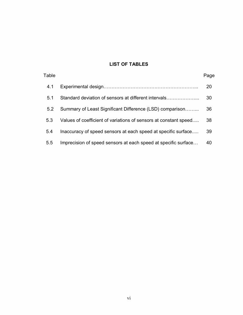
LIST OF TABLES
Table Page
4.1 Experimental design�������������������... 20
5.1 Standard deviation of sensors at different intervals������... 30
5.2 Summary of Least Significant Difference (LSD) comparison��... 36
5.3 Values of coefficient of variations of sensors at constant speed..... 38
5.4 Inaccuracy of speed sensors at each speed at specific surface..... 39
5.5 Imprecision of speed sensors at each speed at specific surface� 40
vii
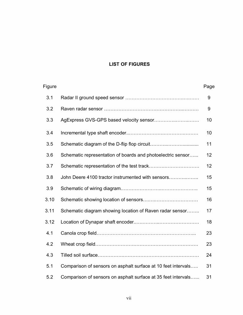
LIST OF FIGURES
Figure Page
3.1 Radar II ground speed sensor ������������.�.�� 9
3.2 Raven radar sensor ����������������..���. 9
3.3 AgExpress GVS-GPS based velocity sensor����..��..��. 10
3.4 Incremental type shaft encoder..�������.����.��� 10
3.5
3.6
3.7
Schematic diagram of the D-flip flop circuit���...���............
Schematic representation of boards and photoelectric sensor�...
Schematic representation of the test track���.�������.
11
12
12
3.8 John Deere 4100 tractor instrumented with sensors���..��.. 15
3.9 Schematic of wiring diagram��������..�������.. 15
3.10 Schematic showing location of sensors�.�.��������� 16
3.11 Schematic diagram showing location of Raven radar sensor��.. 17
3.12 Location of Dynapar shaft encoder..�.���..��������. 18
4.1
4.2
4.3
5.1
5.2
Canola crop field��������������������...
Wheat crop field��������.�������������.
Tilled soil surface�����.����������������
Comparison of sensors on asphalt surface at 10 feet intervals�..
Comparison of sensors on asphalt surface at 35 feet intervals�...
23
23
24
31
31
viii
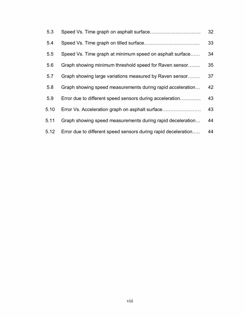
5.3
5.4
5.5
5.6
5.7
5.8
5.9
5.10
5.11
5.12
Speed Vs. Time graph on asphalt surface����������..
Speed Vs. Time graph on tilled surface�����������..
Speed Vs. Time graph at minimum speed on asphalt surface��
Graph showing minimum threshold speed for Raven sensor�..�
Graph showing large variations measured by Raven sensor�..�
Graph showing speed measurements during rapid acceleration�
Error due to different speed sensors during acceleration����.
Error Vs. Acceleration graph on asphalt surface��������
Graph showing speed measurements during rapid deceleration�
Error due to different speed sensors during rapid deceleration.�.
32
33
34
35
37
42
43
43
44
44
1
CHAPTER I
INTRODUCTION
The determination of accurate tractor ground speed is imperative for many
agricultural operations. Ground speed is used as an input for varying the
quantities of fertilizer, pesticides, or herbicides applied. It forms the basis for
optimum application of chemicals thus resulting in minimizing crop inputs and
maximizing profits. In addition, ground speed is also used for controlling the
laying of seeds at optimum distance to improve planting efficiency. Therefore,
determination of accurate and precise tractor speed is critical to optimize the
application of high cost farm inputs. Many speed sensing methods have been
developed to achieve this objective.
In the past, wheel speed sensors were used to measure tractor speed.
These were inaccurate because of low resolution, wheel slip, and loss of surface
and wheel contact. Radar speed measurement systems are commonly used due
to their reasonable cost and acceptable accuracy. However, empirical field
observations indicate that radar ground speed measurements contain increased
error as crop vegetative height increases. A GPS based velocity sensor has been
recently developed that can be used instead of radar sensors and wheel speed
sensors.

2
In this study, two radar sensors and a GPS based velocity sensor were
used for ground speed measurements under varying ground surface conditions.
The responses of these sensors were evaluated compared to a reference speed.
The issues pertaining to measurements of true ground speed were identified and
evaluated with emphasis on addressing the accuracy and precision of these
devices.
1.1 Objectives
The main objectives of this study were to assess:
a) The accuracy and precision of four speed measuring devices under
constant velocity conditions on four different surfaces.
b) The velocity error of three measuring devices during acceleration of the
tractor.
3
CHAPTER II
REVIEW OF LITERATURE
Due to the importance of determining true ground speed for agricultural
applications, numerous studies have been conducted on the subject for more
than three decades. A study by S.S Stuchly et al., (1978) identified the need for
an accurate method of determining the true ground speed of agricultural and
other off-highway equipment. The fifth wheel and free-rolling wheels were
predominantly used to measure ground speed relative to the ground surface
(Luth et al., 1978, Garner et al., 1980, Lin et al., 1980). The ground speed
measurement was also determined by measuring the rotation of tractor front
wheel itself (Grevis-James et al., 1981).
However, the problems associated with measurements of ground speed
using rear or un-driven wheels were identified by Tsuha et al., (1982). The main
problems were:
a) Slippage of rear wheel relative to ground surface.
b) Lifting of un-driven wheels off the ground, thereby resulting in erroneous
measurements in the ground speed.
c) Poor accuracy and resolution.
d) Wheel slip associated with un-driven wheels due to steerage.

4
Therefore, a non-contact ground speed measuring technique was
proposed by using a radar sensor. The absolute accuracy of the radar sensor
was between 1-4% over a variety of surface conditions such as concrete, sand,
mud, asphalt, grass, tiled soil, and moist surfaces. The accuracy of the sensor
was between ± 2% and ± 5% both during controlled field conditions and in actual
working conditions (Tsuha et al., 1982).
N.A. Richardson et al., (1983) identified the limitations on the use of low
cost optical and acoustical sensors. It was concluded that there is very close
correlation between fifth wheel speed measurements and un-driven tractor wheel
measurements, when the tractor is driven on smooth, and firm soil conditions.
The dual beam radar sensor was found to be less sensitive to vehicle motion as
compared to single beam radar sensor.
Tompkins et al., (1985) compared three different type of ground speed
measurement techniques viz., using fifth wheel, front (un-driven wheel), and
radar sensor. The trials were conducted on different surface conditions which
included a smooth, non-deformable surface, various levels of tillage conditions,
and vegetative covers. It was concluded that:
a) There was less slippage of un-driven front wheel compared to fifth wheel.
b) Both front and fifth wheel measurement were in agreement on firm
surfaces.
c) Radar tended to produce accurate results based on a single calibration as
compared to fifth wheel or front (un-driven) wheel.
5
d) The coefficient of variation for ground contacting speed measuring devices
was greater as compared to radar sensors on all test surfaces except for
tall vegetation. It was proposed to calibrate the sensors attached to
ground contacting wheels for specific surface conditions.
G. R. Mueller (1985) did a similar study and concluded that the effect on
accuracy of radar sensors is less due to dense and uniform vegetation as
compared to non-uniform vegetation, for instance corn crops. A dual beam
device was proposed to reduce the variations. Sokol (1985) discussed the use of
a Dickey-John RVS-II radar velocity sensor for agricultural applications and
concluded that the sensor�s accuracy is within ± 2% over variety of terrain
conditions and test course lengths.
Hassan and Sirois (1985) tried a different approach to measure ground
speed by using the stake and stopwatch method. The accuracy and the
resolution improved but had the limitation of preplanned vehicle path. R.D.
Munilla et al., (1988) developed an optical encoder system for wheel rpm and
ground speed. The ground speed encoder had the following drawbacks:
a) The speed measurements were inconclusive.
b) The ground speed encoder accuracy ranged from 10% to 14%.
Stone and Kranzler (1992) developed a prototype of image based ground
velocity sensor. This sensor outperformed both the un-driven wheel-based
measurement and radar system at low speeds but had limitations at higher
speeds. The accuracy of the instrument depended on the optical alignment. The
limitations of this system were:
6
a) Errors or false reading could be generated in case of non-stable ground
reference.
b) Not practically suitable for dusty environment.
c) Increased errors due to unaccountability of pitch and roll changes.
Serrano et al., (2004) investigated the feasibility of low-cost GPS velocity
sensor for vehicle testing application. It was concluded that:
a) The knowledge of satellite position with accuracy level better than 10
meters was necessary to determine vehicle velocity at mm/s level.
b) The error in velocity determination can be due to receiver clock bias that
can be affected by residual atmospheric, multi-path receiver system
noise, and user dynamics as against static mode.
c) The velocity can be estimated better than 1 cm/s in static mode while in
kinematic mode, there was increasing effect of user (receiver) dynamics in
residuals.
7
2.1 Summary
There is an increasing demand for accuracy and precision in many
agricultural applications due to the desire to carefully control the application of
chemicals. Therefore, it is important to investigate the inaccuracies and
imprecision associated with commercially available speed measurement devices.
This study was different from previous works in following aspects:
a) The GPS Velocity sensor was recently developed and was incorporated
for real time speed measurement.
b) All the sensors were calibrated for specific surface conditions as proposed
by Tompkins et al. (1985).
c) Performance of different speed sensors were evaluated for both steady
state and transient conditions.
d) The shaft encoder coupled with un-driven front wheel was considered as a
reference speed as Tompkins et al., (1985) identified that the speed
measurements by using un-driven wheel was in general agreement with
fifth wheel measurement on hard surfaces.
The scope of this work was to assess the precision and accuracy of different
speed measurement techniques as compared to a reference speed sensor under
varying surface conditions.
8
CHAPTER III
HARDWARE OVERVIEW
3.1 Radar sensor
The typical radar speed sensor operates by generating and transmitting
microwaves, which are reflected back with a frequency shift due to movement
between the transmitter / receiver and the target object. This difference in
frequency between the transmitted and the reflected frequency is known as the
Doppler effect (Sokol, 1985). The sensors compare the frequency of reflected
energy with that of emitted energy and this difference is proportional to the
vehicle speed.
The Doppler frequency can be calculated as shown (Sokol,1985):
fd = 2 × VG× cos θ ���������������������.(1) λ
fd = doppler frequency (Hz)
VG= Velocity of the vehicle (miles per second)
λ = Wavelength of transmitted signal (miles)
θ = Angle between ground and sensor (degrees)
The Dickey-John Radar Velocity Sensor-II (DJ RVS-II) works on 24.125
GHz ± 25 MHz microwave frequency with micro power level of 5mw (nominal)
(Sokol, 1985).Two radars of different brands were used for this study as shown in
figures 3.1 and 3.2.

9
Figure 3.1 Radar II ground speed sensor (Source: Dickey-John Corp.)
Figure 3.2 Raven radar sensor (Source: Raven Industries)
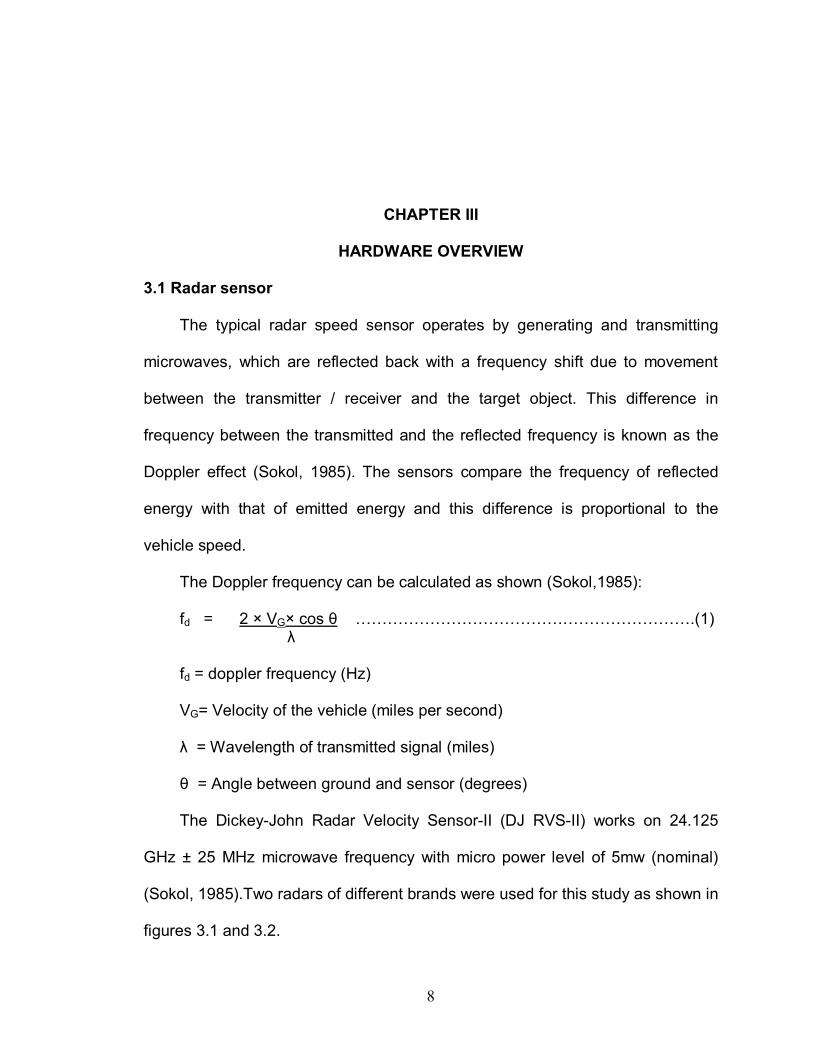
3.2 GPS based velocity sensor
A GPS velocity sensor determines speed by either using the carrier phase
derived Doppler measurement or receiver generated Doppler measurement
(Serrano et al., 2004). A GPS velocity sensor is a cheaper alternative to radar
sensors and is easy to install. An AgExpress GVS-GPS based velocity sensor
was used as shown in figure 3.3 having update frequency of 4 Hz. The sensors
works only when at least 4 or more satellites are in view.
10
Figure 3.3 AgExpress GVS-GPS based velocity sensor (Source: AgExpress Electronics)
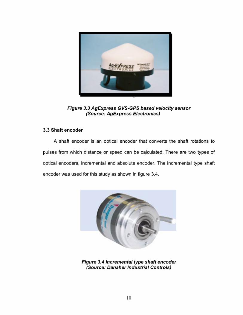
3.3 Shaft encoder
A shaft encoder is an optical encoder that converts the shaft rotations to
pulses from which distance or speed can be calculated. There are two types of
optical encoders, incremental and absolute encoder. The incremental type shaft
encoder was used for this study as shown in figure 3.4.
Figure 3.4 Incremental type shaft encoder
(Source: Danaher Industrial Controls)

11
In addition, the direction of rotation of shaft encoder was determined by
including an electronic circuit comprising of two D-flip flops. The schematic
diagram of the circuit is shown in figure 3.5.
Shaft Encoder
D flip flop
D- flip flop
D
Clk
D
Clk
Q
Q To DAQ unit
To DAQ unit
Black wireRed wire
White Wire
Green wire
5 V D.C
Figure 3.5 Schematic diagram of the D-flip flop circuit (Source: Horowitz and Hill)
This was useful in elimination of ambiguity in the measurements due to
vehicle vibrations to calculate net pulses generated by the encoder during
forward motion of the vehicle.
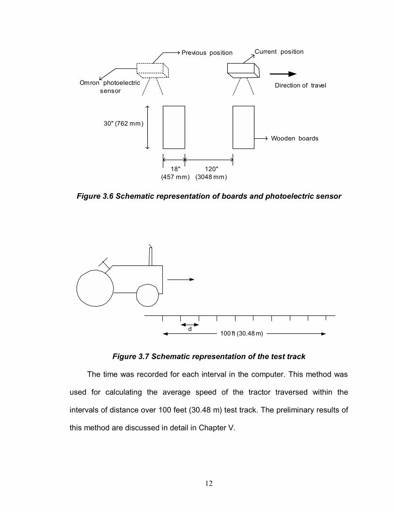
3.4 Photoelectric sensor
A photoelectric sensor was used to time the intervals of distance traversed
by the vehicle over the test track. The wooden boards were painted black in color
to provide contrast for the photoelectric sensor. The boards were placed at
desired intervals of distance over the asphalt surface as shown in figure 3.6.
12
120"(3048 mm)
Direction of travel
Wooden boards
Omron photoelectricsensor
Previous position Current position
18"(457 mm)
30" (762 mm)
Figure 3.6 Schematic representation of boards and photoelectric sensor
Figure 3.7 Schematic representation of the test track
The time was recorded for each interval in the computer. This method was
used for calculating the average speed of the tractor traversed within the
intervals of distance over 100 feet (30.48 m) test track. The preliminary results of
this method are discussed in detail in Chapter V.
100 ft (30.48 m)d
13
3.5 Materials used
The materials used for this project and their technical specifications are
discussed in detail in following sections.
3.5.1 Ground speed sensors
The sensors used for this project were Dickey-John radar (DICKEY-John
Corporation, Auburn, IL), Raven radar (Raven Industries Inc., Sioux Falls, SD),
AgExpress GVS-GPS based velocity sensor (AgExpress Electronics, Grand
Island, NE), Dynapar shaft encoder (Danaher Industrial Controls, Gurnee, IL),
and Omron photoelectric sensor (Omron Electronics Components, Schaumburg,
IL)Omron Electronics LL
3.5.2 Technical details
a) Dickey-John radar velocity sensor (Model Dj RVS-II)
Velocity range: 0.53 to 107 km / hr (0.33 to 67 mph)
Accuracy: <± 5% for speed from 0.53 to 3.2 Km / hr
(0.33 to 2 mph)
<± 3% for speeds from 3.2 to 107 Km / hr
(2 to 67 mph)
Output frequency: 26.11 Hz / Km / hr (44.21 Hz / mph)
Microwave frequency: 24.125 GHz ±50 MHz
b) Raven radar gun / cable
Velocity range: 8.05 to 112.65 km / hr (5 to 70 mph)
Accuracy: Depends on type of console used

14
Output frequency: 58.12 Hz / mph
Microwave frequency: 24.125 GHz
c) AgExpress GVS-GPS based velocity sensor
No. of channels: 16 channel GPS receiver
Accuracy: 0.1mph for speeds from 0.5 to 50 mph
Output frequency: 58.94 Hz / mph
GPS update rate: 4 Hz (4 updates / second)
d) Dynapar Shaft encoder
Resolution: 200 PPR (pulses per revolution)
Accuracy: ± 3 x (360° ÷ PPR) or ± 2.5 arc-min worst case
pulse to any other pulse, whichever is less
e) Photoelectric sensor
Sensing distance: 0 to 70 cm (27.56 inches)
Variation in sensing distance: ± 10% (maximum)
Variation in optical axis and mounting direction: ± 2% (maximum)
Light source: Pulse modulated infrared LED (880nm)
Response time: 1 ms. (maximum)
Standard object: Opaque and transparent materials
Sensitivity: Adjustable
3.5.3 Test vehicle
A John Deere 4100 tractor, owned by the OSU-BAE department, was used
for this project and was instrumented with the sensors and USB based data
acquisition unit as shown in figure 3.8.

15
Figure 3.8 John Deere 4100 tractor instrumented with sensors
3.5.4 Data acquisition and computing equipment
The USB based IOtech DAQ book was installed on the tractor along with a
pentium-based laptop computer to collect sensor information. The IOtech DAQ
book-Personal Daq 56 (IOtech, Inc., Cleveland, Ohio) has 4 frequency / pulse
input channels and 16 digital I/O lines. Figure 3.9 shows the schematic of wiring
diagram.
Figure 3.9 Schematic of wiring diagram
D A Q
1 2 V D .C
D 2
D 1
F 3
F 4
L o
F 1
F 2
S ig n a l fro m D F lip f lo p
S ig n a l fro m P h o to e le c tr ic se n so r
S ig n a l fro m D ick e y -Jo h n s e n s o r
S ig n a l fro m R a ve n se n s o r
S ig n a l fro m A g E x p re ss G V S
S ig n a l F ro m S h a ft e n co d e r
16
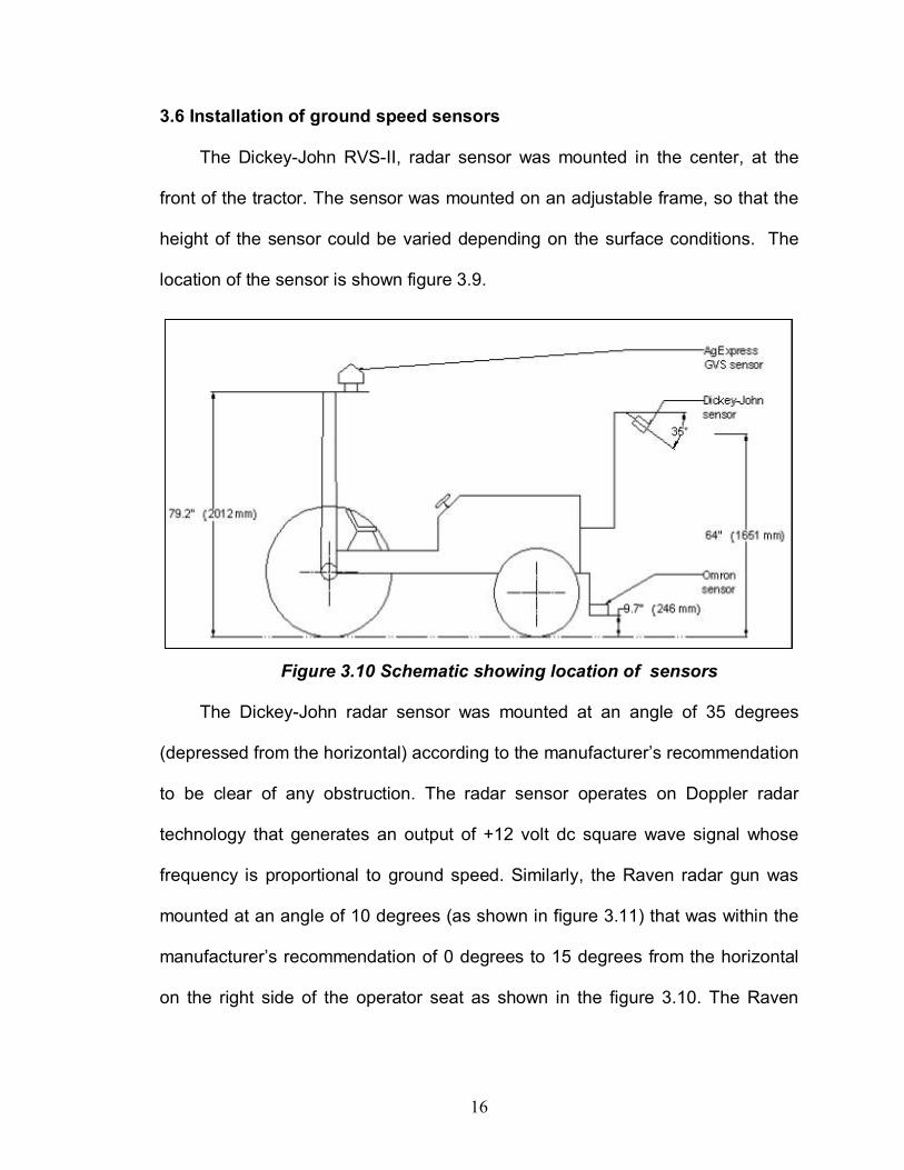
3.6 Installation of ground speed sensors
The Dickey-John RVS-II, radar sensor was mounted in the center, at the
front of the tractor. The sensor was mounted on an adjustable frame, so that the
height of the sensor could be varied depending on the surface conditions. The
location of the sensor is shown figure 3.9.
Figure 3.10 Schematic showing location of sensors
The Dickey-John radar sensor was mounted at an angle of 35 degrees
(depressed from the horizontal) according to the manufacturer�s recommendation
to be clear of any obstruction. The radar sensor operates on Doppler radar
technology that generates an output of +12 volt dc square wave signal whose
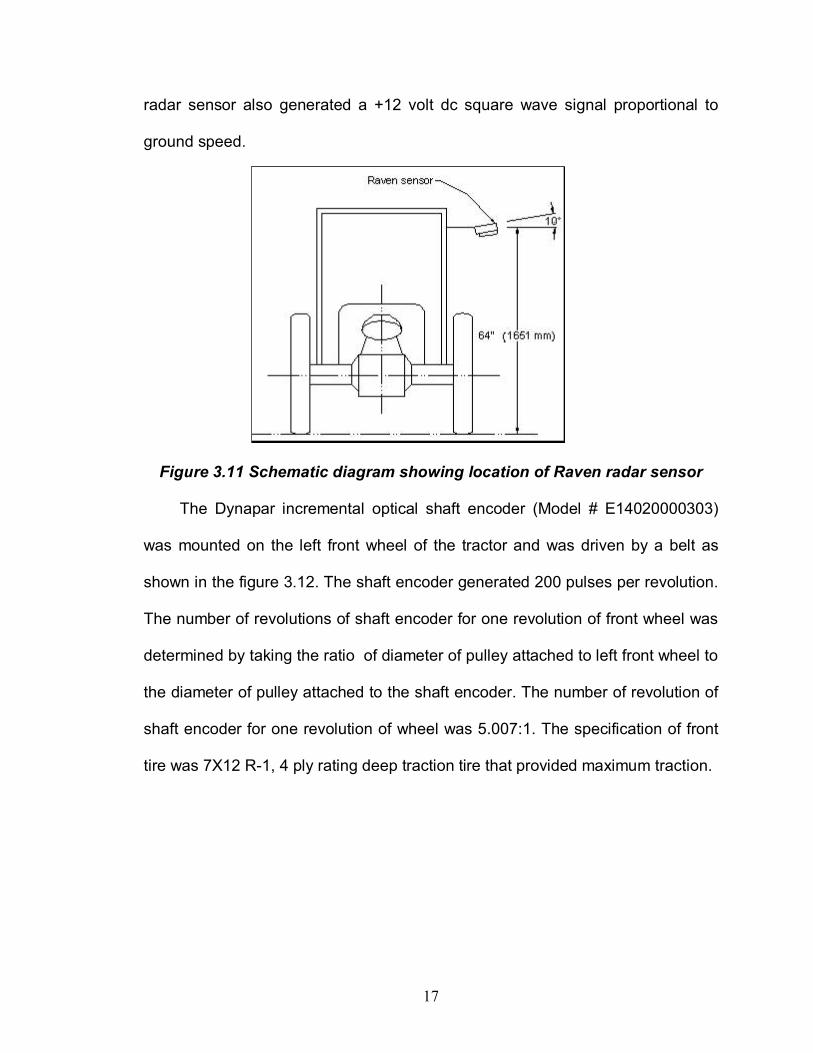
frequency is proportional to ground speed. Similarly, the Raven radar gun was
mounted at an angle of 10 degrees (as shown in figure 3.11) that was within the
manufacturer�s recommendation of 0 degrees to 15 degrees from the horizontal
on the right side of the operator seat as shown in the figure 3.10. The Raven
17
radar sensor also generated a +12 volt dc square wave signal proportional to
ground speed.
Figure 3.11 Schematic diagram showing location of Raven radar sensor
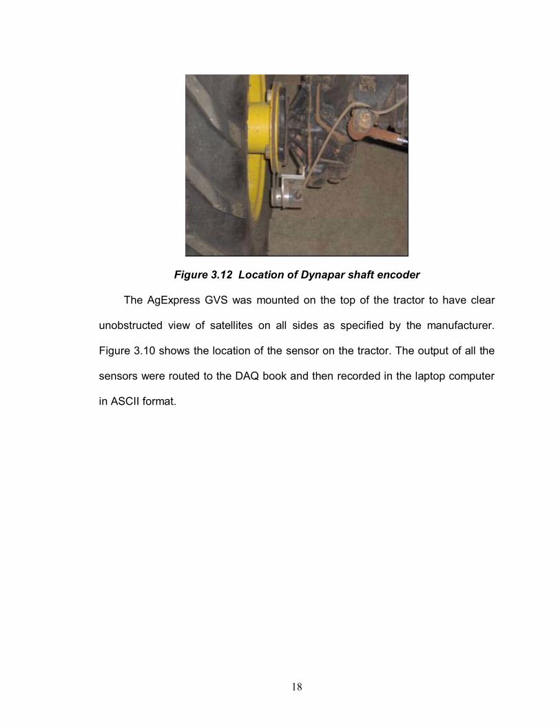
The Dynapar incremental optical shaft encoder (Model # E14020000303)
was mounted on the left front wheel of the tractor and was driven by a belt as
shown in the figure 3.12. The shaft encoder generated 200 pulses per revolution.
The number of revolutions of shaft encoder for one revolution of front wheel was
determined by taking the ratio of diameter of pulley attached to left front wheel to
the diameter of pulley attached to the shaft encoder. The number of revolution of
shaft encoder for one revolution of wheel was 5.007:1. The specification of front
tire was 7X12 R-1, 4 ply rating deep traction tire that provided maximum traction.
18
Figure 3.12 Location of Dynapar shaft encoder
The AgExpress GVS was mounted on the top of the tractor to have clear
unobstructed view of satellites on all sides as specified by the manufacturer.
Figure 3.10 shows the location of the sensor on the tractor. The output of all the
sensors were routed to the DAQ book and then recorded in the laptop computer
in ASCII format.
19
CHAPTER IV
EXPERIMENTAL DESIGN
4.1 Preliminary tests
The initial trial runs were done on an asphalt surface. The optical sensor
was used for sensing the wooden boards placed at specific intervals of 10, 15,
20, 25, 30, and 35 feet (3.05, 4.57, 6.10, 7.62, 9.14, and 10.67 m) respectively
over the test track. The tractor was driven to maintain a speed of 5 mph (8.05
kmph). The time elapsed for the distance traversed through the intervals was
taken from the computer clock and average speed was calculated for each
interval within the 100 feet (30.48 m) track as shown in figure 3.6. The purpose of
these trials were to determine the practical minimum distance interval within the
100 feet (30.48 m) course to calculate the average speed for these intervals and
then compare them with measurements made by other speed sensors. The
results are discussed in Chapter V.
4.2 Test procedure
The four test surface conditions selected were:
a) Asphalt.
b) Vegetative cover with crop height ranging from 0.3-0.5 m.
c) Vegetative cover with crop height ranging from 0.5-1.0 m.
d) Tilled soil conditions where secondary tillage was done.
20
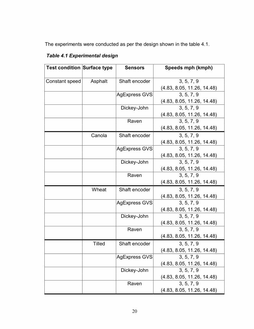
The experiments were conducted as per the design shown in the table 4.1.
Table 4.1 Experimental design
Test condition Surface type Sensors Speeds mph (kmph)
3, 5, 7, 9 Constant speed Asphalt Shaft encoder (4.83, 8.05, 11.26, 14.48)
3, 5, 7, 9 AgExpress GVS(4.83, 8.05, 11.26, 14.48)
3, 5, 7, 9 Dickey-John (4.83, 8.05, 11.26, 14.48)
3, 5, 7, 9 Raven (4.83, 8.05, 11.26, 14.48)
3, 5, 7, 9 Canola Shaft encoder (4.83, 8.05, 11.26, 14.48)
3, 5, 7, 9 AgExpress GVS(4.83, 8.05, 11.26, 14.48)
3, 5, 7, 9 Dickey-John (4.83, 8.05, 11.26, 14.48)
3, 5, 7, 9 Raven (4.83, 8.05, 11.26, 14.48)
3, 5, 7, 9 Wheat Shaft encoder (4.83, 8.05, 11.26, 14.48)
3, 5, 7, 9 AgExpress GVS(4.83, 8.05, 11.26, 14.48)
3, 5, 7, 9 Dickey-John (4.83, 8.05, 11.26, 14.48)
3, 5, 7, 9 Raven (4.83, 8.05, 11.26, 14.48)
3, 5, 7, 9 Tilled Shaft encoder (4.83, 8.05, 11.26, 14.48)
3, 5, 7, 9 AgExpress GVS(4.83, 8.05, 11.26, 14.48)
3, 5, 7, 9 Dickey-John (4.83, 8.05, 11.26, 14.48)
3, 5, 7, 9 Raven (4.83, 8.05, 11.26, 14.48)
21
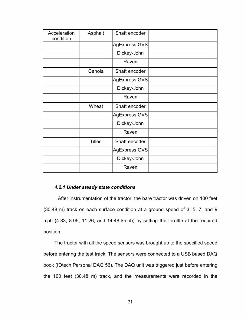
Acceleration condition
Asphalt Shaft encoder
AgExpress GVS
Dickey-John
Raven
Canola Shaft encoder
AgExpress GVS
Dickey-John
Raven
Wheat Shaft encoder
AgExpress GVS
Dickey-John
Raven
Tilled Shaft encoder
AgExpress GVS
Dickey-John
Raven
4.2.1 Under steady state conditions
After instrumentation of the tractor, the bare tractor was driven on 100 feet
(30.48 m) track on each surface condition at a ground speed of 3, 5, 7, and 9
mph (4.83, 8.05, 11.26, and 14.48 kmph) by setting the throttle at the required
position.
The tractor with all the speed sensors was brought up to the specified speed
before entering the test track. The sensors were connected to a USB based DAQ
book (IOtech Personal DAQ 56). The DAQ unit was triggered just before entering
the 100 feet (30.48 m) track, and the measurements were recorded in the

22
computer connected to data acquisition unit until the tractor went past the end
point of the track. The start points, the intermediate points, and the end points
were sensed by a photoelectric sensor on the asphalt track to get the information
of the distance traversed by the tractor at regular intervals during the elapsed
time. The time was recorded both by the computer clock and by a stop watch
(having a least count of 0.01 seconds). The pulses from the sensors were
sampled at an interval of 119 ms. All the sensors were calibrated for specific
surface condition as explained in calibration procedure section in this chapter.
4.2.2 Under transient conditions
a) Vehicle under rapid acceleration
The tractor was driven at approximately 4 mph (6.44 kmph) in high gear
and then rapidly accelerated by increasing the throttle so that the tractor was
driven at maximum achievable speed without drawbar loading on different
surface conditions. The measurements were recorded using the data acquisition
system.
b) Vehicle under rapid deceleration
Similarly, the tractor was decelerated from maximum achievable speed in
high gear to 4 mph (6.44 kmph) (approximately) speed by reducing the throttle
to the desired position. The measurements were recorded using the data
acquisition system and the results are discussed in detail in chapter V.
The trials were replicated six times. This was done to study the transient
behavior of all speed measuring devices during velocity ramp up and ramp down
conditions in addition to assessing the accuracy of all the devices.
23
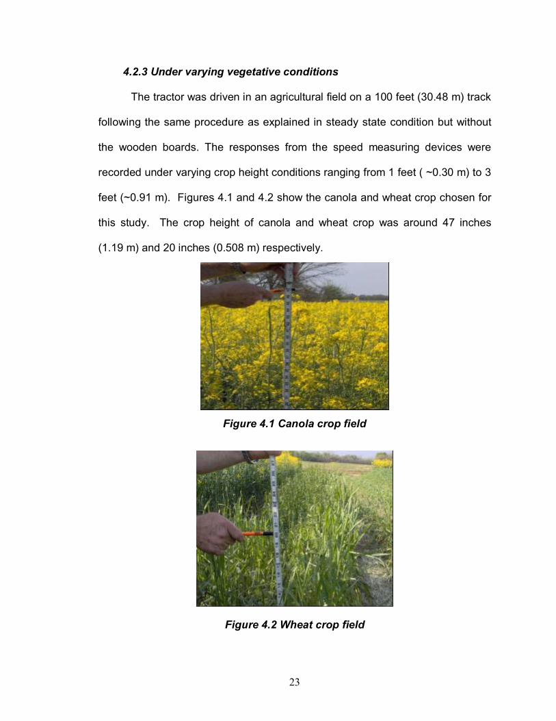
4.2.3 Under varying vegetative conditions
The tractor was driven in an agricultural field on a 100 feet (30.48 m) track
following the same procedure as explained in steady state condition but without
the wooden boards. The responses from the speed measuring devices were
recorded under varying crop height conditions ranging from 1 feet ( ~0.30 m) to 3
feet (~0.91 m). Figures 4.1 and 4.2 show the canola and wheat crop chosen for
this study. The crop height of canola and wheat crop was around 47 inches
(1.19 m) and 20 inches (0.508 m) respectively.
Figure 4.1 Canola crop field
Figure 4.2 Wheat crop field
24
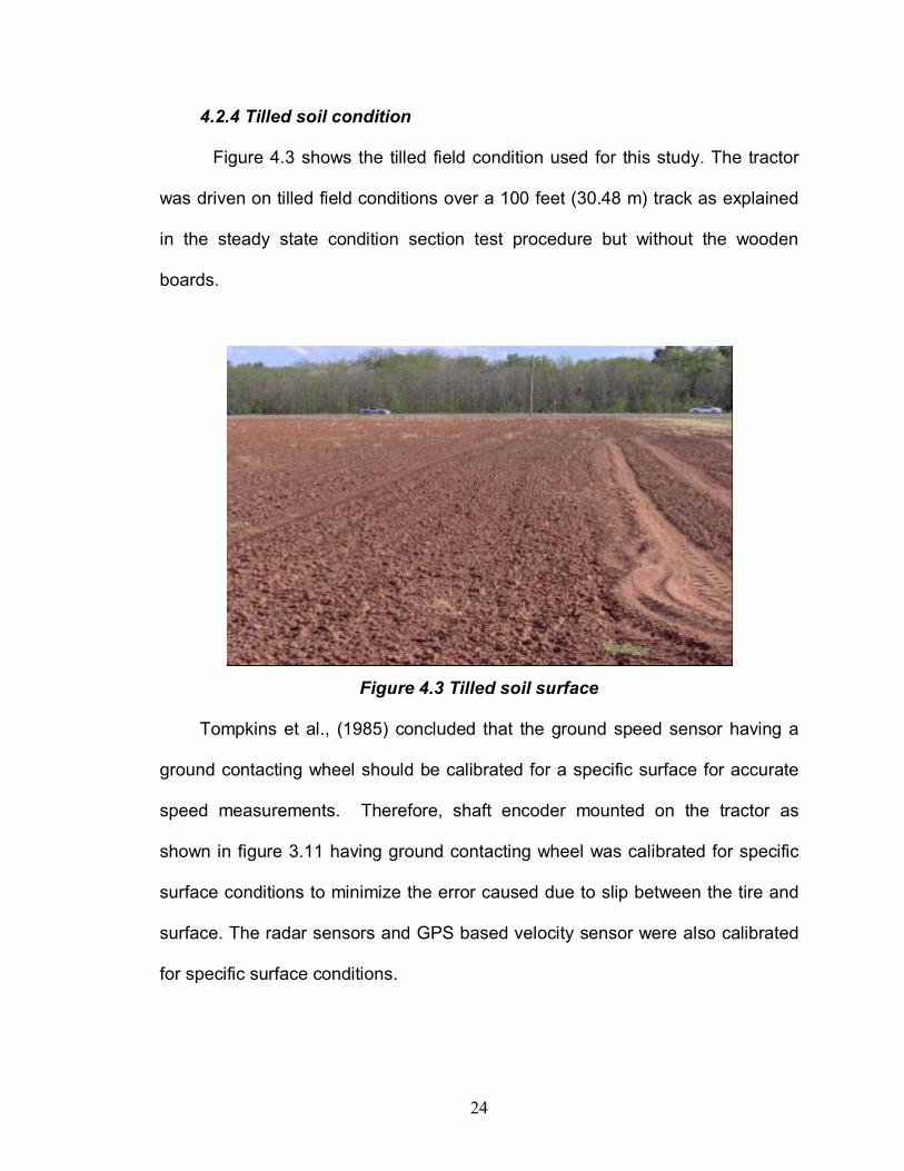
4.2.4 Tilled soil condition
Figure 4.3 shows the tilled field condition used for this study. The tractor
was driven on tilled field conditions over a 100 feet (30.48 m) track as explained
in the steady state condition section test procedure but without the wooden
boards.
Figure 4.3 Tilled soil surface
Tompkins et al., (1985) concluded that the ground speed sensor having a
ground contacting wheel should be calibrated for a specific surface for accurate
speed measurements. Therefore, shaft encoder mounted on the tractor as
shown in figure 3.11 having ground contacting wheel was calibrated for specific
surface conditions to minimize the error caused due to slip between the tire and
surface. The radar sensors and GPS based velocity sensor were also calibrated
for specific surface conditions.

25
4.3 Calibration procedure
The calibration procedure for all the sensors is discussed in detail.
4.3.1 Shaft encoder calibration
The instrumented tractor was driven over a measured distance of 100 feet
(30.48 m) at 3, 5, 7, and 9 mph (4.83, 8.05, 11.26, and 14.48 kmph) speed
respectively without any drawbar load. The total pulses generated by the shaft
encoder were counted for each trial using IOtech DAQ 56 and was recorded in
the computer.
The following formula were used to calibrate the shaft encoder:
P = Total number of pulses for traversing 100 feet (30.48 m)
A = Pulses / revolution of shaft encoder
R se = Total no. of revolutions of shaft encoder
C = Reduction Ratio
D w = Diameter of pulley attached to the wheel hub
D se = Diameter of pulley attached to shaft encoder
t = time elapsed
Total number of revolutions of shaft encoder (n se) = P / A��������...(2)
No. of revolutions of wheel for 100 feet (30.48 m) distance (n w) = R se / C��.(3)
Where,
C = D w / D se������������������ �����..�..(4) Distance traveled for one revolution of wheel (d w ) = 100 feet ���...� �(5)
n w Speed was calculated by
Speed (mph) = P × d w × K ����������������..(6) C × t × A
26
Where,
K = 0.6804 (constant) to express values of speed in miles per hour
K = 1.0950 (constant) to express values of speed in kilometers per hour
This method was followed for all surface conditions.
4.3.2 Radar sensors calibration
The radar sensors were calibrated by driving the tractor over a measured
distance of 100 feet (30.48 m). The calibration value was determined by
comparing the theoretical output with actual output signal for each surface
condition.
The output signal for Dickey-John radar sensor was 30.08 pulses / feet
(99 pulses / meter) and for Raven radar sensor was 39.6 pulses / feet (130
pulses / meter). The actual signal output was measured and compared with
theoretical output signal for determining the calibration value for each surface
condition.
4.3.3 GVS-GPS based velocity sensor calibration
The instrumented vehicle was driven over a measured distance of 100 ft
(30.48 m). The output signal from the GVS was compared with theoretical output
signal for the determination of calibration value. The output signal for GVS
sensor was 40.10 pulses / feet (132 pulses / meter).
27
4.4 Sample size determination
The sample size was determined statistically as explained by Steel et. al,
1997. The number of trials or replications for each treatment depends on:
a) Estimate of σ2
b) Size of the difference to be detected
c) Assurance to detect the desired difference (Power of the test equals 1-β)
d) Level of significance in actual experiment (Type I error)
e) Type of test, whether single or two-tailed
Practically, the estimation of σ2 can be obtained from previous
experiments or by expressing δ as multiple of true standard deviation, σ.
Mathematically, the number of sample size to be replicated for two tailed
test can be calculated by the given formula (Steel et. al, 1997)
r ≥ 2 × (t α/2 + tβ) 2 × (σ/ δ)2 ������������......(7)
Where,
r = number of observations on each treatment
σ = estimate of standard deviation
δ = differences in mean
The subscripts of �t� are based on Type I and Type II error and the values can be
referred to the probability in a single tail of the t distribution.
In this study, the desired significance level α was 1% and β was 10% with
90 percent assurance of detecting the differences. Thus, the value of t α/2 = 2.015
and the value of tβ = 1.28. The value of �σ� as estimated conservatively from initial
trial runs was 0.1 and the desired value of δ = 0.1 mph. Replacing the values of t
28
α/2, tβ, σ, and δ in the equation (7), we get the number of observations for each
treatment �r� equal to 6. Based on this calculation, all the trials were replicated six
times under different surface conditions to evaluate the precision of the speed
measuring devices. The results of precision errors and the accuracy of these
devices are discussed in chapter V.
29
CHAPTER V
RESULTS AND DISCUSSIONS
5.1 Determination of a �reference� speed sensor
It was important to determine a true reference speed for comparing
measurements by different speed measuring devices. The initial trials were
conducted on an asphalt surface with a photoelectric sensor mounted on the
tractor. The following steps explain the method for measurement of true ground
speed using the photoelectric sensor.
a) The 100 feet (30.48 m) track was subdivided into different intervals of 10,
15, 20, 25, 30, and 35 feet (3.05, 4.57, 6.10, 7.62, 9.14, and 10.67 m).
b) The tractor mounted with the speed sensors was driven at a speed of 5
mph on asphalt surface.
c) The time elapsed for traversing each intervals within 100 feet (30.48 m)
(as shown in figure 3.6) was recorded using a laptop computer.
d) The average speed was calculated for each interval.
e) This method was used to calculate the average speed over the specified
intervals and then compare the average speed measured by other devices
for the same stretch. The advantage of using photoelectric sensor was
that it had no effect of factors like wind or wheel slip.
30
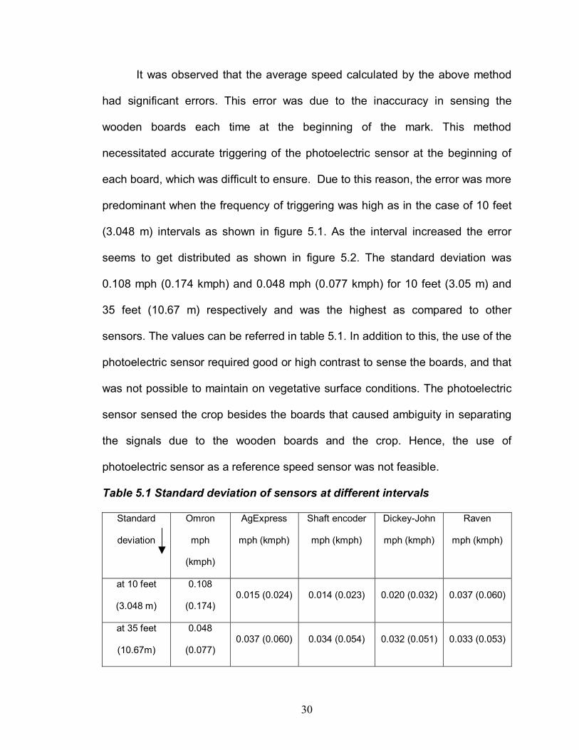
It was observed that the average speed calculated by the above method
had significant errors. This error was due to the inaccuracy in sensing the
wooden boards each time at the beginning of the mark. This method
necessitated accurate triggering of the photoelectric sensor at the beginning of
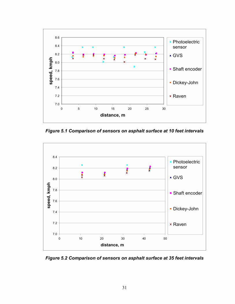
each board, which was difficult to ensure. Due to this reason, the error was more
predominant when the frequency of triggering was high as in the case of 10 feet
(3.048 m) intervals as shown in figure 5.1. As the interval increased the error
seems to get distributed as shown in figure 5.2. The standard deviation was
0.108 mph (0.174 kmph) and 0.048 mph (0.077 kmph) for 10 feet (3.05 m) and
35 feet (10.67 m) respectively and was the highest as compared to other
sensors. The values can be referred in table 5.1. In addition to this, the use of the
photoelectric sensor required good or high contrast to sense the boards, and that
was not possible to maintain on vegetative surface conditions. The photoelectric
sensor sensed the crop besides the boards that caused ambiguity in separating
the signals due to the wooden boards and the crop. Hence, the use of
photoelectric sensor as a reference speed sensor was not feasible.
Table 5.1 Standard deviation of sensors at different intervals
Standard
deviation
Omron
mph
(kmph)
AgExpress
mph (kmph)
Shaft encoder
mph (kmph)
Dickey-John
mph (kmph)
Raven
mph (kmph)
at 10 feet
(3.048 m)
0.108
(0.174) 0.015 (0.024) 0.014 (0.023) 0.020 (0.032) 0.037 (0.060)
at 35 feet
(10.67m)
0.048
(0.077) 0.037 (0.060) 0.034 (0.054) 0.032 (0.051) 0.033 (0.053)
31
Figure 5.1 Comparison of sensors on asphalt surface at 10 feet intervals
Figure 5.2 Comparison of sensors on asphalt surface at 35 feet intervals
7.0
7.2
7.4
7.6
7.8
8.0
8.2
8.4
8.6
0 5 10 15 20 25 30
distance, m
spee
d, k
mph
Photoelectricsensor
GVS
Shaft encoder
Dickey-John
Raven
7.0
7.2
7.4
7.6
7.8
8.0
8.2
8.4
0 10 20 30 40 50
distance, m
spee
d, k
mph
Photoelectricsensor
GVS
Shaft encoder
Dickey-John
Raven
32
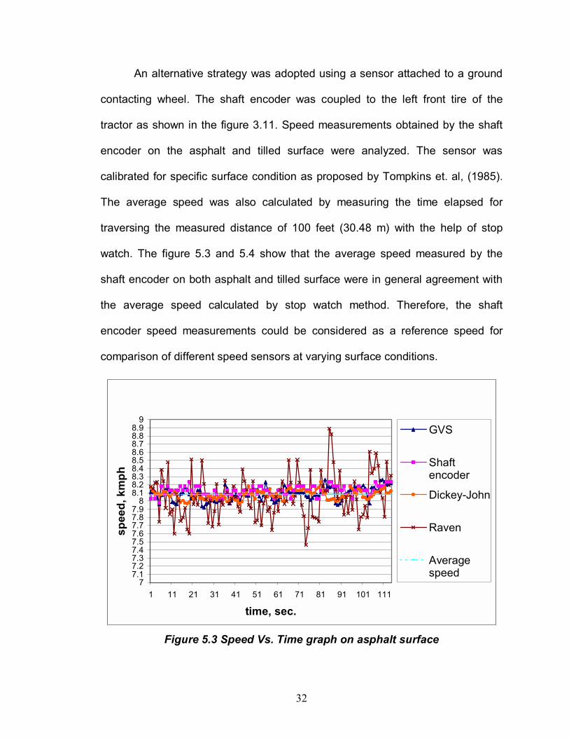
An alternative strategy was adopted using a sensor attached to a ground
contacting wheel. The shaft encoder was coupled to the left front tire of the
tractor as shown in the figure 3.11. Speed measurements obtained by the shaft
encoder on the asphalt and tilled surface were analyzed. The sensor was
calibrated for specific surface condition as proposed by Tompkins et. al, (1985).
The average speed was also calculated by measuring the time elapsed for
traversing the measured distance of 100 feet (30.48 m) with the help of stop
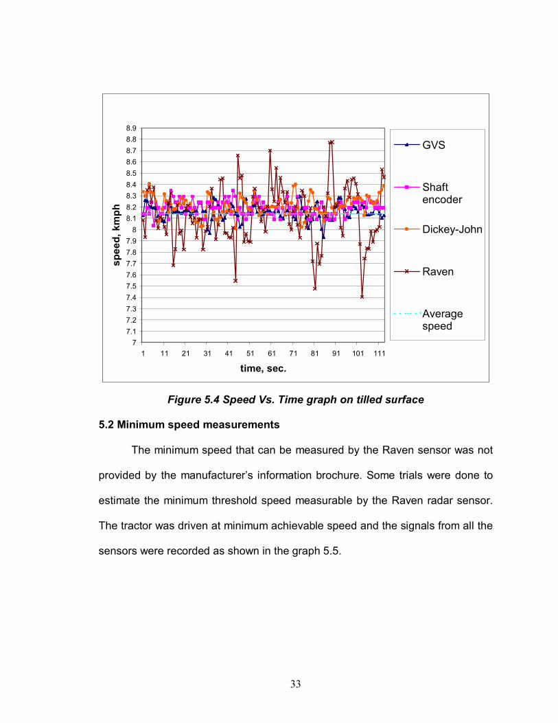
watch. The figure 5.3 and 5.4 show that the average speed measured by the
shaft encoder on both asphalt and tilled surface were in general agreement with
the average speed calculated by stop watch method. Therefore, the shaft
encoder speed measurements could be considered as a reference speed for
comparison of different speed sensors at varying surface conditions.
Figure 5.3 Speed Vs. Time graph on asphalt surface
77.17.27.37.47.57.67.77.87.9
88.18.28.38.48.58.68.78.88.9
9
1 11 21 31 41 51 61 71 81 91 101 111
time, sec.
spee
d, k
mph
GVS
Shaftencoder
Dickey-John
Raven
Averagespeed
33
Figure 5.4 Speed Vs. Time graph on tilled surface
5.2 Minimum speed measurements
The minimum speed that can be measured by the Raven sensor was not
provided by the manufacturer�s information brochure. Some trials were done to
estimate the minimum threshold speed measurable by the Raven radar sensor.
The tractor was driven at minimum achievable speed and the signals from all the
sensors were recorded as shown in the graph 5.5.
77.17.27.37.47.57.67.77.87.9
88.18.28.38.48.58.68.78.88.9
1 11 21 31 41 51 61 71 81 91 101 111
time, sec.
spee
d, k
mph
GVS
Shaftencoder
Dickey-John
Raven
Averagespeed

34
Figure 5.5 Speed Vs. Time graph at minimum speed on asphalt surface
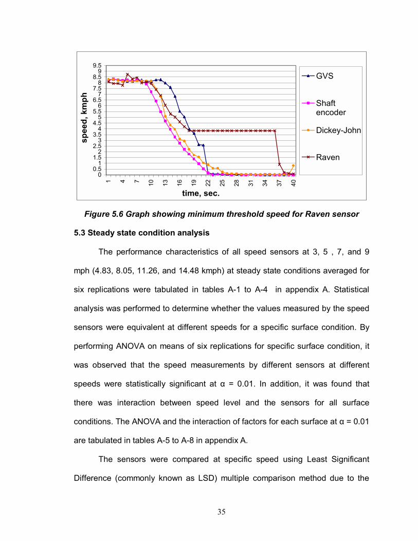
This graph shows that speed measured by the Raven radar sensor varied
from 0 mph (0 kmph) to little over 3 mph (4.83 kmph) when the actual forward
speed of the vehicle was close to 1.6 mph (2.57 kmph). This was probably due to
the inherent design characteristics of the device. On further investigation during
transient conditions, it was observed that there was a minimum threshold speed
of 2.5 mph (4.02 kmph) and the sensor did not work well below this speed. This
is shown in the figure 5.6.
0
0.5
1
1.5
2
2.5
3
3.5
4
4.5
5
5.5
1 21 41 61 81 101
121
141
161
181
201
221
241
261
281
301
321
time, sec.
spee
d, k
mph
GVS
Shaftencoder
Dickey-John
Raven
35
Figure 5.6 Graph showing minimum threshold speed for Raven sensor
5.3 Steady state condition analysis
The performance characteristics of all speed sensors at 3, 5 , 7, and 9
mph (4.83, 8.05, 11.26, and 14.48 kmph) at steady state conditions averaged for
six replications were tabulated in tables A-1 to A-4 in appendix A. Statistical
analysis was performed to determine whether the values measured by the speed
sensors were equivalent at different speeds for a specific surface condition. By
performing ANOVA on means of six replications for specific surface condition, it
was observed that the speed measurements by different sensors at different
speeds were statistically significant at α = 0.01. In addition, it was found that
there was interaction between speed level and the sensors for all surface
conditions. The ANOVA and the interaction of factors for each surface at α = 0.01
are tabulated in tables A-5 to A-8 in appendix A.
The sensors were compared at specific speed using Least Significant
Difference (commonly known as LSD) multiple comparison method due to the
00.5
11.5
22.5
33.5
44.5
55.5
66.5
77.5
88.5
99.5
1 4 7 10 13 16 19 22 25 28 31 34 37 40
time, sec.
spee
d, k
mph
GVS
Shaftencoder
Dickey-John
Raven
36
interaction between speed level and sensors. The results of the comparison of
different speed sensors at each speed for specific surface conditions relative to
shaft encoder are summarized in table 5.2.
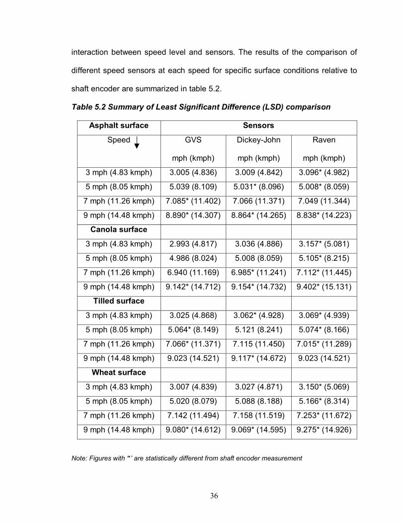
Table 5.2 Summary of Least Significant Difference (LSD) comparison
Asphalt surface Sensors
Speed GVS
mph (kmph)
Dickey-John
mph (kmph)
Raven
mph (kmph)
3 mph (4.83 kmph) 3.005 (4.836) 3.009 (4.842) 3.096* (4.982)
5 mph (8.05 kmph) 5.039 (8.109) 5.031* (8.096) 5.008* (8.059)
7 mph (11.26 kmph) 7.085* (11.402) 7.066 (11.371) 7.049 (11.344)
9 mph (14.48 kmph) 8.890* (14.307) 8.864* (14.265) 8.838* (14.223)
Canola surface
3 mph (4.83 kmph) 2.993 (4.817) 3.036 (4.886) 3.157* (5.081)
5 mph (8.05 kmph) 4.986 (8.024) 5.008 (8.059) 5.105* (8.215)
7 mph (11.26 kmph) 6.940 (11.169) 6.985* (11.241) 7.112* (11.445)
9 mph (14.48 kmph) 9.142* (14.712) 9.154* (14.732) 9.402* (15.131)
Tilled surface
3 mph (4.83 kmph) 3.025 (4.868) 3.062* (4.928) 3.069* (4.939)
5 mph (8.05 kmph) 5.064* (8.149) 5.121 (8.241) 5.074* (8.166)
7 mph (11.26 kmph) 7.066* (11.371) 7.115 (11.450) 7.015* (11.289)
9 mph (14.48 kmph) 9.023 (14.521) 9.117* (14.672) 9.023 (14.521)
Wheat surface
3 mph (4.83 kmph) 3.007 (4.839) 3.027 (4.871) 3.150* (5.069)
5 mph (8.05 kmph) 5.020 (8.079) 5.088 (8.188) 5.166* (8.314)
7 mph (11.26 kmph) 7.142 (11.494) 7.158 (11.519) 7.253* (11.672)
9 mph (14.48 kmph) 9.080* (14.612) 9.069* (14.595) 9.275* (14.926)
Note: Figures with �*� are statistically different from shaft encoder measurement
37
In general, AgExpress GVS and Dickey-John sensor were in agreement
with shaft encoder measurements under vegetative conditions except at higher
speeds. Raven radar was significantly different in most of the cases from the
shaft encoder speed measurements due to higher variability in the speed
measurements. The Raven radar measurements for 3 mph (4.83 kmph) were
documented though it was later communicated by Raven�s representative that
the minimum speed that can be measured by the sensor is 5 mph (8.05 kmph).
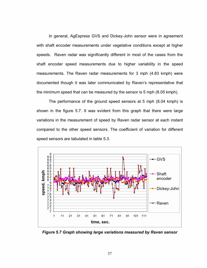
The performance of the ground speed sensors at 5 mph (8.04 kmph) is
shown in the figure 5.7. It was evident from this graph that there were large
variations in the measurement of speed by Raven radar sensor at each instant
compared to the other speed sensors. The coefficient of variation for different
speed sensors are tabulated in table 5.3.
Figure 5.7 Graph showing large variations measured by Raven sensor
77.17.27.37.47.57.67.77.87.9
88.18.28.38.48.58.68.78.88.9
9
1 11 21 31 41 51 61 71 81 91 101 111
time, sec.
spee
d, k
mph
GVS
Shaftencoder
Dickey-John
Raven

38
Table 5.3 Values of coefficient of variations of sensors at constant speed
Sensor type Coefficient of variation
AgExpress GVS 0.25 % - 2.2 %
Dickey-John 0.2 % - 1.7 %
Raven 0.61 % - 1.78 %
Similarly, the results of ANOVA at α = 0.01 revealed that the standard
deviation of AgExpress GVS and Dickey-John speed sensor were in general
agreement with the shaft encoder except at 9 mph (14.48 kmph) speed. The
standard deviation of Raven radar data was significantly different from that of the
shaft encoder as well.
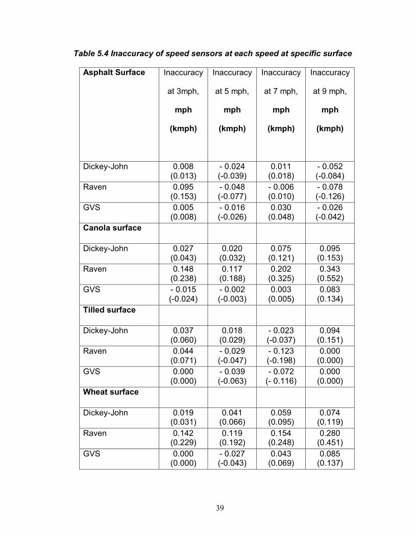
The inaccuracy of the speed sensors were calculated by taking difference
between the mean of speed measurement of six replications and the test unit at
each speed for specific surface conditions. The values are tabulated in table 5.4.
Similarly, the imprecision values were the twice the standard deviation of six
replications at each speed for specific surface conditions as mentioned in the
NIST Guideline (1994) and are tabulated in table 5.5. The tables A-1 to A-4 in
appendix A can be referred for the speed and the standard deviation values of
each device at each speed for specific surface condition.
39
Table 5.4 Inaccuracy of speed sensors at each speed at specific surface
Asphalt Surface Inaccuracy
at 3mph,
mph
(kmph)
Inaccuracy
at 5 mph,
mph
(kmph)
Inaccuracy
at 7 mph,
mph
(kmph)
Inaccuracy
at 9 mph,
mph
(kmph)
Dickey-John 0.008 (0.013)
- 0.024 (-0.039)
0.011 (0.018)
- 0.052 (-0.084)
Raven 0.095 (0.153)
- 0.048 (-0.077)
- 0.006 (0.010)
- 0.078 (-0.126)
GVS 0.005 (0.008)
- 0.016 (-0.026)
0.030 (0.048)
- 0.026 (-0.042)
Canola surface
Dickey-John 0.027 (0.043)
0.020 (0.032)
0.075 (0.121)
0.095 (0.153)
Raven 0.148 (0.238)
0.117 (0.188)
0.202 (0.325)
0.343 (0.552)
GVS - 0.015 (-0.024)
- 0.002 (-0.003)
0.003 (0.005)
0.083 (0.134)
Tilled surface
Dickey-John 0.037 (0.060)
0.018 (0.029)
- 0.023 (-0.037)
0.094 (0.151)
Raven 0.044 (0.071)
- 0.029 (-0.047)
- 0.123 (-0.198)
0.000 (0.000)
GVS 0.000 (0.000)
- 0.039 (-0.063)
- 0.072 (- 0.116)
0.000 (0.000)
Wheat surface
Dickey-John 0.019 (0.031)
0.041 (0.066)
0.059 (0.095)
0.074 (0.119)
Raven 0.142 (0.229)
0.119 (0.192)
0.154 (0.248)
0.280 (0.451)
GVS 0.000 (0.000)
- 0.027 (-0.043)
0.043 (0.069)
0.085 (0.137)

40
Table 5.5 Imprecision of speed sensors at each speed at specific surface
Asphalt Surface Imprecision
at 3mph,
mph (kmph)
Imprecision
at 5 mph,
mph (kmph)
Imprecision
at 7 mph,
mph (kmph)
Imprecision
at 9 mph,
mph (kmph)
Dickey-John ± 0.014 (± 0.023)
± 0.028 (± 0.045)
± 0.038 (± 0.061)
± 0.018 (± 0.029)
Raven ± 0.022 (± 0.035)
± 0.038 (± 0.061)
± 0.054 (± 0.087)
± 0.054 (± 0.087)
GVS ± 0.012 (± 0.019)
± 0.024 (± 0.039)
± 0.030 (± 0.048)
± 0.022 (± 0.035)
Canola surface
Dickey-John ± 0.018 (± 0.029)
± 0.086 (± 0.138)
± 0.040 (± 0.064)
± 0.054 (± 0.087)
Raven ± 0.036 (± 0.058)
± 0.086 (± 0.138)
± 0.052 (± 0.084)
± 0.104 (± 0.167)
GVS ± 0.066 (± 0.106)
± 0.060 (± 0.097)
± 0.056 (± 0.090)
± 0.154 (± 0.248)
Tilled surface
Dickey-John ± 0.014 (± 0.023)
± 0.030 (± 0.048)
± 0.024 (± 0.039)
± 0.048 (± 0.077)
Raven ± 0.024 (± 0.039)
± 0.054 (± 0.087)
± 0.028 (± 0.045)
± 0.048 (± 0.077)
GVS ± 0.014 (± 0.023)
± 0.026 (± 0.042)
± 0.016 (± 0.026)
± 0.060 (± 0.097)
Wheat surface
Dickey-John ± 0.020 (± 0.032)
± 0.058 (± 0.093)
± 0.044 (± 0.071)
± 0.058 (± 0.093)
Raven ± 0.016 (± 0.026)
± 0.092 (± 0.148)
± 0.082 (± 0.132)
± 0.096 (± 0.154)
GVS ± 0.022 (± 0.035)
± 0.048 (± 0.077)
± 0.184 (± 0.296)
± 0.160 (± 0.257)
41
The AgExpress GVS sensor closely agreed with the shaft encoder in
steady state conditions and could be an inexpensive alternative to radar sensors.
The error in the speed measurements by the Raven radar sensor increased with
increasing speed over canola and wheat surface conditions which might be due
to the canopy effect of the crop. The Dickey-John radar sensor was relatively
accurate on all surface conditions with accuracy level of 0.095 mph (0.153 kmph)
whereas accuracy of the Raven radar sensor was within 0.343 mph (0.552
kmph).
The speed measurements by AgExpress GVS sensor were more precise
except at 9 mph (14.48 kmph) which might be due to the uneven vehicle motion
under vegetative conditions. The Raven sensor on the other hand was least
precise under vegetative conditions as compared to the Dickey-John radar
sensor. This could be due to the waving of crop canopy cover caused by high
wind speeds of 41.0 mph (65.98 kmph). The values of wind speed were taken
from Oklahoma Mesonet website. It was observed that the Dickey-John radar
sensor was consistent in terms of precision across all surfaces.
5.4 Transient state condition analysis
The acceleration and deceleration trials were conducted to analyze the
transient behavior of speed sensors. The Raven radar sensor had limitation of
measuring ground speed below 3 mph (4.83 kmph) as discussed earlier.
Therefore, all the acceleration trials were carried out from 4 mph (6.44 kmph) to
maximum achievable speed, and the deceleration trials were carried out from

42
maximum achievable speed by the vehicle to 4 mph (6.44 kmph)
(approximately).
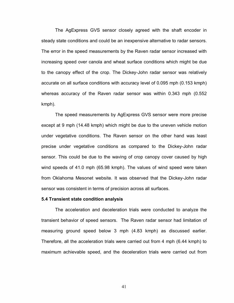
The data were recorded on time domain as shown in the figure 5.8. The
speed measured by the shaft encoder was accurate enough to compare the
behavior of other speed sensors with respect to shaft encoder speed
measurements as discussed before. Table Curve 2D (Aspire Software
International, Leeburg, VA) software was used to process the raw data by fitting
a curve through the shaft encoder speed measurements. The sigmoid function
was selected as the curve model to fit the shaft encoder data thereby eliminating
noise in the shaft encoder measurements.
Figure 5.8 Graph showing speed measurements during rapid acceleration
0
2
4
6
8
10
12
14
16
18
20
22
1 4 7 10 13 16 19 22 25 28 31 34 37 40 43 46 49
time, sec.
spee
d, k
mph
GVS
Shaft encoder
Dickey-John
Raven
43
Figure 5.9 Error due to different speed sensors during acceleration
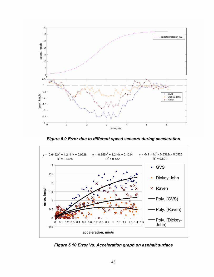
Figure 5.10 Error Vs. Acceleration graph on asphalt surface
0 1 2 3 4 5 6 7-3
-2.5
-2
-1.5
-1
-0.5
0
0.5
time, sec.
erro
r, km
ph
06
8
10
12
14
16
18
20
spee
d, k
mph
Predicted velocity (SE)
GVSDickey-JohnRaven
y = -0.1141x2 + 0.8322x - 0.0525R2 = 0.8911
y = -0.355x2 + 1.244x + 0.1214R2 = 0.482
y = -0.6492x2 + 1.2141x + 0.0628R2 = 0.4728
-0.5
0
0.5
1
1.5
2
2.5
3
0 0.1 0.2 0.3 0.4 0.5 0.6 0.7 0.8 0.9 1 1.1 1.2 1.3 1.4 1.5
acceleration, m/s/s
erro
r, km
ph
GVS
Dickey-John
Raven
Poly. (GVS)
Poly. (Raven)
Poly. (Dickey-John)
44
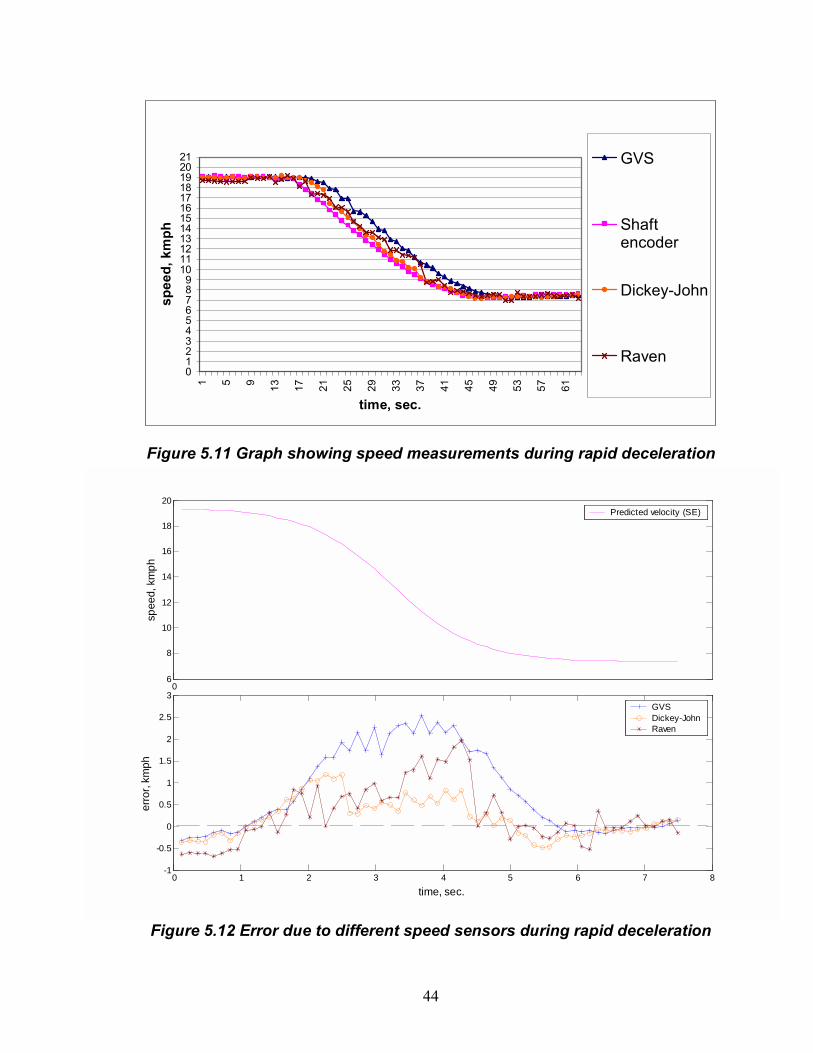
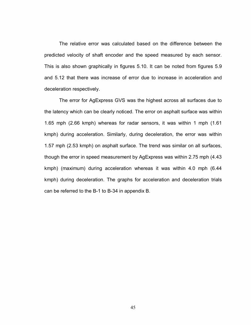
Figure 5.11 Graph showing speed measurements during rapid deceleration
Figure 5.12 Error due to different speed sensors during rapid deceleration
0123456789
101112131415161718192021
1 5 9 13 17 21 25 29 33 37 41 45 49 53 57 61
time, sec.
spee
d, k
mph
GVS
Shaftencoder
Dickey-John
Raven
0 1 2 3 4 5 6 7 8-1
-0.5
0
0.5
1
1.5
2
2.5
3
time, sec.
erro
r, km
ph
06
8
10
12
14
16
18
20
spee
d, k
mp
h
Predicted velocity (SE)
GVSDickey-JohnRaven
45
The relative error was calculated based on the difference between the
predicted velocity of shaft encoder and the speed measured by each sensor.
This is also shown graphically in figures 5.10. It can be noted from figures 5.9
and 5.12 that there was increase of error due to increase in acceleration and
deceleration respectively.
The error for AgExpress GVS was the highest across all surfaces due to
the latency which can be clearly noticed. The error on asphalt surface was within
1.65 mph (2.66 kmph) whereas for radar sensors, it was within 1 mph (1.61
kmph) during acceleration. Similarly, during deceleration, the error was within
1.57 mph (2.53 kmph) on asphalt surface. The trend was similar on all surfaces,
though the error in speed measurement by AgExpress was within 2.75 mph (4.43
kmph) (maximum) during acceleration whereas it was within 4.0 mph (6.44
kmph) during deceleration. The graphs for acceleration and deceleration trials
can be referred to the B-1 to B-34 in appendix B.

46
CHAPTER VI
CONCLUSIONS AND SUMMARY
6.1 Conclusions
The following conclusions can be drawn based on this study:
a) The Dickey-John radar was more precise and consistent as compared to
other speed sensors across all surface conditions. The maximum
imprecision of speed sensors across all surfaces and speeds are
summarized below:
Dickey-John radar sensor ! ± 0.044 mph (± 0.071 kmph)
Raven radar sensor ! ± 0.096 mph (± 0.154 kmph)
AgExpress GVS sensor ! ± 0.184 mph (± 0.296 kmph)
The accuracy of Dickey-John and AgExpress GVS sensors were in
close agreement but significantly different from Raven sensor. The Raven
sensor was more sensitive to vegetative conditions across all speeds. The
maximum inaccuracy of the speed sensors across all surfaces and speeds
were:
Dickey-John radar sensor ! 0.09 mph ( 0.151 kmph)
Raven radar sensor ! 0.34 mph ( 0.552 kmph)
AgExpress GVS sensor ! 0.08 mph ( 0.134 kmph)
47
b) The maximum error in speed measurement during transient conditions for
radar sensors were within 1.0 mph (1.61 kmph) whereas the GPS based
sensor has maximum error within 4.0 mph (6.44 kmph) during acceleration
because of the latency.
6.2 Summary
a) In general, AgExpress GVS and Dickey-John radar sensor were in general
agreement with shaft encoder measurements under vegetative conditions
except at higher speeds.
b) The Raven radar sensor was statistically different from the shaft encoder
The error increased with increase in vehicle speed over wheat and canola
surface. This was due to the effect of wind and waving of crop canopy.
The Dickey-John was less sensitive to crop canopy effect when compared
with Raven radar. It was observed that the Raven radar was least
accurate.
c) The Raven radar can be used for measuring speeds on an average from 3
mph (4.83 kmph) onwards though large variations were observed in speed
measurements.
d) On the other hand, the AgExpress GVS sensor was consistent except at
higher speeds on vegetative surfaces. This might be due to the uneven
vehicle motion and user dynamics. The AgExpress GVS sensor showed
promising results and could be used for speed measurements for steady
state conditions because of its cost advantage.
48
e) During transient conditions, both the radar sensors followed the same
trend. The maximum error in speed measurements by the radar sensors
was close to 1 mph (1.61 kmph) during acceleration and deceleration
conditions across all surfaces whereas the error in speed measurements
by the AgExpress GVS was 2.75 mph (4.43 kmph) (maximum) on the
lower side during acceleration and close to 4 mph (6.44 kmph) during
deceleration. Therefore, it was not suitable for transient condition
applications due to the latency.
6.3 Suggestions for future research
The GPS based speed measuring device shows promising results for use
in agricultural applications under steady state conditions. However, additional
research needs to be done for improving the GPS system under transient
conditions for precision agriculture applications.
The Raven radar sensor had large variations in speed measurements
across all surface. Therefore, it is recommended to reinvestigate the inherent
design of the sensor and improve it for making it insensitive to errors due to
canopy effect or due to pitch, yaw or roll motion of the vehicle. The reference
speed could be measured using an advanced technique such as a laser sensor
for accurate triggering and then recording the time elapsed for specific intervals
using computer.
Further information can by unraveled by conducting the experiment under
different wind speed conditions over the vegetative surface. It is also suggested

49
to chose the vegetative crop based on distribution of the crop density for future
study which might produce useful information on parameters that affect the
speed measurements by radar sensors.
50
REFERENCES
Garner, T.H., D. Wolf, and J.W. Davis. 1980. Tillage energy instrumentation
and field results. Proceedings Beltwide Cotton Production Research
Conferences. National Cotton Council of America, Memphis, TN 38182. pp.
117-120.
Grevis-James, I.W., D.R. Devoe, P.D. Bloome, and D. G. Batchelder. 1981.
Microcomputer based data acquisition system for tractors. ASAE Paper No.
81-1578. American Society of Agricultural Engineers, ST. Joseph MI 49085.
Lin, Tzu-Wei, R.L. Clark, and A.H. Adsit. 1980. A microprocessor based data
acquisition system to measure performance of a small four-wheel drive
tractor. ASAE Paper No. 80-5225. American Society of Agricultural
Engineers, St. Joseph MI 49085.
Luth, H.J., V.G. Floyd, and R.P. Heise.1978. Evaluating energy requirements
of machines in the field. ASAE Paper No. 78-1588. American Society of
Agricultural Engineers, St. Joseph MI 49085.
Munilla, R.D., and Hassan, A.E., Yu, G.S. 1988. An optical encoder for
ground speed measurement. ASAE Paper No. 88-7522. American Society of
Agricultural Engineers, St. Joseph MI 49085.
51
Richardson, N.A., Lanning, R. L., Kopp, K.A., and Carnegie, E.J. 1983. True
Ground Speed Measurement. ASAE (Microfiche collection) Paper No. 83-
1059.
Serrano, L., Kim, D., Langley, R.B., Itani, K., and Ueno, M. 2004. A GPS
Velocity Sensor : How accurate can it be ? � A first look. ION NTM 2004,
Technical presentations 26-28 January 2004.
Sokol, D.G.1985. RADAR II � A microprocessor-based true ground speed
sensor. ASAE Paper No. 85-1081. American Society of Agricultural
Engineers, St. Joseph MI 49085
Steel, R.G.D., Torrie, J.H., and Dickey, D.A. (1997). Principles and
procedures of statistics-A biometrical approach (3rd ed.). The McGraw-Hill
Companies.
Stone, M.L., and Kranzler, G.A. 1992. Image-Based Ground Velocity
Measurement. Transactions of the ASAE, Sept/Oct 1992. v. 35 (5), p. 1729-
1735.
Stuchly, S.S., Thansandoje, A., Mladek, J., and Tonsend, J.S. 1978. A
Doppler Radar Velocity Meter for Agricultural Tractor. IEEE transactions on
Vehicular Technology, vol. VT-27, No. 1 Feb 1978.
Tompkins, F., Hart, W.E., Freeland, R.S., Wilkerson, J. B., and Wilhelm, L.R.
1985. Comparison of Tractor Ground Speed Measurement Techniques.
ASAE (Microfiche collection) Paper No. 85-1082. St. Joseph, Michigan.
52
Tsuha, W.K., McConnell, A.M. and Witt, P.A. 1982. Radar Ground Speed
Measurement for Agricultural Vehicles. ASAE (Microfiche collection) Paper
No. 82-5513.
GPS based speed sensor � the �GVS�. (n.d.) Retrieved March 11, 2005, from
http://www.agexpress.com/pdf_files/gvs.pdf
NIST guide for evaluating and expressing the uncertainty of NIST
measurement results (1994 edition). Retrieved June 4, 2005, from
http://physics.nist.gov/Pubs/guidelines/
Oklahoma mesonet (n.d.). Retrieved June 5, 2005, from
http://www.mesonet.ou.edu/public/summary.html
Radar II ground speed sensor.(n.d.). Retrieved March 11, 2005, from
http://www.dickey-john.com/Ag_Products/Radar.htm

53
APPENDIX A
Table A-1 At 3 mph approximately
Table A-2 At 5 mph approximately
Surface
conditions
Asphalt Std.
dev.
Tilled
soil
Std.
dev.
Wheat
crop
Std.
dev.
Canola
crop
Std.
dev.
Dickey-John,
mph
3.009 0.007 3.062 0.007 3.027 0.010 3.036 0.009
Raven , mph 3.096 0.011 3.069 0.012 3.150 0.008 3.157 0.018
AgExpress,
mph
3.006 0.006 3.025 0.007 3.008 0.011 2.994 0.033
Shaft
encoder, mph
3.001 0.007 3.025 0.007 3.008 0.005 3.009 0.006
Surface
conditions
Asphalt Std.
dev.
Tilled
soil
Std.
dev.
Wheat
crop
Std.
dev.
Canola
crop
Std.
dev.
Dickey-John,
mph
5.031 0.014 5.121 0.015 5.088 0.029 5.008 0.043
Raven , mph 5.007 0.019 5.074 0.027 5.166 0.046 5.105 0.043
AgExpress,
mph
5.039 0.012 5.064 0.013 5.020 0.024 4.986 0.030
Shaft
encoder, mph
5.055 0.009 5.103 0.011 5.047 0.015 4.988 0.052
54
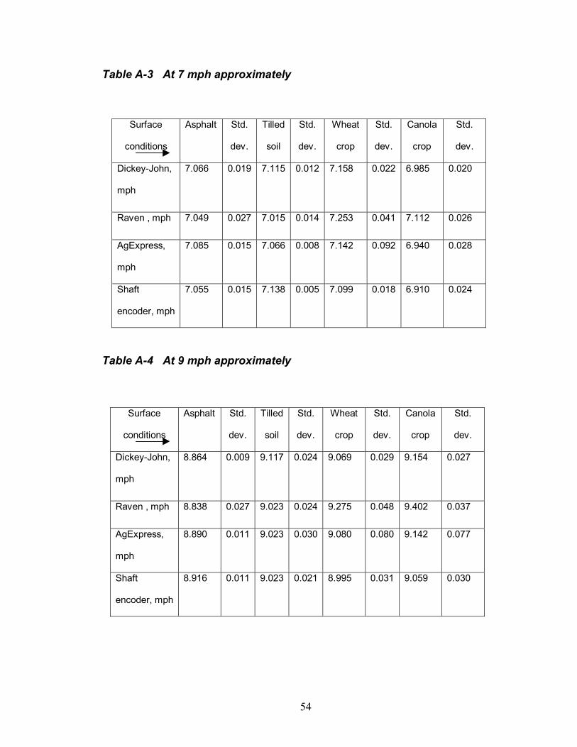
Table A-3 At 7 mph approximately
Table A-4 At 9 mph approximately
Surface
conditions
Asphalt Std.
dev.
Tilled
soil
Std.
dev.
Wheat
crop
Std.
dev.
Canola
crop
Std.
dev.
Dickey-John,
mph
7.066 0.019 7.115 0.012 7.158 0.022 6.985 0.020
Raven , mph 7.049 0.027 7.015 0.014 7.253 0.041 7.112 0.026
AgExpress,
mph
7.085 0.015 7.066 0.008 7.142 0.092 6.940 0.028
Shaft
encoder, mph
7.055 0.015 7.138 0.005 7.099 0.018 6.910 0.024
Surface
conditions
Asphalt Std.
dev.
Tilled
soil
Std.
dev.
Wheat
crop
Std.
dev.
Canola
crop
Std.
dev.
Dickey-John,
mph
8.864 0.009 9.117 0.024 9.069 0.029 9.154 0.027
Raven , mph 8.838 0.027 9.023 0.024 9.275 0.048 9.402 0.037
AgExpress,
mph
8.890 0.011 9.023 0.030 9.080 0.080 9.142 0.077
Shaft
encoder, mph
8.916 0.011 9.023 0.021 8.995 0.031 9.059 0.030

55
Table A-5 ANOVA table for asphalt surface
Source DF SS MS F Pr > F
Model 15 460.308 30.687 132106 < 0.0001
Error 80 0.0186 0.0002
Corrected Total 95 460.326
Source DF Anova SS Mean Square F Value Pr > F speed 3 460.2388607 153.4129536 660432 <.0001 sensor 3 0.0029964 0.0009988 4.30 0.0073 speed*sensor 9 0.0662213 0.0073579 31.68 <.0001
Table A-6 ANOVA for canola surface
Source DF SS MS F Pr > F
Model 15 499.837 33.322 26231.2 < 0.0001
Error 80 0.1016 0.0013
Corrected Total 95 499.938
Source DF Anova SS Mean Square F Value Pr > F speed 3 499.1443652 166.3814551 130974 <.0001 sensor 3 0.5950839 0.1983613 156.15 <.0001 speed*sensor 9 0.0976021 0.0108447 8.54 <.0001
56
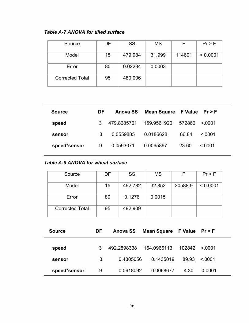
Table A-7 ANOVA for tilled surface
Source DF SS MS F Pr > F
Model 15 479.984 31.999 114601 < 0.0001
Error 80 0.02234 0.0003
Corrected Total 95 480.006
Source DF Anova SS Mean Square F Value Pr > F speed 3 479.8685761 159.9561920 572866 <.0001 sensor 3 0.0559885 0.0186628 66.84 <.0001 speed*sensor 9 0.0593071 0.0065897 23.60 <.0001
Table A-8 ANOVA for wheat surface
Source DF SS MS F Pr > F
Model 15 492.782 32.852 20588.9 < 0.0001
Error 80 0.1276 0.0015
Corrected Total 95 492.909
Source DF Anova SS Mean Square F Value Pr > F
speed 3 492.2898338 164.0966113 102842 <.0001 sensor 3 0.4305056 0.1435019 89.93 <.0001 speed*sensor 9 0.0618092 0.0068677 4.30 0.0001

57
77.17.27.37.47.57.67.77.87.9
88.18.28.38.48.58.68.78.88.9
9
1 11 21 31 41 51 61 71 81 91 101 111
time, sec.
spee
d, k
mph
GVS
Shaft encoder
Dickey-John
Raven
Appendix B
Figure B-1 Graph depicting speed vs. time on asphalt surface at 5 kmph
Figure B-2 Graph depicting speed vs. time on asphalt surface at 8 kmph
44.14.24.34.44.54.64.74.84.9
55.15.25.35.45.55.65.75.8
1 11 21 31 41 51 61 71 81 91 101
111
121
131
141
151
161
171
181
191
time, sec.
spee
d, k
mph
GVS
Shaft encoder
Dickey-John
Raven
58
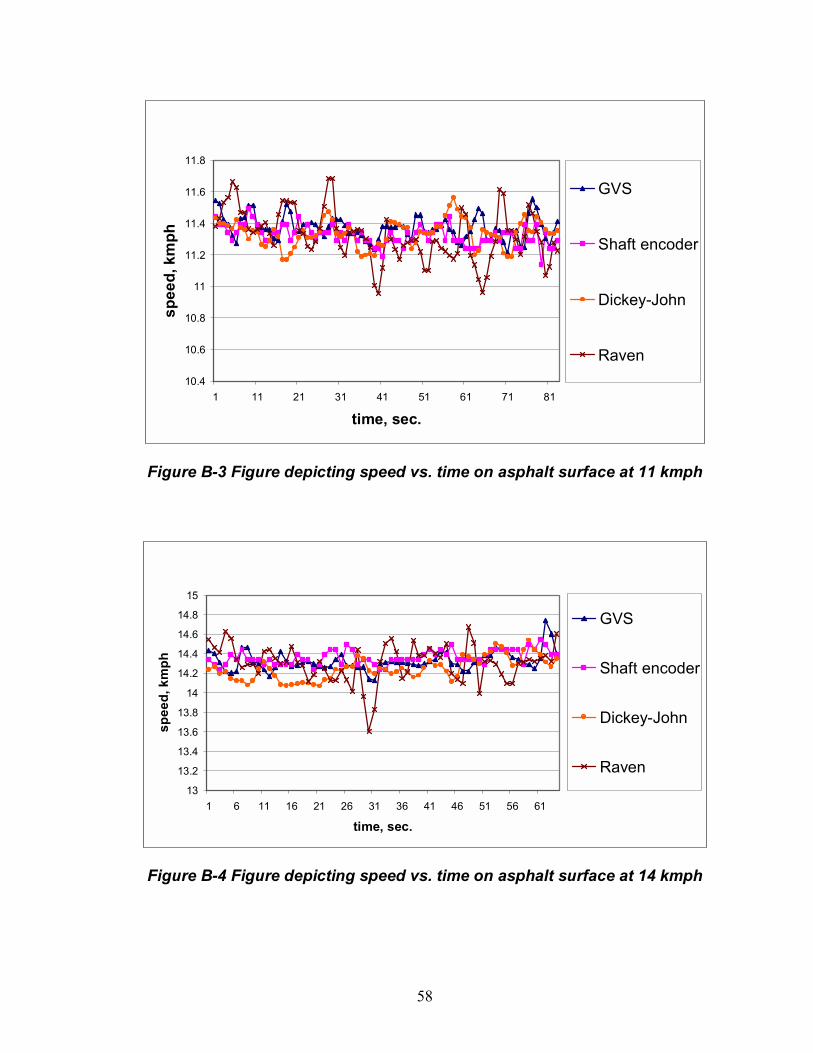
Figure B-3 Figure depicting speed vs. time on asphalt surface at 11 kmph
Figure B-4 Figure depicting speed vs. time on asphalt surface at 14 kmph
10.4
10.6
10.8
11
11.2
11.4
11.6
11.8
1 11 21 31 41 51 61 71 81
time, sec.
spee
d, k
mph
GVS
Shaft encoder
Dickey-John
Raven
13
13.2
13.4
13.6
13.8
14
14.2
14.4
14.6
14.8
15
1 6 11 16 21 26 31 36 41 46 51 56 61
time, sec.
spee
d, k
mph
GVS
Shaft encoder
Dickey-John
Raven
59
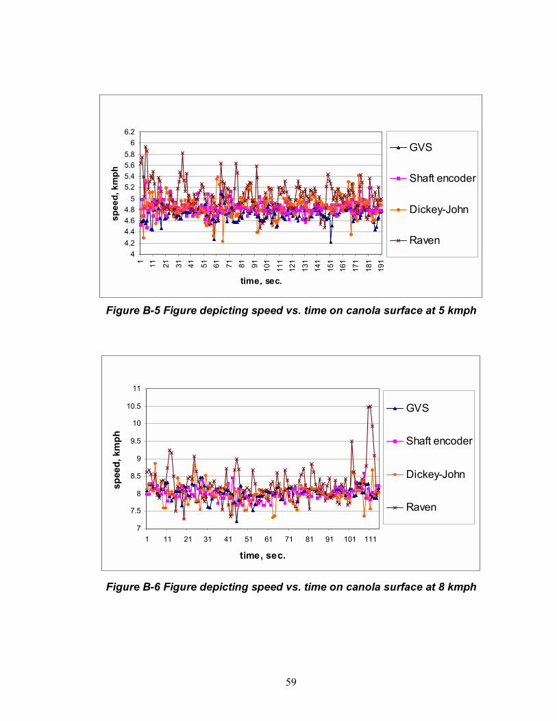
Figure B-5 Figure depicting speed vs. time on canola surface at 5 kmph
Figure B-6 Figure depicting speed vs. time on canola surface at 8 kmph
7
7.5
8
8.5
9
9.5
10
10.5
11
1 11 21 31 41 51 61 71 81 91 101 111
time, sec.
spee
d, k
mph
GVS
Shaft encoder
Dickey-John
Raven
44.24.44.64.8
55.25.45.65.8
66.2
1 11 21 31 41 51 61 71 81 91 101
111
121
131
141
151
161
171
181
191
time, sec.
spee
d, k
mph
GVS
Shaft encoder
Dickey-John
Raven
60
9
9.5
10
10.5
11
11.5
12
12.5
13
1 6 11 16 21 26 31 36 41 46 51 56 61 66 71 76 81
time, sec.
spee
d, k
mph
GVS
Shaft encoder
Dickey-John
Raven
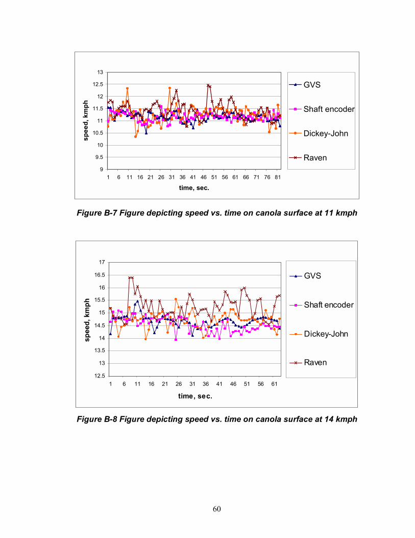
Figure B-7 Figure depicting speed vs. time on canola surface at 11 kmph
Figure B-8 Figure depicting speed vs. time on canola surface at 14 kmph
12.5
13
13.5
14
14.5
15
15.5
16
16.5
17
1 6 11 16 21 26 31 36 41 46 51 56 61
time, sec.
spee
d, k
mph
GVS
Shaft encoder
Dickey-John
Raven
61
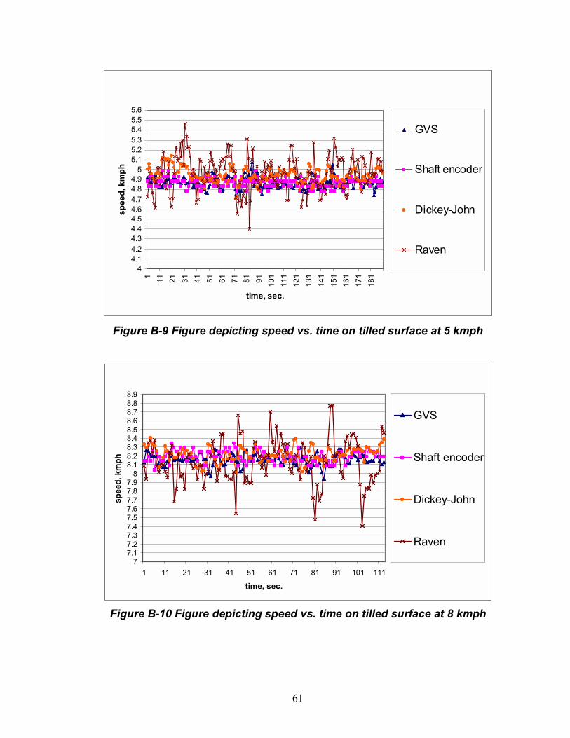
Figure B-9 Figure depicting speed vs. time on tilled surface at 5 kmph
Figure B-10 Figure depicting speed vs. time on tilled surface at 8 kmph
44.14.24.34.44.54.64.74.84.9
55.15.25.35.45.55.6
1 11 21 31 41 51 61 71 81 91 101
111
121
131
141
151
161
171
181
time, sec.
spee
d, k
mph
GVS
Shaft encoder
Dickey-John
Raven
77.17.27.37.47.57.67.77.87.9
88.18.28.38.48.58.68.78.88.9
1 11 21 31 41 51 61 71 81 91 101 111
time, sec.
spee
d, k
mph
GVS
Shaft encoder
Dickey-John
Raven
62
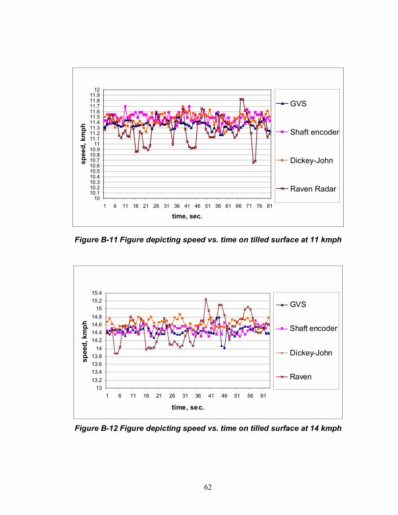
Figure B-11 Figure depicting speed vs. time on tilled surface at 11 kmph
Figure B-12 Figure depicting speed vs. time on tilled surface at 14 kmph
1010.110.210.310.410.510.610.710.810.9
1111.111.211.311.411.511.611.711.811.9
12
1 6 11 16 21 26 31 36 41 46 51 56 61 66 71 76 81
time, sec.
spee
d, k
mph
GVS
Shaft encoder
Dickey-John
Raven Radar
1313.213.413.613.8
1414.214.414.614.8
1515.215.4
1 6 11 16 21 26 31 36 41 46 51 56 61
time, sec.
spee
d, k
mph
GVS
Shaft encoder
Dickey-John
Raven

63
Figure B-13 Figure depicting speed vs. time on wheat surface at 5 kmph
Figure B-14 Figure depicting speed vs. time on wheat surface at 8 kmph
4
4.2
4.4
4.6
4.8
5
5.2
5.4
5.6
5.8
61 11 21 31 41 51 61 71 81 91 101
111
121
131
141
151
161
171
181
191
time, sec.
spee
d, k
mph
GVS
Shaft encoder
Dickey-John
Raven
4
4.2
4.4
4.6
4.8
5
5.2
5.4
5.6
5.8
6
6.2
1 11 21 31 41 51 61 71 81 91 101 111
time, sec.
spee
d, m
ph
GVS
Shaftencoder
Dickey-John
Raven
64
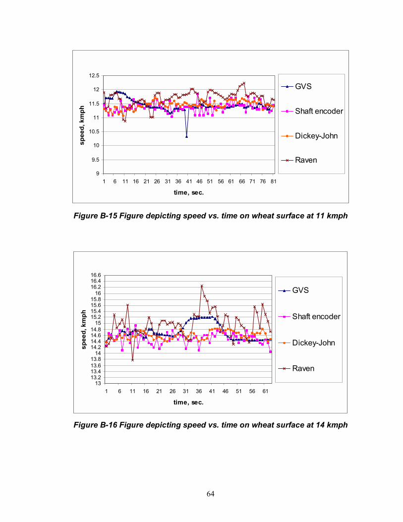
Figure B-15 Figure depicting speed vs. time on wheat surface at 11 kmph
Figure B-16 Figure depicting speed vs. time on wheat surface at 14 kmph
9
9.5
10
10.5
11
11.5
12
12.5
1 6 11 16 21 26 31 36 41 46 51 56 61 66 71 76 81
time, sec.
spee
d, k
mph
GVS
Shaft encoder
Dickey-John
Raven
1313.213.413.613.8
1414.214.414.614.8
1515.215.415.615.8
1616.216.416.6
1 6 11 16 21 26 31 36 41 46 51 56 61
time, sec.
spee
d, k
mph
GVS
Shaft encoder
Dickey-John
Raven

65
Figure B-17 Speed Vs. Time on canola surface during acceleration
Figure B-18 Speed, Error Vs. Time on canola surface during acceleration
0
5
10
15
20
25
1 5 9 13 17 21 25 29 33 37 41 45 49 53 57 61
time, sec.
spee
d, k
mph
GVS
Shaft Encoder
Dickey-John
Raven
0 1 2 3 4 5 6 7 8-5
-4
-3
-2
-1
0
1
2
time, sec.
erro
r, km
ph
05
10
15
20
spee
d, k
mph
GVSDickey-JohnRaven
Predicted velocity (SE)
66
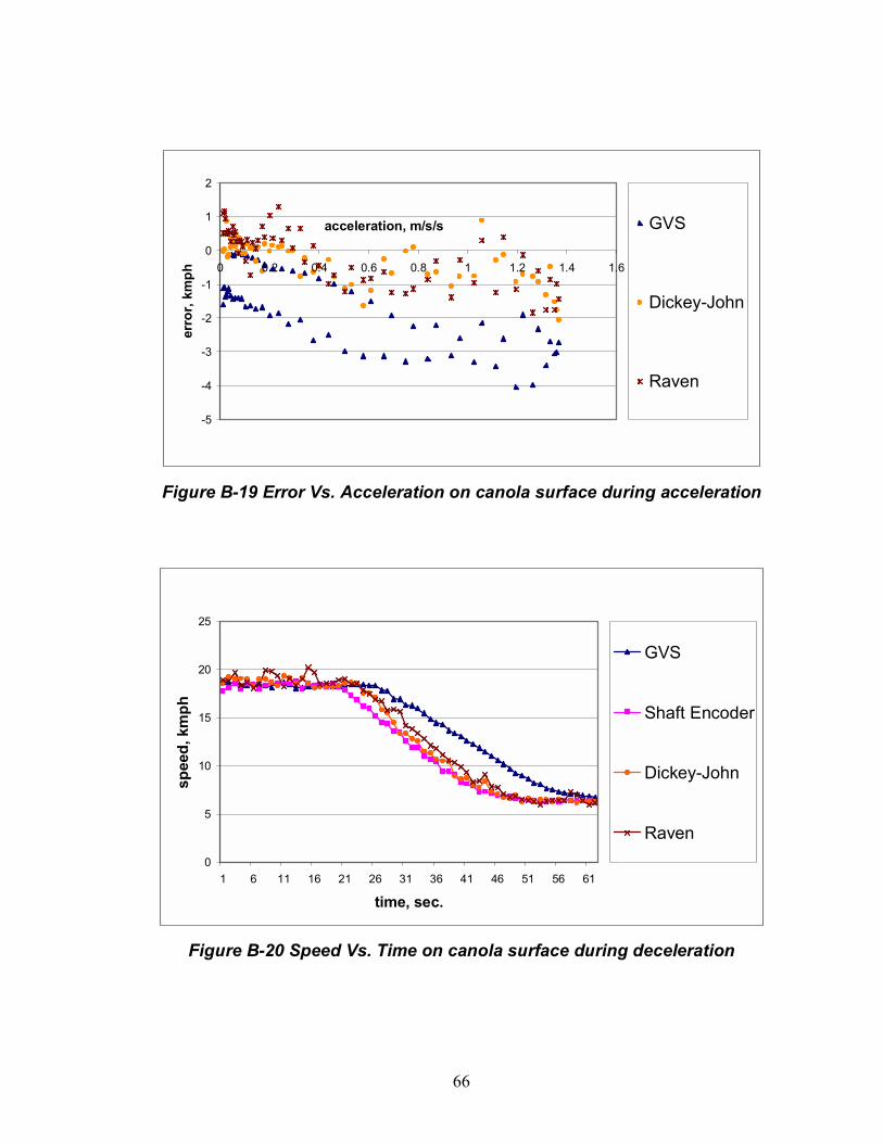
Figure B-19 Error Vs. Acceleration on canola surface during acceleration
Figure B-20 Speed Vs. Time on canola surface during deceleration
0
5
10
15
20
25
1 6 11 16 21 26 31 36 41 46 51 56 61
time, sec.
spee
d, k
mph
GVS
Shaft Encoder
Dickey-John
Raven
-5
-4
-3
-2
-1
0
1
2
0 0.2 0.4 0.6 0.8 1 1.2 1.4 1.6
acceleration, m/s/s
erro
r, km
ph
GVS
Dickey-John
Raven
67
Error Vs. Deceleration on canola surface
-0.5
0
0.5
1
1.5
2
2.5
3
3.5
-3.5 -3 -2.5 -2 -1.5 -1 -0.5 0
deceleration, m/h/h
erro
r, m
ph
GVS
Dickey-John
Raven
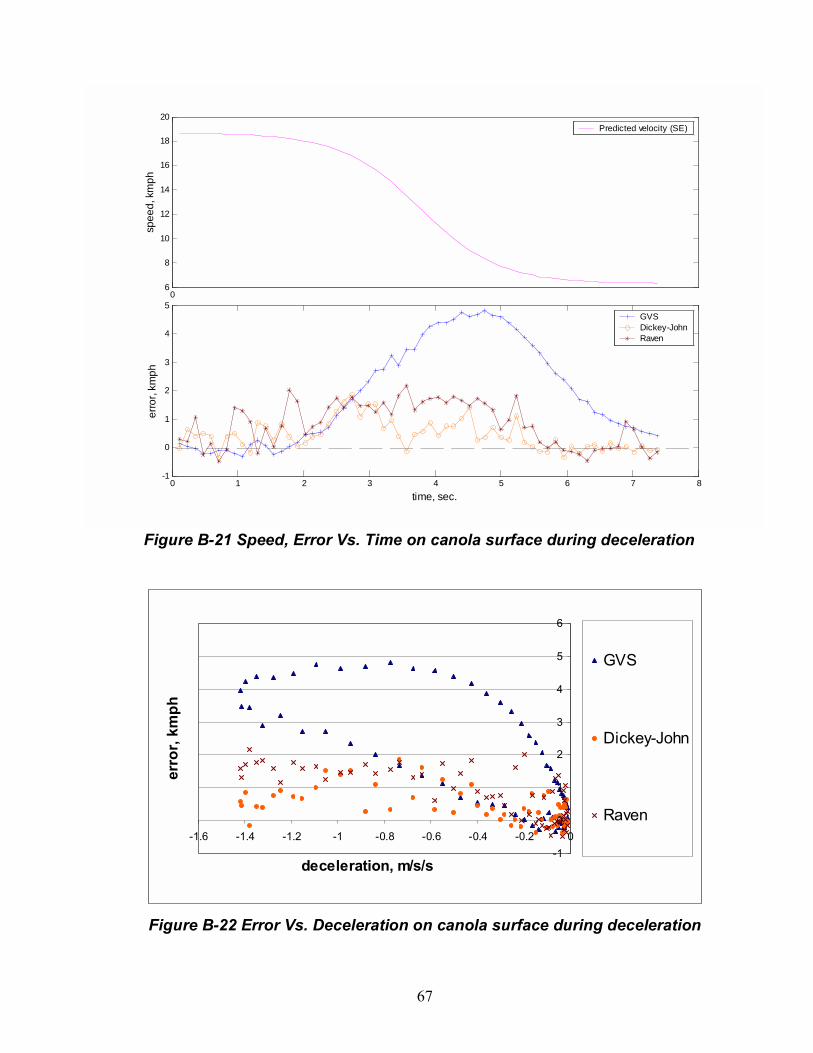
Figure B-21 Speed, Error Vs. Time on canola surface during deceleration
Figure B-22 Error Vs. Deceleration on canola surface during deceleration
06
8
10
12
14
16
18
20
spee
d, k
mph
0 1 2 3 4 5 6 7 8-1
0
1
2
3
4
5
time, sec.
erro
r, km
ph
Predicted velocity (SE)
GVSDickey-JohnRaven
-1
0
1
2
3
4
5
6
-1.6 -1.4 -1.2 -1 -0.8 -0.6 -0.4 -0.2 0
deceleration, m/s/s
erro
r, km
ph
GVS
Dickey-John
Raven

68
Figure B-23 Speed Vs. Time on wheat surface during acceleration
Figure B-24 Speed, Error Vs. Time on wheat surface during acceleration
0
5
10
15
20
25
1 6 11 16 21 26 31 36 41 46 51 56
time, sec.
spee
d, m
ph
GVS
Shaft Encoder
Dickey-John
Raven
05
10
15
20
spee
d, k
mph
0 1 2 3 4 5 6 7-5
-4
-3
-2
-1
0
1
2
time, sec.
erro
r, km
ph
GVSDickey-JohnRaven
Predicted velocity (SE)
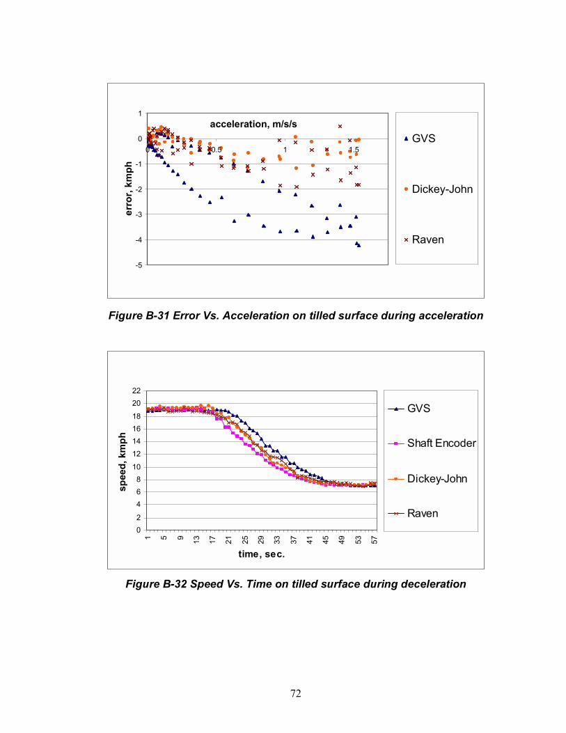
69
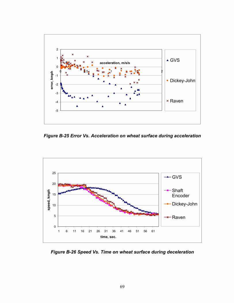
Figure B-25 Error Vs. Acceleration on wheat surface during acceleration
Figure B-26 Speed Vs. Time on wheat surface during deceleration
0
5
10
15
20
25
1 6 11 16 21 26 31 36 41 46 51 56 61
time, sec.
spee
d, k
mph
GVS
ShaftEncoder
Dickey-John
Raven
-5
-4
-3
-2
-1
0
1
2
0 0.5 1 1.5 2
acceleration, m/s/s
erro
r, km
ph
GVS
Dickey-John
Raven
70
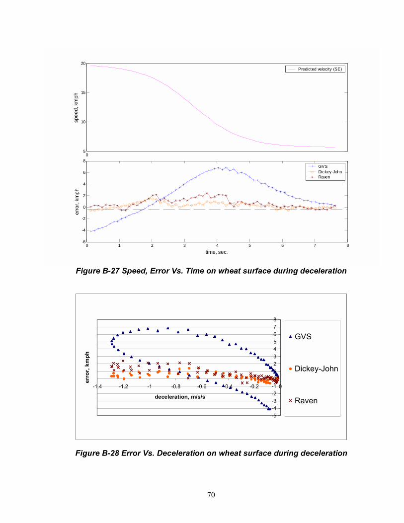
Figure B-27 Speed, Error Vs. Time on wheat surface during deceleration
Figure B-28 Error Vs. Deceleration on wheat surface during deceleration
05
10
15
20
spee
d, k
mph
0 1 2 3 4 5 6 7 8-6
-4
-2
0
2
4
6
8
erro
r, km
ph
time, sec.
Predicted velocity (SE)
GVSDickey-JohnRaven
-5-4-3-2-1012345678
-1.4 -1.2 -1 -0.8 -0.6 -0.4 -0.2 0
deceleration, m/s/s
erro
r, km
ph
GVS
Dickey-John
Raven
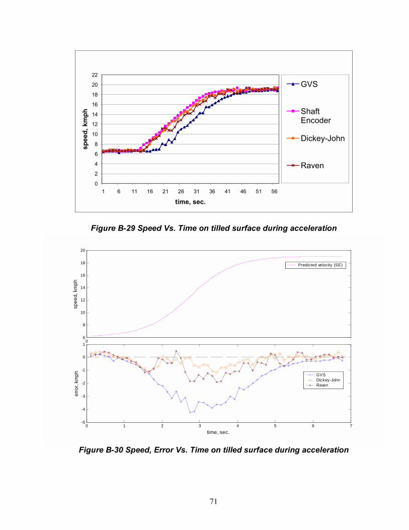
71
Figure B-29 Speed Vs. Time on tilled surface during acceleration
Figure B-30 Speed, Error Vs. Time on tilled surface during acceleration
0
2
4
6
8
10
12
14
16
18
20
22
1 6 11 16 21 26 31 36 41 46 51 56
time, sec.
spee
d, k
mph
GVS
ShaftEncoder
Dickey-John
Raven
0 1 2 3 4 5 6 7-5
-4
-3
-2
-1
0
1
time, sec.
erro
r, km
ph
06
8
10
12
14
16
18
20
spee
d, k
mph
Predicted velocity (SE)
GVSDickey-JohnRaven
72
Figure B-31 Error Vs. Acceleration on tilled surface during acceleration
Figure B-32 Speed Vs. Time on tilled surface during deceleration
02
468
10
12141618
2022
1 5 9 13 17 21 25 29 33 37 41 45 49 53 57
time, sec.
spee
d, k
mph
GVS
Shaft Encoder
Dickey-John
Raven
-5
-4
-3
-2
-1
0
1
0 0.5 1 1.5
acceleration, m/s/ser
ror,
kmph
GVS
Dickey-John
Raven
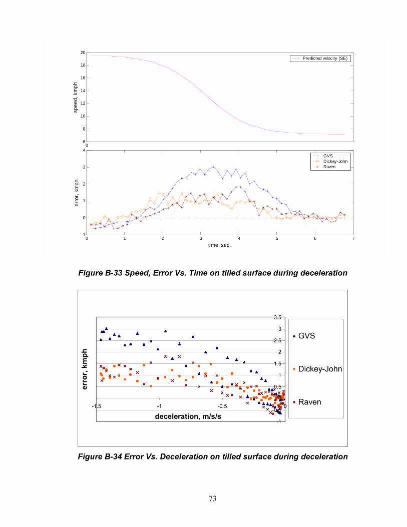
73
Figure B-33 Speed, Error Vs. Time on tilled surface during deceleration
Figure B-34 Error Vs. Deceleration on tilled surface during deceleration
06
8
10
12
14
16
18
20
spee
d, k
mph
0 1 2 3 4 5 6 7-1
0
1
2
3
4
time, sec.
erro
r, km
ph
Predicted velocity (SE)
GVSDickey-JohnRaven
-1
-0.5
0
0.5
1
1.5
2
2.5
3
3.5
-1.5 -1 -0.5 0
deceleration, m/s/s
erro
r, km
ph
GVS
Dickey-John
Raven
VITA
Ramesh Vishwanathan
Candidate for the Degree of
Master of Science
Dissertation: EVALUATION OF GROUND SPEED SENSING DEVICES UNDER VARYING GROUND SURFACE CONDITIONS
Major Field: Biosystems Engineering
Biographical:
Personal Data: Born in Madras (now Chennai), India on July 19, 1974, as son to Mr. R.Vishwanathan and Mrs. Rama Vishwanathan.
Education: Bachelor of Engineering in Agricultural Engineering from
Rajasthan Agricultural University, Rajasthan, India (1997). Completed the requirements for the Master of Science degree with major in Biosystems and Agricultural Engineering at Oklahoma State University, July, 2005.
Experience: Worked as Field Engineer in Rajasthan Agriculture Drainage
research project, Rajasthan, India (1997-1999). Worked for Tractor and Farm Equipment Limited (TAFE), Chennai, India (1999-2003). Graduate Research Assistant at Biosystems Engineering department, Oklahoma State University, Stillwater, OK (Aug 2003-July 2005).
Professional Memberships: American Society of Agricultural Engineers
(ASAE).
Name: Ramesh Vishwanathan Date of Degree: July, 2005
Institution: Oklahoma State University Location: Stillwater, Oklahoma
Title of Study: EVALUATION OF GROUND SPEED SENSING DEVICES UNDER VARYING GROUND SURFACE CONDITIONS
Pages in Study: 73 Candidate for Degree of Master of Science
Major Field: Biosystems Engineering
Abstract: The objective of this study was to compare several commercially available
methods of ground speed measurement under varying vegetative covers and
ground conditions. Empirical field observations indicated that radar ground speed
measurements show increased error as crop vegetative cover/ height increases.
A low cost GPS based ground velocity sensor has been recently developed, and
that system was compared to the other speed sensors as well. These systems
were compared to a reference (true) ground speed. The experimental study
included instrumentation of a tractor with speed sensors and a data acquisition
system.
Findings and Conclusions:
GPS based velocity sensor can be an inexpensive alternative to radar
sensors for steady state applications, however further refinements in the system
are required for its intended use in transient speed conditions. The speed
measurements obtained from radar sensors were within the acceptable accuracy
range, although further refinements in Raven radar data are necessary to make it
insensitive towards canopy effect of the crops. Results included validation of
GPS and radar sensors for true ground speed measurements in terms of their
accuracy and reliability.
Advisor�s Approval: __________Dr. Paul R. Weckler_______________________