Evaluation of Features Detectors and Descriptors based on 3D objects

Pierre Moreels and Pietro PeronaCalifornia Institute of Technology, Pasadena CA91125, USA

Abstract

We explore the performance of a number of popular fea-ture detectors and descriptors in matching 3D object fea-tures across viewpoints and lighting conditions. To this endwe design a method, based on intersecting epipolar con-straints, for providing ground truth correspondence auto-matically. We collect a database of 100 objects viewed from144 calibrated viewpoints under three different lightingconditions. We find that the combination of Hessian-affinefeature finder and SIFT features is most robust to viewpointchange. Harris-affine combined with SIFT and Hessian-affine combined with shape context descriptors were best re-spectively for lighting changes and scale changes. We alsofind that no detector-descriptor combination performs wellwith viewpoint changes of more than 25-30◦.

1 Introduction

Detecting and matching specific visual features across dif-ferent images has been shown to be useful for a diverseset of visual tasks including stereoscopic vision [1, 2],vision-based simultaneous localization and mapping for au-tonomous vehicles [3], mosaicking images [4] and recog-nizing objects [5, 6]. This operation typically involves threedistinct steps. First a ‘feature detector’ identifies a set of im-age locations presenting rich visual information and whosespatial location is well defined. The spatial extent or ‘scale’of the feature may also be identified in this first step. Thesecond step is ‘description’: a vector characterizing localtexture is computed from the image near the nominal lo-cation of the feature. ‘Matching’ is the third step: a givenfeature is associated with one or more features in other im-ages. Important aspects of matching are metrics and criteriato decide whether two features should be associated, anddata structures and algorithms for matching efficiently.

The ideal system will be able to detect a large numberof meaningful features in the typical image, and will matchthem reliably across different views of the same scene / ob-ject. Critical issues in detection, description and match-ing are robustness with respect to viewpoint and lightingchanges, the number of features detected in a typical im-age, the frequency of false alarms and mismatches, and

Figure 1: (top row) Large (≈ 50◦) viewpoint change for a flatscene. Many interest points can be matched after the transforma-tion - images courtesy of K.Mikolajczyk - the appearance changeis modeled by an affine transformation. (bottom row) Similarviewpoint change for a 3D scene. Many visually salient featuresare associated with locations where the 3D surface is irregular ornear boundaries, the change in appearance of these features withthe viewing direction is not easy to model.

the computational cost of each step. Different applica-tions weigh these requirements differently. For example,viewpoint changes more significantly in object recognition,SLAM and wide-baseline stereo than in image mosaicking,while the frequency of false matches may be more critical inobject recognition, where thousands of potentially matchingimages are considered, rather than in wide-baseline stereoand mosaicing where only few images are present.

A number of different feature detectors [2, 7, 8, 9, 10,11], feature descriptors [6, 12, 13, 14] and feature match-ers [5, 6, 15, 16] have been proposed in the literature. Theycan be variously combined and concatenated to producedifferent systems. Which combination should be used ina given application? A couple of studies are available.Schmid [5] characterized and compared the performanceof several features detectors. Recently, Mikolajczik andSchmid [17] focused primarily on the descriptor stage. For achosen detector, the performance of a number of descriptorswas assessed. These evaluations of interest point operatorsand feature descriptors, have relied on the use of flat images,or in some cases synthetic images. The reason is that thetransformation between pairs of images can be computed

1

Figure 2: Our calibrated database consists of photographs of 100 objects which were imaged in three lighting conditions: diffuse lighting,light from left and light from right. We chose our objects to represent a wide variety of shapes and surface properties. Each objectwas photographed by two cameras located above each over, 10◦ apart.(Top) Eight sample objects from our collection. (Bottom) Eachobject was rotated with 5◦ increments and photographed at each orientation with both cameras and three lighting conditions for a total of72 × 2 × 3 = 432 photographs per object. Eight such photographs are shown for one of our objects.

easily, which is convenient to establish ground truth.However, the relative performance of various detectors

can change when switching from planar scenes to 3D im-ages (see Fig. 12 and [18]). Features detected in an im-age are generated in part by texture, and in part by the geo-metric shape of the object. Features due to texture are flat,lie far from object boundaries and exhibit a high stabilityacross viewpoints [5, 17]. Features due to shape are foundnear edges, corners and folds of the object. Due to self-occlusions, they have a much lower stability with respectto viewpoint change. These features due to shape, or 3Dfeatures, represent a large fraction of all detected features.

The present study is complementary to those from [5,14, 17, 18]. We evaluate the performance of feature detec-tors and descriptors for images of 3D objects viewed underdifferent viewpoint, lighting and scale conditions. To thiseffect, we collected a database of 100 objects viewed from144 different calibrated viewpoints under 3 lighting condi-tions. We also developed a practical and accurate methodfor establishing automatically ground truth in images of 3Dscenes. Unlike [18] ground truth is established using geo-metric constraints only, so that the feature/descriptor eval-uation is not biased by an early use of conditions on ap-pearance matches. Besides, our method is fully automated,so that the evaluation can be performed on a large-scaledatabase, rather than on a handful of images as in [17, 18].

Another novel aspect is the use of a metric for accept-ing/rejecting feature matches due to D. Lowe [6]; it is basedon the ratio of the distance of a given feature from its bestmatch vs the distance to the second best match. This met-ric has been shown to perform better than the traditionaldistance-to-best-match.

In section 2 we describe the geometrical considerationswhich allow us to construct automatically a ground truth forour experiments. In section 3 we describe our laboratorysetup and the database of images we collected. Section 4describes the decision process used in order to assess per-formances of detectors and descriptors. Section 5 presentsthe experiments. Section 6 contains our conclusions.

2 Ground truthIn order to evaluate a particular detector-descriptor combi-nation we need to calculate the probability that a feature ex-tracted in a given image, can be matched to the correspond-ing feature in an image of the same object/scene viewedfrom a different viewpoint. For this to succeed, the physicallocation must be visible in both images, the feature detectormust detect it in both cases with minimal positional varia-tion, and the descriptor of the features must be sufficientlyclose. To compute this probability we must be able to tell ifany tentative match between two features is correct or not.Conversely, whenever a feature is detected in one image, wemust be able to tell whether in the corresponding location inanother image a feature was detected and matched.

We establish ground truth by using epipolar constraintsbetween triplets of calibrated views of the objects (this isan alternative to using the trifocal tensor [19]). We distin-guish between a ‘reference’ view (A in Fig. 3) a ‘test’ viewC, and an ‘auxiliary’ view B. Given one feature f A in thereference image, any feature in C matching the referencefeature must satisfy the constraint of belonging to the cor-responding ‘reference’ epipolar line. This excludes mostpotential matches but not all of them (in our experiments,typically 0-5 features remain out of 300-600). We make thetest more stringent by imposing a second constraint. Anepipolar line lB is associated to the reference feature in theauxiliary image B. Again, f A has typically 5-10 potentialmatches along lB, each of which in turn generates an ‘aux-iliary’ epipolar line in C. The intersection of the primaryand auxiliary epipolar lines in C identify a small matchingregions, in which statistically only zero or one features aredetected.

Note that the geometry of our acquisition system (Fig. 3& Fig. 4) does not allow the degenerated case where thereference point is on the trifocal plane and both epipolarconstraints are superposed.

The benefit of using the double epipolar constraint in thetest image is that any correspondence - or lack thereof - may

2

Figure 3: Example of matching process for one feature.

be validated with extremely low error margins. The costis that only a fraction (50-70%) of the reference featureshave a correspondence in the auxiliary image, thus limitingthe number of features triplets that can be formed. If wecall pfA(θ) the probability that, given a reference featurefA, a match will exist in a view of the same scene takenfrom a viewpoint θ degrees apart, the triplet (f A, fB, fC)exists with probability pfA(θAC) · pfB (θAB), while thepair (fA, fC) exists with higher probability pfA(θAC).While the measurements we take allow for a relative assess-ment of different methods, they should be renormalized by1/pfA(θAB) to obtain absolute performance figures.

3 Experimental setup

3.1 Photographic setup and database

Our acquisition system consists of 2 cameras taking pic-tures of objects on a motorized turntable (see Fig. 4). Thechange in viewpoint is performed by the rotation of theturntable. The lower camera takes the reference view, thenthe turntable is rotated and the same camera takes the testview. Each acquisition was repeated with 3 lighting con-ditions obtained with a set of photographic spotlights anddiffusers.

The database consisted of 100 different objects. Fig. 2shows some examples from this databaset. Most ob-jects were 3-dimensional, with folds and self-occlusions,which are a major cause of features instability in real-worldscenes, as opposed to 2D objects. We included some flatobjects (e.g. box of cereals). The database contains bothtextured objects (pineapple, globe) and objects with a morehomogenous surface (bananas, horse).

3.2 Calibration

The calibration images were acquired using a checkerboardpattern. Both cameras were automatically calibrated usingthe calibration routines in Intel’s Open CV library [20].

Figure 4: (Top) Photograph of our laboratory setup. Each ob-ject was placed on a computer-controlled turntable which can berotated with 1/50 degree resolution and 10−5 degree accuracy.Two computer-controlled cameras imaged the object. The cameraswere located 10◦ apart with respect to the object. The resolutionis 4Mpixels. (Bottom) Diagram explaining the geometry of ourthree-cameras arrangement and of the triple epipolar constraint.

Uncertainty on the position of the epipolar lines positionwas estimated by Monte Carlo perturbations of the calibra-tion patterns. Hartley & Zisserman [21] showed that theenvelope of the epipolar lines obtained when the fundamen-tal matrix varies around its mean value, is a hyperbola. Thecalibration patterns were perturbed randomly by up to 5 pix-els. This quantity was chosen so that it would produce areprojection error on the grid’s corners that was comparableto the one observed during calibration. This was followedby the calibration optimization.

For each point P of the first image, the Monte-Carlo pro-cess leads to a bundle of epipolar lines in the second image,whose envelope is the hyperbola of interest. The width be-tween the two branches of the hyperbola varied between 3and 5 pixels. The area inside the hyperbola defines the re-gion allowed for detection of a match to P .

3.3 Detectors and descriptors

3.3.1 Detectors

- The Harris detector [7] relies on first order derivatives ofthe image intensities. It it based on the second order mo-ment matrix (or squared gradient matrix).- The Hessian detector [8] is a second order filter. The cor-ner strength is here the negative determinant of the matrixof second order derivatives.- Affine-invariant versions of the previous two detectors

3

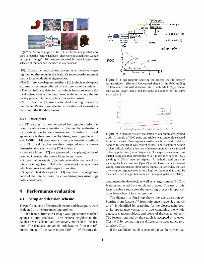
Figure 5: A few examples of the 535 irrelevant images that wereused to load the feature database. They were obtained from Googleby typing ‘things’. 105 features detected in these images wereselected at random and included in our database

[10]. The affine rectification process is an iterative warp-ing method that reduces the feature’s second-order momentmatrix to have identical eigenvalues.- The Difference-of-gaussian filters [11] selects scale-spaceextrema of the image filtered by a difference of gaussians.- The Kadir-Brady detector [9] selects locations where thelocal entropy has a maximum over scale and where the in-tensity probability density function varies fastest.- MSER features [2] use a watershed flooding process onthe image. Regions are selected at locations of slowest ex-pansion of the flooding basins.

3.3.2 Descriptors

- SIFT features [6] are computed from gradient informa-tion. Invariance to orientation is obtained by evaluating amain orientation for each feature and offsetting it. Localappearance is then described by histograms of gradients.- PCA-SIFT [14] computes a primary orientation similarlyto SIFT. Local patches are then projected onto a lower-dimensional space by using PCA analysis.- Steerable filters [12] are generated by applying banks oforiented Gaussian derivative filters to an image.- Differential invariants [5] combine local derivatives of theintensity image (up to 3rd order derivative) into quantitieswhich are invariant with respect to rotation.- Shape context descriptors [13] represent the neighbor-hood of the interest point by color histograms using log-polar coordinates.

4 Performance evaluation

4.1 Setup and decision scheme

The performances of features detectors and descriptors wereevaluated on a feature matching problem.

Each feature from a test image was appearance-matchedagainst a large database. The nearest neighbor in thisdatabase was selected and tentatively matched to the fea-ture. The database contained both features from one ref-erence image of the same object (102 − 103 features de-

Figure 6: (Top) Diagram showing the process used to classifyfeature triplets. (Bottom) Conceptual shape of the ROC tradingoff false alarm rate with detection rate. The threshold Tapp cannottake values larger than 1 and the ROC is bounded by the curvep1 + p2 = 1.

2 3 4 5 6 7 8 9 10 110

0.1

0.2

0.3

0.4

0.5

threshold (pixels) on distance allowed from features to epipolar lines

erro

r ra

te

pairs

triplets

pairs − triplets

Figure 7: Operator-assisted validation of our automated groundtruth. A sample of 3000 pairs and triplets was randomly selectedfrom our dataset. Two experts classified each pair and triplet byhand as to whether it was correct or not. The fraction of wrongtriplets is displayed as a function of the maximum distance allowedto the epipolar line (curve ‘triplets’). Our experiments were con-ducted using adaptive thresholds of 3-5 pixels (see section 3.2),yielding ≈ 2% of incorrect triplets. A method based on a sin-gle epipolar line constraint (‘pairs’) would have entailed a rate ofwrong correspondences three times higher. In particular, the rateof wrong correspondences is very high for features that could bematched in two images but not in all 3 images (‘pairs − triplets’).

pending on the detector), as well as a large number (10 5) offeatures extracted from unrelated images. The use of thislarge database replicates the matching process in applica-tions from object/class recognition.

The diagram in Fig.6-top shows the decision strategy.Starting from feature f A from reference image A, a matchto fA is identified by searching for the closest neighbourto its appearance vector, in a tree containing the wholedatabase (random objects and views of the correct object).The feature returned by the search is accepted or rejected(Test #1) by comparing the difference in appearance to athreshold Tapp.

If the candidate match is accepted, it can be correct, i.e.

4

correspond to the same physical point, or incorrect. If itcomes from a wrong image (Test #2), it is incorrect. Ifit comes from a view of the correct object, we use epipo-lar constraints (Test #3) with the following method (Fig.4-(bottom)). Starting from feature f A in reference image A,candidate matches are identified along the correspondingepipolar line in the auxiliary image B. Besides, the ob-ject lies on the turntable which has a known depth, so thatonly a known region on the epipolar line is allowed. Thereremains n candidate matches f B1 ...fBn in B (typically 0-5points). These points generate epipolar lines in the test im-age C, which intersect the epipolar line from f A at pointsfC1...fCn . If the candidate match is one of these points wedeclare it as a correct match, in the alternative it is consid-ered incorrect (false alarm).

In case no feature was found along the epipolar line inthe auxiliary image B, the initial point f A is discarded anddoesn’t contribute to any statistics, since our inability to es-tablish a triple match is not caused by a poor performanceof the detector on the target image C.

Note that this method doesn’t guarantee the absence offalse alarms. But it offers the important advantage of beingpurely geometric. Any method involving appearance vec-tors as an additional constraint would be dependent on theunderlying descriptor and bias our evaluation.

In order to evaluate the fraction of wrong correspon-dences established by our geometric system, 2 users exam-ined visually random triplets accepted by the system andclassified them into correct and incorrect matches. 3000matches were examined, results are reported in Fig.7(right).The users also classified matches obtained by a simplermethod that uses only the reference and test views of theobject and one epipolar constraint - cf. section 2 - Thefraction of wrong matches is displayed as a function of thethreshold on the maximum distance in pixels allowed be-tween features and epipolar lines. We also display the errorrate for features that could be matched using the 2-viewsmethod, but for which no triplet was identified. The methodusing 3 views shows a significantly better performance.

4.2 Distance measure in appearance space

In order to decide on acceptance or rejection of a can-didate match (first decision in Fig.6), we need a metricon appearance space. Instead of using directly the Eu-clidean/Mahalanobis distance in appearance as in [17, 14],we use the distance ratio introduced by Lowe [6].

The proposed measure compares the distances in ap-pearance of the query point to its best and second bestmatches. In Fig.6 the query feature and its best and secondbest matches are denoted by f A, fC and fC1 respectively.The criterion used is the ratio of these two distances, i.e.d(fA,fC)d(fA,fC1) . This ratio characterizes how distinctice a given

0.1 0.2 0.3 0.4 0.5 0.6 0.7 0.8 0.9 10

1

2

3

4

5

6

7

ratio (dist. to nearest neighbour / dist. to 2nd nearest neighbour)

p(ra

tio)

correct matcheswrong matches

Figure 8: Sample pdf of the distance ratio between best andsecond best match for correct correspondences (green) and falsealarms (red). These curves are analogous to the ones in Fig.11of Lowe [6]. Lowe’s correct-match density is peaked around 0.4while ours is flat – this may be due to the fact that we use 3Dobjects, while D.Lowe uses flat images with added noise.

feature is, and avoids ambiguous matches. A low valuemeans that the best match performs significantly better thanits best contender, and is thus a reliable match. A high valueof the distance ratio is obtained when the features points areclustered in a tight group in appearance space. Those fea-tures are not distinctive enough relatively to each other. Inorder to avoid a false alarm it is safer to reject the match.

Fig.8 shows the resulting distribution of distance ratios.The distance ratios statistics were collected while runningour matching problem. Correct matches and false alarmswere identified using the process described in 4.1.

4.3 Detection and false alarm rates

As seen in the previous section and Fig.6, the system canhave 3 outcomes. In the first case, the match is rejectedbased on appearance (probability p0). In the second case,the match is accepted based on appearance, but the ge-ometry constraints are not verified: this is a false alarm(probability p1). In the third alternative, the match veri-fies both appearance and geometric conditions, this is a cor-rect detection (probability p2). These probabilities verifyp0 +p1 +p2 = 1. The false alarm rate is further normalizedby the number of database features (105). Detection rateand false alarm rate can be written as

false alarm rate =#false alarms

#attempted matches · #database(1)

detection rate =#detections

#attempted matches(2)

5 Results and Discussion

Fig.9 shows the detection results when viewing angle wasvaried and lighting/scale was held constant. Panels a-h dis-play results when varying the feature detector for a given

5

a0 0.2 0.4 0.6 0.8 1

x 10−5

0

0.05

0.1

0.15

false alarm rate

dete

ctio

n ra

te

ROC curves for descriptor: sift

multiscale Harris / sift − 204062 features testedmultiscale Hessian / sift − 180910 features testeddiff of gaussians / sift − 256920 features testeddiff of gaussians / PCASift − 228486 features testedharris affine / sift − 85541 features testedhessian affine / sift − 194150 features testedKadir / sift − 33643 features testedmser / sift − 17798 features tested

b0 0.2 0.4 0.6 0.8 1

x 10−5

0

0.05

0.1

0.15

false alarm rate

dete

ctio

n ra

te

ROC curves for descriptor: steer. filters

multiscale Harris / steer. filters − 209896 features testedmultiscale Hessian / steer. filters − 183182 features testeddiff of gaussians / steer. filters − 265015 features testedharris affine / steer. filters − 86927 features testedhessian affine / steer. filters − 201403 features testedKadir / steer. filters − 32996 features testedmser / steer. filters − 17132 features tested

c0 0.2 0.4 0.6 0.8 1

x 10−5

0

0.05

0.1

0.15

false alarm rate

dete

ctio

n ra

te

ROC curves for descriptor: rot. invariants

multiscale Harris / rot. invariants − 211619 features testedmultiscale Hessian / rot. invariants − 185847 features testeddiff of gaussians / rot. invariants − 273937 features testedharris affine / rot. invariants − 87233 features testedhessian affine / rot. invariants − 206364 features testedKadir / rot. invariants − 32930 features testedmser / rot. invariants − 16373 features tested

d0 0.2 0.4 0.6 0.8 1

x 10−5

0

0.05

0.1

0.15

false alarm rate

dete

ctio

n ra

te

ROC curves for descriptor: shape context

multiscale Harris / shape context − 207741 features testedmultiscale Hessian / shape context − 181678 features testeddiff of gaussians / shape context − 254163 features testedharris affine / shape context − 87030 features testedhessian affine / shape context − 199695 features testedKadir / shape context − 33495 features testedmser / shape context − 18256 features tested

e −40 −30 −20 −10 0 10 20 30 400

0.2

0.4

0.6

0.8

viewpoint change (camera rotation angle in degrees)

frac

tion

of s

tabl

e ke

ypoi

nts

Stability results − descriptor: sift

multiscale Harris / siftmultiscale Hessian / siftdiff of gaussians / siftdiff of gaussians / PCASiftharris affine / sifthessian affine / siftKadir / siftmser / sift

f −40 −30 −20 −10 0 10 20 30 400

0.2

0.4

0.6

0.8

viewpoint change (camera rotation angle in degrees)

frac

tion

of s

tabl

e ke

ypoi

nts

Stability results − descriptor: steer. filters

multiscale Harris / steer. filtersmultiscale Hessian / steer. filtersdiff of gaussians / steer. filtersharris affine / steer. filtershessian affine / steer. filtersKadir / steer. filtersmser / steer. filters

g −40 −30 −20 −10 0 10 20 30 400

0.2

0.4

0.6

0.8

viewpoint change (camera rotation angle in degrees)

frac

tion

of s

tabl

e ke

ypoi

nts

Stability results − descriptor: rot. invariants

multiscale Harris / rot. invariantsmultiscale Hessian / rot. invariantsdiff of gaussians / rot. invariantsharris affine / rot. invariantshessian affine / rot. invariantsKadir / rot. invariantsmser / rot. invariants

h −40 −30 −20 −10 0 10 20 30 400

0.2

0.4

0.6

0.8

viewpoint change (camera rotation angle in degrees)

frac

tion

of s

tabl

e ke

ypoi

nts

Stability results − descriptor: shape context

multiscale Harris / shape contextmultiscale Hessian / shape contextdiff of gaussians / shape contextharris affine / shape contexthessian affine / shape contextKadir / shape contextmser / shape context

i0 0.2 0.4 0.6 0.8 1

x 10−5

0

0.05

0.1

0.15

false alarm rate

frac

tion

of s

tabl

e ke

ypoi

nts

comparative ROCs: best detector for each descriptor

diff of gaussians / PCASift − 228486 features testedhessian affine / sift − 194150 features testeddiff of gaussians / steer. filters − 265015 features testeddiff of gaussians / rot. invariants − 273937 features testedhessian affine / shape context − 199695 features tested

j−40 −30 −20 −10 0 10 20 30 400

0.2

0.4

0.6

0.8

viewpoint change (camera rotation angle in degrees)

frac

tion

of s

tabl

e ke

ypoi

nts

comparative stability: best detector for each descriptor

diff of gaussians / PCASifthessian affine / siftdiff of gaussians / steer. filtersdiff of gaussians / rot. invariantshessian affine / shape context

k−40 −30 −20 −10 0 10 20 30 400

0.1

0.2

0.3

0.4

0.5

0.6

0.7

0.8

0.9

1

viewpoint change (camera rotation angle in degrees)

frac

tion

of s

tabl

e ke

ypoi

nts

comparative stability: best detector for each descriptor

diff of gaussians / PCASifthessian affine / siftdiff of gaussians / steer. filtersdiff of gaussians / rot. invariantshessian affine / shape context

Figure 9: Performance for viewpoint change - each panel a-d shows the ROC curves for a given descriptor when varying the detector.Panels e-h show the corresponding stability rates as a function of the rotation angle. The 0◦ result is obtained with different images fromthe same location. Panels i-j show the combination of each descriptor with the detector that performed best for that descriptor. Panel k issimilar to panel j, but the database used for the search tree contained only the features extracted from the correct image (easier task).

image descriptor. Panels i-j summarize for each descrip-tor, the detector that performed best. Panels a-d display theROC curves obtained by varying the threshold Tapp in thefirst step of the matching process (threshold on distinctive-ness of the features’ appearance). The number of featurestested is displayed in the legend. Panels e-h show the de-tection rate as a function of the viewing angle for a fixedfalse alarm rate of 10−6 was chosen (one false alarm every10 attempts). This false alarm rate corresponds to differentdistance ratio thresholds for each detector / descriptor com-bination. Those thresholds varied between 0.56 and 0.70 (abit lower than the 0.8 value chosen by Lowe in [6]).

The Hessian-affine and difference-of-gaussians detectorspeformed consistently best with all descriptors. While theabsolute performance of the various detectors varies whenthey are coupled with different descriptors, their rankingsvary very little. The combination of Hessian-affine withSIFT and shape context obtained the best overall score, withthe advantage to SIFT. In our graphs the false alarm ratewas normalized by the size of the database (105) so that themaximum false alarm rate was 10−5. The PCA-SIFT de-

scriptor is only combined with difference-of-gaussians, aswas done in [14]. PCA-SIFT didn’t seem to outperformSIFT as would be expected from [14].

In the stability curves, the fraction of stable featuresdoesn’t reach 1 when θ = 0◦. This is due to several fac-tors: first, triplets can be identified only when the match tothe auxiliary image succeeds (see section 2). The 10◦ view-point change between reference and auxiliary image pre-vents a number of features to be identified in both images.

Another reason lies in the tree search. The use of a treethat contains both the correct image and a large numberof unrelated images replicates the matching process usedin recognition applications. However, since some featureshave low distinctiveness, the correct image doesn’t collectall the matches. In order to evaluate the detection dropdue to the search tree, the experiment was run again with asearch tree that contained only the features from the correctimage. Fig.9-k shows the stability results, the performanceis 10-15% higher.

A third reason is the noise present in the camera. Onrepeated images taken from the same viewpoint, this noise

6

0 0.5 1

x 10−5

0

0.05

0.1

0.15

false alarm rate

frac

tion

of s

tabl

e ke

ypoi

nts

comparative ROCs: best detector for each descriptor

diff of gaussians / PCASift − 230275 features testedhessian affine / sift − 194673 features testeddiff of gaussians / steer. filters − 262970 features testeddiff of gaussians / rot. invariants − 272387 features testedhessian affine / shape context − 69754 features tested

b −40 −30 −20 −10 0 10 20 30 400

0.2

0.4

0.6

0.8

viewpoint change (camera rotation angle in degrees)

frac

tion

of s

tabl

e ke

ypoi

nts

comparative stability: best detector for each descriptor

diff of gaussians / PCASifthessian affine / siftdiff of gaussians / steer. filtersdiff of gaussians / rot. invariantshessian affine / shape context

Figure 10: Results for viewpoint change, using the Mahalanobisdistance instead of the Euclidean distance on appearance vectors

0 0.5 1

x 10−5

0

0.1

0.2

0.3

false alarm rate

frac

tion

of s

tabl

e ke

ypoi

nts

comparative ROCs: best detector for each descriptor

diff of gaussians / PCASift − 56973 features testedharris affine / sift − 22060 features testedhessian affine / steer. filters − 50218 features testedhessian affine / rot. invariants − 50962 features testedhessian affine / shape context − 46763 features tested

0 0.5 1

x 10−5

0

0.1

0.2

0.3

0.4

0.5

false alarm rate

frac

tion

of s

tabl

e ke

ypoi

nts

comparative ROCs: best detector for each descriptor

diff of gaussians / PCASift − 12684 features testedharris affine / sift − 4249 features testedhessian affine / steer. filters − 11153 features testedhessian affine / rot. invariants − 10452 features testedhessian affine / shape context − 9835 features tested

Figure 11: (Top) ROCs for variations in lighting conditions. Re-sults are averaged over 3 lighting conditions. (Bottom) ROCs forvariations in scale.

causes 5 − 10% of the features to be unstable.Another observation concerns the dramatic drop in num-

ber of matched features with viewpoint change. For a view-point change of 30◦ the detection rate was below 5%.

Fig.10 shows the results (‘summary’ panel only) whenthe Euclidean distance on appearance descriptors is re-placed by the Mahalanobis distance. Most relative perfor-mances were not modified. Hessian-affine performed againbest, while shape context and SIFT were the best descrip-tors. In this case, shape context outperformed SIFT.

Fig.11(top) shows the results obtained when changinglighting conditions and keeping the viewpoint unchanged.This task is easier: since the position of the featuresshouldn’t change, we don’t need to introduce the auxiliaryimage B. Only the ‘summary’ panel with the best detector

for each descriptor are displayed. This time, the combi-nation which achieved best performance was Harris-affinecombined with SIFT.

Fig.11(bottom) displays the results for a change of scale.The scale change was performed by switching the camera’sfocal length from 14.6mm to 7.0. Again, the figure dis-plays only the ‘summary’ panel. Hessian-affine combinedwith shape context and Harris-affine combined with SIFTobtained the best results.

6 Conclusion

We compared the most popular feature detectors and de-scriptors on a benchmark designed to assess their perfor-mance in recognition of 3D objects. In a nutshell: we findthat the best overall choice is using an affine-rectified de-tector [10] followed by a SIFT [6] or shape-context de-scriptor [13]. These detectors and descriptor were thebest when tested for robustness to change in viewpoint,change in lighting and change in scale. Amongst detectors,runner-ups are the Hessian-affine detector [10], which per-formed well for viewpoint change and scale change, and theHarris-affine detector [10], which performed well for light-ing change and scale change.

Our benchmark differs from previous work from Miko-lajczyk & Schmid in that we use a large and heterogeneouscollection of 100 3D objects, rather than a handful of flatscenes. We also use Lowe’s ratio criterion, rather than ab-solute distance, in order to establish correspondence in ap-pearance space. This is a more realistic approximation ofobject recognition. A major difference with their findings isa significantly lower stability of 3D features. Only a smallfraction of all features (less than 3%) can be matched forviewpoint changes beyond 30◦. Our results favoring SIFTand shape context descriptors agree with [17]. However, re-garding detectors, all affine-invariant methods don’t seemto be equivalent as suggested in [23], e.g. MSER performspoorly on 3D objects while it is very stable on flat surfaces.

We find significant differences in performance with re-spect to a previous study on 3D scenes [18]. One possi-ble reason for these differences is the particular statistics oftheir scenes, which appear to contain a high proportion ofhighly textured quasi-flat surfaces (boxes, desktops, build-ing facades, see Fig.6 in [18]). This hypothesis is supportedby the fact that our measurements on piecewise flat objects(Fig.12) are more consistent with their findings. Anotherdifference with their study is that we establish ground truthcorrespondence purely geometrically, while they use ap-pearance matching as well, which may bias the evaluation.

An additional contribution of this paper is a new methodfor establishing geometrical features matches in differentviews of 3D objects. Using epipolar constraints, we areable to extract with high reliability (2% wrong matches)

7

ground truth matches from 3D images. This allowed us tostep up detector-descriptor evaluations from 2D scenes to3D objects. Comparing to other 3D benchmarks, the abil-ity to rely on an automatic method, rather than painfullyacquired manual ground truth, allowed us to work with alarge number of heterogeneous 3D objects. Our setup isinexpensive and easy to reproduce for collecting statisticson correct matches between 3D images. In particular, thosestatistics will be helpful for tuning recognition algorithmssuch as [6, 15, 16]. Our database of 100 objects viewedfrom 72 positions with three lighting conditions and the full3D ground truth will be available on our web site.

7 AcknowledgmentsThe authors are grateful to Timor Kadir, Yan Ke, DavidLowe, Jiri Matas and Krystian Mikolajczyk for providingpart or all of their detectors and descriptors code.

References

[1] T. Tuytelaars and L. Can Gool, “Wide baseline stereo matching based

on local affinely invariant regions”, in BMVC, 2000.[2] J. Matas, O. Chum, M. Urban, T. Pajdla, “Robust wide baseline stereo

from maximally stable extremal regions”, BMVC, 384-393, 2002.[3] S. Se, D.G. Lowe and J. Little, “Mobile robot localization and map-

ping with uncertainty using scale-invariant visual landmarks”, in

IJRR, 21(8)735-738,2002.[4] M. Brown and D.G. Lowe, “Recognising panoramas”, ICCV, 2003.[5] C. Schmid and R. Mohr, “Local Greyvalue Invariants for Image Re-

trieval”, PAMI, 19(5):530-535, 1997.[6] D.G. Lowe, “Distinctive Image Features from Scale-Invariant Key-

points”, IJCV, 60(2):91-110, 2004.[7] C. Harris and M. Stephens, “A combined corner and edge detector”,

in Alvey Vision Conference, 147-151,1988.[8] P.R. Beaudet, “Rotationally Invariant Image Operators”, in IJCPR,

Kyoto, Japan, 1978, pp.579-583[9] T. Kadir, A. Zisserman and M. Brady “An Affine Invariant Salient

Region Detector”, in ECCV 228-241, 2004.[10] K. Mikolajczyk and C. Schmid, “An affine invariant interest point

detector”, ECCV, 2002.[11] J.L. Crowley and A.C. Parker, “A Representation for Shape Based on

Peaks and Ridges in the Difference of Low-Pass Transform”, IEEE.

Trans. on Patt. Anal. Mach. Int., Vol. 6, pp. 156-168, 1984.[12] W. Freeman and E. Adelson, “The design and use of steerable filters”,

in PAMI, 13(9):891-906, 1991.[13] S. Belongie, J. Malik, J. Puzicha, “Shape Matching and Object

Recognition Using Shape Contexts”, in IEEE PAMI, 2002.[14] Y.Ke and R. Sukthankar, “PCA-SIFT: A More Distinctive Represen-

tation for Local Image Descriptors”, in CVPR, 2004.[15] G. Carneiro, A.D. Jepson, “Flexible Spatial Models for Grouping

Local Image Features”, in CVPR, 2004[16] P. Moreels and P. Perona, “Common-Frame Model for Object Recog-

nition”, in NIPS, 2004[17] K. Mikolajczyk, C. Schmid. “A performance evaluation of local de-

scriptors”, To appear, IEEE Trans. on Patt. Anal. and Mach. Int.

a −40 −30 −20 −10 0 10 20 30 400

0.2

0.4

0.6

0.8

viewpoint change (camera rotation angle in degrees)

frac

tion

of s

tabl

e ke

ypoi

nts

Stability results − descriptor: sift

multiscale Harris / siftmultiscale Hessian / siftdiff of gaussians / siftdiff of gaussians / PCASiftharris affine / sifthessian affine / siftKadir / siftmser / sift

b

c −40 −30 −20 −10 0 10 20 30 400

0.2

0.4

0.6

0.8

viewpoint change (camera rotation angle in degrees)

frac

tion

of s

tabl

e ke

ypoi

nts

Stability results − descriptor: sift

multiscale Harris / siftmultiscale Hessian / siftdiff of gaussians / siftdiff of gaussians / PCASiftharris affine / sifthessian affine / siftKadir / siftmser / sift

d

e 0 0.1 0.2 0.3 0.4 0.5 0.60

0.1

0.2

0.3

0.4

0.5

diff of gaussians / sift

diff of gaussians / shape context

hessian affine / sift

mser / sift

mser / shape context

2D vs. 3D − angle = 10 degrees

2D

3D

f 0 0.1 0.2 0.3 0.4 0.5 0.60

0.1

0.2

0.3

0.4

0.5

diff of gaussians / sift

diff of gaussians / shape context

harris affine / siftmser / sift

2D vs. 3D − angle = 40 degrees

2D

3D

Figure 12: Flat vs. 3D objects - Panel a. shows the stabilitycurves obtained for SIFT for the piecewise flat objects in panelb. Similarly, panel c. shows the SIFT stability curves for the 3Dobjects in panel d. ‘Flat’ features are significantly more robust toviewpoint change. Panels e-f show the fractions of stable featuresfor the same piecewise 2D objects versus the same 3D objects, forall combinations of detectors / descriptors in this study. Scatterplots are displayed for rotations of 10◦ and 40◦. A few combina-tions whose relative performance changes significantly are high-lighted.

[18] F. Fraundorfer and H. Bischof “Evaluation of local detectors on non-

planar scenes”, OAGM/AAPR, 2004

[19] A. Shashua and M. Werman, “On the trilinear tensor of three per-

spective views and its underlying geomtry”, ICCV, 1995.

[20] J.Y. Bouguet, “Visual methods for three-dimensional modeling”,

PhD thesis, Caltech, 1999.

[21] R. Hartley and A. Zisserman, “Multiple View Geometry in computer

vision”, Cambridge editor, 2000.

[22] C. Schmid, R. Mohr and C. Bauckhage, “Evaluation of interest point

detectors”, IJCV, 37(2):151-172,2000

[23] K. Mikolajczyk et al., “A Comparison of Affine Region Detectors”,

submitted, IJCV, 2004.

8